How much of the inflaton potential do we see?

Abstract:

We discuss the latest constraints on a Taylor-expanded scalar inflaton potential, obtained focusing on its observable part only. This is in contrast with other works in which an extrapolation of the potential is applied using the slow-roll hierarchy. We find significant differences. The results discussed here apply to a broader range of models, since no assumption about the invisible e-folds of inflation has to be made, thereby remaining conservative.

1 Introduction

The cosmology of the early universe is hindered by the question about initial conditions. By inflating a region, so small that it does not sense a non flat universe, up to proportions at least larger than the presently observable universe, the paradigm of cosmic inflation wipes out any other initial conditions than an approximately spatially flat, homogeneous and isotropic universe [1]. At the same time it provides a mechanism for the generation of correlations in perturbations on all scales, observed today in the cosmic microwave background (CMB) and the large scale structure (LSS) [2].

In order to create the coherence on scales as large as the Hubble horizon today, inflation must last about $30-60$ e-folds after the presently observed spectrum has left the Hubble horizon. The shape of the spectrum of these observed perturbations presently gives us the only hint on the physics that can have driven inflation. The observations alone though, give no information on inflation after the creation of the observed spectrum. Many previous works have used the formalism of flow equations [3] to extrapolate beyond the observed primordial power spectrum, in order to select only those spectra that correspond to a scalar-field potential that drives inflation long enough [4, 5, 6]. This extrapolation puts strong bounds on the shape of the potentials [6]. However, no work has focused on the shape of the potential within only the observable window, using present-day data.

In a recent work we presented new bounds on the shape of the inflaton potential within the observable window only, thereby remaining conservative about what (humble or exotic) mechanism drives inflation in the subsequent e-folds [7]. The results were obtained by matching a Taylor-expanded smooth scalar-field potential directly to the data numerically (the data being WMAP 3-year data and the SDSS-LRG sample). These results apply to any theory, that within the observable window effectively has one scalar degree of freedom (one inflaton) with a smooth potential.

2 Conservative approach

In our calculations, we evolved the universe for a given $V(\phi)$. During a stage of scalar field domination, the Friedmann equation and the equation of motion of the scalar field can be written with the usual quantities as

$$\dot{\phi} =-\frac{m_{P}^{2}}{4\pi}H^{\prime}(\phi),$$ (1)

$$\left[H^{\prime}(\phi)\right]^{2}-\frac{12\pi}{m_{P}^{2}}H^{2}(\phi) =-\frac{32\pi^{2}}{m_{P}^{4}}V(\phi),$$ (2)

where $\dot{\phantom{.}}$ denotes a time derivative and ^′ denotes a derivative with respect to $\phi$. Initial conditions for the evolution can be chosen in terms of $V(\phi)$ and $\dot{\phi}$. By demanding that the attractor solution for $\dot{\phi}$ is reached just before the observable scales leave the horizon , we chose to decrease the number of free parameters. The attractor solution is the solution in which the accelerating force on the inflaton and the Hubble friction precisely cancel. In practice this implies that inflation starts at least a few e-folds before observable modes leave the horizon.

Parameter	$v=2$	$v=3$	$v=4$
$\Omega_{b}h^{2}$	$0.022\pm 0.001$	$0.022\pm 0.001$	$0.022\pm 0.001$
$\Omega_{cdm}h^{2}$	$0.109\pm 0.004$	$0.109\pm 0.004$	$0.109\pm 0.004$
$\theta$	$1.041\pm 0.004$	$1.041\pm 0.004$	$1.040\pm 0.004$
$\tau$	$0.08\pm 0.03$	$0.09\pm 0.03$	$0.10\pm 0.03$
$\ln\!\left[\frac{128\pi 10^{10}V^{3}_{*}}{3V^{\prime 2}_{*}m_{P}^{6}}\right]$	$3.06\pm 0.06$	$3.07\pm 0.06$	$3.11\pm 0.08$
$\left(\frac{V^{\prime}_{*}}{V_{*}}\right)^{2}\!\!\!m_{P}^{2}$	$<0.4$	$<0.4$	$<0.8$
$\frac{V^{\prime\prime}_{*}}{V_{*}}m_{P}^{2}$	$0.1\pm 0.5$	$-0.2\pm 0.6$	$0.4\pm 0.9$
$\frac{V^{\prime\prime\prime}_{*}}{V_{*}}\frac{V^{\prime}_{*}}{V_{*}}m_{P}^{4}$	0	$8\pm 5$	$13\pm 11$
$\frac{V^{\prime\prime\prime\prime}_{*}}{V_{*}}\left(\frac{V^{\prime}_{*}}{V_{*}}\right)^{2}\!\!\!m_{P}^{6}$	0	0	$200\pm 150$
$-\ln{\cal L}_{\rm max}$	2688.3	2687.2	2687.2

Table 1: Bayesian 68% confidence limits for $\Lambda$CDM inflationary models with a Taylor expansion of the inflaton potential at order $v=2,3,4$ (with the primordial spectra computed numerically). The last line shows the maximum likelihood value.

To do a Monte-Carlo simulation we used the publicly available code Cosmomc [11], which we extended with our own available module [7] to numerically calculate the primordial power spectrum (including tensors), given some potential. We assumed a spatially flat standard $\Lambda$CDM-model, with the free parameters shown in Table 1. The motivation to choose a Taylor expansion in stead of a hierarchy of slow-roll parameters, is that we are interested in information on the observable potential only. Both parametrizations are infinite dimensional, such that a mapping from one to another is only bijective if one knows the vectors in infinite dimensions or when both basis are simply the same. The slow-roll hierarchy is useful for extrapolating, where the Taylor expansion is more practical within a strict window. The last statement remains a matter of taste, given that the number of free parameters remains the same.

3 Current bounds

The new bounds on the derivatives of the inflaton potential, are displayed in Table 1. The number of degrees of freedom in the potential is denoted by the parameter $v$, where $v=2$ denotes an expansion up to the second derivative, $v=3$ up to $V^{\prime\prime\prime}$, etc. Central values and error bounds are obtained by marginalization over all other parameters and given at $68\%$ confidence level. All solutions are symmetric under a sign change in $V^{\prime}$ (the inflaton always rolls down) and $V^{\prime\prime\prime}$.

Figure 1: Two-dimensional 68% and 95% confidence level contours based on WMAP 3-year and the SDSS LRG spectrum, for the parameters describing the inflaton potential, obtained directly from the MCMC in the case of models $v=2$ (magenta), $v=3$ (blue), $v=4$ (red), or derived from second-order formulas for models $p=2$ (green), $p=3$ (black).

The best likelihoods of the simulations indicate that the improvement by adding the fourth derivative is negligible. As could be expected, the bounds on lower derivatives loosen when one allows higher derivatives. In Figure 1 all 2D-correlations between the potential derivatives are given, marginalized over all other parameters. In this figure results are compared with those obtained by inverting the slow-roll approximation, when probing a scalar and tensor primordial spectrum with a scalar tilt ($p=2$) or an additional running of the tilt ($p=3$). The covered area in parameter space is equally large in both approaches, however the overlap is not $100\%$, which shows that indeed information is lost when mapping from one basis to the other. This indicates that up to second order, the slow roll approximation is not completely accurate within the observed window (see also [8]). The primordial spectra of both simulations on the other hand, which do not depend on approximations, do fully overlap [7].

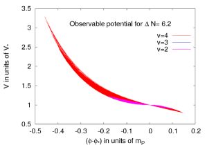
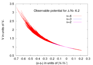
Figure 2: Left: The shape of the scalar potential at the $95\%$-confidence level, normalized to the value of the potentials at the pivot scale. Right: The same, in a normalization such that all first derivatives are equal, and focus can be laid on the higher derivatives.

Finally, in Figure 2 the inflaton potential as bounded by present observations up to $95\%$ confidence level is shown, allowing up to second, third and fourth derivative.

4 Discussion

Previous works relied on an extrapolation of data over a range which is an order of magnitude broader than the range of the data itself, which is fine from one point of view. Focusing on the data only, these are the first results to constrain to potential up to such a high order.

In equations (1,2), one sees that $V(\phi)$ does not unambiguously define $H(\phi)$, however any $H(\phi)$ would uniquely define $V(\phi)$. Hence the defining quantity should be $H(\phi)$, which will be subject to a future work [12].

References

- [1] A. A. Starobinsky. Phys. Lett., B91:99–102, 1980; A. H. Guth. Phys. Rev., D23:347–356, 1981; K. Sato. Mon. Not. Roy. Astron. Soc., 195:467–479, 1981; S. W. Hawking and I. G. Moss. Phys. Lett., B110:35, 1982; A. D. Linde. Phys. Lett., B108:389–393, 1982; A. D. Linde. Phys. Lett., B129:177–181, 1983.
- [2] A. A. Starobinsky. JETP Lett., 30:682–685, 1979; S. W. Hawking. Phys. Lett., B115:295, 1982; A. A. Starobinsky. Phys. Lett., B117:175–178, 1982; A. H. Guth and S. Y. Pi. Phys. Rev. Lett., 49:1110–1113, 1982; A. D. Linde. Phys. Lett., B116:335, 1982; J. M. Bardeen, P. J. Steinhardt, and M. S. Turner. Phys. Rev., D28:679, 1983; L. F. Abbott and M. B. Wise. Nucl. Phys., B244:541–548, 1984; D. S. Salopek, J. R. Bond, and J. M. Bardeen. Phys. Rev., D40:1753, 1989.
- [3] P. J. Steinhardt and M. S. Turner. Phys. Rev., D29:2162–2171, 1984; D. S. Salopek and J. R. Bond. Phys. Rev., D42:3936–3962, 1990; A. R. Liddle, P. Parsons, and J. D. Barrow. Phys. Rev., D50:7222–7232, [astro-ph/9408015], 1994. S. M. Leach,A. R. Liddle, J. Martin and D. J. Schwarz. Phys. Rev., D66:023515, [astro-ph/0202094], 2002.
- [4] D. N. Spergel et al. Astrophys. J. Suppl., 170:377, [astro-ph/0603449], 2007.
- [5] H. Peiris and R. Easther. JCAP, 0607:002, [astro-ph/0603587], 2006; H. J. de Vega and N. G. Sanchez. astro-ph/0604136, 2006; W. H. Kinney, E. W. Kolb, A. Melchiorri, and A. Riotto. Phys. Rev., D74:023502, [astro-ph/0605338], 2006; J. Martin and C. Ringeval. JCAP, 0608:009, [astro-ph/0605367], 2006; L. Covi, J. Hamann, A. Melchiorri, A. Slosar, and I. Sorbera. Phys. Rev., D74:083509, [astro-ph/0606452], 2006; F. Finelli, M. Rianna, and N. Mandolesi. JCAP, 0612:006, [astro-ph/0608277], 2006; H. Peiris and R. Easther. JCAP, 0610:017, [astro-ph/0609003], 2006; C. Destri, H. J. de Vega, and N. G. Sanchez. [astro-ph/0703417], 2007; C. Ringeval. [astro-ph/0703486], 2007; A. Cardoso. Phys. Rev., D75:027302, [astro-ph/0610074], 2007;
- [6] R. Easther and H. Peiris. JCAP, 0609:010, [astro-ph/0604214], 2006;
- [7] J. Lesgourgues and W. Valkenburg. Phys. Rev., D75:123519, [astro-ph/0703625], 2007.
- [8] B. A. Powell and W. H. Kinney, JCAP 0708 (2007) 006 [arXiv:0706.1982 [astro-ph]].
- [9] L. Page et al. Astrophys. J. Suppl., 170:335, [astro-ph/0603450], 2007; G. Hinshaw et al. Astrophys. J. Suppl., 170:288, [astro-ph/0603451], 2007; N. Jarosik et al. Astrophys. J. Suppl., 170:263, [astro-ph/0603452], 2007.
- [10] M. Tegmark et al. Phys. Rev., D74:123507, [astro-ph/0608632], 2006.
- [11] A. Lewis and S. Bridle. Phys. Rev., D66:103511, [astro-ph/0205436], 2002.
- [12] A. A. Starobinsky, J. Lesgourgues and W. Valkenburg. work in progress.