Remerciements

Par cette première page, je dédicace ce manuscrit à toutes les personnes qui m’ont aidé et soutenu pendant ces trois dernières années.

Je remercie sincèrement Johann Collot et Serge Kox, directeurs du LPSC de Grenoble, de m’avoir accueilli au sein du laboratoire durant ma thèse.

Mes remerciements s’adressent également à mes rapporteurs, Aldo Deandrea et John Ellis, ainsi qu’aux membres de mon jury, Wolfgang Hollik, Serge Kox, François Le Diberder et Gérard Sajot, pour leur lecture attentive de ce manuscrit, leurs commentaires et suggestions.

Entamer une thèse consiste à débuter un long travail, et ce travail ne peut être effectué sans guide. J’aimerais remercier Michael, mon directeur de thèse, qui m’a accordé sa confiance tout au long de ces trois années. En février 2004, tu m’as proposé un sujet de thèse en physique théorique des particules alors que je n’avais jamais effectué le moindre travail de recherche dans ce domaine. Depuis, je pense m’être rattrapé, les projets s’étant succédés les uns aux autres. J’aimerais également te témoigner ma plus sincère reconnaissance pour la patience et la gentillesse dont tu as fait preuve face à mes innombrables questions, et pour nos discussions, sans quoi ce travail ne serait pas ce qu’il est aujourd’hui. J’espère de tout cœur que notre collaboration durera encore de nombreuses années. Encore merci.

Dès le début de ma thèse, le jeune novice que j’étais put bénéficier des conseils et de l’expérience d’un post-doc avisé, Giuseppe. J’ai essayé de t’apprendre quelques expressions du parler bruxellois. En échange, tu m’as enseigné que foncer tête baissée dans un tas de problèmes afin d’y extirper les solutions n’est pas toujours la méthode la plus efficace, et qu’il vaut parfois mieux prendre du recul et attaquer les problèmes un par un. De plus, m’avoir comme voisin de bureau n’a sans doute pas toujours été très facile, et je te remercie pour ta disponibilité et ton aide.

Un clin d’œil à Björn, qui me montra qu’il n’y avait pas que les collisionneurs dans la vie, mais également la cosmo. Parmi nos exploits, il faudra retenir que nous avons prouvé que l’homme est plus malin que Mathematica (ou pas). Fin septembre, je m’en irai vers de nouvelles contrées, mais la relève est très prometteuse. Bon courage pour ta thèse, Jonathan.

Bien sûr, je ne peux oublier l’équipe des physiciens de Grenoble. Sabine pour la relecture du manuscrit, Guillaume pour les suggestions concernant le résumé en français, Benoît, Bertrand, Ingo, Jean-Marc et Ji-Young pour avoir assisté aux répétitions de soutenance, et les membres du groupe de physique théorique, qui sont autant amateurs de pique-niques que de physique. Je tiens ensuite à remercier l’ensemble des habitants du royaume du Bidul, fervents adorateurs de la sacro-sainte pause-café de midi qui dure des heures. Par ordre alphabétique, Antje, Colas, Florent, Jonathan, Julien, Julien, Kevin, Lauranne, Marie-Anne, Maud, Pierre-Antoine, Stéphanie, Sylvain, Thibaud, Vincent, Yoann, et ceux déjà cités auparavant.

Parfois, les rouages de l’administration peuvent paraître simples, surtout avec Cécile et France pour vous aider à y voir plus clair. Merci à toutes les deux pour votre disponibilité et votre gentillesse.

Je désire également écrire une petite dédicace à Daniel Baye dont le cours d’éléments de mécanique quantique a hautement influencé mon choix concernant la voie de la physique.

Évidemment, je ne peux clore ces lignes sans une pensée pour mes proches, ma famille et mes amis. Une attention toute particulière pour mes parents, mes grands-parents, et mes frères qui me soutiennent et supportent depuis toujours, ainsi que pour Marraine Vera et Parrain John qui ont fait le déplacement jusqu’à Grenoble pour assister à ma soutenance. Ses encouragements, son soutien et sa bonne humeur n’ont jamais tenu compte des frontières; un grand merci à toi, Manou. Je remercie également mes amis, de Bruxelles, de Grenoble, ou d’ailleurs, et spécialement Catherine, Donio et Julien qui n’ont pas eu peur des kilomètres pour venir assister à ma présentation, ainsi qu’Aline, Benoît, Elise, Fab, Floh, Gima, Jean-Louis, Jonathan, Karo, Lolo, Mélanie, Myriam, Nico, Sophie, Wawaa et Yann pour leur soutien sans faille.

Pour ceux que j’aurais oubliés, je ne l’ai pas fait exprès, mais merci à vous.

Abstract

Cross sections for supersymmetric particles production at hadron colliders have been extensively studied in the past at leading order and also at next-to-leading order of perturbative QCD. The radiative corrections include large logarithms which have to be resummed to all orders in the strong coupling constant in order to get reliable perturbative results. In this work, we perform a first and extensive study of the resummation effects for supersymmetric particle pair production at hadron colliders. We focus on Drell-Yan like slepton-pair and slepton-sneutrino associated production in minimal supergravity and gauge-mediated supersymmetry-breaking scenarios, and present accurate transverse-momentum and invariant-mass distributions, as well as total cross sections.

In non-minimal supersymmetric models, novel effects of flavour violation may occur. In this case, the flavour structure in the squark sector cannot be directly deduced from the trilinear Yukawa couplings of the fermion and Higgs supermultiplets. We perform a precise numerical analysis of the experimentally allowed parameter space in the case of minimal supergravity scenarios with non-minimal flavour violation, looking for regions allowed by low-energy, electroweak precision, and cosmological data. Leading order cross sections for the production of squarks and gauginos at hadron colliders are implemented in a flexible computer program, allowing us to study in detail the dependence of these cross sections on flavour violation.

Les sections efficaces de production hadronique de particules supersymétriques ont été largement étudiées par le passé, aussi bien à l’ordre dominant qu’à l’ordre sous-dominant en QCD perturbative. Les corrections radiatives incluent de larges termes logarithmiques qu’il faut resommer à tous les ordres afin d’obtenir des prédictions consistantes. Dans ce travail, nous effectuons une première étude détaillée des effets de resommation pour la production hadronique de particules supersymétriques. Nous nous concentrons sur la production de type Drell-Yan de sleptons et sur la production associée d’un slepton et d’un sneutrino dans des scénarios de supergravité minimale et de brisure de supersymétrie véhiculée par interactions de jauge, et nous présentons des distributions d’impulsion transverse et de masse invariante, ainsi que des sections efficaces totales.

Dans les modèles supersymétriques non minimaux, de nouveaux effets de violation de la saveur peuvent avoir lieu. Dans ce cas, la structure de saveur dans le secteur des squarks ne peut pas être déduite directement du couplage trilinéaire entre les supermultiplets de Higgs et de fermions. Nous effectuons une analyse numérique de l’espace des paramètres permis dans le cas de scénarios de supergravité minimale avec violation de la saveur non minimale, cherchant les régions permises par les mesures de précision électrofaibles, les observables à basse énergie et les données cosmologiques. La dépendance des sections efficaces à l’ordre dominant pour la production hadronique de squarks et de jauginos par rapport à la violation de la saveur non minimale est étudiée en détails.

  

Contents

1. 1 Introduction
2. 2 The Minimal Supersymmetric Standard Model
   1. 2.1 Motivation
   2. 2.2 Definition of the model
      1. 2.2.1 Field content
      2. 2.2.2 Lagrangian density
      3. 2.2.3 Soft SUSY-breaking
      4. 2.2.4 Electroweak symmetry breaking and particle mixing
   3. 2.3 The MSSM with non-minimal flavour violation
      1. 2.3.1 The model
      2. 2.3.2 Experimental constraints on flavour violating SUSY
      3. 2.3.3 Scan of the mSUGRA parameter space
      4. 2.3.4 NMFV benchmark points and slopes
   4. 2.4 Generalized couplings
3. 3 Resummation formalisms
   1. 3.1 General points
      1. 3.1.1 Main features of the resummation procedure
      2. 3.1.2 Soft-photon resummation in QED
      3. 3.1.3 Soft-gluon resummation in QCD
   2. 3.2 Transverse-momentum resummation
      1. 3.2.1 The Collins-Soper-Sterman (CSS) formalism
      2. 3.2.2 Non-perturbative effects in the CSS formalism
      3. 3.2.3 Disadvantages of the CSS formalism
      4. 3.2.4 Universal resummation formalism
      5. 3.2.5 Inverse transforms and matching procedure
   3. 3.3 Threshold resummation
      1. 3.3.1 Formalism
      2. 3.3.2 Improvements of the resummation formalism
      3. 3.3.3 Inverse Mellin transform and matching procedure
   4. 3.4 Joint resummation
      1. 3.4.1 Formalism
      2. 3.4.2 Reorganization of the resummed cross section
      3. 3.4.3 Inverse transform and matching
   5. 3.5 Comparison between $q_{T}$, threshold and joint resummations
4. 4 Slepton-pair production at hadron colliders
   1. 4.1 LO unpolarized cross section and spin asymmetries
      1. 4.1.1 Analytical results
      2. 4.1.2 Unpolarized cross section
      3. 4.1.3 Single-spin asymmetries
   2. 4.2 Transverse-momentum spectrum
      1. 4.2.1 Analytical results
      2. 4.2.2 Numerical results
   3. 4.3 Invariant-mass distributions
      1. 4.3.1 Next-to-leading order calculations
      2. 4.3.2 Threshold-enhanced contributions
      3. 4.3.3 Numerical results
   4. 4.4 Total cross section at NLO
   5. 4.5 Jointly resummed results
5. 5 Squark and gaugino production and decays at hadron colliders
   1. 5.1 NMFV squark-antisquark pair hadroproduction
      1. 5.1.1 Analytical results
      2. 5.1.2 Numerical results
      3. 5.1.3 cMFV limit
      4. 5.1.4 QCD one-loop contributions for non-diagonal squark pair production
      5. 5.1.5 Double-spin asymmetries
   2. 5.2 NMFV squark pair production
      1. 5.2.1 Analytical results
      2. 5.2.2 Numerical results
   3. 5.3 NMFV associated production of squarks and gauginos
      1. 5.3.1 Analytical results
      2. 5.3.2 Numerical results
   4. 5.4 NMFV gaugino pair production
      1. 5.4.1 Analytical results
      2. 5.4.2 Numerical results
   5. 5.5 Impact of flavour violation on squark and gaugino production
   6. 5.6 NMFV decays of squarks, gluino and gauginos
      1. 5.6.1 Squark decays
      2. 5.6.2 Gluino decays
      3. 5.6.3 Gaugino decays
6. 6 Conclusion and outlook

Résumé

Le Modèle Standard (SM) de la physique des particules [1, 2, 3, 4, 5, 6, 7] décrit avec succès un grand nombre de données expérimentales de haute énergie. Cependant, certaines questions fondamentales restent sans réponse, comme par exemple les origines de la brisure de la symétrie électrofaible et des masses des particules, la large hiérarchie entre l’échelle de Planck et l’échelle électrofaible, le mécanisme responsable des oscillations de neutrinos, les origines de la matière sombre et de la constante cosmologique, ou encore le problème CP lié à l’interaction forte. Les tentatives visant à relier différents paramètres du SM mènent en général à des théories plus fondamentales qui résolvent naturellement certains de ces problèmes ouverts.

La philosophie générale des Théories de Grande Unification (GUTs) [8, 9, 10] est de considérer que les groupes de symétrie du SM émergent de la brisure d’un groupe simple de rang plus élevé. A l’échelle GUT, les trois constantes de couplage de jauge du SM sont unifiées, et les quarks et les leptons sont décrits par des représentations communes de ce groupe de jauge plus large. Ces théories prédisent en général un certain nombre de bosons de jauge additionnels, menant éventuellement à des interactions pouvant violer la conservation des nombres baryonique et leptonique. Il s’agit de l’un des problèmes phénoménologiques les plus importants pour les GUTs, vu que les baryons sont alors instables, ce qui est contraire aux données expérimentales liées à la non observation de la désintégration du proton. Les théories GUTs peuvent expliquer la quantification de la charge électrique et incorporer des neutrinos massifs, mais ont quelques difficultés pour reproduire la valeur mesurée de l’angle de mélange électrofaible. De plus, un grand nombre de problèmes conceptuels déjà présents dans le SM demeurent sans réponse.

Une approche populaire pour résoudre le problème de hiérarchie du SM est d’ajouter à l’espace-temps des dimensions supplémentaires [11, 12]. Dans ce cadre théorique, les interactions de jauge et gravitationnelle sont unies à une échelle proche de l’échelle électrofaible, qui est alors la seule échelle fondamentale de la théorie, la valeur importante de l’échelle de Planck étant seulement une conséquence de la présence des nouvelles dimensions. L’espace à quatre dimensions habituel est contenu dans une “brane” quadridimensionnelle, elle-même incluse dans une structure plus large contenant N dimensions additionnelles, le “bulk”. Dans ces théories, chaque champ du SM possède une série d’excitations de Kaluza-Klein avec les mêmes nombres quantiques, mais une masse différente. Au jour d’aujourd’hui, ces excitations n’ont pas encore été observées, mais l’ordre de grandeur de leur masse est le TeV, ce qui les rend tout à fait détectables au futur Grand Collisionneur de Hadrons, le LHC, au CERN.

Plus récemment, d’autres tentatives pour résoudre ce problème de hiérarchie ont été proposées, comme par exemple les théories “Little-Higgs” ou “Twin-Higgs”, qui prédisent également de nouvelles particules avec des masses de l’ordre du TeV [13, 14, 15]. Ces théories incluent des partenaires fermioniques pour les quarks et les leptons du SM, et des partenaires bosoniques pour les bosons de jauge. Cela permet la stabilisation de la masse du boson de Higgs au-delà de l’ordre dominant grâce à la réalisation d’une symétrie non linéaire reliant les couplages au boson de Higgs d’une façon telle que les divergences venant des corrections quantiques s’annulent.

Dans cette thèse, nous nous concentrons sur une autre extension attractive du SM, la supersymétrie (SUSY) [16, 17, 18, 19, 20], et plus précisément le Modèle Standard Supersymétrique Minimal (MSSM) [21, 22]. La supersymétrie à basse énergie fournit une solution naturelle à plusieurs des problèmes conceptuels du SM. Reliant les fermions et les bosons, elle permet la stabilisation de la hiérarchie séparant l’échelle de Planck de l’échelle électrofaible [23, 24] et l’unification des couplages de jauge aux hautes énergies [25, 26, 27, 28]. De plus, la particule SUSY la plus légère peut dans certains cas être vue comme un candidat potentiel pour la matière sombre [29, 30]. Vu que les partenaires supersymétriques des particules du SM n’ont pas encore été observés jusqu’à présent, la supersymétrie doit être brisée à basse énergie, mais de façon douce afin qu’elle reste une solution viable pour le problème de la hiérarchie. Les particules SUSY sont donc plus massives que leurs équivalents du SM, mais leur masse ne devrait pas excéder quelques TeV. Une recherche concluante couvrant un large régime de masses allant jusqu’à l’échelle du TeV est donc l’un des points principaux du programme expérimental des collisionneurs hadroniques présents et futurs, comme par exemple le Tevatron à Fermilab ou le LHC au CERN.

Les sections efficaces de production des particules SUSY auprès des collisionneurs hadroniques ont été étudiées en détail par le passé, aussi bien à l’ordre dominant (LO) [31, 32, 33] qu’à l’ordre sous-dominant (NLO) [34, 35, 36, 37, 38, 39, 40] en QCD perturbative. Il est connu que les corrections NLO QCD [39] et NLO SUSY-QCD complètes [40] pour la production d’une paire de sleptons augmentent les sections efficaces hadroniques d’environ 35% au Tevatron et 25% au LHC, ce qui étend le potentiel de découverte des sleptons de plusieurs dizaines de GeV. Cependant, les corrections SUSY sont bien plus faibles que leurs analogues QCD en raison de la présence de squarks et gluinos très lourds dans les boucles.

Malgré le succès des premières collisions proton-proton en mode polarisé au collisionneur RHIC, les sections efficaces polarisées ont reçu bien moins d’attention que leurs équivalents non polarisés. Les calculs pionniers pour la production de squarks et de gluinos non massifs [41, 42] n’ont été vérifiés, généralisés au cas de particules SUSY massives et appliqués aux collisionneurs actuels que récemment [43]. Concernant la production de sleptons, seulement des calculs négligeant les mélanges entre les états propres d’hélicité étaient disponibles, et appliqués uniquement à des expériences d’anciens collisionneurs [44].

En raison de leurs couplages purement électrofaibles, les sleptons sont parmi les particules SUSY les plus légères dans de nombreux scénarios de brisure de supersymétrie [45, 46]. Les sleptons et sneutrinos se désintègrent souvent directement en la particule SUSY la plus légère (le neutralino le plus léger dans les modèles de supergravité minimale (mSUGRA) ou le gravitino pour la brisure de supersymétrie véhiculée par interactions de jauge (GMSB)) et le partenaire du SM correspondant (un lepton ou un neutrino). Ainsi, un signal relatif à une paire de sleptons produite en collisionneur hadronique consistera en une paire de leptons très énergétiques, qui sera facilement détectable, et de l’énergie manquante associée.

Dans cette thèse, nous avons vérifié les calculs pionniers pour la production polarisée d’une paire de sleptons [44], que nous avons ensuite généralisés afin de prendre en compte le mélange des états propres d’interaction, qui est surtout pertinent pour les sleptons de troisième génération. Nous présentons les résultats analytiques pour les courants de sleptons neutres et chargés, et prédisons numériquement les asymétries simple-spin pour le collisionneur RHIC et pour d’éventuelles améliorations du Tevatron et du LHC où l’un des faisceaux est polarisé. Nous avons mis en évidence la sensibilité de l’asymétrie simple-spin à l’angle de mélange du slepton tau et la possibilité de l’utiliser comme moyen pour distinguer le signal SUSY du bruit de fond du SM correspondant à la production Drell-Yan d’une paire de leptons [47].

Le bruit de fond standard principal lié à la production hadronique d’une paire de sleptons vient des désintégrations de paires $WW$ et $t\bar{t}$ en une paire de leptons et de l’énergie manquante [48, 49]. Deux éléments clés pour distinguer le signal SUSY du bruit de fond standard sont la reconstruction de la masse et la détermination du spin des particules produites. Pour une paire de sleptons, la masse (s)transverse de Cambridge est une observable particulièrement utile, puisqu’une connaissance précise du spectre en impulsion transverse ($q_{T}$) suffit alors pour déterminer la masse [50] et le spin [51] des sleptons.

Lorsque que l’on étudie la distribution en impulsion transverse d’un système non coloré produit avec une masse invariante $M$ lors d’une collision hadronique, il est pertinent de séparer les régions cinématiques relatives aux larges et aux faibles valeurs de $q_{T}$. Dans la région des $q_{T}$ importants ($q_{T}\geq M$), l’utilisation de la théorie perturbative à ordre fixé est parfaitement justifiée, vu que le développement en série de la distribution en $q_{T}$ est contrôlé par un paramètre d’expansion de faible valeur, la constante de couplage forte $\alpha_{s}(M^{2})$. Dans la région des petites valeurs de $q_{T}$, les coefficients du développement perturbatif sont amplifiés par des termes logarithmiques importants, $\ln(M^{2}/q_{T}^{2})$, et les résultats basés sur des calculs perturbatifs divergent pour $q_{T}\to 0$, la convergence de la série étant alors complètement détruite. Ces logarithmes proviennent de l’émission multiple de gluons mous par l’état initial, et doivent être systématiquement resommés à tous les ordres en $\alpha_{s}$ afin d’obtenir des résultats consistants. La méthode pour effectuer cette resommation est bien connue [52, 53, 54, 55, 56, 57, 58, 59, 60, 61, 62]. La resommation des logarithmes dominants a été effectuée pour la première fois en [52]. Il a été montré en [53] que la procédure de resommation est plus naturellement effectuée dans l’espace du paramètre d’impact $b$, $b$ étant la variable conjuguée à $q_{T}$ via une transformation de Fourier. En effet, dans ce cas-là, la cinématique de l’émission multiple de gluons factorise complètement. Dans les cas particuliers de la production Drell-Yan d’une paire de leptons et de la production d’un boson électrofaible, la resommation dans l’espace $b$ a été effectuée au niveau sous-dominant (NLL) [55], un formalisme de resommation consistant à n’importe quelle précision logarithmique a été développé [59], et les termes d’ordre sous-sous-dominant ont été calculés [60]. Pour les valeurs de $q_{T}$ intermédiaires, le résultat resommé doit être ajusté de façon consistante avec celui basé sur la théorie perturbative, afin d’obtenir des prédictions d’une précision théorique uniforme sur tout le domaine d’impulsion transverse considéré.

Dans ce travail, nous avons implémenté le formalisme de resommation en $q_{T}$ proposé en [61, 62], et prédit le spectre en impulsion transverse pour la production d’une paire de sleptons au LHC. Nous avons combiné le résultat resommé (valide pour les faibles valeurs de $q_{T}$), calculé au niveau NLL, avec la section efficace à ordre fixé (valide pour les larges valeurs de $q_{T}$), calculée à l’$\mathcal{O}(\alpha_{s})$ en QCD perturbative qui correspond à la production d’une paire de sleptons associée à un jet QCD [63]. Il s’agit du premier calcul de précision concernant la distribution en impulsion transverse pour un processus de production d’une paire de particules SUSY auprès d’un collisionneur hadronique. Dans nos résultats numériques, nous avons montré l’importance de la resommation aussi bien pour les faibles valeurs de $q_{T}$ que pour les valeurs intermédiaires. Par ailleurs, la resommation permet de réduire la dépendance de la distribution en $q_{T}$ en les échelles non physiques de factorisation et de renormalisation. Nous avons également étudié l’influence des contributions non perturbatives sur le résultat resommé, et observé qu’elle était réduite par rapport à l’effet de la resommation.

En ce qui concerne les corrections NLO SUSY-QCD, elles ont été calculées uniquement en négligeant le mélange des états propres d’interaction des squarks apparaissant dans les boucles [40]. Nous avons généralisé ce travail en incluant ce mélange pertinent pour les squarks de troisième génération, et avons considéré les effets de seuil provenant de l’émission de gluons mous par l’état initial. Lorsque les partons initiaux ont tout juste assez d’énergie pour produire la paire de sleptons dans l’état final, les corrections virtuelles et l’émission de gluons réels supprimée par l’espace de phase mènent à l’apparition de termes logarithmiques importants $\alpha_{s}^{n}[\ln^{2n-1}(1-z)/(1-z)]_{+}$ à l’ordre $n$ de la théorie perturbative, où $z=M^{2}/s$, $s$ est l’énergie dans le centre de masse partonique et $M$ la masse invariante de la paire de sleptons. Lorsque $s$ est proche de $M^{2}$, ces logarithmes doivent être resommés à tous les ordres en $\alpha_{s}$. Bien que ces divergences apparaissent de façon explicite dans la section efficace partonique, la section efficace hadronique n’est en général pas divergente en raison de la convolution avec les densités de partons très faibles pour les grandes valeurs de la fraction d’impulsion longitudinale du proton correspondant aux valeurs de $z$ proches de un. La resommation en seuil est donc plutôt une tentative de quantification de l’effet d’un ensemble de corrections bien définies qu’une simple somme de logarithmes d’origine cinématique. Ces effets peuvent cependant être significatifs même loin du seuil hadronique, et l’on s’attend donc à des corrections importantes pour la section efficace de production de type Drell-Yan d’une paire de sleptons de quelques centaines de GeV au Tevatron et au LHC.

La resommation en seuil à tous les ordres en $\alpha_{s}$ équivaut à l’exponentiation des radiations de gluons mous, et n’a pas lieu dans l’espace $z$ directement, mais dans l’espace $N$ de Mellin, où $N$ est la variable conjuguée à $z$ par une transformation de Mellin, la région du seuil $z\to 1$ correspondant à la limite $N\to\infty$. Ainsi, la section efficace resommée dans l’espace $z$ sera obtenue après une transformation inverse finale. La resommation en seuil pour le processus Drell-Yan fut d’abord effectuée en [64, 65] aux niveaux logarithmiques dominant et sous-dominant (NLL), correspondant à la resommation des termes de type $\alpha_{s}^{n}\ln^{2n}N$ et $\alpha_{s}^{n}\ln^{2n-1}N$. L’extension au niveau NNLL (termes de type $\alpha_{s}^{n}\ln^{2n-2}N$) a également été effectuée à la fois pour le processus Drell-Yan [66] et pour la production d’un boson de Higgs [67]. Il a été montré [68, 69] que les contributions dues à l’émission de partons colinéaires peuvent également être incluses de façon consistante dans la formule de resommation. Cela correspond au formalisme de resommation “amélioré colinéairement”, où des termes contenant un facteur suppressif $1/N$ et une classe de contributions universelles indépendantes de $N$ sont également resommés. Très récemment, les contributions à l’ordre NNNLL (les termes de type $\alpha_{s}^{n}\ln^{2n-3}N$) ont été calculées [70, 71, 72].

Nous présentons ici une étude détaillée des effets de la resommation en seuil pour la production de type Drell-Yan d’une paire de sleptons et pour la production associée d’un slepton et d’un sneutrino dans le cadre de scénarios mSUGRA et GMSB. Nous avons ajusté les résultats resommés à la précision NLL, calculés grâce au formalisme de resommation amélioré colinéairement, avec les résultats basés sur la théorie perturbative calculés à la précision NLO. Numériquement, nous avons montré une augmentation non négligeable de la section efficace théorique par rapport aux prédictions NLO, et une stabilisation de la dépendance en les échelles non physiques grâce à l’apport des termes d’ordres supérieurs pris en compte par la resommation [73].

L’origine dynamique des contributions logarithmiques intervenant dans les formalismes de resommation en impulsion transverse et en seuil est identique, vu qu’il s’agit de l’émission multiple de gluons mous par l’état initial. Un formalisme de resommation jointe, prenant en compte simultanément les contributions des gluons mous dans les deux régions cinématiques concernées ($q_{T}\ll M$ et $M^{2}\sim s$) a été développé dans la dernière décade [74, 75]. L’exponentiation des termes singuliers dans les espaces de Mellin et du paramètre d’impact, pour la resommation en seuil et en impulsion transverse respectivement, a été prouvée, et une méthode consistante pour effectuer les transformations inverses a été introduite afin d’éviter le pôle de Landau et les singularités dues aux densités de partons. Les applications de ce formalisme à la production hadronique d’un photon rapide [76], d’un boson électrofaible [77], d’un boson de Higgs [78], et d’une paire de quarks lourds [79] montrent les effets de la resommation sur différentes distributions.

Nous présentons dans ce travail un traitement joint des corrections à faible impulsion transverse et des contributions importantes proche du seuil partonique pour la production d’une paire de sleptons auprès des collisionneurs hadroniques, ce qui permet une compréhension complète des effets de gluons mous pour le spectre en impulsion transverse et pour les distributions en masse invariante. Avec le travail sur la resommation en impulsion transverse [63] et la resommation en seuil [73], cette étude [80] complète notre programme ayant pour but de fournir les premiers calculs de précision incluant la resommation de gluons mous pour la production de sleptons auprès des collisionneurs hadroniques.

Si les particules SUSY existent, elles doivent aussi apparaître dans les boucles de particules virtuelles et affecter les observables de précision électrofaibles et les observables à basse énergie. Plus particulièrement, les courants neutres à changement de saveur qui apparaissent seulement au niveau des boucles dans le SM contraignent sévèrement les contributions de nouvelle physique au même ordre perturbatif. Le MSSM se libère de ces contraintes grâce aux hypothèses de Violation de Saveur Minimale contrainte (cMFV) [81, 82] ou de Violation de Saveur Minimale (MFV) [83, 84, 85], où les particules SUSY peuvent intervenir dans les boucles, mais les changements de saveur sont soit négligés, soit complètement dictés par la structure des couplages de Yukawa et par la matrice CKM [86, 87].

En SUSY avec MFV, les éléments des matrices de masse des squarks violant la saveur découlent des couplages trilinéaires de Yukawa entre les supermultiplets de Higgs et de fermions et des différentes renormalisations des secteurs des quarks et des squarks via les équations du groupe de renormalisation qui induisent des violations de saveur supplémentaires à l’échelle électrofaible [88, 89, 90, 91]. En SUSY avec violation de saveur non minimale, des sources de violation de saveur additionnelles sont incluses dans les matrices de masse et leurs termes non diagonaux qui ne peuvent plus être simplement déduits à partir de la matrice CKM seule doivent être considérés alors comme des paramètres libres. Dans ce travail, nous allons considérer le mélange des saveurs de squark de deuxième et troisième générations, car d’une part, les recherches directes de violation de la saveur dépendent des capacités à déterminer la saveur, ce qui n’est expérimentalement bien établi que pour les saveurs lourdes, et d’autre part, des contraintes expérimentales sévères pour la première génération existent en raison de mesures très précises des oscillations $K^{0}-\bar{K}^{0}$ et des premières preuves du mélange $D^{0}-\bar{D}^{0}$ [92, 93, 94].

Nous avons analysé l’espace des paramètres NMFV SUSY, recherchant les régions permises par les contraintes venant des mesures de précision électrofaibles, des observables à basse énergie et des données cosmologiques. Nous avons observé que le mélange des chiralités et des saveurs de deuxième et troisième générations est fortement contraint, notamment par l’erreur expérimentale de plus en plus petite sur le rapport d’embranchement $b\to s\gamma$ et la densité relique de matière sombre. Nous avons défini quatre nouveaux points typiques avec leur ligne associée, valides à la fois en SUSY avec cMFV, MFV et NMFV, et pour lesquels nous présentons la dépendance des masses de squarks et de la décomposition des états physiques de squark en la violation de la saveur.

Considérant la SUSY avec cMFV (le MSSM habituel), les corrections SUSY-QCD pour la production de squarks et de gluinos [34], de jauginos [40], ainsi que pour leur production associée [37] ont déjà été calculées. En raison de leur couplage fort, les squarks devraient être produits abondamment aux collisionneurs hadroniques, et l’espace de phase favorise la production des états propres de masse les plus légers. Ainsi, les productions des squarks top [35] et bottom [95] avec un grand mélange d’hélicité ont reçu une attention toute particulière. Dans cette thèse, nous nous sommes intéressés à l’importance des canaux électrofaibles pour la production de paires de squarks non diagonales et mixtes de troisième génération aux collisionneurs hadroniques [96]. Naïvement, l’on s’attend à ce que ces sections efficaces, qui sont d’ordre deux en la constante de structure fine, $\mathcal{O}(\alpha^{2})$, soient plus faibles que celles concernant la production forte d’une paire de squarks diagonale d’environ deux ordres de grandeurs. Pour la production non diagonale, l’importance des canaux QCD est réduite en raison de la présence de boucles, et celle des canaux électrofaibles l’est également en raison du couplage faible. L’importance relative de ces canaux mérite donc une étude approfondie. Si l’on considère des squarks bottom qui se mélangent, leur contribution au niveau des boucles QCD doit également être prise en compte.

Ensuite, pour la première fois, nous nous sommes concentrés sur les effets possibles de la violation de saveur non minimale (NMFV) aux collisionneurs hadroniques [97]. A cette fin, nous avons recalculé toutes les amplitudes d’hélicité pour la production et la désintégration des squarks et des jauginos, en prenant en compte les interactions non diagonales des courants chargés des jauginos et les interactions de Yukawa des Higgsinos, et en généralisant les matrices de mélange d’hélicités bidimensionnelles, souvent supposées réelles, en matrices de mélange d’hélicités et de saveurs, complexes et six-dimensionnelles. Nous avons vérifié que nos résultats reproduisaient ceux de la littérature existant dans les limites de squarks non mélangés.

Dans notre analyse phénoménologique de la production NMFV de squarks et de jauginos, nous nous sommes concentrés sur le LHC en raison de son énergie dans le centre de masse élevée et de sa luminosité importante. Nous avons porté une attention particulière à la compétition entre les effets liés aux densités de partons qui sont dominés par les contributions des quarks légers, les contributions fortes du gluino qui sont généralement plus importantes que les contributions électrofaibles et qui ne doivent pas nécessairement être diagonales en saveur, et la présence de saveurs lourdes dans l’état final, facilement identifiables expérimentalement et généralement plus légères que les saveurs de squark de première et deuxième générations.

  

Chapter 1 Introduction

The Standard Model (SM) of particle physics [1, 2, 3, 4, 5, 6, 7] provides a successful description of all experimental high energy data. However, despite of its success many fundamental questions remain unanswered, e.g.  the origins of electroweak symmetry breaking and particle masses, the large hierarchy between the electroweak and the Planck scales, the mechanism leading to neutrino oscillations, the origins of dark matter and of the cosmological constant, or the strong CP-problem. Attempts to relate different SM parameters lead to more fundamental theories, that may at the same time solve some of the open problems of the SM.

The basic philosophy of Grand Unified Theories (GUTs) [8, 9, 10] is to consider the SM symmetry groups as originating from the breaking of a larger simple group. At the GUT scale, the three SM gauge coupling constants unify and quarks and leptons are embedded in common representations of the unifying gauge group. These theories include then number of additional gauge bosons, leading potentially to interactions violating the baryon and lepton numbers. This leads to one of the major phenomenological problems of GUTs, which predict baryon instability, contrary to the experimental non-observation of proton decay. GUT theories can explain the quantization of the electric charge and incorporate massive neutrinos, but have difficulties in accounting for the measured value of the electroweak mixing angle. Besides, many other conceptual SM problems remain unsolved.

One popular approach to solve the hierarchy problem of the SM is to extend space-time to higher dimensions [11, 12]. In this framework, the gravitational and gauge interactions become unified close to the weak scale, which is then the only fundamental scale of the theory. The large value of the Planck scale is only a consequence of the new dimensions. The usual four-dimensional space is contained in a four-dimensional “brane”, embedded in a larger structure with $N$ additional dimensions, the “bulk”. In these theories, each field of the SM possesses a tower of Kaluza-Klein excitations with the same quantum numbers, but different mass, which have not been observed at the present time, but which should lie in the TeV-range. They could then be detected at the future Large Hadron Collider (LHC) at CERN.

Recently, other attempts to solve the hierarchy problem have been proposed, e.g. Little-Higgs or Twin-Higgs theories, which predict new particles with masses in the TeV-range as well [13, 14, 15]. These theories include fermionic partners for quarks and leptons and bosonic partners for the SM gauge bosons, which allows for stabilization of the Higgs mass beyond tree-level thanks to a non-linearly realized symmetry that relates the couplings to the Higgs in such a way that the quantum corrections to the Higgs mass cancel.

In this thesis, we focus on another attractive extension of the SM, supersymmetry (SUSY) [16, 17, 18, 19, 20], and more precisely the Minimal Supersymmetric Standard Model (MSSM) [21, 22]. Weak scale supersymmetry provides a natural solution for a set of conceptual problems of the SM. Linking fermions with bosons, SUSY allows for a stabilization of the gap between the Planck scale and the electroweak scale [23, 24] and for a consistent unification of SM gauge couplings at high energies [25, 26, 27, 28]. In addition, it can include a potential dark matter candidate as the stable lightest SUSY particle [29, 30]. Since spin partners of the SM particles have not yet been observed and in order to remain a viable solution to the hierarchy problem, SUSY must be broken at low energy via soft mass terms in the Lagrangian. As a consequence, the SUSY particles must be massive in comparison to their SM counterparts, but their mass should not exceed a few TeV. A conclusive search covering a wide range of masses up to the TeV scale is then one of the main topics in the experimental program at present and future hadron colliders, such as the Tevatron at Fermilab and the LHC at CERN.

Production cross sections for SUSY particles at hadron colliders have been extensively studied in the past at leading order (LO) [31, 32, 33] and also at next-to-leading order (NLO) of perturbative QCD [34, 35, 36, 37, 38, 39, 40]. The NLO QCD [39] and full SUSY-QCD [40] corrections for slepton pair production are known to increase the hadronic cross sections by about 35 % at the Tevatron and 25% at the LHC, extending thus the discovery reaches of sleptons by several tens of GeV. However, the presence of massive squarks and gluinos in the loops makes the genuine SUSY corrections considerably smaller than the standard QCD ones.

Despite of the first successful runs of the RHIC collider in the polarized $pp$ mode, polarized cross sections have received much less attention. Only the pioneering LO calculations for massless squark and gluino production [41, 42] have recently been confirmed, extended to the massive case, and applied to current hadron colliders [43]. Concerning slepton pair production, only polarized calculations for non mixing sleptons were available before, and for old collider experiments only [44] .

Due to their purely electroweak couplings, sleptons are among the lightest SUSY particles in many SUSY-breaking scenarios [45, 46]. Sleptons and sneutrinos often decay directly into the stable lightest SUSY particle (the lightest neutralino in minimal supergravity (mSUGRA) models or the gravitino in gauge-mediated SUSY-breaking models (GMSB)) plus the corresponding SM partner (lepton or neutrino). As a result, a slepton signal at hadron colliders will consist in a highly energetic lepton pair, which will be easily detectable, and associated missing energy.

In this thesis, we verify the pioneering polarized calculations for slepton pair production [44] and extend them by including the mixing of the left- and right-handed interaction eigenstates relevant for third-generation sleptons. We present analytical results for neutral and charged current sleptons and make numerical predictions for longitudinal spin asymmetries at RHIC and possible upgrades of the Tevatron and the LHC, where one of the beams is considered to be polarized. We put particular emphasis on the sensitivity of the asymmetry to the tau slepton mixing angle as predicted by various SUSY-breaking mechanisms. Possibilities of using asymmetries to discriminate between the SUSY signal and the corresponding SM Drell-Yan background are also discussed [47].

The main SM background to slepton pair production at hadron colliders is due to $WW$ and $t\bar{t}$ decays to a lepton pair and missing energy [48, 49]. Two key features distinguishing the SUSY signal from the SM background are the reconstruction of the mass and the determination of the spin of the produced particles. For sleptons, the Cambridge (s)transverse mass proves to be a particularly useful observable, requiring only a precise knowledge of the transverse-momentum ($q_{T}$) spectrum to get their mass [50] and spin [51].

When studying the $q_{T}$-distribution of a colourless system produced with an invariant-mass $M$ in a hadronic collision, it is appropriate to separate the large-$q_{T}$ and small-$q_{T}$ regions. In the large-$q_{T}$ region ($q_{T}\geq M$) the use of fixed-order perturbation theory is fully justified, since the perturbative series is controlled by a small expansion parameter, the strong coupling constant $\alpha_{s}(M^{2})$. In the small-$q_{T}$ region, where the coefficients of the perturbative expansion in $\alpha_{s}(M^{2})$ are enhanced by powers of large logarithmic terms, $\ln(M^{2}/q_{T}^{2})$, results based on fixed-order calculations diverge as $q_{T}\to 0$, and the convergence of the perturbative series is spoiled. These logarithms are due to multiple soft-gluon emission from the initial state and have to be systematically resummed to all orders in $\alpha_{s}$ in order to obtain reliable perturbative predictions. The method to perform all-order soft-gluon resummation at small $q_{T}$ is well known [52, 53, 54, 55, 56, 57, 58, 59, 60, 61, 62]. The resummation of leading logarithms was first performed in [52]. It was shown in [53] that the resummation procedure is most naturally performed using the impact-parameter ($b$) formalism, where $b$ is the variable conjugate to $q_{T}$ through a Fourier transformation, to allow the kinematics of multiple-gluon emission to factorize. In the special case of Drell-Yan lepton pair or electroweak boson production, $b$-space resummation was performed at next-to-leading level in [55], a resummation formalism consistent at any logarithmic accuracy was developed in [59], and the next-to-next-to-leading order terms have been calculated in [60]. At intermediate $q_{T}$ the resummed result has to be consistently matched with fixed-order perturbation theory in order to obtain predictions with uniform theoretical accuracy over the entire range of transverse momenta.

We implement the universal $q_{T}$-resummation formalism proposed in [61, 62] and compute the $q_{T}$-distribution of a slepton pair produced at the LHC by combining resummation at small $q_{T}$ and the fixed-order cross section at large $q_{T}$. The resummed contribution has been computed at the next-to-leading logarithmic (NLL) accuracy and the fixed-order cross section at $\mathcal{O}(\alpha_{s})$ in perturbative QCD, corresponding to the production of a slepton pair plus a QCD jet. It is the first precision calculation of the $q_{T}$-spectrum for SUSY particle pair production at hadron colliders. The importance of resummed contributions at small and intermediate values of $q_{T}$, both enhancing the pure fixed-order result and reducing the scale uncertainty, is shown in our numerical results [63].

Concerning NLO SUSY-QCD corrections [40], they have only been computed for non-mixing squarks appearing in the loops. We extend this work by including the mixing effects relevant for the third generation in the squark sector, and we consider the threshold-enhanced contributions of the QCD corrections [39], also due to soft-gluon emission from the initial state. They arise when the initial partons have just enough energy to produce the slepton pair in the final state. In this case, the mismatch between virtual corrections and phase-space suppressed real-gluon emission leads to the appearance of large logarithmic terms $\alpha_{s}^{n}[\ln^{2n-1}(1-z)/(1-z)]_{+}$ at the $n^{{\rm th}}$ order of perturbation theory, where $z=M^{2}/s$, $s$ being the partonic centre-of-mass energy and $M$ the slepton pair invariant-mass. When $s$ is close to $M^{2}$, these large logarithms have to be resummed to all orders in $\alpha_{s}$. Although they are manifest in the partonic cross section, they do not generally result in divergences in the physical cross section since they are smoothed by the convolution with the steeply falling parton distributions. Threshold resummation is then not really a summation of kinematic logarithms in the physical cross section, but rather an attempt to quantify the effect of a well-defined set of corrections to all orders, which can be significant even if the hadronic threshold is far from being reached. Large corrections are thus expected for the Drell-Yan like production of a slepton pair with invariant-mass of a few 100 GeV at the Tevatron and LHC.

All-order resummation is achieved through the exponentiation of the soft-gluon radiation, which does not take place in $z$-space directly, but in Mellin $N$-space, where $N$ is the Mellin variable conjugate to $z$ and the threshold region $z\rightarrow 1$ corresponds to the limit $N\rightarrow\infty$. Thus, a final inverse Mellin transform is needed in order to obtain a resummed cross section in $z$-space. Threshold resummation for the Drell-Yan process was first performed in [64, 65] at the leading logarithmic and next-to-leading logarithmic (NLL) levels, corresponding to terms of the form $\alpha_{s}^{n}\ln^{2n}N$ and $\alpha_{s}^{n}\ln^{2n-1}N$. The extension to the NNLL level ($\alpha_{s}^{n}\ln^{2n-2}N$ terms) has been carried out both for the Drell-Yan process [66] and for Higgs-boson production [67]. It was shown in [68, 69] that contributions due to collinear parton emission can be consistently included in the resummation formula, leading to a “collinear-improved” resummation formalism where $1/N$-suppressed and a class of $N$-independent universal contributions are resummed as well. Very recently, even the NNNLL contributions ($\alpha_{s}^{n}\ln^{2n-3}N$ terms) became available [70, 71, 72].

We present here an extensive study on NLL threshold resummation effects for Drell-Yan like slepton pair and slepton-sneutrino associated production in mSUGRA and GMSB scenarios, matching the resummed contributions computed within a collinear-improved resummation formalism with a fixed-order calculation at NLO accuracy. Numerically, we show a non-negligible increase of the theoretical cross sections with respect to the NLO prediction and a stabilization of the unphysical scale dependences thanks to the higher order terms taken into account in the resummed component of the cross section [73].

The dynamical origin of the enhanced contributions is the same both in transverse-momentum and threshold resummations, since it comes from the soft-gluon emission by the initial state. A joint resummation formalism, embodying soft-gluon contributions in both the delicate kinematical regions ($q_{T}\ll M$, $M^{2}\sim s$) simultaneously, has been developed in the last decade [74, 75]. The exponentiation of the singular terms in the Mellin and impact-parameter spaces, for threshold and transverse-momentum resummation respectively, has been proven, and a consistent method to perform the inverse transforms in order to avoid the Landau pole and the singularities of the parton distribution functions has been introduced. Applications to prompt-photon [76], electroweak boson [77], Higgs boson [78] and heavy-quark pair [79] production at hadron colliders show the substantial effects of the joint resummation on the differential cross sections.

We present a joint treatment of the recoil corrections at small $q_{T}$ and the threshold-enhanced contributions near partonic threshold for slepton pair production at hadron colliders, allowing for a complete understanding of the soft-gluon effects in differential distributions [80]. Together with the previous papers on transverse-momentum [63] and threshold [73] resummation, this completes our program of providing the first precision calculations including soft-gluon resummation for slepton pair production at hadron colliders.

If SUSY particles exist, they should also appear in virtual particle loops and affect low-energy and electroweak precision observables. In particular, flavour-changing neutral currents (FCNC), which appear only at the one-loop level even in the SM, put severe constraints on new physics contributions appearing at the same perturbative order. The MSSM has passed these crucial tests, largely due to the assumption of constrained Minimal Flavour Violation (cMFV) [81, 82] or Minimal Flavour Violation (MFV) [83, 84, 85], where heavy SUSY particles may appear in the loops, but flavour changes are either neglected or completely dictated by the structure of the Yukawa couplings and thus the CKM-matrix [86, 87].

In SUSY with MFV, the flavour violating entries in the squark mass matrices stem from the trilinear Yukawa couplings of the fermion and Higgs supermultiplets and the resulting different renormalizations of the quark and squark mass matrices, which induce additional flavour violation at the weak scale through renormalization group running [88, 89, 90, 91]. In non-minimal flavour violating SUSY, additional sources of flavour violation are included in the mass matrices at the weak scale, and their flavour-violating off-diagonal terms cannot be simply deduced from the CKM matrix alone, and have to be considered as free parameters. In this work, we consider flavour mixings of second- and third-generation squarks, since direct searches of flavour violation depend on the possibility of flavour tagging, which is established experimentally only for heavy flavours. In addition, stringent experimental constraints for the first-generation are imposed by precise measurements of $K^{0}-\bar{K}^{0}$ mixing and first evidence of $D^{0}-\bar{D}^{0}$ mixing [92, 93, 94].

Considering SUSY with cMFV (the usual MSSM), NLO SUSY-QCD calculations for the production of squarks and gluinos [34], gauginos [40], as well as for their associated production [37] are available. Due to their strong coupling, squarks should be abundantly produced at hadron colliders. In addition, phase space favours the production of the lighter of the squark mass eigenstates of identical flavour. As a consequence, the production of top [35] and bottom [95] squarks with large helicity mixing has received particular attention. In this thesis, we investigate the importance of electroweak channels for non-diagonal and mixed squark pair production at hadron colliders [96]. Naively, one expects these cross sections, which are of ${\cal O}(\alpha^{2})$ in the fine structure constant $\alpha$, to be smaller than the diagonal strong channels by about two orders of magnitude. For non-diagonal squark production, the interplay between loop suppression in QCD and coupling suppression in the electroweak case merits a detailed investigation, and in the presence of the mixing of bottom squarks, their loop contributions must also be taken into account.

Then, for the first time, we concentrate on the possible effects of non-minimal flavour violation (NMFV) at hadron colliders [97]. To this end, we recalculate all squark and gaugino production and decay helicity amplitudes, keeping at the same time the CKM-matrix and the quark masses to account for non-diagonal charged-current gaugino and Higgsino Yukawa interactions, and generalizing the two-dimensional helicity mixing matrices, often assumed to be real, to generally complex six-dimensional helicity and generational mixing matrices.

In our phenomenological analysis of NMFV squark and gaugino production, we concentrate on the LHC due to its larger centre-of-mass energy and luminosity. We pay particular attention to the interesting interplay of parton density functions (PDFs), which are dominated by light quarks, strong gluino contributions, which are generally larger than electroweak contributions and need not be flavour-diagonal, and the appearance of third-generation squarks in the final state, which are easily identified experimentally and generally lighter than first- and second-generation squarks.

This thesis is organized as follows. In the first part of Chapt. 2, we briefly describe the MSSM within cMFV, showing several motivating arguments for SUSY and defining the model. In the second part of this chapter, we set up the notations that we use in the case of NMFV SUSY, and we perform a precise numerical analysis of the experimentally allowed NMFV SUSY parameter space with respect to low-energy constraints, leading to the definition of four collider-friendly benchmark points for which we investigate the corresponding helicity and flavour decomposition of the up- and down-type squarks. Finally, we introduce generalized couplings in order to compute compact analytical expression for the various cross sections calculated in this work. In Chapt. 3, we describe the two $q_{T}$-resummation formalisms (CSS and universal), the threshold-resummation formalism and the joint-resummation formalism that we have used in the case of slepton pair hadroproduction. Chapts. 4 and 5 are devoted to the results, the first one for slepton pair hadroproduction and the second one to squark and gaugino production and decays, and we show a large number of analytical and numerical results. Our conclusion and outlook are presented in Chapt. 6.

Chapter 2 The Minimal Supersymmetric Standard Model

2.1 Motivation

The Standard Model of particle physics is a gauge field theory based on the symmetry group $SU(3)\times SU(2)\times U(1)$, containing the electroweak [1, 2, 3, 4] and the strong [5, 6, 7] interactions and providing a remarkably accurate description of a large class of phenomena. It is well-established by the discovery of all its particle content, the Higgs boson excepted, and by precision measurements at colliders. However, a new framework will certainly be required, at least at the Planck scale $M_{P}=2.8\times 10^{18}$ GeV, where the quantum gravitational effects become important, but more probably at a lower scale, since the absence of new physics between the current experimental limit of several hundreds of GeV and $M_{P}$ is highly improbable. Moreover, this large gap leads to what is called the hierarchy problem [23, 24].

The origin of the masses in the SM is an isodoublet scalar Higgs field [98, 99, 100, 101, 102, 103], yielding electroweak symmetry breaking and one physical Higgs boson which couples to each SM fermion of mass $m_{f}$ with a strength driven by the Yukawa couplings $\lambda_{f}$. The quantum corrections $\Delta m_{H}^{2}$ to the Higgs squared mass $m_{H}^{2}$, where

$$m_{H}^{2}=(m_{H}^{2})_{0}+\Delta m_{H}^{2},\leavevmode\nobreak\$$ (2.1)

$(m_{H})_{0}$ being a parameter of the fundamental theory, are given by

$$\Delta m_{H}^{2}=\frac{\left|\lambda_{f}\right|^{2}}{16\,\pi^{2}}\,\left[-2\,\Lambda^{2}+6\,m_{f}^{2}\,\ln\frac{\Lambda}{m_{f}}+\ldots\right],\leavevmode\nobreak\$$ (2.2)

where $\Lambda$ is an ultraviolet cutoff that corresponds to the scale at which new physics alters the theory and that regulates fermionic loop-integrals. If $\Lambda$ is of order $M_{P}$, these corrections are some 30 orders of magnitude larger than the expected value of about (100 GeV)², particularly due to the large top Yukawa coupling. Supersymmetry [16, 17, 18, 19, 20, 21, 22] provides an elegant solution to this problem, since a heavy complex scalar particle of mass $m_{S}$ can couple to the Higgs boson with a strength $\lambda_{S}$. The corresponding quantum corrections to $m_{H}^{2}$ are

$$\Delta m_{H}^{2}=\frac{\lambda_{S}}{16\,\pi^{2}}\,\left[\Lambda^{2}-2\,m_{S}^{2}\,\ln\frac{\Lambda}{m_{S}}+\ldots\right].\leavevmode\nobreak\$$ (2.3)

Provided that the scalar masses are not too heavy, the systematic cancellation of fermionic and bosonic corrections to the Higgs squared mass is then achieved, since each fermion of the SM is now accompanied by two scalars, and their couplings to the Higgs field are closely related by $\lambda_{S}=|\lambda_{f}|^{2}$. The remaining corrections to the squared Higgs mass depend only logarithmically on the cutoff $\Lambda$ and are thus under control.

Furthermore, a set of conceptual problems of the SM can be solved thanks to supersymmetry, such as the unification of the fundamental gauge interactions [25, 26, 27, 28], since the SUSY particles modify the renormalization-group evolution of the gauge couplings with the energy, leading to unification at about $10^{16}$ GeV. SUSY also provides a potential cold dark matter candidate, the lightest SUSY particle (LSP) [29, 30], and can even include gravity, in the framework of local supergravity theories [104, 105].

2.2 Definition of the model

Most present SUSY models are based on the four-dimensional supersymmetric field theory of Wess and Zumino [16], which are free of many of the divergences encountered in similar SUSY theories of that time [106, 107]. The simplest model is the straightforward supersymmetrization of the SM with the same gauge interactions, called the Minimal Supersymmetric Standard Model [21, 22]. As for any SUSY model, it postulates a symmetry between fermionic and bosonic degrees of freedom in nature, predicting thus the existence of a fermionic (bosonic) SUSY partner for each bosonic (fermionic) SM particle. A complete introduction to supersymmetric field theories and the MSSM can be found in Refs. [108, 109, 110].

2.2.1 Field content

Due to the various conserved quantum numbers of the known bosons and fermions, a minimal supersymmetric model cannot be built up with the SM particles alone, and new particles have to be postulated. Quarks and leptons get scalar partners called squarks and sleptons, while electroweak bosons and gluons get fermionic partners referred to as gauginos and gluinos. Since in the SM, the left- and right-handed parts of the fermionic fields transform differently under the gauge group, it is required that fermions get two superpartners, named left- and right-handed sfermions. Finally, to preserve the electroweak symmetry from gauge anomaly and to give masses to both up- and down-type fermions, the MSSM requires two Higgs doublets and their fermionic superpartners, the Higgsinos. The field content of the MSSM is shown in Tab. 2.1. Let us note that the local version of supersymmetry includes a spin-2 state and a spin-3/2 state which can be interpreted as the spin-2 graviton and its spin-3/2 superpartner, the gravitino.

Table 2.1: Field content of the MSSM.

Names		particle	spin	superpartner	spin
(s)quarks	$Q$	$(u_{L}\,d_{L})$	1/2	$(\tilde{u}_{L}\,\tilde{d}_{L})$	0
($\times 3$ families)	$\overline{u}$	$u^{\dagger}_{R}$	1/2	$\tilde{u}^{\ast}_{R}$	0
	$\overline{d}$	$d^{\dagger}_{R}$	1/2	${\tilde{d}}^{\ast}_{R}$	0
(s)leptons	$L$	$(\nu\,e_{L})$	1/2	$(\tilde{\nu}\,\tilde{e}_{L})$	0
($\times 3$ families)	$\overline{e}$	$e^{\dagger}_{R}$	1/2	$\tilde{e}^{\ast}_{R}$	0
Higgs(inos)	$H_{u}$	$(H_{u}^{+}\,H_{u}^{0})$	0	$(\tilde{H}_{u}^{+}\,\tilde{H}_{u}^{0})$	1/2
	$H_{d}$	$(H_{d}^{0}\,H_{d}^{-})$	0	$(\tilde{H}_{d}^{0}\,\tilde{H}_{d}^{-})$	1/2
gluon/gluino		$g$	1	$\tilde{g}$	1/2
$W$ bosons/winos		$W^{\pm}$, $W^{0}$	1	$\tilde{W}^{\pm}$, $\tilde{W}^{0}$	1/2
$B$ boson / bino		$B$	1	$\tilde{B}$	1/2

All of these particles are organised in chiral and gauge supermultiplets, containing an equal number of fermionic and bosonic degrees of freedom. Chiral supermultiplets contain one on-shell Weyl fermion $\psi$ (i.e. the left- or the right-handed part of a fermionic field) and its associated scalar complex field $\phi$, corresponding to a total of two fermionic and two bosonic real degrees of freedom. Off-shell Weyl fermions having two additional real fermionic degrees of freedom, an auxiliary complex scalar field $F$ is introduced, preserving supersymmetry off-shell, but being eliminated when one goes on-shell by imposing its equations of motion. Gauge supermultiplets contain a massless gauge boson $A^{a}_{\mu}$ and its on-shell associated fermionic partner $\lambda^{a}$, which corresponds as well to two fermionic and two bosonic real degrees of freedom. If one goes off-shell, the fermionic field gets two additional real degrees of freedom, while the vector boson only gets one. As for chiral supermultiplets, an auxiliary field $D$ with one real bosonic degree of freedom is introduced, preserving SUSY off-shell and being eliminated on-shell through its equations of motion.

2.2.2 Lagrangian density

The MSSM gauge interactions are the same as those of the SM and are determined by the gauge group $SU(3)\times SU(2)\times U(1)$. The full Lagrangian density for a renormalizable SUSY theory is then given by

$$\mathcal{L}=\mathcal{L}_{\rm chiral}+\mathcal{L}_{\rm gauge}-\sqrt{2}g(\phi^{\ast}T^{a}\psi)\lambda^{a}-\sqrt{2}g\lambda^{\dagger a}(\psi^{\dagger}T^{a}\phi)+g(\phi^{\ast}T^{a}\phi)D^{a}.\leavevmode\nobreak\$$ (2.4)

$\mathcal{L}_{\rm chiral}$ and $\mathcal{L}_{\rm gauge}$ contain the kinetic terms and the gauge interactions for the chiral and gauge supermultiplets,

$$\mathcal{L}_{\rm chiral} = -{\rm D}^{\mu}\phi^{\ast i}{\rm D}_{\mu}\phi_{i}-i\psi^{\dagger i}\overline{\sigma}^{\mu}{\rm D}_{\mu}\psi_{i}-\frac{1}{2}\left(W^{ij}\psi_{i}\psi_{j}+W^{\ast}_{ij}\psi^{\dagger i}\psi^{\dagger j}\right)-W^{i}W^{\ast}_{i},\leavevmode\nobreak\ \leavevmode\nobreak\ \leavevmode\nobreak\ \leavevmode\nobreak\ \leavevmode\nobreak\$$ (2.5)

$$\mathcal{L}_{\rm gauge} = -{1\over 4}F_{\mu\nu}^{a}F^{\mu\nu a}-i\lambda^{\dagger a}\overline{\sigma}^{\mu}{\rm D}_{\mu}\lambda^{a}+{1\over 2}D^{a}D^{a},\leavevmode\nobreak\$$ (2.6)

where $\sigma$ are the Pauli matrices

$$\overline{\sigma}_{0}\!=\!\sigma_{0}\!=\!\begin{pmatrix}1&0\\ 0&1\\ \end{pmatrix} \overline{\sigma}_{1}\!=\!-\sigma_{1}\!=\!\begin{pmatrix}0&1\\ 1&0\\ \end{pmatrix},$$ ,

$$\overline{\sigma}_{2}\!=\!-\sigma_{2}\!=\!\begin{pmatrix}0&-i\\ i&0\\ \end{pmatrix} \overline{\sigma}_{3}\!=\!-\sigma_{3}\!=\!\begin{pmatrix}1&0\\ 0&-1\\ \end{pmatrix}.\leavevmode\nobreak\$$ , (2.7)

The last terms of Eq. (2.4) are interactions whose strength is given by the usual gauge couplings, but which are not gauge interactions from the point of view of an ordinary gauge theory. The covariant derivatives

$${\rm D}_{\mu}\phi_{i}=\partial_{\mu}\phi_{i}-igA^{a}_{\mu}(T^{a}\phi)_{i}, {\rm D}_{\mu}\phi^{\ast i}=\partial_{\mu}\phi^{\ast i}+igA^{a}_{\mu}(\phi^{\ast}T^{a})^{i},\leavevmode\nobreak\$$

$${\rm D}_{\mu}\psi_{i}=\partial_{\mu}\psi_{i}-igA^{a}_{\mu}(T^{a}\psi)_{i}, {\rm D}_{\mu}\lambda^{a}=\partial_{\mu}\lambda^{a}+gf^{abc}A^{b}_{\mu}\lambda^{c}$$ (2.8)

make the Lagrangian gauge-invariant, $T^{a}$ being hermitian matrices corresponding to the representation in which the chiral supermultiplets transform under the gauge group and satisfying $[T^{a},T^{b}]=if^{abc}T^{c}$, where $f^{abc}$ are the totally antisymmetric structure constants defining the group. Finally, in Eq. (2.6), $F_{\mu\nu}^{a}$ is the usual Yang-Mills field strength

$$F^{a}_{\mu\nu}=\partial_{\mu}A^{a}_{\nu}-\partial_{\nu}A^{a}_{\mu}+gf^{abc}A^{b}_{\mu}A^{c}_{\nu}.\leavevmode\nobreak\$$ (2.9)

The interactions between the chiral and the gauge supermultiplets are embodied in derivatives of the superpotential $W$

$$W^{i}={\partial W\over\partial\phi_{i}}{\rm\leavevmode\nobreak\ \leavevmode\nobreak\ and\leavevmode\nobreak\ \leavevmode\nobreak\ }W^{ij}={\partial^{2}W\over\partial\phi_{i}\partial\phi_{j}},\leavevmode\nobreak\$$ (2.10)

$W$ being analytic in the complex fields $\phi$. Let us note that the auxiliary fields $F_{i}$ do not explicitly appear in the Lagrangian since they are expressed in terms of $W_{i}$, using the equations of motion $F_{i}=-W_{i}^{\ast}$ and $F^{i\ast}=-W^{i}$. This Lagrangian is obviously invariant under a global infinitesimal SUSY transformation $\epsilon$, the transformation rules being

$$\delta\phi_{i}=\epsilon\psi_{i}, \delta\psi_{i\alpha}=i(\sigma^{\mu}\epsilon^{\dagger})_{\alpha}{\rm D}_{\mu}\phi_{i}+\epsilon_{\alpha}F_{i},\leavevmode\nobreak\$$

$$\delta A_{\mu}^{a}={1\over\sqrt{2}}\left(\epsilon^{\dagger}\overline{\sigma}_{\mu}\lambda^{a}+\lambda^{\dagger a}\overline{\sigma}_{\mu}\epsilon\right), \delta\lambda^{a}_{\alpha}={i\over 2\sqrt{2}}(\sigma^{\mu}\overline{\sigma}^{\nu}\epsilon)_{\alpha}F^{a}_{\mu\nu}+{1\over\sqrt{2}}\epsilon_{\alpha}D^{a},\leavevmode\nobreak\$$

$$\delta F_{i}=i\epsilon^{\dagger}\overline{\sigma}^{\mu}{\rm D}_{\mu}\psi_{i}+\sqrt{2}g(T^{a}\phi)_{i}\epsilon^{\dagger}\lambda^{\dagger a}, \delta D^{a}={i\over\sqrt{2}}\left(\epsilon^{\dagger}\overline{\sigma}^{\mu}D_{\mu}\lambda^{a}-D_{\mu}\lambda^{\dagger a}\overline{\sigma}^{\mu}\epsilon\right).\leavevmode\nobreak\ \leavevmode\nobreak\ \leavevmode\nobreak\ \leavevmode\nobreak\ \leavevmode\nobreak\ \leavevmode\nobreak\ \leavevmode\nobreak\ \leavevmode\nobreak\$$ (2.11)

The MSSM is specified by the choice of its superpotential

$$W=-\overline{e}\,{\bf y_{e}}\,L\,H_{d}-\overline{u}\,{\bf y_{u}}\,Q\,H_{u}-\overline{d}\,{\bf y_{d}}\,Q\,H_{d}+\mu\,H_{u}\,H_{d},\leavevmode\nobreak\$$ (2.12)

where $\overline{e}$, $\overline{u}$, $\overline{d}$, $L$, $Q$, $H_{u}$ and $H_{d}$ are the chiral and Higgs superfields described in previous subsection. The $3\times 3$ Yukawa matrices ${\bf y}$ give rise to the masses of the quarks and leptons when the Higgs fields acquire their vacuum expectation values (vevs). As in the SM, different rotations are needed to diagonalize both the up- and down-type quark Yukawa matrices ${\bf y_{u}}$ and ${\bf y_{d}}$, leading to the usual flavour mixing driven by the CKM matrix [86, 87]. Finally, the $\mu$-term provides the Higgs and Higgsino squared-mass terms. This superpotential is minimal since it is sufficient to produce a phenomenologically viable model. However, other gauge-invariant terms could be included in the superpotential,

$$W_{\not R}=\frac{1}{2}\lambda L\,L\,\overline{e}+\lambda^{\prime}L\,Q\,\overline{d}+\frac{1}{2}\lambda^{\prime\prime}\overline{u}\,\overline{d}\,\overline{d}+\mu^{\prime}\,L\,H_{u},\leavevmode\nobreak\$$ (2.13)

violating either the total lepton number $L$, or the baryon number $B$. In principle, we could just postulate $B$ and $L$ conservation, forbidding then the terms of Eq. (2.13), as there are no possible renormalizable terms in the SM Lagrangian violating $B$ or $L$. But neither $B$ nor $L$ are fundamental symmetries of nature since they are violated by non-perturbative electroweak effects [111]. Therefore, an alternative symmetry is rather imposed, forbidding the $B$- and $L$-violating terms of Eq. (2.13), the $R$-parity [19]. It is defined by

$$R=(-1)^{3B+L+2S},\leavevmode\nobreak\$$ (2.14)

$S$ being the spin of the particle. The SM particles then have a positive $R$-parity, while their SUSY counterparts have a negative one. Due to $R$-parity conservation, interaction vertices have to contain an even number of SUSY particles, leading to SUSY particle production by pairs at colliders and to decays into states containing an odd number of stable LSPs, which can only interact via annihilation vertices. Furthermore, if we assume the LSP to be electrically and colour neutral, it can even be a potential dark matter candidate [30]. In this work, we assume $R$-parity conservation, but an introduction to SUSY models with $R$-parity violation can be found in Refs. [112, 113].

The scalar potential is already included in the Lagrangian, via the $F$- and $D$-terms, which can be expressed as a function of the scalar fields,

$$V(\phi,\phi^{\ast})=F^{i\ast}\,F_{i}+{1\over 2}D^{a}D^{a}=W^{i}\,W_{i}^{\ast}+\frac{1}{2}\sum_{a}g_{a}^{2}(\phi^{\ast}T^{a}\phi)^{2},\leavevmode\nobreak\$$ (2.15)

where we sum over the different gauge groups. We should note that $V$ is entirely determined by the other interactions of the theory, contrary to the SM potential containing free parameters.

2.2.3 Soft SUSY-breaking

SUSY particles still remain to be discovered, and their masses must therefore be considerably larger than those of the corresponding SM particles, so that supersymmetry must be broken. In order to remain a viable solution to the hierarchy problem, SUSY can, however, only be broken via soft terms in the Lagrangian, i.e. with positive mass dimension, which prevents us from introducing new quadratic divergences in the quantum corrections to the Higgs squared mass. Since we do not know the SUSY-breaking mechanism and at which scale it occurs, we usually modify the Lagrangian at low energies by adding all possible terms breaking explicitly the SUSY. In the MSSM, we get [114]

$$\mathcal{L}_{\rm soft} = -\frac{1}{2}\left(M_{3}\,\tilde{g}\,\tilde{g}+M_{2}\,\tilde{W}\,\tilde{W}+M_{1}\,\tilde{B}\,\tilde{B}+{\rm c.c.}\right)$$ (2.16)

$$- \left(\tilde{Q}^{\dagger}\,{\bf m^{2}_{Q}}\,\tilde{Q}+\tilde{L}^{\dagger}\,{\bf m^{2}_{L}}\,\tilde{L}+\tilde{\overline{u}}\,{\bf m^{2}_{\overline{u}}}\,\tilde{\overline{u}}^{\dagger}-\tilde{\overline{d}}\,{\bf m^{2}_{\overline{d}}}\,\tilde{\overline{d}}^{\dagger}+\tilde{\overline{e}}\,{\bf m^{2}_{\overline{e}}}\,\tilde{\overline{e}}^{\dagger}\right)$$

$$- \left(m_{H_{u}}^{2}\,H_{u}^{\ast}\,H_{u}+m_{H_{d}}^{2}\,H_{d}^{\ast}\,H_{d}+\left(b\,H_{u}\,H_{d}\,+{\rm c.c.}\right)\right)$$

$$- \left(\tilde{\overline{u}}\,{\bf a_{u}}\,\tilde{Q}\,H_{u}-\tilde{\overline{d}}\,{\bf a_{d}}\,\tilde{Q}\,H_{d}-\tilde{\overline{e}}\,{\bf a_{e}}\,\tilde{L}\,H_{d}+{\rm c.c.}\right).\leavevmode\nobreak\$$

The first line contains the gluino, wino and bino mass terms and the second line the squark and slepton mass terms, ${\bf m^{2}_{Q}}$, ${\bf m^{2}_{L}}$, ${\bf m^{2}_{\overline{u}}}$, ${\bf m^{2}_{\overline{d}}}$, ${\bf m^{2}_{\overline{e}}}$ being $3\times 3$ hermitian matrices in family space. In the third line of $\mathcal{L}_{\rm soft}$, we have the mass terms for the Higgs fields contributing to the scalar potential and in the fourth line the trilinear scalar interactions, ${\bf a_{u}}$, ${\bf a_{d}}$, and ${\bf a_{e}}$, which are also $3\times 3$ matrices in generation space. Contrary to the supersymmetric part of the MSSM Lagrangian, which has only one new free parameter $\mu$, the SUSY-breaking Lagrangian contain 105 masses, phases and mixing angles, which cannot be rotated away by redefining the field basis and which have no counterpart in the SM [115]. Most of them are strongly constrained, since they introduce new sources of flavour mixing and CP violation, which could enhance processes severely restricted by experiment, such as $K^{0}-\bar{K}^{0}$, $D^{0}-\bar{D}^{0}$ and $B^{0}-\bar{B}^{0}$ mixing, flavour-changing neutral-current (FCNC) $B$, $\mu$ or $\tau$ decays, and so forth [116].

Present models assume that SUSY is broken in a hidden sector, containing particles that have no or small coupling to the visible sector, and SUSY-breaking is mediated to the visible sector via an interaction shared by the two sectors. Let us note that if the mediating interaction is flavour-blind and the related parameters are real, we get automatically conditions which evade the flavour and CP violating terms in $\mathcal{L}_{\rm soft}$ at low energies. In local SUSY theories, the Goldstone fermion related to SUSY breaking, the goldstino, is absorbed by the gravitino which acquires a mass through the super-Higgs mechanism [117, 118], analogously to the usual Higgs mechanism where the electroweak gauge bosons acquire a mass by absorbing the Goldstone bosons associated to electroweak symmetry breaking. We have studied two SUSY-breaking scenarios, supergravity [119, 120, 121] and gauge-mediated SUSY-breaking [122, 123, 124, 125].

In the framework of supergravity, SUSY-breaking is mediated to the MSSM through gravitational interactions, appearing in the Lagrangian via non-renormalizable terms suppressed by powers of the Planck mass. Assuming minimal supergravity, the soft terms in $\mathcal{L}_{\rm soft}$ are completely determined by five parameters, the universal scalar and gaugino masses $m_{0}$ and $m_{1/2}$, the universal trilinear coupling $A_{0}$, the ratio of the vevs of the two neutral Higgs fields, $\tan\beta$, and the sign of $\mu$. At the SUSY-breaking scale, we get the relations

$$M_{3}=M_{2}=M_{1}=m_{1/2},\leavevmode\nobreak\$$ (2.17)

$${\bf m^{2}_{Q}}={\bf m^{2}_{{\overline{u}}}}={\bf m^{2}_{{\overline{d}}}}={\bf m^{2}_{L}}={\bf m^{2}_{{\overline{e}}}}=m_{0}^{2}\,{\bf 1};\leavevmode\nobreak\ \leavevmode\nobreak\ \leavevmode\nobreak\ m_{H_{u}}^{2}=m^{2}_{H_{d}}=m_{0}^{2},\leavevmode\nobreak\$$ (2.18)

$${\bf a_{u}}=A_{0}{\bf y_{u}},\leavevmode\nobreak\ \leavevmode\nobreak\ {\bf a_{d}}=A_{0}{\bf y_{d}},\leavevmode\nobreak\ \leavevmode\nobreak\ {\bf a_{e}}=A_{0}{\bf y_{e}}.\leavevmode\nobreak\$$ (2.19)

Assuming that all of these parameters are real, the problematic flavour and CP violation terms of the Lagrangian are automatically suppressed. Low-energy parameters are deduced from renormalization-group evolution of the high scale parameters down to the electroweak scale.

SUSY-breaking can also be mediated by usual gauge interactions. To this aim, new chiral supermultiplets are introduced in the Lagrangian, the messenger fields, which carry $SU(3)\times SU(2)\times U(1)$ quantum numbers and couple to the particles of both the visible and hidden sectors. Virtual loops of messengers generate gaugino and sfermion masses, i.e. the mass terms in $\mathcal{L}_{\rm soft}$, in a completely renormalizable framework. At the messenger scale $M_{{\rm mes}}$, the trilinear couplings are generated via two-loop diagrams, and we can then neglect them with respect to the masses generated by one-loop diagrams,

$${\bf a_{u}}={\bf a_{d}}={\bf a_{e}}=0.\leavevmode\nobreak\$$ (2.20)

Gauge interactions being flavour-blind and assuming real SUSY-breaking parameters, undesired large FCNC and CP violation effects are again avoided. SUSY-breaking is parameterized by one gauge-singlet chiral superfield, whose scalar and auxiliary components acquire the two vevs $\langle S\rangle$ and $\langle F_{S}\rangle$, respectively, defining the scale $\Lambda=\langle F_{S}\rangle/\langle S\rangle$. At the scale $M_{{\rm mes}}$, the soft SUSY-breaking mass parameters are given by

$$M_{i}(M_{{\rm mes}}) = \frac{\alpha_{i}(M_{{\rm mes}})}{4\pi}\Lambda\,g\bigg{(}\frac{\Lambda}{M_{{\rm mes}}}\bigg{)}(N_{5}+3\,N_{10})$$ (2.21)

$$m_{\tilde{j}}^{2}(M_{{\rm mes}}) = 2\,(N_{5}+3\,N_{10})\,\Lambda^{2}\,f\bigg{(}\frac{\Lambda}{M_{{\rm mes}}}\bigg{)}\sum_{i}\bigg{[}\frac{\alpha_{i}(M_{{\rm mes}})}{4\pi}\bigg{]}^{2}C_{j}^{i},\leavevmode\nobreak\$$ (2.22)

where the coefficients $C_{j}^{i}$ are quadratic Casimir invariants and $N_{i}$ is the multiplicity of the messengers in the $5+\overline{5}$ and $10+\overline{10}$ vector-like supermultiplets, assuming that messengers come in complete multiplets of $SU(5)$ to preserve gauge coupling unification. The threshold functions are given by [126, 127]

$$g(x) = \frac{1}{x^{2}}[(1+x)\log(1+x)+(1-x)\log(1-x)],\leavevmode\nobreak\$$ (2.23)

$$f(x) = \frac{1+x}{x^{2}}\bigg{[}\log(1+x)-2{\rm Li}_{2}\bigg{(}\frac{x}{1+x}\bigg{)}+\frac{1}{2}{\rm Li}_{2}\bigg{(}\frac{2x}{1+x}\bigg{)}\bigg{]}+(x\leftrightarrow-x).\leavevmode\nobreak\ \leavevmode\nobreak\ \leavevmode\nobreak\ \leavevmode\nobreak\ \leavevmode\nobreak\$$ (2.24)

The different terms of $\mathcal{L}_{\rm soft}$ are then determined via the evolution of six parameters, the numbers of (s)quark and (s)lepton messenger fields $n_{\hat{q}}$ and $n_{\hat{l}}$ needed for the calculation of the multiplicities, the messenger scale $M_{{\rm mes}}$, $\Lambda$, $\tan\beta$ and the sign of $\mu$.

2.2.4 Electroweak symmetry breaking and particle mixing

The scalar potential of the MSSM is given by

$$V = (|\mu|^{2}+m^{2}_{H_{u}})|H_{u}|^{2}+(|\mu|^{2}+m^{2}_{H_{d}})|H_{d}|^{2}+b\,(H_{u}H_{d}+{\rm c.c.})$$ (2.25)

$$+ {1\over 8}(g^{2}+g^{\prime 2})(|H_{u}|^{2}-|H_{d}|^{2})^{2}+{1\over 2}g^{2}|H_{u}^{+}H_{d}^{0\ast}+H_{u}^{0}H_{d}^{-\ast}|^{2}.\leavevmode\nobreak\$$

The terms proportional to $\mu$, $g$ and $g^{\prime}$ come from the $F$- and $D$-terms of Eq. (2.15), while the terms proportional to $m_{H_{u}}$, $m_{H_{d}}$ and $b$ come from the SUSY-breaking Lagrangian of Eq. (2.16). $SU(2)$ gauge transformations allow to rotate away any possible vev of one of the charged Higgs fields, and we simply take $\langle H_{u}^{+}\rangle=0$. Since the minimum of the potential satisfies $\partial V/\partial H_{u}^{+}=0$, we automatically get $\langle H_{d}^{-}\rangle=0$, which leads to electric charge conservation in the Higgs sector. As for $U(1)$ gauge transformations, they allow to redefine the phases of $H_{u}$ and $H_{d}$, so that all complex phases of the Lagrangian can be absorbed, making the vevs real and positive. CP is thus not spontaneously broken by the Higgs scalar potential, and the Higgs physical states are also CP eigenstates.

To get electroweak symmetry breaking, the potential has to have a minimum, which is the case if

$$(|\mu|^{2}+m^{2}_{H_{u}})+(|\mu|^{2}+m^{2}_{H_{d}})>2\,b {\rm\leavevmode\nobreak\ and\leavevmode\nobreak\ } (|\mu|^{2}+m^{2}_{H_{u}})(|\mu|^{2}+m^{2}_{H_{d}})<b^{2}.\leavevmode\nobreak\ \leavevmode\nobreak\ \leavevmode\nobreak\ \leavevmode\nobreak\ \leavevmode\nobreak\$$ (2.26)

These two conditions can be satisfied if $m_{H_{u}}^{2}\neq m_{H_{d}}^{2}$, implying that electroweak symmetry breaking is not possible without SUSY-breaking, since in unbroken SUSY, the two Higgs mass terms do not exist and the masses are then equal to zero. Imposing the stationary conditions $\partial V/\partial H_{u}^{0}=\partial V/\partial H_{d}^{0}=0$ leads to the relations

$$|\mu|^{2}+m_{H_{u}}^{2}-b\cot\beta-\frac{m_{Z}^{2}}{2}\,\cos(2\beta)\!=\!|\mu|^{2}+m_{H_{d}}^{2}-b\tan\beta+\frac{m_{Z}^{2}}{2}\,\cos(2\beta)\!=\!0.\leavevmode\nobreak\ \leavevmode\nobreak\$$ (2.27)

The particle masses are calculated by expanding the potential about the minimum, once the Higgs fields get their vevs, $v_{u}$ and $v_{d}$, leading to various bilinear terms with fields with the same quantum numbers, contributing to the off-diagonal terms in the different mass matrices. Let us first note that the electroweak gauge bosons mix as in the SM. Among the eight degrees of freedom of the two Higgs doublets, three of them are the Nambu-Goldstone bosons $G^{\{0,\pm\}}$, remaining massless after electroweak symmetry breaking and being absorbed by the electroweak gauge bosons which become massive. The five remaining ones represent two CP even (the light $h_{0}$ and the heavy $H_{0}$), one CP odd ($A_{0}$) and two charged Higgs bosons ($H^{\pm}$) [22, 128]

$$\begin{pmatrix}G^{0}\\ A^{0}\\ \end{pmatrix}\! = \!\sqrt{2}\begin{pmatrix}\sin\beta&-\cos\beta\\ \cos\beta&\sin\beta\\ \end{pmatrix}\!\!\begin{pmatrix}{\rm Im}(H_{u}^{0})\\ {\rm Im}(H_{d}^{0})\\ \end{pmatrix},$$ (2.28)

$$\begin{pmatrix}G^{+}\\ H^{+}\\ \end{pmatrix}\! = \!\begin{pmatrix}\sin\beta&-\cos\beta\\ \cos\beta&\sin\beta\\ \end{pmatrix}\!\!\begin{pmatrix}H_{u}^{+}\\ H_{d}^{-\ast}\\ \end{pmatrix},\leavevmode\nobreak\ \leavevmode\nobreak\ \leavevmode\nobreak\ \leavevmode\nobreak\$$ (2.29)

$$\begin{pmatrix}h^{0}\\ H^{0}\\ \end{pmatrix} = \sqrt{2}\begin{pmatrix}\cos\alpha&\sin\alpha\\ -\sin\alpha&\cos\alpha\\ \end{pmatrix}\,\begin{pmatrix}{\rm Re}(H_{u}^{0})-v_{u}\\ {\rm Re}(H_{d}^{0})-v_{d}\\ \end{pmatrix},\leavevmode\nobreak\$$ (2.30)

where the mixing angle $\alpha$ and the tree-level masses are given by

$$\tan(2\alpha) = \tan(2\beta)\left(m_{A}^{2}+m_{Z}^{2}\right)/\left(m_{A}^{2}-m_{Z}^{2}\right),\leavevmode\nobreak\$$ (2.31)

$$m_{A}^{2} = 2\,b\,/\sin(2\beta),\leavevmode\nobreak\$$ (2.32)

$$m_{H^{\pm}}^{2} = m_{A}^{2}+m_{W}^{2},\leavevmode\nobreak\$$ (2.33)

$$m_{h^{0},H^{0}}^{2} = 1/2\left(m_{A}^{2}+m_{Z}^{2}\mp\sqrt{(m_{A}^{2}+m_{Z}^{2})^{2}-4\,m_{A}^{2}\,m_{Z}^{2}\,\cos(2\beta)}\right),$$ (2.34)

$m_{Z}$ and $m_{W}$ being the $Z$ and $W$ boson masses. The negatively charged Goldstone and Higgs bosons are defined by $G^{-}\equiv(G^{+})^{\ast}$ and $H^{-}\equiv(H^{+})^{\ast}$. Let us note that the upper limit on the lightest neutral Higgs $h^{0}$ mass

$$m_{h^{0}}\leq m_{Z}|\cos(2\beta)|$$ (2.35)

has already been exceeded by the current experimental lower bound of 114.4 GeV [129]. However, the tree-level Higgs mass formulas above receive significant one-loop corrections, the upper limit for $m_{h^{0}}$ being then shifted to about 140 GeV [130, 131, 132, 133, 134, 135].

In the most general case, sfermion mass eigenstates are obtained by diagonalizing $6\times 6$ mass matrices, except for sneutrinos with their $3\times 3$ mass matrix, since there exist only left-handed sneutrinos. In cMFV SUSY, the mixing between different generations, which could enhance strongly constrained FCNC processes [93, 136, 137], is neglected, and the $6\times 6$ matrices are decomposed into several $2\times 2$ matrices for squarks and charged sleptons, describing the mixing of scalars of a specific flavour [22, 138]

$${\cal M}^{2} = \left(\begin{array}[]{cc}m_{LL}^{2}&m_{f}\,m_{LR}\\ m_{f}\,m_{RL}&m_{RR}^{2}\end{array}\right),\leavevmode\nobreak\$$ (2.38)

with

$$m_{LL}^{2} = m_{\tilde{F}}^{2}+(T_{f}^{3}-e_{f}\,\sin^{2}\theta_{W})\,m_{Z}^{2}\,\cos 2\beta+m_{f}^{2},$$ (2.39)

$$m_{RR}^{2} = m_{\tilde{F}^{\prime}}^{2}+e_{f}\,\sin^{2}\theta_{W}\,m_{Z}^{2}\,\cos 2\beta+m_{f}^{2},$$ (2.40)

$$m_{LR} = m_{RL}^{\ast}=A_{f}^{\ast}-\mu\left\{\begin{array}[]{l}\cot\beta\hskip 8.53581pt{\rm for\leavevmode\nobreak\ up-type\leavevmode\nobreak\ sfermions.}\\ \tan\beta\hskip 7.96677pt{\rm for\leavevmode\nobreak\ down-type\leavevmode\nobreak\ sfermions.}\end{array}\right.\hskip 8.53581pt$$ (2.43)

The soft SUSY-breaking mass terms for left- and right-handed sfermions are $m_{\tilde{F}}$ and $m_{\tilde{F}^{\prime}}$ respectively, and $A_{f}$ is the trilinear Higgs-sfermion-sfermion interaction, i.e. the entries of the diagonal matrices ${\bf a_{f}}$ of Eq. (2.16). The weak isospin quantum numbers are $T_{f}^{3}=\pm 1/2$ for left-handed and $T_{f}^{3}=0$ for right-handed sfermions, their fractional electromagnetic charges are denoted by $e_{f}$, and $\theta_{W}$ is the weak mixing angle. ${\cal M}^{2}$ is diagonalized by a unitary matrix $S^{\tilde{f}}$, $S^{\tilde{f}}\,{\cal M}^{2}\,S^{\tilde{f}\dagger}={\rm diag}\,(m_{1}^{2},m_{2}^{2})$ and has the squared mass eigenvalues

$$m_{1,2}^{2}={1\over 2}\Big{(}m_{LL}^{2}+m_{RR}^{2}\mp\sqrt{(m_{LL}^{2}-m_{RR}^{2})^{2}+4\,m_{f}^{2}\,|m_{LR}|^{2}}\Big{)},\leavevmode\nobreak\$$ (2.44)

where by convention $m_{1}<m_{2}$. For real values of $m_{LR}$, the sfermion mixing angle $\theta_{\tilde{f}}$, $0\leq\theta_{\tilde{f}}\leq\pi/2$, in

$$S^{\tilde{f}}=\left(\begin{array}[]{cc}\leavevmode\nobreak\ \leavevmode\nobreak\ \,\cos\theta_{\tilde{f}}&\sin\theta_{\tilde{f}}\\ -\sin\theta_{\tilde{f}}&\cos\theta_{\tilde{f}}\end{array}\right)\hskip 2.84526pt{\rm with}\hskip 2.84526pt\left(\begin{array}[]{c}\tilde{f}_{1}\\ \tilde{f}_{2}\end{array}\right)=S^{\tilde{f}}\left(\begin{array}[]{c}\tilde{f}_{L}\\ \tilde{f}_{R}\end{array}\right)\hskip 14.22636pt$$ (2.51)

can be obtained from

$$\tan 2\theta_{\tilde{f}}={2\,m_{f}\,m_{LR}\over m_{LL}^{2}-m_{RR}^{2}}.$$ (2.52)

Let us note that for purely left-handed sneutrino eigenstates a diagonalizing matrix is not needed.

The neutral Higgsinos and gauginos ($\tilde{B}^{0}$, $\tilde{W}^{3}$, $\tilde{H}_{d}^{0}$, $\tilde{H}_{u}^{0}$) also mix when $SU(2)\times U(1)$ is spontaneously broken. The diagonalization of the generally complex mass matrix [22, 128]

$$Y\!\!=\!\!\left(\begin{array}[]{c c c c}M_{1}&0&-m_{Z}\,\sin\theta_{W}\,\cos\beta&m_{Z}\,\sin\theta_{W}\,\sin\beta\\ 0&M_{2}&m_{Z}\,\cos\theta_{W}\,\cos\beta&-m_{Z}\,\cos\theta_{W}\,\sin\beta\\ -m_{Z}\,\sin\theta_{W}\,\cos\beta&m_{Z}\,\cos\theta_{W}\,\cos\beta&0&-\mu\\ m_{Z}\,\sin\theta_{W}\,\sin\beta&-m_{Z}\,\cos\theta_{W}\,\sin\beta&-\mu&0\end{array}\right)$$ (2.57)

(2.58)

by a unitary matrix $N$ leads to four neutral mass eigenstates, the neutralinos $\tilde{\chi}^{0}_{i}$ ($i=1,2,3,4$), $\tilde{\chi}^{0}_{1}$ being the lightest one. The resulting diagonal matrix $N_{D}=N^{\ast}\,Y\,N^{-1}={\rm diag}(m_{\tilde{\chi}^{0}_{1}},m_{\tilde{\chi}^{0}_{2}},m_{\tilde{\chi}^{0}_{3}},m_{\tilde{\chi}^{0}_{4}})$, has four real entries, and the neutralino fields are given by

$$\tilde{\chi}_{i}^{0}=N_{ij}\,\psi_{j}^{0},\leavevmode\nobreak\ \leavevmode\nobreak\ \leavevmode\nobreak\ i,j=1,\dots,4,\leavevmode\nobreak\ {\rm}{\rm\leavevmode\nobreak\ \leavevmode\nobreak\ with\leavevmode\nobreak\ \leavevmode\nobreak\ }\psi^{0}_{j}=(-i\tilde{B}^{0},-i\tilde{W}^{3},\tilde{H}_{d}^{0},\tilde{H}_{u}^{0})^{T}.\leavevmode\nobreak\$$ (2.59)

Analytical expressions for the diagonalizing matrix $N$ and the mass eigenvalues can be found in Refs. [139, 140]. In general, all the possible complex phases can be absorbed by a redefinition of the fields, making the masses real and non-negative.

The charged analogues of the neutralinos are the two charginos, $\tilde{\chi}^{\pm}_{1}$ and $\tilde{\chi}^{\pm}_{2}$, resulting from the mixing of the charged wino and Higgsino fields ($\tilde{W}^{\pm},\tilde{H}_{u,d}^{\pm}$). Two unitary matrices $U$ and $V$ are needed to diagonalize the generally complex mass matrix [22, 128]

$$X = \left(\begin{array}[]{c c}M_{2}&m_{W}\,\sqrt{2}\,\sin\beta\\ m_{W}\,\sqrt{2}\,\cos\beta&\mu\end{array}\right),\leavevmode\nobreak\$$ (2.62)

since $X\neq X^{T}$. The eigenvalues of the diagonal matrix $M_{C}=U^{\ast}XV^{-1}={\rm diag}\,(m_{\tilde{\chi}_{1}}^{\pm},m_{\tilde{\chi}_{2}}^{\pm})$ can be chosen to be real and non-negative, absorbing all complex phases by a suitable redefinition of the fields

$$m_{\tilde{\chi}_{1,2}^{\pm}}^{2}=\frac{1}{2}\bigg{\{}M_{2}^{2}\!+\!\mu^{2}\!+\!2m_{W}^{2}\!\mp\!\sqrt{(M_{2}^{2}\!+\!\mu^{2}\!+\!2\,m_{W}^{2})^{2}\!-\!4\,(\mu\,M_{2}\!-\!m_{W}^{2}\,\sin(2\beta))^{2}}\bigg{\}},\leavevmode\nobreak\$$ (2.63)

where by convention $m_{\tilde{\chi}_{1}^{\pm}}<m_{\tilde{\chi}_{2}^{\pm}}$, while the $U$ and $V$ matrices

$$U={\cal O}_{-}{\rm\leavevmode\nobreak\ \leavevmode\nobreak\ and\leavevmode\nobreak\ \leavevmode\nobreak\ }V=\left\{\begin{array}[]{l l}{\cal O}_{+}&{\rm if}\leavevmode\nobreak\ {\rm det}\,X\,\geq 0\\ \sigma_{3}{\cal O}_{+}&{\rm if}\leavevmode\nobreak\ {\rm det}\,X\,<0\end{array}\right.,{\rm\leavevmode\nobreak\ with\leavevmode\nobreak\ }{\cal O}_{\pm}\!=\!\left(\begin{array}[]{cc}\!\cos\theta_{\pm}\!&\!\sin\theta_{\pm}\!\\ \!-\sin\theta_{\pm}\!&\!\cos\theta_{\pm}\!\end{array}\right)\leavevmode\nobreak\$$ (2.68)

are determined by the mixing angles $\theta_{\pm}$ with $0\leq\theta_{\pm}\leq\pi/2$,

$$\tan(2\theta_{+})\!=\!\frac{2\sqrt{2}m_{W}\!\left(M_{2}\sin\beta\!+\!\mu\cos\beta\right)}{M_{2}^{2}-\mu^{2}+2m_{W}^{2}\cos(2\beta)}{\rm and}\ \tan(2\theta_{-})\!=\!\frac{2\sqrt{2}m_{W}\!\left(M_{2}\cos\beta\!+\!\mu\sin\beta\right)}{M_{2}^{2}-\mu^{2}-2m_{W}^{2}\cos(2\beta)}.\leavevmode\nobreak\$$

(2.69)

The chargino mass eigenstates are given by

$$\left(\begin{array}[]{c}\tilde{\chi}_{1}^{-}\\ \tilde{\chi}_{2}^{-}\end{array}\right)=U\left(\begin{array}[]{c}-i\tilde{W}^{-}\\ \tilde{H}_{d}^{-}\end{array}\right)\hskip 0.56905pt{\rm and}\hskip 0.56905pt\left(\begin{array}[]{c}\tilde{\chi}_{1}^{+}\\ \tilde{\chi}_{2}^{+}\end{array}\right)=V\left(\begin{array}[]{c}-i\tilde{W}^{+}\\ \tilde{H}_{u}^{+}\end{array}\right).\leavevmode\nobreak\$$ (2.78)

2.3 The MSSM with non-minimal flavour violation

2.3.1 The model

When SUSY is embedded in larger structures such as grand unified theories, new sources of flavour violation can appear [141]. In addition, SUSY parameter space is today becoming more and more constrained by electroweak precision measurements, direct searches for Higgs and SUSY particles at colliders, and precise data on the cosmological relic density of (possibly) SUSY dark matter. This encourages the investigation of non-minimal models, e.g. with additional sources of flavour violation. Non-minimal flavour violation in SUSY is well parameterized in the super-CKM basis [142], where the up- and down-type squark mass matrices are

$$M_{\tilde{Q}}^{2}=\left(\begin{array}[]{c c c|c c c}m^{2}_{LL,1}&\Delta^{12}_{LL}&\Delta^{13}_{LL}&m_{1}\,m_{LR,1}&\Delta^{12}_{LR}&\Delta^{13}_{LR}\\ \Delta^{21}_{LL}&m^{2}_{LL,2}&\Delta^{23}_{LL}&\Delta^{21}_{RL}&m_{2}\,m_{LR,2}&\Delta^{23}_{LR}\\ \Delta^{31}_{LL}&\Delta^{32}_{LL}&m^{2}_{LL,3}&\Delta^{31}_{RL}&\Delta^{32}_{RL}&m_{3}\,m_{LR,3}\\ \hline\cr m_{1}\,m_{RL,1}&\Delta^{12}_{RL}&\Delta^{13}_{RL}&m^{2}_{RR,1}&\Delta^{12}_{RR}&\Delta^{13}_{RR}\\ \Delta^{21}_{LR}&m_{2}\,m_{RL,2}&\Delta^{23}_{RL}&\Delta^{21}_{RR}&m^{2}_{RR,2}&\Delta^{23}_{RR}\\ \Delta^{31}_{LR}&\Delta^{32}_{LR}&m_{3}\,m_{RL,3}&\Delta^{31}_{RR}&\Delta^{32}_{RR}&m^{2}_{RR,3}\end{array}\right),\leavevmode\nobreak\$$ (2.85)

(2.86)

the indices $(1,2,3)$ being the flavour indices $(u,c,t)$ for the up-type and $(d,s,b)$ for the down-type mass matrix, and $m_{LL}$, $m_{RR}$, $m_{LR}$ and $m_{RL}$ being defined by Eqs. (2.39), (2.40) and (2.43). The flavour-changing elements of the mass matrices are usually normalized with respect to their diagonal entries [93],

$$\Delta_{ab}^{f_{1}\,f_{2}}=\lambda^{f_{1}\,f_{2}}_{ab}m_{ab,f_{1}}\,m_{ab,f_{2}},\leavevmode\nobreak\$$ (2.87)

and obey to the relations $\Delta_{LL,RR}^{f_{1}\,f_{2}}=\Delta_{LL,RR}^{f_{2}\,f_{1}\ast}$. In this basis, even if the fields are not the mass eigenstates, all the charged current $H^{\pm}$ and $W^{\pm}$ interactions couple with a strength given by the CKM matrix [86, 87], as their SUSY counterparts do. $M_{\tilde{U}}^{2}$ and $M_{\tilde{D}}^{2}$ are then diagonalized via two additional $6\times 6$ matrices $R^{u}$ and $R^{d}$, ${\rm diag}(m_{\tilde{u}_{1}}^{2},\ldots,m_{\tilde{u}_{6}}^{2})=R^{u}\,M_{\tilde{U}}^{2}\,R^{u{\dagger}}$ and ${\rm diag}(m_{\tilde{d}_{1}}^{2},\ldots,m_{\tilde{d}_{6}}^{2})=R^{d}\,M_{\tilde{D}}^{2}\,R^{d{\dagger}}$, where by convention, the masses are ordered as $m_{\tilde{q}_{1}}<\ldots<m_{\tilde{q}_{6}}$. The physical mass eigenstates are given by

$$(\tilde{u}_{1},\tilde{u}_{2},\tilde{u}_{3},\tilde{u}_{4},\tilde{u}_{5},\tilde{u}_{6})^{T} = R^{u}(\tilde{u}_{L},\tilde{c}_{L},\tilde{t}_{L},\tilde{u}_{R},\tilde{c}_{R},\tilde{t}_{R})^{T},\leavevmode\nobreak\$$

$$(\tilde{d}_{1},\tilde{d}_{2},\tilde{d}_{3},\tilde{d}_{4},\tilde{d}_{5},\tilde{d}_{6})^{T} = R^{d}(\tilde{d}_{L},\tilde{s}_{L},\tilde{b}_{L},\tilde{d}_{R},\tilde{s}_{R},\tilde{b}_{R})^{T}.\leavevmode\nobreak\$$ (2.88)

In the limit of vanishing off-diagonal parameters, the matrices $R^{q}$ become flavour-diagonal, leaving only the well-known helicity-mixing already present in cMFV.

2.3.2 Experimental constraints on flavour violating SUSY

Table 2.2: The 95% probability bounds on $|\lambda_{ij}^{d_{k}d_{l}}|$ obtained in Ref. [144].

ij	LL	LR	RL	RR
$kl$
12	1.4$\times 10^{-2}$	9.0$\times 10^{-5}$	9.0$\times 10^{-5}$	9.0$\times 10^{-3}$
13	9.0$\times 10^{-2}$	1.7$\times 10^{-2}$	1.7$\times 10^{-2}$	7.0$\times 10^{-2}$
23	1.6$\times 10^{-1}$	4.5$\times 10^{-3}$	6.0$\times 10^{-3}$	2.2$\times 10^{-1}$

The scaling of the flavour violating entries $\Delta_{ij}$ with the SUSY-breaking scale $M_{\rm SUSY}$ implies a hierarchy $\Delta_{LL}\gg\Delta_{LR,RL}\gg\Delta_{RR}$ [141, 143]. Note also that $SU(2)$ gauge invariance relates the $\Delta_{LL}^{qq^{\prime}}$ of up- and down-type quarks through the CKM-matrix, implying that a large difference between them is not allowed. Experimental bounds coming from the neutral kaon sector (on $\Delta m_{K}$, $\epsilon$, $\epsilon^{\prime}/\epsilon$), on $B$- ($\Delta m_{B}$) and $D$-meson oscillations ($\Delta m_{D}$), various rare decays (BR($b\to s\gamma$), BR($\mu\to e\gamma$), BR($\tau\to e\gamma$), and BR($\tau\to\mu\gamma$)), and electric dipole moments ($d_{n}$ and $d_{e}$) can be used to set constraints on non-minimal flavour mixing in the squark and slepton sectors [144, 145, 146, 147]. As example, we show the 95% probability bounds on $|\lambda_{ij}^{d_{k}d_{l}}|$ in Tab. 2.2 [144]. In our own analysis, we take implicitly into account all of the previously mentioned constraints by restricting ourselves to the case of only one real NMFV parameter,

$$\lambda\equiv\lambda_{LL}^{sb}=\lambda_{LL}^{ct}.\leavevmode\nobreak\$$ (2.89)

Let us note that in addition, direct searches of flavour violation depend on the possibility of flavour tagging, established experimentally only for heavy flavours, comforting us in our restriction to consider only mixing between the second and the third generations in our analysis.

Allowed regions for this parameter are then obtained by imposing several low-energy electroweak precision and cosmological constraints. We start by imposing the branching ratio

$${\rm BR}(b\to s\gamma)=(3.55\pm 0.26)\times 10^{-4},$$ (2.90)

obtained from the combined measurements of BaBar, Belle, and CLEO [148], which affects directly the allowed squark mixing between the second and third generation. A second important consequence of NMFV in the MSSM is the generation of large splittings between squark-mass eigenvalues. The splitting within isospin doublets influences the $Z$- and $W$-boson self-energies at zero-momentum $\Sigma_{Z,W}(0)$ in the electroweak $\rho$-parameter $\Delta\rho=\Sigma_{Z}(0)/M_{Z}^{2}-\Sigma_{W}(0)/M_{W}^{2}$ and consequently the $W$-boson mass $M_{W}$ and the squared sine of the weak mixing angle $\sin^{2}\theta_{W}$. The latest combined fits of the $Z$-boson mass, width, pole asymmetry, $W$-boson and top-quark mass constrain new physics contributions to $T=-0.13\pm 0.11$ [149] or

$$\Delta\rho=-\alpha T=0.00102\pm 0.00086,$$ (2.91)

where we have used $\alpha(M_{Z})=1/127.918$. A third observable sensitive to SUSY loop-contributions is the anomalous magnetic moment $a_{\mu}=(g_{\mu}-2)/2$ of the muon, for which recent BNL data and the SM prediction disagree by [149]

$$\Delta a_{\mu}=(22\pm 10)\times 10^{-10}.$$ (2.92)

For cosmological reasons, i.e. in order to have a suitable candidate for non-baryonic cold dark matter [30], we require the LSP to be stable, electrically neutral, and a colour singlet. The related dark matter relic density is constrained to the region

$$0.094<\Omega_{CDM}h^{2}<0.136$$ (2.93)

at 95% (2$\sigma$) confidence level, which has been obtained from the three-year data of the WMAP satellite, combined with the SDSS and SNLS survey and Baryon Acoustic Oscillation data and interpreted within an eleven-parameter inflationary model [150], which is more general than the usual six-parameter “vanilla” concordance model of cosmology.

We impose both the ${\rm BR}(b\to s\gamma)$ bounds on the two-loop QCD/one-loop SUSY calculation [147, 151] and the $\Delta\rho$ bounds on the one-loop NMFV and two-loop cMFV SUSY calculation [152] at the 2$\sigma$-level. We take into account the SM and SUSY contributions to $a_{\mu}$ up to two loops [153, 154] and require them to agree with the experimental region within two standard deviations. $\Omega_{CDM}$ is calculated using a modified version of DarkSUSY 4.1 [155], that manages NMFV.

2.3.3 Scan of the mSUGRA parameter space

The above experimental limits are now imposed on the minimal supergravity models with their five free parameters ($m_{0}$, $m_{1/2}$, $A_{0}$, $\tan\beta$, sign$(\mu)$) at the grand unification scale. Since our scans [97] in the ($m_{0}$, $m_{1/2})$ plane depend very little on the trilinear coupling $A_{0}$, we set it to zero. Furthermore, we fix a small (10), intermediate (30), and large (50) value for $\tan\beta$, and investigate the impact of the sign of $\mu$ for $\tan\beta=10$ only, before we set it to $\mu>0$ for the two other cases (see below). We solve the renormalization group equations numerically to two-loop order using the computer program SPheno 2.2.3 [156], evolving the five parameters at grand unification scale in order to compute the soft SUSY-breaking parameters at the electroweak scale (see Eq. (2.16)) with the complete one-loop formulas, supplemented by two-loop contributions in the case of the neutral Higgs bosons and the $\mu$-parameter. At this point we generalize the squark mass matrices, introducing the $\lambda$ parameter, and compute the low-energy, electroweak precision, and cosmological observables with the computer programs FeynHiggs 2.5.1 [157] and DarkSUSY 4.1 [155].

For the masses and widths of the electroweak gauge bosons and the mass of the top quark, we use the current values of $m_{Z}=91.1876$ GeV, $m_{W}=80.403$ GeV, $m_{t}=174.2$ GeV, $\Gamma_{Z}=2.4952$ GeV, and $\Gamma_{W}=2.141$ GeV. The CKM-matrix elements are computed using the parameterization

$$V=\left(\begin{array}[]{c c c}c_{12}c_{13}&s_{12}c_{13}&s_{13}e^{-i\delta}\\ -s_{12}c_{23}-c_{12}s_{23}s_{13}e^{i\delta}&c_{12}c_{23}-s_{12}s_{23}s_{13}e^{i\delta}&s_{23}c_{13}\\ s_{12}s_{23}-c_{12}c_{23}s_{13}e^{i\delta}&-c_{12}s_{23}-s_{12}c_{23}s_{13}e^{i\delta}&c_{23}c_{13}\end{array}\right),$$ (2.97)

where $s_{ij}=\sin\theta_{ij}$ and $c_{ij}=\cos\theta_{ij}$ relate to the mixing of two specific generations $i$ and $j$ and $\delta$ is the SM CP violating complex phase. The numerical values are given by

$$s_{12}=0.2243,\leavevmode\nobreak\ s_{23}=0.0413,\leavevmode\nobreak\ s_{13}=0.0037,\leavevmode\nobreak\ {\rm and}\leavevmode\nobreak\ \delta=1.05.$$ (2.98)

The squared sine of the electroweak mixing angle $\sin^{2}\theta_{W}=1-m_{W}^{2}/m_{Z}^{2}$ and the electromagnetic fine structure constant $\alpha=\sqrt{2}G_{F}m_{W}^{2}\sin^{2}\theta_{W}/\pi$ are calculated in the improved Born approximation using the world average value of $G_{F}=1.16637\cdot 10^{-5}$ GeV^-2 for Fermi’s coupling constant [149].

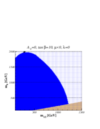
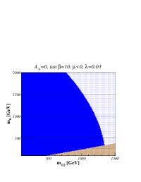
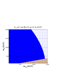
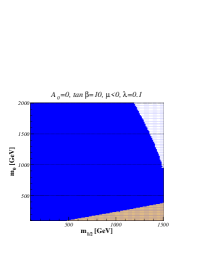
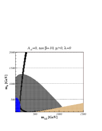
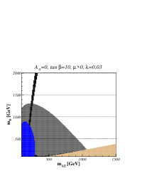
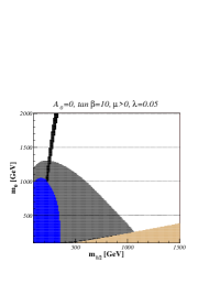
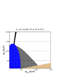
Figure 2.1: The $(m_{0},m_{1/2})$-planes for $\tan\beta=10$, $A_{0}=0$ GeV, $\mu<0$, and $\lambda=0$, 0.03, 0.05 and 0.1. We show WMAP (black) favoured as well as $b\to s\gamma$ (blue) and charged LSP (beige) excluded regions of mSUGRA parameter space in minimal ($\lambda=0$) and non-minimal ($\lambda>0$) flavour violation.

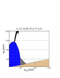
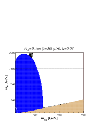
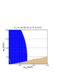
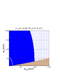
Figure 2.2: Same as Fig. 2.4, for $\tan\beta=10$, $A_{0}=0$ GeV, $\mu>0$, and $\lambda=0$, 0.03, 0.05 and 0.1.

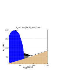
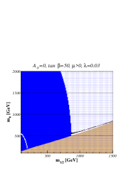
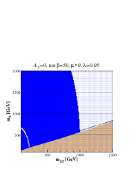
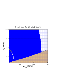
Figure 2.3: Same as Fig. 2.4, for $\tan\beta=30$, $A_{0}=0$ GeV, $\mu>0$, and $\lambda=0$, 0.03, 0.05 and 0.1.

Figure 2.4: Same as Fig. 2.4, for $\tan\beta=50$, $A_{0}=0$ GeV, $\mu>0$, and $\lambda=0$, 0.03, 0.05 and 0.1.

Typical scans of the mSUGRA parameter space in $m_{0}$ and $m_{1/2}$ with a relatively small value of $\tan\beta=10$ and $A_{0}=0$ are shown in Figs. 2.4 and 2.4 for $\mu<0$ and $\mu>0$, respectively. All experimental limits described in the previous section are imposed at the $2\sigma$-level. The $b\to s\gamma$ excluded region depends strongly on flavour mixing, while the regions favoured by $g_{\mu}-2$ and the dark matter relic density are quite insensitive to variations of the $\lambda$-parameter. $\Delta\rho$ constrains the parameter space only for heavy universal scalar masses $m_{0}>2000$ GeV and heavy universal gaugino masses $m_{1/2}>1500$ GeV, so that the corresponding excluded regions are not shown here. The dominant SUSY effects in the calculation of the anomalous magnetic moment of the muon come from induced quantum loops of a neutralino or a chargino and a slepton, while squarks contribute only at the two-loop level. This reduces the dependence on flavour violation in the squark sector considerably. Furthermore, the region $\mu<0$ is disfavoured in all SUSY models, since the one-loop SUSY contributions are approximatively given by [158]

$$a_{\mu}^{{\rm SUSY,\leavevmode\nobreak\ 1-loop}}\simeq 13\times 10^{-10}\,\left(\frac{100\leavevmode\nobreak\ {\rm GeV}}{M_{\rm SUSY}}\right)^{2}\tan\beta\ {\rm sgn}(\mu),$$ (2.99)

where $M_{\rm SUSY}$ is a typical SUSY mass scale. Negative values of $\mu$ would then increase, not decrease, the disagreement between the experimental measurements and the theoretical value of $a_{\mu}$. Furthermore, the measured $b\to s\gamma$ branching ratio excludes virtually all of the region favoured by the dark matter relic density, except for very high scalar SUSY masses. We therefore do not consider negative values of $\mu$ in the rest of this work.

In Figs. 2.4 and 2.4, we show the ($m_{0},m_{1/2}$)-planes for larger $\tan\beta$, namely $\tan\beta=30$ and $\tan\beta=50$, and for $\mu>0$. The regions which are favoured both by the anomalous magnetic moment of the muon and by the cold dark matter relic density, and which are not excluded by the $b\to s\gamma$ measurements, are stringently constrained and do not allow for large flavour violation.

2.3.4 NMFV benchmark points and slopes

Restricting ourselves to non-negative values of $\mu$, we now inspect the $(m_{0},m_{1/2})$-planes in Figs. 2.4-2.4 for scenarios that are allowed or favoured by low-energy, electroweak precision, and cosmological constraints, that permit non-minimal flavour violation among left-chiral squarks of the second and third generation up to $\lambda\lesssim 0.1$, and that are at the same time collider-friendly, with relatively low values of $m_{0}$ and $m_{1/2}$. We propose [97] the four benchmark points given in Tab. 2.3. We also attach a model line (slope) to each point in Tab. 2.4. These slopes trace the allowed/favoured regions from lower to higher masses and can, of course, also be used in MFV scenarios where the off-diagonal terms are expressed in function of the CKM matrix and the Yukawa couplings, and in cMFV with $\lambda=0$.

Table 2.3: Benchmark points allowing for flavour violation among the second and third generations for $A_{0}=0$, $\mu>0$, and three different values of $\tan\beta$.

	$m_{0}$ [GeV]	$m_{1/2}$ [GeV]	$A_{0}$ [GeV]	$\tan\beta$	sgn($\mu$)
A	700	200	0	10	1
B	100	400	0	10	1
C	230	590	0	30	1
D	600	700	0	50	1

Table 2.4: Model lines allowing for flavour violation among the second and third generations for $A_{0}=0$, $\mu>0$, and three different values of $\tan\beta$.

A	$180\leavevmode\nobreak\ {\rm GeV}\leavevmode\nobreak\ \leq\leavevmode\nobreak\ m_{1/2}\leavevmode\nobreak\ \leq\leavevmode\nobreak\ 250\leavevmode\nobreak\ {\rm GeV}\leavevmode\nobreak\ ,$	$m_{0}\leavevmode\nobreak\ =\leavevmode\nobreak\ \leavevmode\nobreak\ -1936\leavevmode\nobreak\ {\rm GeV}+\leavevmode\nobreak\ 12.9\,m_{1/2},\leavevmode\nobreak\$
B	$400\leavevmode\nobreak\ {\rm GeV}\leavevmode\nobreak\ \leq\leavevmode\nobreak\ m_{1/2}\leavevmode\nobreak\ \leq\leavevmode\nobreak\ 900\leavevmode\nobreak\ {\rm GeV}\leavevmode\nobreak\ ,$	$m_{0}\leavevmode\nobreak\ =\leavevmode\nobreak\ \leavevmode\nobreak\ \leavevmode\nobreak\ \leavevmode\nobreak\ \leavevmode\nobreak\ 4.93\leavevmode\nobreak\ {\rm GeV}+0.229\,m_{1/2},\leavevmode\nobreak\$
C	$500\leavevmode\nobreak\ {\rm GeV}\leavevmode\nobreak\ \leq\leavevmode\nobreak\ m_{1/2}\leavevmode\nobreak\ \leq\leavevmode\nobreak\ 700\leavevmode\nobreak\ {\rm GeV}\leavevmode\nobreak\ ,$	$m_{0}\leavevmode\nobreak\ =\leavevmode\nobreak\ \leavevmode\nobreak\ \leavevmode\nobreak\ \leavevmode\nobreak\ \leavevmode\nobreak\ \leavevmode\nobreak\ \leavevmode\nobreak\ \,54\leavevmode\nobreak\ {\rm GeV}+0.297\,m_{1/2},\leavevmode\nobreak\$
D	$575\leavevmode\nobreak\ {\rm GeV}\leavevmode\nobreak\ \leq\leavevmode\nobreak\ m_{1/2}\leavevmode\nobreak\ \leq\leavevmode\nobreak\ 725\leavevmode\nobreak\ {\rm GeV}\leavevmode\nobreak\ ,$	$m_{0}\leavevmode\nobreak\ =\leavevmode\nobreak\ \leavevmode\nobreak\ \leavevmode\nobreak\ \leavevmode\nobreak\ \leavevmode\nobreak\ \leavevmode\nobreak\ 600\leavevmode\nobreak\ {\rm GeV}.$

Starting with Fig. 2.4 and $\tan\beta=10$, the bulk region of equally low scalar and fermion masses is all but excluded by the $b\to s\gamma$ branching ratio. This leaves us with two favoured regions. Our benchmark point A lies in the so-called focus point region of low fermion masses $m_{1/2}$, where the lightest neutralinos are relatively heavy, have a significant Higgsino component, and annihilate dominantly into pairs of electroweak gauge bosons. Our values for the universal masses are smaller than those of the pre-WMAP point SPS 2 [45, 46] ($m_{0}=1450$ GeV, $m_{1/2}=300$ GeV) and post-WMAP point BDEGOP E’ [159] ($m_{0}=1530$ GeV, $m_{1/2}=300$ GeV), which lie outside the region favoured by $a_{\mu}$ (grey-shaded) and lead to collider-unfriendly heavy squark and gaugino masses. Our benchmark point B lies in the co-annihilation branch of low scalar masses $m_{0}$, where the lighter $\tilde{\tau}_{1}$ mass eigenstate is not much heavier than the lightest neutralino, the two having a considerable co-annihilation cross section. This point differs from the points SPS 3 ($m_{0}=90$ GeV, $m_{1/2}=400$ GeV) and BDEGOP C’ ($m_{0}=85$ GeV, $m_{1/2}=400$ GeV) only very little in the scalar mass.

At the larger value of $\tan\beta=30$ in Fig. 2.4, only the co-annihilation region survives the constraints coming from $b\to s\gamma$ decays, where we choose our point C, which has slightly higher masses than both SPS 1b ($m_{0}=200$ GeV, $m_{1/2}=400$ GeV) and BDEGOP I’ ($m_{0}=175$ GeV, $m_{1/2}=350$ GeV). Finally for the very large value of $\tan\beta=50$ in Fig. 2.4, the bulk region reappears at relatively heavy scalar and fermion masses. Here, the couplings of the heavier scalar and pseudo-scalar Higgses $H^{0}$ and $A^{0}$ to bottom quarks and tau-leptons and the charged-Higgs coupling to top-bottom pairs are significantly enhanced, resulting e.g. in increased dark matter annihilation cross sections through $s$-channel Higgs-exchange into bottom-quark final states. So as $\tan\beta$ increases further, the so-called Higgs-funnel region eventually makes its appearance on the diagonal of large scalar and fermion masses. We choose our point D in the concentrated (bulky) region favoured by cosmology and $a_{\mu}$ at masses, that are slightly higher than those of SPS 4 ($m_{0}=400$ GeV, $m_{1/2}=300$ GeV) and BDEGOP L’ ($m_{0}=300$ GeV, $m_{1/2}=450$ GeV). In this scenario, squarks and gluinos are very heavy with masses above 1 TeV.

Let us now turn to the dependence of the precision variables discussed in Sec. 2.3.2 on the flavour violating parameter $\lambda$ in our four benchmark scenarios. As already mentioned, we expect the leptonic observable $a_{\mu}$ to depend weakly on the squark sector, which is confirmed by our numerical analysis of the SUSY contribution $a_{\mu}^{(SUSY)}$. We find constant values of 6, 14, 16, and 13$\times 10^{-10}$ for the benchmarks A, B, C, and D, all of which lie well within $2\sigma$ (the latter three even within $1\sigma$) of the experimentally favoured range $(22\pm 10)\times 10^{-10}$.

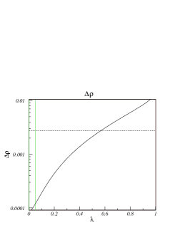
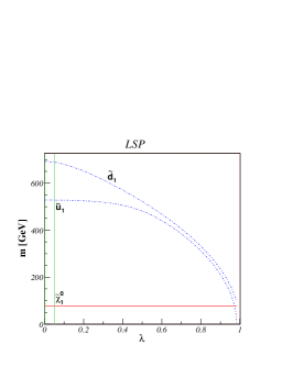
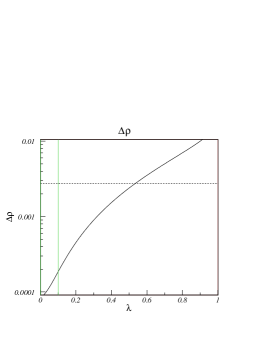
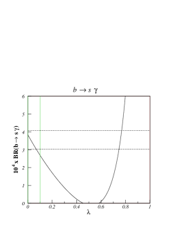
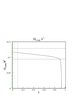
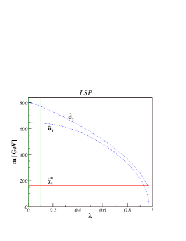
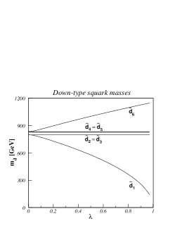
Figure 2.5: Dependence of the precision variables $\Delta\rho$, BR$(b\to s\gamma)$, and the cold dark matter relic density $\Omega_{CDM}h^{2}$ (top) as well as of the lightest SUSY particle, up- and down-type squark masses (bottom) on the NMFV parameter $\lambda$ in our benchmark scenario A. The experimentally allowed ranges (within $2\sigma$) are indicated by horizontal dashed lines.

Figure 2.6: Same as Fig. 2.6 for our benchmark scenario B.

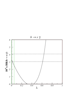
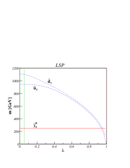
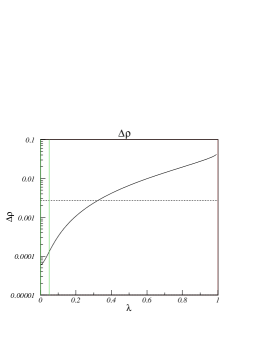
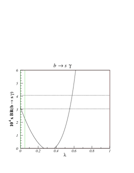
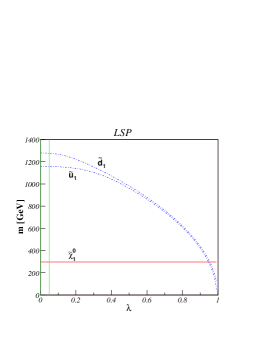
Figure 2.7: Same as Fig. 2.8 for our benchmark scenario C.

Figure 2.8: Same as Fig. 2.6 for our benchmark scenario D.

The electroweak precision observable $\Delta\rho$ is shown first in Figs. 2.6-2.8 for the four benchmark scenarios, where only the experimental upper bound of the $2\sigma$-range is visible as a dashed line. While the self-energy diagrams of the electroweak gauge bosons depend obviously strongly on the helicities, flavours, and mass eigenvalues of the squarks in the loop, the SUSY masses in our scenarios are sufficiently small and the experimental error is still sufficiently large to allow for relatively large values of $\lambda\leq 0.57$, 0.52, 0.38, and 0.32 for the benchmark points A, B, C, and D, respectively. As mentioned above, $\Delta\rho$ conversely constrains SUSY models in cMFV ($\lambda=0$) only for masses above 2000 GeV for $m_{0}$ and 1500 GeV for $m_{1/2}$.

The next diagram in Figs. 2.6-2.8 shows the dependence of the most stringent low-energy constraint, coming from the good agreement between the measured $b\to s\gamma$ branching ratio and the two-loop SM prediction, on the NMFV parameter $\lambda$. The dashed lines of the $2\sigma$-bands exhibit two allowed regions, one close to $\lambda=0$ (vertical green line) and a second one around $\lambda\simeq 0.57$, 0.75, 0.62, and 0.57, respectively. As is well-known, the latter are, however, disfavoured by $b\to s\mu^{+}\mu^{-}$ data constraining the sign of the $b\to s\gamma$ amplitude to be the same as in the SM [160]. We will therefore limit ourselves later to the regions $\lambda\leq 0.05$ (points A, C, and D) and $\lambda\leq 0.1$ (point B) in the vicinity of cMFV.

The 95% confidence-level (or $2\sigma$) region for the cold dark matter density is shown as a dashed band in the upper right part of Figs. 2.6-2.8. However, only the lower bound (0.094) is of relevance, as the relic density falls with increasing $\lambda$. This is not so pronounced in our model B as in our model A, where squark masses are light and the lightest neutralino has a sizable Higgsino-component, so that squark exchanges contribute significantly to the annihilation cross sections. For models C and D there is little sensitivity of $\Omega_{CDM}h^{2}$ (except at very large $\lambda$), as the squark masses are generally larger. The rapid fall-off of the relic density for very large $\lambda\lesssim 1$ can be understood by looking at the resulting lightest up- and down-type squark mass eigenvalues in the lower left part of Figs. 2.6-2.8. For maximal flavour violation, the off-diagonal squark mass matrix elements are of similar size as the diagonal ones, leading to one squark mass eigenvalue that approaches and finally falls below the lightest neutralino (dark matter) mass. Light squark propagators and co-annihilation processes thus lead to a rapidly falling dark matter relic density and finally to cosmologically excluded NMFV SUSY models, since the LSP is assumed to be electrically neutral and a colour singlet.

An interesting phenomenon of level reordering between neighbouring states can be observed in the lower central diagrams of Figs. 2.6-2.8 for the two lowest mass eigenvalues of up-type squarks. As $\lambda$ and the off-diagonal entries in the mass matrix increase, the splitting between the lightest and highest mass eigenvalues naturally increases. It is first the second-lowest mass that decreases up to intermediate values of $\lambda=0.2...0.5$, whereas the lowest mass is constant, and only at this point the second-lowest mass becomes constant and takes approximately the value of the until here lowest squark mass, whereas the lowest squark mass starts to decrease further with $\lambda$. These “avoided crossings” are a common phenomenon for Hermitian matrices and reminiscent of meta-stable systems in quantum mechanics. At the point where the two levels should cross, the corresponding squark eigenstates mix and change character. This level-reordering phenomenon occurs also for other scenarios, as well as for down-type squarks, even if it is not so pronounced for the latter, as shown in the lower right diagrams of Figs. 2.6-2.8.

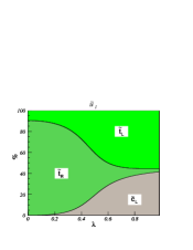
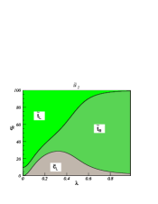
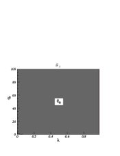
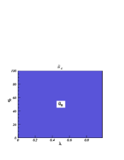
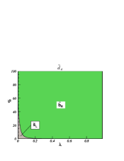
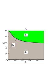
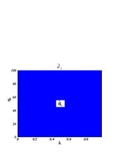
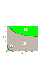
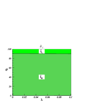
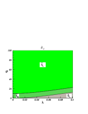
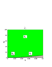
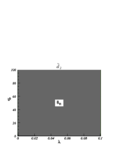
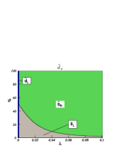
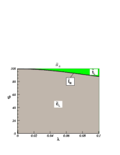
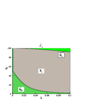
Figure 2.9: Dependence of the chirality (L, R) and flavour ($u$, $c$, $t$; $d$, $s$, and $b$) content of up- ($\tilde{u}_{i}$) and down-type ($\tilde{d}_{i}$) squark mass eigenstates on the NMFV parameter $\lambda\in[0;1]$ for benchmark point A.

Figure 2.10: Same as Fig. 2.10 for $\lambda\in[0;0.1]$.

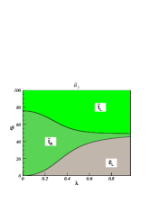
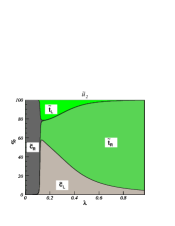
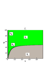
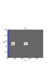
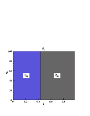
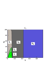
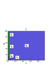
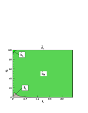
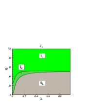
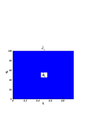
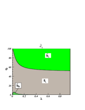
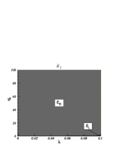
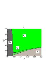
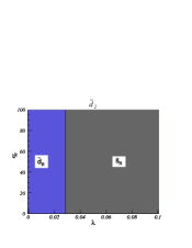
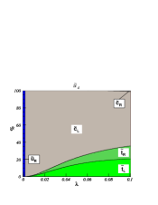
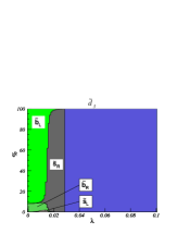
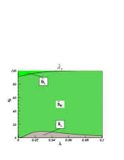
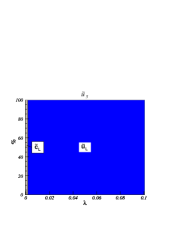
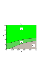
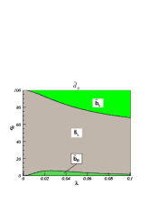
Figure 2.11: Same as Fig. 2.10 for benchmark point B.

Figure 2.12: Same as Fig. 2.12 for $\lambda\in[0;0.1]$.

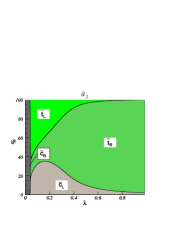
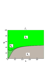
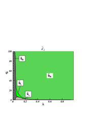
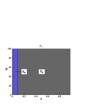
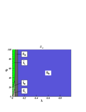
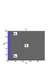
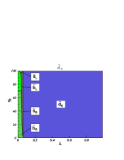
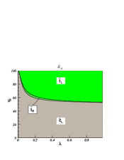
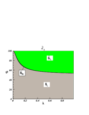
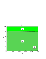
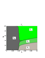
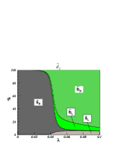
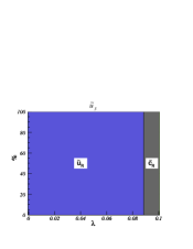
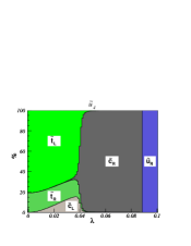
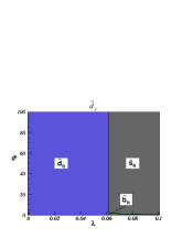
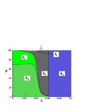
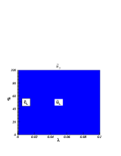
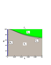
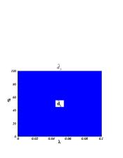
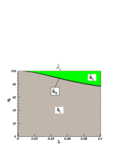
Figure 2.13: Same as Fig. 2.10 for benchmark point C.

Figure 2.14: Same as Fig. 2.14 for $\lambda\in[0;0.1]$.

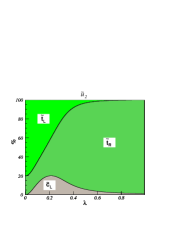
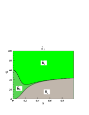
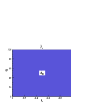
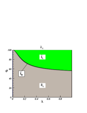
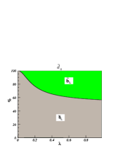
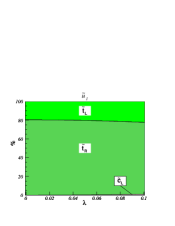
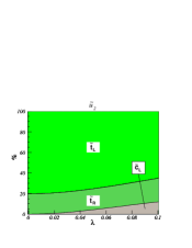
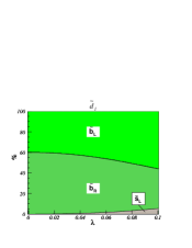
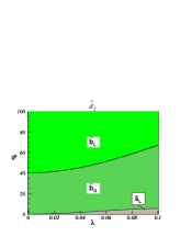
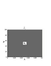
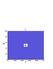
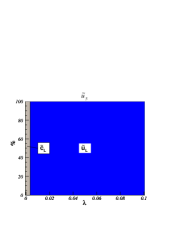
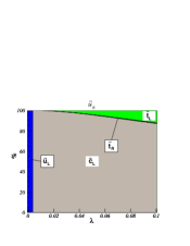
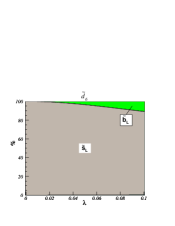
Figure 2.15: Same as Fig. 2.10 for benchmark point D.

Figure 2.16: Same as Fig. 2.16 for $\lambda\in[0;0.1]$.

As shown in Eq. (2.88) in NMFV, squarks exhibit mixing of left- and right-handed helicities and the three generations. For our benchmark scenario A, the helicity and flavour decomposition of the six up-type (left) and down-type (right) squark mass eigenstates is shown in Fig. 2.10 for the full range of the parameter $\lambda\in[0;1]$ and in Fig. 2.10 for the experimentally favoured range in the vicinity of MFV, $\lambda\in[0;0.1]$. Left- and right-handed first-generation and right-handed second-generation squarks remain, of course, helicity- and flavour-diagonal, with the left-handed and first-generation squarks being slightly heavier due their weak isospin coupling (see Eqs. (2.39), (2.40) and (2.43)) and different renormalization-group running effects. The lightest up-type squark $\tilde{u}_{1}$ remains the traditional mixture of left- and right-handed stops over a large region of $\lambda\leq 0.4$, but it shows at this point the flavour transition expected from the level reordering phenomenon (central plot of Fig. 2.6). The transition happens, however, above the experimental limit of $\lambda\leq 0.1$. Below this limit, it is the states $\tilde{u}_{2}$, $\tilde{u}_{6}$, $\tilde{d}_{1}$, and in particular $\tilde{d}_{4}$ and $\tilde{d}_{6}$ that show, in addition to helicity mixing, the most interesting and smooth variation of second- and third-generation flavour content (see Fig. 2.10). Note that at very low $\lambda\simeq 0.002$ the states $\tilde{d}_{L}$ and $\tilde{s}_{L}$ rapidly switch levels.

For the benchmark point B, whose helicity and flavour decomposition is shown in Fig. 2.12, level reordering occurs at $\lambda\simeq 0.4$ for the intermediate-mass up-type squarks. Close inspection of Fig. 2.12 shows, however, that also $\tilde{d}_{R}$ and $\tilde{s}_{R}$ switch levels at low values of $\lambda\simeq 0.02$. At $\lambda\simeq 0.01$, in addition $\tilde{s}_{R}$ and $\tilde{b}_{L}$ switch levels, and at $\lambda\simeq 0.002$ it is the states $\tilde{u}_{L}$ and $\tilde{c}_{L}$. The lightest up-type squark is again nothing but a mix of left- and right-handed stops up to $\lambda\leq 0.4$. Phenomenologically smooth transitions below $\lambda\leq 0.1$ involving taggable third-generation squarks are observed for $\tilde{u}_{4}$, $\tilde{u}_{6}$, $\tilde{d}_{1}$, and $\tilde{d}_{6}$.

For our scenario C, shown in Fig. 2.14, just below $\lambda=0.1$, $\tilde{u}_{R}$ and $\tilde{c}_{R}$ as well as $\tilde{d}_{R}$ and $\tilde{s}_{R}$ rapidly switch levels, and $\tilde{u}_{L}$ and $\tilde{c}_{L}$ switch levels at very low $\lambda\simeq 0.002$. These changes were already visible upon close inspection of the lower central and right plots in Fig. 2.8. On the other hand, the lightest squarks $\tilde{u}_{1}$ and $\tilde{d}_{1}$ only acquire significant flavour admixtures at relatively large $\lambda\simeq 0.2...0.4$, whereas they are mostly superpositions of left- and right-handed stops and sbottoms in the experimentally favourable range of $\lambda\leq 0.1$ shown in Fig. 2.14. Here, the heaviest $\tilde{u}_{6}$ and $\tilde{d}_{6}$ show already smooth admixtures of third-generation squarks as it was the case for the scenarios A and B discussed above. The most interesting states are $\tilde{u}_{2}$, $\tilde{u}_{4}$, $\tilde{d}_{2}$, and $\tilde{d}_{4}$, respectively, since they represent combinations of up to four different helicity and flavour states and have a significant, taggable third-generation flavour content.

The helicity and flavour decomposition for our scenario D, shown in Fig. 2.16, is rather similar to the one in scenario A, and only the mixed down-type state $\tilde{d}_{4}$ is now lighter and becomes $\tilde{d}_{2}$. The lightest up-type squark $\tilde{u}_{1}$ is again mostly a mix of left- and right-handed top squarks up to $\lambda\simeq 0.4$, where the level reordering and generation mixing occurs (see lower central part of Fig. 2.8). At the experimentally favoured lower value of $\lambda\leq 0.1$, the states $\tilde{u}_{2}$, $\tilde{d}_{1}$, $\tilde{d}_{2}$, and $\tilde{d}_{6}$ exhibit some smooth variations, shown in detail in Fig. 2.16, albeit to a lesser extent than in scenario A. At very low $\lambda\simeq 0.004$, it is now the up-type squarks $\tilde{u}_{L}$ and $\tilde{c}_{L}$ that rapidly switch levels.

2.4 Generalized couplings

Considering the strong interaction first, it is well known that the interaction of quarks, squarks, and gluinos can in general lead to flavour violation in the left- and right-handed sectors through non-diagonal entries in the matrices $R^{q}$,

$$\left\{L_{\tilde{q}_{j}q_{k}\tilde{g}},R_{\tilde{q}_{j}q_{k}\tilde{g}}\right\} = \left\{R^{q}_{jk},-R^{q}_{j(k+3)}\right\}.\leavevmode\nobreak\$$ (2.100)

Of course, the involved quark and squark both have to be up- or down-type, since the gluino is electrically neutral.

For the electroweak interaction, we define the square of the weak coupling constant $g_{W}^{2}=e^{2}/\sin^{2}\theta_{W}$ in terms of the electromagnetic fine structure constant $\alpha=e^{2}/(4\pi)$ and the squared sine of the electroweak mixing angle $x_{W}=\sin^{2}\theta_{W}=s_{W}^{2}=1-\cos^{2}\theta_{W}=1-c_{W}^{2}$. The $W^{\pm}-\tilde{\chi}^{0}_{i}-\tilde{\chi}^{\pm}_{j}$, $Z-\tilde{\chi}^{+}_{i}-\tilde{\chi}^{-}_{j}$, and $Z-\tilde{\chi}^{0}_{i}-\tilde{\chi}^{0}_{j}$ interactions are proportional to [22]

$$O^{L}_{ij}=-\frac{1}{\sqrt{2}}N_{i4}V^{\ast}_{j2}+N_{i2}V^{\ast}_{j1} {\rm and} O^{R}_{ij}=\frac{1}{\sqrt{2}}N_{i3}^{\ast}U_{j2}+N_{i2}^{\ast}U_{j1},\leavevmode\nobreak\$$ (2.101)

$$O^{\prime L}_{ij}=-V_{i1}V_{j1}^{\ast}-\frac{1}{2}V_{i2}V_{j2}^{\ast}+\delta_{ij}x_{W} {\rm and} O^{\prime R}_{ij}=-U_{i1}^{\ast}U_{j1}-\frac{1}{2}U_{i2}^{\ast}U_{j2}+\delta_{ij}x_{W},\leavevmode\nobreak\ \leavevmode\nobreak\ \leavevmode\nobreak\ \leavevmode\nobreak\ \leavevmode\nobreak\ \leavevmode\nobreak\$$ (2.102)

$$O^{\prime\prime L}_{ij}=-\frac{1}{2}N_{i3}N_{j3}^{\ast}+\frac{1}{2}N_{i4}N_{j4}^{\ast} {\rm and} O^{\prime\prime R}_{ij}=\frac{1}{2}N_{i3}^{\ast}N_{j3}-\frac{1}{2}N_{i4}^{\ast}N_{j4}\leavevmode\nobreak\ .$$ (2.103)

In NMFV, the coupling strengths of left- and right-handed (s)quarks to the electroweak gauge bosons are given by

$$\{L_{qq^{\prime}Z},R_{qq^{\prime}Z}\} = (2\,T^{3}_{q}-2\,e_{q}\,x_{W})\times\delta_{qq^{\prime}},\leavevmode\nobreak\$$ (2.104)

$$\{L_{\tilde{q}_{i}\tilde{q}_{j}Z},R_{\tilde{q}_{i}\tilde{q}_{j}Z}\} = (2\,T^{3}_{\tilde{q}}-2\,e_{\tilde{q}}\,x_{W})\times\sum_{k=1}^{3}\{R^{u}_{ik}\,R^{u\ast}_{jk},R^{u}_{i(3+k)}\,R^{u\ast}_{j(3+k)}\},\leavevmode\nobreak\$$ (2.105)

$$\{L_{qq^{\prime}W},R_{qq^{\prime}W}\} = \{\sqrt{2}\,c_{W}\,V_{qq^{\prime}},0\},\leavevmode\nobreak\$$ (2.106)

$$\{L_{\tilde{u}_{i}\tilde{d}_{j}W},R_{\tilde{u}_{i}\tilde{d}_{j}W}\} = \sum_{k,l=1}^{3}\{\sqrt{2}\,c_{W}\,V_{u_{k}d_{l}}\,R^{u}_{ik}\,R^{d\ast}_{jl},\,0\},$$ (2.107)

where $V_{kl}$ denotes the elements of the CKM-matrix. To simplify the notation, we have introduced flavour indices in the latter, $d_{1}=d$, $d_{2}=s$, $d_{3}=b$, $u_{1}=u$, $u_{2}=c$, and $u_{3}=t$. The SUSY counterparts of these vertices correspond to the quark-squark-gaugino couplings,

$$L_{\tilde{d}_{j}d_{k}\tilde{\chi}^{0}_{i}} = \!\!\bigg{[}(e_{q}\!-\!T^{3}_{q})\,s_{W}N_{i1}\!+\!T^{3}_{q}\,\cos\theta_{W}N_{i2}\bigg{]}R^{d\ast}_{jk}\!+\!\frac{m_{d_{k}}\!c_{W}N_{i3}R^{d\ast}_{j(k+3)}}{2\,m_{W}\cos\beta},\leavevmode\nobreak\ \leavevmode\nobreak\ \leavevmode\nobreak\ \leavevmode\nobreak\ \leavevmode\nobreak\$$ (2.108)

$$-R_{\tilde{d}_{j}d_{k}\tilde{\chi}_{i}^{0}}^{\ast} = e_{q}\,s_{W}\,N_{i1}\,R^{d}_{j(k+3)}-\frac{m_{d_{k}}c_{W}\,N_{i3}\,R^{d}_{jk}}{2\,m_{W}\,\cos\beta},\leavevmode\nobreak\ \leavevmode\nobreak\ \leavevmode\nobreak\ \leavevmode\nobreak\ \leavevmode\nobreak\$$ (2.109)

$$L_{\tilde{u}_{j}u_{k}\tilde{\chi}^{0}_{i}} = \!\!\bigg{[}(e_{q}\!-\!T^{3}_{q})\,s_{W}N_{i1}\!+\!T^{3}_{q}\,c_{W}N_{i2}\bigg{]}R^{u\ast}_{jk}\!+\!\frac{m_{u_{k}}\!c_{W}N_{i4}R^{u\ast}_{j(k+3)}}{2\,m_{W}\sin\beta},\leavevmode\nobreak\ \leavevmode\nobreak\ \leavevmode\nobreak\ \leavevmode\nobreak\ \leavevmode\nobreak\$$ (2.110)

$$-R_{\tilde{u}_{j}u_{k}\tilde{\chi}_{i}^{0}}^{\ast} = e_{q}\,s_{W}\,N_{i1}\,R^{u}_{j(k+3)}-\frac{m_{u_{k}}\,c_{W}\,N_{i4}\,R^{u}_{jk}}{2\,m_{W}\,\sin\beta},\leavevmode\nobreak\$$ (2.111)

$$L_{\tilde{d}_{j}u_{l}\tilde{\chi}_{i}^{\pm}} = \sum_{k=1}^{3}\bigg{[}U_{i1}\,R^{d\ast}_{jk}-\frac{m_{d_{k}}\,U_{i2}\,R^{d\ast}_{j(k+3)}}{\sqrt{2}\,m_{W}\,\cos\beta}\bigg{]}V_{u_{l}d_{k}},\leavevmode\nobreak\$$ (2.112)

$$-R^{\ast}_{\tilde{d}_{j}u_{l}\tilde{\chi}_{i}^{\pm}} = \sum_{k=1}^{3}\frac{m_{u_{l}}\,V_{i2}\,V_{u_{l}d_{k}}^{\ast}\,R^{d}_{jk}}{\sqrt{2}\,m_{W}\,\sin\beta},\leavevmode\nobreak\$$ (2.113)

$$L_{\tilde{u}_{j}d_{l}\tilde{\chi}_{i}^{\pm}} = \sum_{k=1}^{3}\bigg{[}V_{i1}^{\ast}\,R^{u}_{jk}-\frac{m_{u_{k}}\,V_{i2}^{\ast}\,R^{u}_{j(k+3)}}{\sqrt{2}\,m_{W}\,\sin\beta}\bigg{]}V_{u_{k}d_{l}},\leavevmode\nobreak\$$ (2.114)

$$-R^{\ast}_{\tilde{u}_{j}d_{l}\tilde{\chi}_{i}^{\pm}} = \sum_{k=1}^{3}\frac{m_{d_{l}}\,U_{i2}^{\ast}V_{u_{k}d_{l}}^{\ast}\,R^{u\ast}_{jk}}{\sqrt{2}\,m_{W}\,\cos\beta}\leavevmode\nobreak\ .$$ (2.115)

These general expressions can be simplified by neglecting the Yukawa couplings except for the one of the top quark, whose mass is not small compared to $m_{W}$. The usual MSSM couplings, and the couplings involving sleptons and sneutrinos are easily obtained by replacing the mixing matrices, the masses, and the CKM matrix in a proper way from the above equations.

Chapter 3 Resummation formalisms

3.1 General points

3.1.1 Main features of the resummation procedure

The finite energy or angular resolution of any particle detector implies that physical cross sections are always inclusive over arbitrarily soft produced particles. For example, a single quark jet cannot be distinguished from a quark jet accompanied by some collinear gluons or by partons with vanishing momentum. This implies that after the renormalization procedure, the remaining divergences in any physical observable are soft (due to parton radiation with small four-momentum) and/or collinear (due to emission of partons moving in parallel to the emitting one).

In fixed-order perturbation theory, infrared divergences of virtual gluons are exactly cancelled by the emission of real undetected ones, but this cancellation can leave large finite terms. In specific kinematics configurations, real and virtual contributions can be highly unbalanced, spoiling the cancellation mechanism, and only resummation to all order restores the balance. At the exclusive boundary of the phase space, when for example the tagged final state carries almost all the available energy or when its transverse momentum tends to zero, the real emission is strongly suppressed, producing a loss of balance with the virtual contribution, and spreads out up to the phase space kinematical limits through finite logarithmic terms $L$ which become large.

Let us take a given physical observable $R$, whose perturbative expansion in the strong coupling constant $\alpha_{s}$ is

$$R = R_{0}\Bigg{[}1+\sum_{n=1}^{\infty}\alpha_{s}^{n}\left(c_{2n}^{(n)}L^{2n}+c_{2n-1}^{(n)}L^{2n-1}+\ldots\right)\Bigg{]}.\leavevmode\nobreak\$$ (3.1)

The logarithmic corrections $L$ can be large even if $\alpha_{s}$ is small, enhancing thus the coefficients of the perturbative expansion. The ratio of two successive terms in Eq. (3.1) is $\mathcal{O}(\alpha_{s}L^{2})$, which means that any higher order contribution is $\mathcal{O}(1)$ with respect to the previous terms, and the reliability of perturbative predictions is thus spoiled. However, all-order resummation gives a satisfactory solution to this problem in the context of perturbation theory.

The key features of the resummation procedure are the dynamical and kinematical factorizations. Dynamical factorization comes from gauge invariance and unitarity and is completely general. The multi-gluon radiation amplitude factorizes, in the soft-limit, into the product of single-gluon emission probabilities. It is similar to multiple soft-photon emission in QED, apart from the fact that radiations of photons are uncorrelated, since they are electrically neutral. In QED, soft divergences related to degenerate final states cancel out after summation, as stated by the Bloch-Nordsieck theorem [161]. In general, this theorem is broken in QCD, since the collinear degeneracy leads to a divergence that does not necessary cancel out in the transition rates due to colour correlation in gluon interactions. The Kinoshita-Lee-Nauenberg theorem [162, 163] asserts that all the infrared divergences, soft and collinear, exactly cancel if the summation over initial and final degenerate states is carried out, and the resulting observables are infrared safe. Although it is not possible to sum over degenerate initial states, the corresponding uncancelled soft divergences are under control if the energy scale is high enough, because they are power-suppressed, while the QCD factorization theorem guarantees that the collinear divergences can be absorbed in the scale dependence of the parton densities, and they thus factorize from the hard-scattering process. This eventually leads to an exponentiation due to coherent rather than independent emission as in QED.

The second factorization concerns kinematics and occurs if phase space can be factorized in terms of single-parton phase spaces. It does not generally occur in the space where the shape variable is defined, because it depends in a complicated way on the multi-parton configuration, but rather in a conjugate space introduced via Mellin or Fourier transformation, in which momentum conservation is more easily implemented.

Both factorizations lead to exponentiation, and the observable $R$ defined in Eq. (3.1) can be rewritten as

$$R = R_{0}\exp\Bigg{[}\sum_{n=1}^{\infty}\alpha_{s}^{n}\sum_{m=1}^{n+1}G_{nm}L^{m}\Bigg{]}$$ (3.2)

$$= R_{0}\exp\Bigg{[}L\,g_{1}(\alpha_{s}L)+g_{2}(\alpha_{s}L)+\alpha_{s}\,g_{3}(\alpha_{s}L)+\ldots\Bigg{]}\leavevmode\nobreak\ ,$$

where each $g_{i}$ function corresponds to the resummation of a specific class of logarithms and contains all QCD effects due to gluon colour charge and running coupling. The ratio of two successive terms is now $\mathcal{O}(1/L)$, and the perturbative expansion is converging in the $L\gg 1$ region, provided that $\alpha_{s}L\ll 1$. All the $\alpha_{s}L^{m}$ terms with $n+1<m\leq 2n$ appearing in Eq. (3.1) are taken into account by the exponentiation of the lowest order terms and reappear in the expansion of the exponent at a given power of $\alpha_{s}$.

3.1.2 Soft-photon resummation in QED

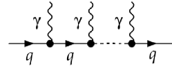
Figure 3.1: Emission of $n$ soft photons of momenta $q_{i}$.

Let us first describe multiple soft-photon emission in QED and its exponentiation [53, 164] with a generic process $f_{1}(p_{1})\,\bar{f}_{2}(p_{2})\rightarrow F(M)+X$, describing the production of a final state $F$ of mass $M$, plus some unobserved states $X$ relative to the number of emitted photons. The one-photon emission partonic cross section ${\rm d}\sigma^{(1)}(M;q)$, where $q$ is the photon momentum, is given by the product of Born cross section ${\rm d}\sigma^{(0)}(M)$ and the single photon emission probability ${\rm d}w^{(1)}(q)$

$${\rm d}\sigma^{(1)}(M;q) = {\rm d}\sigma^{(0)}(M)\,{\rm d}w^{(1)}(q)={\rm d}\sigma^{(0)}(M)\,\frac{\alpha}{4\pi^{2}\omega}\,\left|j(q)\right|^{2}$$ (3.3)

with restriction to fast fermions (with negligible mass with respect to their momentum) and to small photon energy $\omega$ compared to the scale $M$. $j^{\mu}(q)=\left(p_{2}^{\mu}/p_{2}\cdot q-p_{1}^{\mu}/p_{1}\cdot q\right)$ is the conserved emission current of a soft-photon with momentum $q$ by a fermion of momentum $p_{1}$ and antifermion of momentum $p_{2}$. The amplitude for $n$ soft-photon emissions of momenta $q_{i}$ (see Fig. 3.1) is given, in the soft-limit, by

$$M^{(n)} = \frac{e^{n}}{n!}\prod_{i=1}^{n}\frac{p_{1}\cdot\varepsilon_{i}}{q_{i}\cdot p_{1}}\leavevmode\nobreak\ ,$$ (3.4)

where $\varepsilon_{i}$ is the polarization vector of the $i^{{\rm th}}$ photon. By summing over the different polarization states, we see that the squared matrix element factorizes

$${\rm d}\sigma^{(n)}(M;q_{1},\ldots,q_{n}) = {\rm d}\sigma^{(0)}(M)\,\frac{1}{n!}\,\prod_{i=1}^{n}{\rm d}w^{(1)}(q_{i}).\leavevmode\nobreak\$$ (3.5)

This means that soft-photon emission is uncorrelated and that infrared singularities exponentiate. Indeed, kinematical factorization occurs naturally in impact-parameter $b$ space, $b$ being conjugate to the shape variable, where the $\delta$-function implementing four-momentum conservation exponentiates. Summing Eq. (3.5) to all orders, we get

$${\rm d}\sigma\,(M) = {\rm d}\sigma^{(0)}(M)\sum_{n}\int\frac{1}{n!}{\rm d}w^{(1)}(q_{1})\ldots{\rm d}w^{(n)}(q_{n})\,\delta\left(\sum_{i}q_{i}+P-p_{1}-p_{2}\right)$$ (3.6)

$$= {\rm d}\sigma^{(0)}(M)\int\frac{{\rm d}^{4}b}{(2\pi)^{4}}e^{ib\cdot(P-p_{1}-p_{2})}\sum_{n}\left[\frac{1}{n!}\int{\rm d}\tilde{w}^{(1)}(q)\,e^{iq\cdot b}\right]^{n}$$

$$= {\rm d}\sigma^{(0)}(M)\int\frac{{\rm d}^{4}b}{(2\pi)^{4}}e^{ib\cdot(P-p_{1}-p_{2})}\,\exp\left[\int{\rm d}\tilde{w}^{(1)}(q)\,e^{iq\cdot b}\right],\leavevmode\nobreak\$$

where ${\rm d}\tilde{w}$ is the Fourier transform of the single-photon emission probability ${\rm d}w$ and $P$ the four-momentum of the final state $F$. By using the usual expression of ${\rm d}\tilde{w}$ and performing the integral, we can deduce an exponentiated form factor, containing all the logarithms.

3.1.3 Soft-gluon resummation in QCD

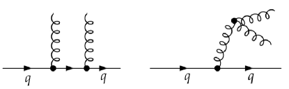
Figure 3.2: Emission of two soft-gluons.

Contrary to photons which are electrically neutral, gluons carry colour charge. However, the infrared divergences related to gluon correlations cancel among themselves and an exponentiation is still possible [165, 166]. Considering the same generic process as in the previous section, the cross section for single-gluon emission can be written as in Eq. (3.3), provided that we introduce colour operators,

$${\rm d}\sigma^{(1)}(M;q)={\rm d}\sigma^{(0)}(M)\,{\rm d}w^{(1)}(q)={\rm d}\sigma^{(0)}(M)\,\frac{\alpha_{s}}{4\pi^{2}\omega}\,\left|J^{a}(q)\right|^{2},\leavevmode\nobreak\$$ (3.7)

where $\omega$ ($q$) denotes the gluon energy (momentum) and the current $J_{\mu}^{a}(q)=T^{a}_{p_{2}}j_{\mu}(q)$ includes now the colour charge operator $T^{a}_{p_{2}}$.

For the emission of $n$ soft-gluons of momentum $q_{i}$ and energy $\omega_{i}$, diagrams where gluons are emitted by harder ones have to be taken into account, as in Fig. 3.2 for a two-gluon emission. The difference with QED comes from the second diagram, not present in the case of photons. If we assume strong ordering in gluon energies $\omega_{1}\ll\omega_{2}\ll\ldots\ll\omega_{n}\ll M$, the use of the soft limit is justified, and we can recursively define the amplitude $M^{(n)}$, since the emission of the softest gluon factorizes

$$\langle a_{1},\ldots,a_{n}\mid M^{(n)}\rangle=\langle a_{2},\ldots,a_{n}\mid J_{\mu_{1}}^{a_{1}}(q_{1})\mid b_{1},\ldots,b_{n-1}\rangle\,\langle b_{1},\ldots,b_{n-1}\mid M^{(n-1)}\rangle,\leavevmode\nobreak\$$ (3.8)

where we sum over repeated indices and where $a_{i}$ ($\mu_{i}$) are the colour (Lorentz) indices of the emitted gluons. $M^{(n)}$ can then be computed through an iterative insertion scheme, and performing the summation over $n$ leads to the exponentiation of the gluonic radiations. As an example, we will show the exponentiation of the gluon coherent state operator, whose application on the vacuum leads to the usual resummation formulas, given e.g. in [167] for transverse-momentum resummation, in [64] for threshold resummation, and in [75] for joint resummation in the case of Drell-Yan lepton pair production.

Let us consider the emission of two gluons. Using the usual definition of the current $\mathbf{J}_{\mu}(q_{1})=\sum_{i=2}^{n}\mathbf{T}_{i}\frac{{q_{i}}_{\mu}}{q_{i}\cdot q_{1}}+\mathbf{T}_{0}\,j_{\mu}(q)$ where the index $0$ labels the hard $f_{1}\bar{f}_{2}$ contribution, we get

$$\langle a_{1},a_{2}\!\mid\!M^{(2)}\rangle = \langle a_{2}\!\mid\!T_{0}^{a_{1}}\,\varepsilon_{1}\!\cdot\!j(q_{1})\!\mid\!b_{1}\rangle\langle b_{1}\!\mid\!M^{(1)}\rangle+\langle a_{2}\!\mid\!T^{a_{1}}_{2}\frac{\varepsilon_{1}\cdot q_{2}}{q_{2}\cdot q_{1}}\!\mid\!b_{1}\rangle\langle b_{1}\!\mid\!M^{(1)}\rangle$$ (3.9)

$$= C_{(1)}^{a_{1}}C_{(1)}^{a_{2}}+C_{(2)}^{a_{1}a_{2}},\leavevmode\nobreak\$$

after the introduction of the polarization vectors in Eq. (3.8). The correlation operators $C$ are recursively defined by

$$C_{(1)}^{a_{i}} = \langle a_{i}\mid M^{(1)}\rangle=\langle b\mid T_{0}^{a_{i}}\varepsilon_{i}\cdot j(q)\mid b\rangle$$

$$C_{(n)}^{a_{1}\ldots a_{n}} = \langle a_{2}\ldots a_{n}\mid\sum_{j=2}^{n}T^{a_{1}}_{j}\frac{\varepsilon_{1}\cdot q_{j}}{q_{j}\cdot q_{1}}\mid b_{1}\ldots b_{n-1}\rangle\,C_{(n-1)}^{b_{1}\ldots b_{n-1}}.\leavevmode\nobreak\$$ (3.10)

The first term of Eq. (3.9) corresponds to the emission of the softest gluon by one of the external legs (left diagram of Fig. 3.2), and the second to the emission by the harder gluon (right diagram of Fig. 3.2). Generalization to any number of gluons is straightforward,

$$\langle a_{1},\ldots,a_{n}\!\mid\!M^{(n)}\rangle\!\!=\!\!\sum_{k=1}^{n}\sum_{\{n_{1},\ldots,n_{k}\}}\!\!\!\!C_{(n_{k})}\Theta_{n_{k}}\ldots C_{(n_{1})}\Theta_{n_{1}}\Theta(1,\ldots,k)\!+\!{\rm perm.},\leavevmode\nobreak\ \leavevmode\nobreak\ \leavevmode\nobreak\$$ (3.11)

where the dependence on the colour indices is not explicitly shown in order to simplify the expression. For each value of $k$, the indices $\{a_{1},\ldots,a_{n}\}$ are partitioned into $k$ classes of $n_{i}$ indices, corresponding to $k$ chains of $n_{i}$ gluons. Inside a given class, the gluons are ordered in energy through the $\Theta_{n_{i}}$ functions so that a specific gluon can only be emitted by a harder one. Eventually, the $\Theta(1,\ldots,k)$ function orders the energies of the hardest gluon of each class.

Let us now define the coherent state operator for real emission, containing the correlation structure between the emitted gluons

$$U^{M}(A^{+}) = \sum_{n=0}^{\infty}\int{\rm d}\phi^{n}\langle a_{1},\ldots,a_{n}\mid M^{(n)}\rangle A^{+a_{1}}_{\alpha_{1}}(q_{1})\ldots A^{+a_{n}}_{\alpha_{n}}(q_{n}),\leavevmode\nobreak\$$ (3.12)

where $d\phi^{(n)}={\rm d}[q_{1}]\ldots{\rm d}[q_{n}]$ is the relativistic $n$-gluon phase space and $A^{+a_{i}}_{\alpha_{i}}(q)$ the creation operator of a gluon with colour (polarization) index $a_{i}$ ($\alpha_{i}$). Eqs. (3.10) and (3.11) lead to

$$U^{M}(A^{+}) = 1+\sum_{n=1}^{\infty}\sum_{k=1}^{n}\sum_{\{n_{i}\}}\int{\rm d}\phi^{(n_{1})}\ldots{\rm d}\phi^{(n_{k})}\left[g_{s}^{n_{k}}C_{(n_{k}-1)}\Theta_{n_{k}}\big{(}\varepsilon_{k}\cdot J_{Mk}\big{)}\right]\ldots$$ (3.13)

$$\times\left[g_{s}^{n_{1}}C_{(n_{1}-1)}\Theta_{n_{1}}\big{(}\varepsilon_{1}\cdot J_{M1}\big{)}\right]A^{+(n_{k})}\ldots A^{+(n_{1})}\,\Theta(1,\ldots,k),\leavevmode\nobreak\$$

where $A^{+(n_{i})}$ is the product of $n_{i}$ gluon creation operators and $\mathbf{J}_{Mi}^{\mu_{i}}=\sum_{j=2}^{n_{i}}\mathbf{T}_{j}\frac{q_{j}^{\mu_{i}}}{q_{j}\cdot q_{i}}$. After summing over $\{n_{i}\}$, each square bracket factor reproduces the gluon coherent state operator $\mathcal{U}^{q_{i}}(A^{+})$ where $q_{i}$ is the momentum of the fastest gluon in each class. Eventually, we get exponentiation

$$U_{M}(A^{+}) = 1+\sum_{k=1}^{\infty}g_{s}^{k}\int{\rm d}[q_{1}]\ldots{\rm d}[q_{k}]\,\Theta(1,\ldots,k)\,\big{(}\varepsilon^{\alpha_{k}}\cdot J_{Mk}^{b_{k}}\big{)}\ldots\big{(}\varepsilon^{\alpha_{1}}\cdot J_{M1}^{b_{1}}\big{)}$$

$$\times\left[\mathcal{U}^{q_{k}}(A^{+})\right]_{a_{k}b_{k}}\ldots\left[\mathcal{U}^{q_{1}}(A^{+})\right]_{a_{1}b_{1}}A^{+a_{1}}_{\alpha_{1}}(q_{1})\ldots A^{+a_{k}}_{\alpha_{k}}(q_{k})$$

$$= \bar{P}_{w}\exp\Bigg{\{}g_{s}\int{\rm d}[q]\,\Theta(M-w)\,A^{+a}_{\alpha}(q)\,\left[\mathcal{U}^{q}(A^{+})\right]_{ab}\,\big{(}\varepsilon^{\alpha}\cdot J_{Mq}^{b}\big{)}\Bigg{\}}\leavevmode\nobreak\ ,\leavevmode\nobreak\$$

(3.14)

where $\bar{P}_{w}$ orders the colour matrices appearing in $J_{Mq}$ in such a way that the harder operator acts first.

Eq. (3.1.3) is not unitary, since we have only creation operators. The unitary is restored through the introduction of destruction operators, replacing $A^{+}_{\alpha}(q)$ by $\mathcal{R}_{\alpha}(q)=A^{+}_{\alpha}(q)-A_{\alpha}(q)$. It corresponds to the inclusion of the virtual corrections that we have neglected in the first place.

3.2 Transverse-momentum resummation

3.2.1 The Collins-Soper-Sterman (CSS) formalism

Let us consider the process

$$h_{1}(p_{1})\,h_{2}(p_{2})\rightarrow F(M^{2},q_{T}^{2})+X,\leavevmode\nobreak\$$ (3.15)

where two hadrons $h_{1}$ and $h_{2}$ with momenta $p_{1}$ and $p_{2}$ collide with a centre-of-mass energy $\sqrt{s_{h}}$ to produce an observed colourless final state system $F$ with a mass $M$ and a transverse momentum $q_{T}$, while $X$ is unobserved. As $F$ does not carry any colour charge, the lowest order partonic mechanism is initiated either by $q\bar{q}$ annihilation or by gluon fusion. Isolating the divergences from the fixed-order production cross section, we can derive the resummed cross section to get a finite expression for the $q_{T}$-spectrum of the system $F$.

On the basis of the QCD factorization theorem, the most general form of the differential cross section,

$$\frac{{\rm d}^{2}\sigma}{{\rm d}M^{2}{\rm d}q_{T}^{2}}\!=\!\sum_{a,b}\int_{0}^{1}\!\!{\rm d}x_{a}\,\int_{0}^{1}\!\!{\rm d}x_{b}\,f_{a/h_{1}}(x_{a};\mu_{F})\,f_{b/h_{2}}(x_{b};\mu_{F})\,\hat{\sigma}_{ab}(M,q_{T},s;\mu_{R},\mu_{F}),\leavevmode\nobreak\ \leavevmode\nobreak\ \leavevmode\nobreak\$$ (3.16)

where $s=x_{a}\,x_{b}\,s_{h}$ is the partonic centre-of-mass energy, can be computed by convoluting the hard scattering function $\hat{\sigma}_{ab}$ with universal parton densities $f_{a/h_{1}}$ and $f_{b/h_{2}}$ of partons $a,b$ in the hadrons $h_{1},h_{2}$. The PDFs depend on the longitudinal momentum fractions of the two partons $x_{a,b}$ and on the unphysical factorization scale $\mu_{F}$. The hard part $\hat{\sigma}_{ab}$ has a perturbative expansion in $\alpha_{s}(\mu_{R})$, $\mu_{R}$ being the unphysical renormalization scale,

$$\hat{\sigma}_{ab}(M,q_{T},s;\mu_{R},\mu_{F})=\sum_{n=0}^{\infty}\left(\frac{\alpha_{s}(\mu_{R})}{\pi}\right)^{n+p}\hat{\sigma}_{ab}^{(n)}(M,q_{T},s;\mu_{F}),\leavevmode\nobreak\$$ (3.17)

where $p$ is the minimum power of $\alpha_{s}$ needed for the process to occur at leading order. Isolating the divergent terms as the transverse momentum $q_{T}\to 0$, $\hat{\sigma}_{ab}^{(n)}$ can be written as [52]

$$\hat{\sigma}_{ab}^{(n)}(M,q_{T},s;\mu_{F}) = R_{ab}^{(n)}(M,q_{T},s;\mu_{F})+\hat{\sigma}_{ab}^{(n,\delta)}(M,s;\mu_{F})\,\delta(q_{T})$$ (3.18)

$$+\sum_{m=0}^{2n-1}\!\hat{\sigma}_{ab}^{(n,m)}(M,s;\mu_{F})\,\frac{\ln^{m}(M^{2}/q_{T}^{2})}{q_{T}^{2}},\leavevmode\nobreak\$$

where $R_{ab}^{(n)}$ is the regular part of the hard function, containing all the terms less singular than $\delta(q_{T}^{2})$ and $q_{T}^{-2}$ as $q_{T}\to 0$. All the logarithmically enhanced and the $\delta(q_{T}^{2})$ contributions are resummed to all orders in $\alpha_{s}$, and the remaining terms correspond to the usual perturbative series after the removal of the logarithmic and $\delta(q_{T}^{2})$ contributions.

We define then the finite component by

$$\left[\frac{{\rm d}^{2}\sigma}{{\rm d}M^{2}{\rm d}q_{T}^{2}}\right]_{{\rm fin}} = \sum_{a,b}\int_{0}^{1}{\rm d}x_{a}\,\int_{0}^{1}{\rm d}x_{b}\,f_{a/h_{1}}(x_{a};\mu_{F})\,f_{b/h_{2}}(x_{b};\mu_{F})$$ (3.19)

$$\times\sum_{n=1}^{\infty}\left(\frac{\alpha_{s}(\mu_{R})}{\pi}\right)^{n+p}R_{ab}(M,q_{T},s;\mu_{F}),\leavevmode\nobreak\$$

which is exactly the difference between the full perturbative result and its asymptote at low $q_{T}$, containing the terms which are at least as singular as $q_{T}^{-2}$ or proportional to $\delta(q_{t}^{2})$. At low $q_{T}$, we are subtracting two terms dominated by their singularities, and their difference is thus not significant. In the large-$q_{T}$ region, the asymptote does not play a significant role, and the fixed-order theory is recovered.

For the resummed component, we rather work with its Fourier transform $\tilde{W}$ with respect to the impact-parameter $b$, the variable conjugate to $q_{T}$, because as stated in the previous section, the kinematic factorization of the multiple gluon emission is more naturally performed in impact-parameter space [53, 54]. Using the singular part of the partonic cross section $\hat{\sigma}_{ab}$, i.e. the two last terms of Eq. (3.18), and Eq. (3.16), we get

$$\tilde{W}^{F}(b;M,s;\mu_{R},\mu_{F})=\sum_{a,b}\sum_{n=0}^{\infty}\left(\frac{\alpha_{s}(\mu_{R})}{\pi}\right)^{n+p}\!\!\!\!\int_{0}^{1}\!\!{\rm d}x_{a}\!\!\int_{0}^{1}\!\!{\rm d}x_{b}\,f_{a/h_{1}}(x_{a};\mu_{F})\,f_{b/h_{2}}(x_{b};\mu_{F})$$

$$\!\!\times\!\!\int\!\!{\rm d}^{2}q_{T}\,e^{-i\,\mathbf{q}_{T}\cdot\mathbf{b}}\bigg{[}\hat{\sigma}_{ab}^{(n,\delta)}(M,s;\mu_{F})\,\delta(q_{T})\!+\!\sum_{m=0}^{2n-1}\!\hat{\sigma}_{ab}^{(n,m)}(M,s;\mu_{F})\,\frac{\ln^{m}(M^{2}/q_{T}^{2})}{q_{T}^{2}}\bigg{]}.$$ (3.20)

The dependence in the two partons $a$ and $b$ factorizes, and $\tilde{W}$ obeys an evolution equation where $b$ and $M$ dependences are separated, so that Eq. (3.20) can be simplified to the usual CSS resummation formula [56, 57, 59], taking into account the coherent gluon emission described in section 3.1.1 [167]. Omitting the dependences on the unphysical scales, we get

$$\left[\frac{{\rm d}^{2}\sigma}{{\rm d}M^{2}{\rm d}q_{T}^{2}}\right]_{{\rm res}} = \sum_{a,b}\int_{0}^{1}{\rm d}x_{a}\!\int_{0}^{1}{\rm d}x_{b}\!\int{\rm d}b\frac{b}{2}J_{0}(b\,q_{T})\,f_{a/h_{1}}(x_{1};\frac{C_{3}}{b})\,f_{b/h_{2}}(x_{2};\frac{C_{3}}{b})$$ (3.21)

$$\times\tilde{W}^{F}_{ab}(b;M,s),\leavevmode\nobreak\$$

$$\tilde{W}^{F}_{ab}(b;M,s) = \sum_{c}\!\int_{0}^{1}\frac{{\rm d}z_{1}}{z_{1}}\!\int_{0}^{1}\frac{{\rm d}z_{2}}{z_{2}}\,C^{F}_{ca}(\alpha_{s}(C_{3}/b),z_{1})\,C^{F}_{\bar{c}b}(\alpha_{s}(C_{3}/b),z_{2})\,S_{c}^{F}(M,b)$$ (3.22)

$$\times\sigma_{c\bar{c}}^{({\rm LO})F}(M)\,\delta(M^{2}-z_{1}\,z_{2}\,s),\leavevmode\nobreak\$$

where $J_{0}(x)$ is the zeroth order Bessel function of the first kind. By convention, the constants $C_{1}$, $C_{2}$, and $C_{3}$ are chosen to be $C_{1}=C_{3}=b_{0}=2\,e^{-\gamma_{E}}$ and $C_{2}=1$, where $\gamma_{E}=0.5772...$ is the Euler-Mascheroni constant. $\tilde{W}^{F}$ is computed perturbatively and is the process-dependent partonic cross section. It embodies the all-order resummation of the large logarithms $\ln(M^{2}\,b^{2})$ (conjugate to $\ln M^{2}/q_{T}^{2}$), and $\sigma_{c\bar{c}}^{({\rm LO})F}$ is the total cross section for the LO partonic subprocess $c\bar{c}\to F$. The resummation of the logarithms is completely achieved by the exponentiation in the quark ($c=q$) or gluon ($c=g$) Sudakov form factor $S_{c}^{F}$, which can be expressed as [55, 56, 57, 168],

$$S^{F}_{c}(M,b)=\exp\left\{\!-\!\int_{C_{1}^{2}/b^{2}}^{C_{2}^{2}M^{2}}\!\!\frac{{\rm d}q^{2}}{q^{2}}\!\left[A_{c}(\alpha_{s}(q);C_{1})\ln\frac{C_{2}^{2}M^{2}}{q^{2}}\!+\!B^{F}_{c}(\alpha_{s}(q);C_{1},C_{2})\right]\!\right\},\leavevmode\nobreak\ \leavevmode\nobreak\$$ (3.23)

depending only on the two functions $A_{c}$, relative to soft-radiation, and $B_{c}$, relative to flavour conserving collinear radiation, and which can be perturbatively computed

$$A_{c}(\alpha_{s})=\sum_{n=1}^{\infty}\left(\frac{\alpha_{s}}{\pi}\right)^{n}A_{c}^{(n)} {\rm\leavevmode\nobreak\ \leavevmode\nobreak\ \leavevmode\nobreak\ \leavevmode\nobreak\ and\leavevmode\nobreak\ \leavevmode\nobreak\ \leavevmode\nobreak\ \leavevmode\nobreak\ } B_{c}^{F}(\alpha_{s})=\sum_{n=1}^{\infty}\left(\frac{\alpha_{s}}{\pi}\right)^{n}B_{c}^{(n)}.\leavevmode\nobreak\$$ (3.24)

The coefficients of these series can be obtained by comparing the expansion of Eq. (3.21) at a given order in $\alpha_{s}$ with the expression of the fixed-order cross section in the small-$q_{T}$ limit. The lowest order coefficients, needed for resummation at NLL accuracy, have been computed both for the quark [55, 168] and the gluon [169] form factors,

$$A_{q}^{(1)}=C_{F} {\rm\leavevmode\nobreak\ \leavevmode\nobreak\ \leavevmode\nobreak\ \leavevmode\nobreak\ and\leavevmode\nobreak\ \leavevmode\nobreak\ \leavevmode\nobreak\ \leavevmode\nobreak\ } A_{g}^{(1)}=C_{A}$$ (3.25)

$$A_{q}^{(2)}=\frac{1}{2}C_{F}\,K {\rm\leavevmode\nobreak\ \leavevmode\nobreak\ \leavevmode\nobreak\ \leavevmode\nobreak\ and\leavevmode\nobreak\ \leavevmode\nobreak\ \leavevmode\nobreak\ \leavevmode\nobreak\ } A_{g}^{(2)}=\frac{1}{2}C_{A}\,K$$ (3.26)

$$B_{q}^{(1)}=-\frac{3}{2}C_{F} {\rm\leavevmode\nobreak\ \leavevmode\nobreak\ \leavevmode\nobreak\ \leavevmode\nobreak\ and\leavevmode\nobreak\ \leavevmode\nobreak\ \leavevmode\nobreak\ \leavevmode\nobreak\ } B_{g}^{(1)}=-\frac{1}{6}\left(11C_{A}-2n_{f}\right),\leavevmode\nobreak\$$ (3.27)

where $K=\left[\left(\frac{67}{18}-\frac{\pi^{2}}{6}\right)C_{A}-\frac{5}{9}n_{f}\right]$, and where $C_{F}=4/3$ and $C_{A}=3$ are the usual QCD colour factors. The process-dependent coefficient $B_{c}^{(2)F}$ has been computed for different processes, as for example Drell-Yan pair [60] or Higgs production [170].

Finally, the $C_{ab}^{F}$ coefficient functions of Eq. (3.22) can as well be computed perturbatively

$$C_{ab}(\alpha_{s},z) = \delta_{ab}\,\delta(1-z)+\sum_{n=1}^{\infty}\left(\frac{\alpha_{s}}{\pi}\right)^{n}C_{ab}^{(n)}(z),\leavevmode\nobreak\$$ (3.28)

where $z=M^{2}/s$. They contain a collinear contribution which has its origin in the particularities of the $\overline{{\rm MS}}$ scheme, where the full splitting functions are not factorized into the parton densities, and a hard process-dependent contribution coming from the finite part of virtual-loop corrections. The first coefficient $C^{(1)}$ is known for a large number of processes [58, 60, 170, 171, 172, 173, 174, 175].

3.2.2 Non-perturbative effects in the CSS formalism

The $q_{T}$-distribution is affected by non-perturbative effects associated with the large-$b$ region, $b\gtrsim 1/\Lambda_{{\rm QCD}}$, where the strong coupling $\alpha_{s}$ and the PDFs at the scale $b_{0}/b$ enter the non-perturbative regime. To take these effects into account, the function $\tilde{W}_{ab}^{F}$ is evaluated at a new variable $b_{\ast}=b/\sqrt{1+(b/b_{{\rm max}})^{2}}$, far from the region where non-perturbative effects are relevant, the latter being included in a function $F^{{\rm NP}}$. Practically, the $\tilde{W}^{F}$ function of Eq. (3.21) is replaced by

$$\tilde{W}_{ab}^{{\rm NP}F}(b;M,x_{1},x_{2})=\tilde{W}_{ab}^{F}(b_{\ast};M,s)\,F_{ab}^{{\rm NP}}(b;M,x_{1},x_{2}).\leavevmode\nobreak\$$ (3.29)

The value of $b_{{\rm max}}$ and the shape of $F^{{\rm NP}}$ have to be chosen so that $\tilde{W}_{ab}^{{\rm NP}}(b;M,x_{1},x_{2})\simeq\tilde{W}_{ab}(b;M,s)$ when $b\lesssim b_{{\rm max}}$. In the original formalism [56, 59]

$$F_{ab}^{{\rm NP}}(b,M,x_{1},x_{2})=\exp\left[-\ln(M^{2}\,b_{{\rm max}}^{2})\,g_{1}(b)-g_{a/h_{1}}(x_{1},b)-g_{b/h_{2}}(x_{2},b)\right],\leavevmode\nobreak\$$ (3.30)

where the three $g$-functions are assumed to vanish as $b\to 0$. The predictive power of the CSS formalism relies on the universality and the scale dependence of these functions. As the PDFs, they can be evolved from a given energy until the required scale.

The main source of non-perturbative effects comes from partons with a non-zero intrinsic transverse-momentum already inside the hadron and from unresolved gluons with $q_{T}<1/b_{{\rm max}}$. Global fits of experimental Drell-Yan data allow for different forms for this non-perturbative function [60, 176, 177, 178, 179]

$$F_{ab}^{{\rm NP}(dws)}(b,M,x_{1},x_{2})\!\!\! = \!\!\!\exp\!\!\left[-b^{2}\!\!\left(g_{1}+g_{2}\ln\frac{b_{{\rm max}}M}{2}\right)\right],\leavevmode\nobreak\ \leavevmode\nobreak\ \leavevmode\nobreak\$$ (3.31)

$$F_{ab}^{{\rm NP}(ly)}(b,M,x_{1},x_{2})\!\!\! = \!\!\!\exp\!\!\left[-b^{2}\!\!\left(\bar{g}_{1}\!+\!\bar{g}_{2}\ln\frac{b_{{\rm max}}M}{2}\right)\!-\!b\,\bar{g}_{1}\,\bar{g}_{3}\,\ln(100\,x_{1}x_{2})\!\right]\!\!,\leavevmode\nobreak\ \leavevmode\nobreak\ \leavevmode\nobreak\$$ (3.32)

$$F_{ab}^{{\rm NP}(blny)}(b,M,x_{1},x_{2})\!\!\! = \!\!\!\exp\!\!\left[-b^{2}\!\!\left(\tilde{g}_{1}+\tilde{g}_{2}\ln\frac{b_{{\rm max}}M}{2}+\tilde{g}_{1}\,\tilde{g}_{3}\ln(100\,x_{1}x_{2})\right)\!\right]\!\!,\leavevmode\nobreak\ \leavevmode\nobreak\ \leavevmode\nobreak\$$ (3.33)

$$F_{ab}^{{\rm NP}(kn)}(b,M,x_{1},x_{2})\!\!\! = \!\!\!\exp\!\!\left[-b^{2}\!\!\left(a_{1}+a_{2}\ln\frac{M}{3.2{\rm GeV}}+a_{3}\ln(100\,x_{1}\,x_{2})\right)\right].\leavevmode\nobreak\ \leavevmode\nobreak\ \leavevmode\nobreak\$$ (3.34)

The most recent values of these parameters can be found in [178, 179].

3.2.3 Disadvantages of the CSS formalism

Although the Collins-Soper-Sterman resummation formalism has been used in several processes at various levels of perturbative accuracy, it presents some disadvantages, in particular regarding the process dependence of the various coefficients of Eqs. (3.21, 3.22, 3.23). For instance, the first coefficient of the $C-$functions, $C_{ab}^{(1)F}$ can be written in terms of the one-loop matrix element of the considered process [173]. Even the Sudakov form factor, supposed to be universal and to depend only on the quark or gluon nature of the emitting particles, is process-dependent through the $B_{c}^{F}$ coefficients involving also loop diagrams [170]. Moreover, the dependence on renormalization and factorization scales, parameterized through the arbitrary coefficients $C_{1}$, $C_{2}$ and $C_{3}$ does not correspond to the usual procedure followed in fixed-order perturbative calculations, and the parton distribution functions called at the scale $b_{0}/b$ rather than $\mu_{F}$ involve extrapolation in the non-perturbative region. Eventually, expanding the resummed expression at a given power in $\alpha_{s}$ in the large-$q_{T}$ region leads to unwanted factorially growing coefficients, with oscillating signs [180].

Some of the difficulties can be overcome by performing resummation in $q_{T}$-space instead of $b$-space [181, 182], but at the cost of non fulfilment of the transverse-momentum conservation [53]. However, all these problems can be avoided by using the recently proposed universal resummation formalism in $b$-space [61, 62, 183].

3.2.4 Universal resummation formalism

General expressions of the first $C$-function coefficient and of the second $B$-function coefficient show explicitly the process-dependence of these terms [170]

$$C^{(1)F}_{ab}(z) = -{\hat{P}}^{\varepsilon}_{ab}(z)+\delta_{ab}\,\delta(1-z)\left(C_{a}\,\frac{\pi^{2}}{6}+\frac{1}{2}{\cal A}_{a}(\phi)\right),\leavevmode\nobreak\$$ (3.35)

$$B_{a}^{(2)F} = -2\,\delta P_{aa}^{(2)}+\beta_{0}\left(\frac{2}{3}C_{a}\pi^{2}+{\cal A}_{a}(\phi)\right),\leavevmode\nobreak\$$ (3.36)

where ${\hat{P}}^{\varepsilon}_{ab}(z)$ is the ${\cal O}(\varepsilon)$-term in the one-loop Altarelli-Parisi splitting kernel ($\varepsilon=(4-D)/2$), $\delta P_{aa}^{(2)}$ the coefficient of the $\delta(1-z)$ term in the two-loop splitting functions, and ${\cal A}_{a}(\phi)$ is the finite part of the one-loop virtual contributions. Contrary to the universal coefficients $A_{a}^{(1)}$ and $B_{a}^{(1)}$ determined only by the Altarelli-Parisi splitting functions, $B_{a}^{(2)F}$ and $C_{ab}^{(1)F}$ contain both collinear and hard contributions, for which $\alpha_{s}$ should be evaluated at two different scales, the same scale as the parton densities $b_{0}/b$ for the process-independent collinear contribution and the hard scale $M$ for the process-dependent hard contribution.

Making the replacement

$$\sigma_{c\bar{c}}^{({\rm LO})F}(M)\to\sigma_{c\bar{c}}^{({\rm LO})F}(M,\alpha_{s}(M))=\sigma_{c\bar{c}}^{({\rm LO})F}(M)\,H_{c}^{F}(\alpha_{s}(M)),\leavevmode\nobreak\$$ (3.37)

we include now all the hard process-dependent contributions in $\sigma_{c\bar{c}}^{({\rm LO})F}$ through the function $H_{c}^{F}$, which has a perturbative expansion

$$H_{c}^{F}(\alpha_{s})=1+\sum_{n=1}^{\infty}\left(\frac{\alpha_{s}}{\pi}\right)^{n}H_{c}^{(n)F}.\leavevmode\nobreak\$$ (3.38)

Eqs. (3.22) and (3.23) can then be rewritten in their universal form,

$$\tilde{W}^{F}_{ab}(b;M,s) = \sum_{c}\,\int_{0}^{1}\frac{{\rm d}z_{1}}{z_{1}}\,\int_{0}^{1}\frac{{\rm d}z_{2}}{z_{2}}\,C_{ca}(\alpha_{s}(b_{0}/b),z_{1})\,C_{\bar{c}b}(\alpha_{s}(b_{0}/b),z_{2})\,S_{c}(M,b)$$ (3.39)

$$\times\sigma_{c\bar{c}}^{({\rm LO})F}(M)\,\delta(M^{2}-z_{1}\,z_{2}\,s),\leavevmode\nobreak\$$

$$S_{c}(M,b) = \exp\left\{-\int_{b_{0}^{2}/b^{2}}^{M^{2}}\!\frac{{\rm d}q^{2}}{q^{2}}\left[A_{c}(\alpha_{s}(q))\ln\frac{M^{2}}{q^{2}}+B_{c}(\alpha_{s}(q))\right]\right\},\leavevmode\nobreak\$$ (3.40)

where the subscript $F$ denotes the process-dependent factors. The universal Sudakov form factor $S_{c}$ contains only real and virtual contributions due to soft and flavour conserving collinear radiation at scales $M\gtrsim q_{T}\gtrsim 1/b$, the $C_{ab}$ coefficients include real and virtual contributions due to collinear radiations at very low $q_{T}\gtrsim 1/b$, the hard contributions produced by virtual corrections at scales $q_{T}\sim M$ are embodied in $H_{c}^{F}$, and eventually, soft radiations at very low $q_{T}\lesssim 1/b$ are not considered, since real and virtual soft contributions cancel in this kinematic range due to infrared safety. All of these coefficients depend now only on the flavour and the colour charges of the radiating partons.

The two versions of the resummation formula can be related by the use of the renormalization-group identity

$$H_{c}^{F}(\alpha_{s}(M)) = \exp\left[\int^{M^{2}}_{b_{0}^{2}/b^{2}}\frac{{\rm d}q^{2}}{q^{2}}h_{c}^{F}(\alpha_{s}(q))\right]H_{c}^{F}(\alpha_{s}(b_{0}/b)),\leavevmode\nobreak\$$ (3.41)

$$h_{c}^{F}(\alpha_{s}(M)) = \beta(\alpha_{s})\frac{{\rm d}\ln H_{c}^{F}(\alpha_{s})}{{\rm d}\ln\alpha_{s}},\leavevmode\nobreak\$$ (3.42)

where $\beta(\alpha_{s})$ is the QCD $\beta$-function. The relations between the process-dependent and process-independent coefficients are then given by

$$C_{ab}^{F}(\alpha_{s},z) = \sqrt{H_{c}^{F}(\alpha_{s})}\,C_{ab}(\alpha_{s},z)$$ (3.43)

$$B_{c}^{F}(\alpha_{s}) = B_{c}(\alpha_{s})-\beta(\alpha_{s})\frac{{\rm d}\ln H_{c}^{F}(\alpha_{s})}{{\rm d}\ln\alpha_{s}}.\leavevmode\nobreak\$$ (3.44)

This identity can be use to show that the universal resummation formula is invariant under the transformation

$$H_{c}^{F}(\alpha_{s}(M)) \to H_{c}^{F}(\alpha_{s}(M))\,\left[g(\alpha_{s}(M))\right]^{-1},\leavevmode\nobreak\$$ (3.45)

where $g$ is an arbitrary perturbative function. The universal resummation coefficients are then not unambiguously determined, which is a consequence of the fact that the transverse-momentum distribution is not a collinear-safe observable. This ambiguity is similar to the one encountered in the parton distribution functions, renormalized by fixing an arbitrary factorization scheme. The resummation coefficients then have to be defined after choosing a specific resummation scheme. In this work, we set $H^{F}_{q}(\alpha_{s})=H^{DY}_{q}(\alpha_{s})\equiv 1$, corresponding to the Drell-Yan resummation scheme.

In Eq. (3.21), the PDFs are called at a scale embodying a $b$-dependence, which eventually leads to an extrapolation into the non-perturbative regime. Besides, the dependence on the factorization scale $\mu_{F}$ cannot be directly computed as for the fixed-order theory. These problems can be solved [184, 185, 186, 187] by using the scale dependence relation for parton densities

$$f_{a/h}(x,b_{0}/b)=\sum_{d}\int_{x}^{1}\frac{{\rm d}z}{z}\,U_{ad}(z;b_{0}/b,\mu_{F})\,f_{d/h}(x/z,\mu_{F}),\leavevmode\nobreak\$$ (3.46)

where $U_{ab}$ is the evolution operator matrix obtained by solving the DGLAP evolution equations to the required perturbative accuracy. To avoid dealing with convolution integrals, we rather express the resummation formula in Mellin $N$-space, taking moments with respect to $\tau=M^{2}/s_{h}$. Eq. (3.21) can then be rewritten, restoring the dependence on the factorization scale, as

$$\left[\frac{{\rm d}^{2}\sigma_{N}}{{\rm d}M^{2}\,{\rm d}q_{T}^{2}}\right]_{{\rm res}}\!\!\!=\!\!\sum_{ab}f_{a/h_{1}}(N\!\!+\!\!1;\mu_{F})\,f_{b/h_{2}}(N\!\!+\!\!1;\mu_{F})\!\!\int_{0}^{\infty}\!\!\!{\rm d}b\,\frac{b}{2}\,J_{0}(b\,q_{T})\tilde{W}^{F}_{ab}(N,b;M,\mu_{F}).\leavevmode\nobreak\ \leavevmode\nobreak\ \leavevmode\nobreak\$$

(3.47)

The moments of the $\tilde{W}$-function are given by [61]

$$\tilde{W}^{F}_{ab}(N,b;M,\mu_{F}) = \sum_{c}\sigma_{c\bar{c}}^{({\rm LO})F}(M)\,H_{c}^{F}(\alpha_{s}(M))\,S_{c}(M,b)\,\sum_{de}\Big{(}C_{cd}(N;\alpha_{s}(b_{0}/b))$$ (3.48)

$$\times U_{da}(N;b_{0}/b,\mu_{F})\,C_{\bar{c}e}(N;\alpha_{s}(b_{0}/b))\,U_{eb}(N;b_{0}/b,\mu_{F})\Big{)},\leavevmode\nobreak\$$

where we consider only a single parton species to simplify. The generalization to the multiflavour case is treated in App. A of [62]. This expression can be written in a resummed form, where constant and logarithmic terms factorize, after restoring all scale dependences,

$$\tilde{W}^{F}_{ab}(N,b;M,\mu_{F},\mu_{R})\!=\!\mathcal{H}^{F}_{ab}\Big{(}N,\alpha_{s}(\mu_{R});\frac{M}{\mu_{R}},\!\frac{M}{\mu_{F}},\!\frac{M}{Q}\Big{)}\!\exp\!\Big{\{}\mathcal{G}\big{(}N,L,\alpha_{s}(\mu_{R});\frac{M}{\mu_{R}},\!\frac{M}{Q}\big{)}\Big{\}},\leavevmode\nobreak\$$

(3.49)

with $L=\ln Q^{2}b^{2}/b_{0}^{2}$. The resummation scale $Q$ is introduced due to the degree of arbitrariness involved by the factorization [188], since the argument of the large logarithms can be rescaled as $\ln(M^{2}b^{2})=\ln(Q^{2}b^{2})+\ln(M^{2}/Q^{2})$, provided that $Q$ is independent of $b$ and $\ln(M^{2}/Q^{2})=\mathcal{O}(1)$ when $b\,M\gg 1$. Similarly to the case of $\mu_{R}$ and $\mu_{F}$, one should set $Q=M$ and estimate uncalculated subleading logarithmic corrections by varying $Q$ around the central value $M$.

The function $\mathcal{H}^{F}_{ab}$ does not depend on the impact-parameter $b$ and therefore contains all the perturbative terms that behave as constants in the limit $b\to\infty$. Its evaluation can be done perturbatively

$${\cal H}_{ab}^{F}(N,\alpha_{s};\frac{M}{\mu_{R}},\!\frac{M}{\mu_{F}},\!\frac{M}{Q})\!=\!\sum_{c}\sigma_{c\bar{c}}^{({\rm LO})F}(M)\left[\delta_{ac}\delta_{b\bar{c}}\!+\!\sum_{n=1}^{\infty}\!\!\left(\frac{\alpha_{s}}{\pi}\right)^{n}\,{\cal H}_{ab\to c\bar{c}}^{F(n)}(N;\frac{M}{\mu_{R}},\!\frac{M}{\mu_{F}},\!\frac{M}{Q})\right]\leavevmode\nobreak\ .$$

(3.50)

Let us remark that the notation $ab\to c\bar{c}$ is a compact way of writing the full subprocess $ab\to c\bar{c}+X\to F+X$. The first coefficients for Drell-Yan pair production, i.e. those corresponding to the emission of one gluon, ${\cal H}_{q\bar{q}\to q\bar{q}}^{DY\,(1)}$, and of one quark, ${\cal H}_{qg\to q\bar{q}}^{DY\,(1)}$, are given by [62]

$${\cal H}_{q\bar{q}\to q\bar{q}}^{DY\,(1)}(N;\frac{M}{\mu_{R}},\!\frac{M}{\mu_{F}},\!\frac{M}{Q}) = H_{q}^{DY\,(1)}-\left(B_{q}^{(1)}+\frac{1}{2}\,A_{q}^{(1)}\,\ln\frac{M^{2}}{Q^{2}}\right)\ln\frac{M^{2}}{Q^{2}}$$ (3.51)

$$+2\,C_{qq}^{(1)}(N)+2\,\gamma_{qq}^{(1)}(N)\,\ln\frac{Q^{2}}{\mu_{F}^{2}},\leavevmode\nobreak\$$

$${\cal H}_{qg\to q\bar{q}}^{DY\,(1)}(N;\frac{M}{\mu_{R}},\!\frac{M}{\mu_{F}},\!\frac{M}{Q}) = C_{qg}^{(1)}(N)+\gamma_{qg}^{(1)}(N)\,\ln\frac{Q^{2}}{\mu_{F}^{2}},\leavevmode\nobreak\$$ (3.52)

with

$$C_{qq}^{(1)}(N)=\frac{2}{3\,N\,(N+1)}+\frac{\pi^{2}-8}{3}{\rm\leavevmode\nobreak\ \leavevmode\nobreak\ \leavevmode\nobreak\ \leavevmode\nobreak\ and\leavevmode\nobreak\ \leavevmode\nobreak\ \leavevmode\nobreak\ \leavevmode\nobreak\ }C_{qg}^{(1)}(N)=\frac{1}{2\,(N+1)\,(N+2)}.\leavevmode\nobreak\$$ (3.53)

The exponent $\cal G_{N}$ includes all the logarithmically divergent terms when $b\to\infty$ and can be systematically expanded as

$${\cal G}(N,L;\alpha_{s},\frac{M}{\mu_{R}},\!\frac{M}{Q})=L\,g^{(1)}(\frac{1}{\pi}\,\beta_{0}\,\alpha_{s}(\mu_{R}^{2})\,L)+g^{(2)}(N,\frac{1}{\pi}\,\beta_{0}\,\alpha_{s}(\mu_{R}^{2})\,L;\frac{M}{\mu_{R}},\!\frac{M}{Q})\,+\ldots,\leavevmode\nobreak\ \leavevmode\nobreak\ \leavevmode\nobreak\$$

(3.54)

where $\beta_{0}=(11\,C_{A}-2\,n_{f})/12$ is the first coefficient of the QCD $\beta$ function, $n_{f}$ being the number of flavours. The term $Lg^{(1)}$ collects the leading logarithmic (LL) contributions, the function $g^{(2)}$ the NLL ones, and so forth. The explicit expressions for the $g_{i}$ functions needed to perform NLL resummation are given by

$$g^{(1)}(\lambda)\!\! = \!\!\frac{A^{(1)}}{\beta_{0}}\frac{\lambda+\ln(1-\lambda)}{\lambda},\leavevmode\nobreak\$$ (3.55)

$$g^{(2)}\left(N,\lambda;\frac{M}{\mu_{R}},\!\frac{M}{Q}\right)\!\! = \!\!\frac{B^{(1)}+2\,\gamma_{qq}^{(1)}}{\beta_{0}}\ln(1-\lambda)-\frac{A^{(2)}}{\beta_{0}^{2}}\left(\frac{\lambda}{1-\lambda}+\ln(1-\lambda)\right)$$ (3.56)

$$+ \frac{A^{(1)}\,\beta_{1}}{\beta_{0}^{3}}\left(\frac{1}{2}\ln^{2}(1-\lambda)+\frac{\ln(1-\lambda)}{1-\lambda}+\frac{\lambda}{1-\lambda}\right)$$

$$+ \frac{A^{(1)}}{\beta_{0}}\left(\frac{\lambda}{1-\lambda}+\ln(1-\lambda)\right)\ln\frac{Q^{2}}{\mu_{R}^{2}},\leavevmode\nobreak\$$

where $\beta_{1}=(17\,C_{A}^{2}-5\,C_{A}\,n_{f}-3\,C_{f}\,n_{f})/24$ is the second coefficient of the QCD $\beta$ function. In the small-$b$ (large-$q_{T}$) region, resummation should not be applied since the perturbation theory is reliable. A slight modification of the expansion parameter $L$ is then introduced [183, 185],

$$L\to{\tilde{L}}\equiv\ln\left(\frac{Q^{2}\,b^{2}}{b_{0}^{2}}+1\right),\leavevmode\nobreak\$$ (3.57)

so that the logarithmic terms are now suppressed for small $b$-values, reducing the impact of the unjustified resummed logarithms in the small-$b$ region, but leading to an equivalent behaviour in the large-$b$ region.

3.2.5 Inverse transforms and matching procedure

Once resummation has been achieved in $N$- and $b$-space, inverse transforms have to be performed in order to get back to the physical $x$- and $q_{T}$-space. Special attention has to be paid to the singularities in the resummed exponent, related to the divergent behaviour near $\lambda=0$ and $\lambda=1$. For $N$-space, an inverse Mellin transform is performed following a contour inspired by the minimal prescription [189] and the principal value resummation [190],

$$\left[\frac{{\rm d}^{2}\sigma}{{\rm d}M^{2}\,{\rm d}q_{T}^{2}}\right]_{{\rm res}}(\tau)=\oint_{C_{N}}\frac{{\rm d}N}{2\pi i}\,\tau^{-N}\left[\frac{{\rm d}^{2}\sigma_{N}}{{\rm d}M^{2}\,{\rm d}q_{T}^{2}}\right]_{{\rm res}},\leavevmode\nobreak\$$ (3.58)

where the contour $C_{N}$ is chosen in such a way that all the singularities related to the $N$-moments of the PDFs are to the left of the integration contour in the complex $N$-plane

$$N=C+z\,e^{\pm i\phi},\leavevmode\nobreak\$$ (3.59)

with $0\leq z\leq\infty$, $\pi>\phi>\pi/2$ and $C>0$. This leads to an exponentially convergent integral.

For the inverse transform of $b$-space, we should first note that the functions $g_{N}^{(i)}$ are singular when $b^{2}=(b_{0}^{2}/Q^{2}\,\exp\{\pi/(\beta_{0}\alpha_{s})\}$, which is related to the divergent behaviour of the running perturbative coupling near the Landau pole, corresponding to very large values of $b$. In Sec. 3.2.2, these singularities were regularized through the variable $b_{\ast}$, preventing the variable $b$ to become too large. Alternatively, we can deform the integration contour of the $b$ integral in Eq. (3.2.4), continuing it in the complex plane [76, 77]. We define then two integration branches

$$b=(\cos\varphi\pm i\sin\varphi)t$$ (3.60)

with $0\leq t\leq\infty$, and the Bessel function is replaced by the auxiliary functions $h_{1,2}(z,v)$

$$h_{1}(z,v) \equiv -{1\over\pi}\ \int_{-iv\pi}^{-\pi+iv\pi}\,{\rm d}\theta\,{\rm e}^{-iz\,\sin\theta},\leavevmode\nobreak\$$

$$h_{2}(z,v) \equiv -{1\over\pi}\ \int^{-iv\pi}_{\pi+iv\pi}\,{\rm d}\theta\,{\rm e}^{-iz\,\sin\theta}.\leavevmode\nobreak\$$ (3.61)

Their sum is always $h_{1}(z,v)+h_{2}(z,v)=2\,J_{0}(z)$, but they distinguish positive and negative phases of the $b$-contour, being then associated with only one of the branches.

The parameter $C$ is chosen in such a way that all the singularities related to the $N$-moments of the parton densities are to the left of the integration contour. It has to lie within the range $0<C<\exp[\pi/(2b_{0}\alpha_{s})-\gamma_{E}]$ in order to have convergent inverse transform integrals for any choice of $\phi$ and $\varphi$.

The resummed component of the cross section dominates in the small-$q_{T}$ region, and the finite component defined in Eq. (3.19) dominates at large values of $q_{T}$. In the intermediate-$q_{T}$ region, both components have to be consistently matched in order to obtain uniformly accurate theoretical predictions. To this aim, we express the finite component as the difference between the usual fixed-order result at a specific order f.o. in $\alpha_{s}$ and the expansion of the resummed component at the same order

$$\left[\frac{{\rm d}^{2}\sigma}{{\rm d}M^{2}{\rm d}q_{T}^{2}}\right]_{{\rm fin}}=\left[\frac{{\rm d}^{2}\sigma}{{\rm d}M^{2}{\rm d}q_{T}^{2}}\right]_{{\rm f.o.}}-\left[\frac{{\rm d}^{2}\sigma}{{\rm d}M^{2}{\rm d}q_{T}^{2}}\right]_{{\rm res}}\Bigg{|}_{{\rm f.o.}}.\leavevmode\nobreak\$$ (3.62)

Besides we impose the condition

$$\left[\frac{{\rm d}^{2}\sigma}{{\rm d}M^{2}{\rm d}q_{T}^{2}}\right]_{{\rm res,l.a.}}\Bigg{|}_{{\rm f.o.}}=\left[\frac{{\rm d}^{2}\sigma}{{\rm d}M^{2}{\rm d}q_{T}^{2}}\right]_{{\rm res}}\Bigg{|}_{{\rm f.o.}},\leavevmode\nobreak\$$ (3.63)

meaning that the expansion at a given order f.o. of the resummed component evaluated at a specific logarithmic accuracy l.a. equals the expansion of the full resummed component at the same order f.o. in $\alpha_{s}$. The complete cross section at a given logarithmic accuracy is then given by

$$\frac{{\rm d}^{2}\sigma}{{\rm d}M^{2}{\rm d}q_{T}^{2}}=\left[\frac{{\rm d}^{2}\sigma}{{\rm d}M^{2}{\rm d}q_{T}^{2}}\right]_{{\rm res,l.a.}}+\left[\frac{{\rm d}^{2}\sigma}{{\rm d}M^{2}{\rm d}q_{T}^{2}}\right]_{{\rm fin}}.\leavevmode\nobreak\$$ (3.64)

Our matching procedure guarantees that we retain the full information of the perturbative calculation up to the specified order, plus the resummation of logarithmically enhanced contributions from higher orders, without double-counting any term. Moreover, after integration over $q_{T}$, it allows us to exactly reproduce the fixed-order calculation of the total cross section, which is not the case for the CSS-formalism due to non-vanishing contributions of the resummed component in the high-$q_{T}$ region.

The fixed-order truncation of the resummed component $\left[{\rm d}^{2}\sigma\right]_{{\rm res}}|_{{\rm f.o.}}$ is obtained by perturbatively expanding the $\tilde{W}$-coefficient in Eq. (3.39) and performing the $b$-integral of Eq. (3.2.4),

$$\left[\frac{{\rm d}^{2}\sigma_{ab}}{{\rm d}M^{2}{\rm d}q_{T}^{2}}\right]_{{\rm exp}}\!\! = \!\!\sum_{c}\sigma_{c{\bar{c}}}^{(0)}(M)\Bigg{\{}\delta_{ca}\delta_{{\bar{c}}b}\!+\!\sum_{n=1}^{\infty}\Bigg{[}\left(\frac{\alpha_{s}(\mu_{R})}{\pi}\right)^{n}\mathcal{H}_{ab\to c\bar{c}}^{(n)}\Big{(}N;\frac{M}{\mu_{R}},\frac{M}{\mu_{F}},\frac{M}{Q}\Big{)}$$ (3.65)

$$+ \!\!{\tilde{\Sigma}}_{ab\to c{\bar{c}}}^{(n)}\left(N,\tilde{L};\frac{M}{\mu_{R}},\frac{M}{\mu_{F}},\frac{M}{Q}\right)\Bigg{]}\Bigg{\}},\leavevmode\nobreak\$$

where $ab=q\bar{q},qg$. Considering Drell-Yan lepton pair production, we get for the NLL resummation matched with the $\mathcal{O}(\alpha_{s})$ fixed-order calculations [62]

$${\tilde{\Sigma}}_{ab\to c{\bar{c}}}^{(1)}\left(N,\tilde{L};\frac{M}{Q}\right)=\sum_{i=1}^{2}\left[\Sigma_{c{\bar{c}}\to ab}^{F\,(1;i)}\left(N;\frac{M}{Q}\right)\,{\tilde{I}}_{i}(q_{T}/Q)\right],\leavevmode\nobreak\$$ (3.66)

with

$$\Sigma_{q\bar{q}\to q\bar{q}}^{F\,(1;2)}\left(N\right)=-\,\frac{1}{2}A_{q}^{(1)} {\rm\leavevmode\nobreak\ \leavevmode\nobreak\ and\leavevmode\nobreak\ \leavevmode\nobreak\ } \Sigma_{q\bar{q}\to qg}^{F\,(1;2)}\left(N\right)=0,\leavevmode\nobreak\$$ (3.67)

$$\Sigma_{q\bar{q}\to q\bar{q}}^{F\,(1;1)}\left(N;\frac{M}{Q}\right)\!=\!-\!\left[\left(B_{q}^{(1)}\!+\!A_{q}^{(1)}\ln\frac{M^{2}}{Q^{2}}\right)\!+\!2\,\gamma_{qq}^{(1)}\right]{\rm and\leavevmode\nobreak\ }\Sigma_{q\bar{q}\to qg}^{F\,(1;1)}\left(N\right)\!=\!-\gamma_{qg}^{(1)},\leavevmode\nobreak\$$ (3.68)

$${\tilde{I}}_{n}(q_{T}/Q)=Q^{2}\int_{0}^{\infty}{\rm d}b\,\frac{b}{2}\,J_{0}(b\,q_{T})\,\ln^{n}\left(\frac{Q^{2}\,b^{2}}{b_{0}^{2}}+1\right).\leavevmode\nobreak\$$ (3.69)

3.3 Threshold resummation

3.3.1 Formalism

Integrating Eq. (3.16) over $q_{T}$, the differential cross section can be written as

$$\frac{{\rm d}\sigma}{{\rm d}M^{2}}\!=\!\sum_{a,b}\!\int_{0}^{1}\!\!{\rm d}x_{a}\!\int_{0}^{1}\!\!{\rm d}x_{b}\,f_{a/h_{1}}(x_{a};\mu_{F})\,f_{b/h_{2}}(x_{b};\mu_{F})\,\hat{\sigma}_{ab}(z,M;\alpha_{s}(\mu_{R}),\mu_{R},\mu_{F}),\leavevmode\nobreak\$$ (3.70)

where the partonic cross section $\hat{\sigma}_{ab}$ is expanded in powers of $\alpha_{s}$

$$\hat{\sigma}_{ab}\left(z,M;\alpha_{s}(\mu_{R}),\frac{M}{\mu_{F}},\frac{M}{\mu_{R}}\right) = \sum_{n=0}^{\infty}\left(\frac{\alpha_{s}(\mu_{R})}{\pi}\right)^{n}\sigma_{ab}^{(n)}\left(z,M;\frac{M}{\mu_{F}},\frac{M}{\mu_{R}}\right).\leavevmode\nobreak\ \leavevmode\nobreak\ \leavevmode\nobreak\ \leavevmode\nobreak\ \leavevmode\nobreak\$$ (3.71)

At the $n^{{\rm th}}$ order, the mismatch between virtual corrections and phase-space suppressed real-gluon emission leads to the appearance of large logarithmic terms $\alpha_{s}^{n}[\ln^{2n-1}(1-z)/(1-z)]_{+}$, which have to be resummed when $s$ is close to $M^{2}$. Although these large logarithms are manifest in the partonic cross section, they do not generally result in divergences in the physical cross section, contrary to the $q_{T}$-spectrum, because they are smoothed by the convolution with the steeply falling parton distributions in Eq. (3.70). Threshold resummation is then not a summation of kinematic logarithms in the physical cross section, but rather an attempt to quantify the effect of a well-defined set of corrections to all orders, which can be significant even if the hadronic threshold is far from being reached.

The hadronic cross section of Eq. (3.70) is more conveniently written in Mellin $N$-space [191],

$$\sigma(N,M)=\sum_{ab}f_{a/h_{a}}(N+1,\mu_{F})\,f_{b/h_{b}}(N+1,\mu_{F})\,\hat{\sigma}_{ab}(N,M;\alpha_{s},\frac{M}{\mu_{R}},\frac{M}{\mu_{F}}).\leavevmode\nobreak\$$ (3.72)

After performing the resummation of the radiative corrections, the moments of the partonic cross section are given by

$$\hat{\sigma}^{({\rm res})}_{ab}(N,\alpha_{s})=\sigma^{(LO)}\,C_{ab}(\alpha_{s})\,\exp\Big{[}S(N,\alpha_{s})\Big{]},\leavevmode\nobreak\$$ (3.73)

where the scale dependences are suppressed for brevity and where $\sigma^{(LO)}$ represents the Born cross section. In Mellin space, the $C_{ab}$-functions, collecting the hard contributions, i.e. the $N$-independent terms in Mellin space or the terms proportional to $\delta(1-z)$ in the physical space, can be written as a perturbative series in the strong coupling,

$$C_{ab}(\alpha_{s}) = \delta_{ab}+\sum_{n=1}^{\infty}\left(\frac{\alpha_{s}}{\pi}\right)^{n}\,C^{(n)}_{ab}.\leavevmode\nobreak\$$ (3.74)

For Drell-Yan pair production, the first coefficients are given by

$$C^{(1)}_{q\bar{q}}=C_{F}\left(\frac{2\,\pi^{2}}{3}-4+\frac{3}{2}\ln\frac{M^{2}}{\mu^{2}_{F}}\right){\rm\leavevmode\nobreak\ \leavevmode\nobreak\ \leavevmode\nobreak\ \leavevmode\nobreak\ and\leavevmode\nobreak\ \leavevmode\nobreak\ \leavevmode\nobreak\ \leavevmode\nobreak\ }C^{(1)}_{qg}=0.\leavevmode\nobreak\$$ (3.75)

The universal Sudakov form factor $S$ is given by integrals over functions of the running coupling,

$$S(N,\alpha_{s})=2\,\int_{0}^{1}{\rm d}z\frac{z^{N-1}-1}{1-z}\int_{\mu^{2}_{F}}^{(1-z)^{2}\,M^{2}}\frac{{\rm d}q^{2}}{q^{2}}\,A(\alpha_{s}(q^{2})).\leavevmode\nobreak\$$ (3.76)

This form is valid for processes where the final state particles do not carry any colour charge. The function $A$ embodies the contributions related to the collinear emission of soft gluons by initial-state partons. It is a series expansion in the strong coupling constant,

$$A(\alpha_{s})=\sum_{n=1}^{\infty}\left(\frac{\alpha_{s}}{\pi}\right)^{n}\,A_{n},$$ (3.77)

whose coefficients are perturbatively computable through a fixed-order calculation. In particular, it has been proven [192] that in the $\overline{\mathrm{MS}}$ factorization scheme the coefficients $A_{n}$ are exactly equal to the large-$N$ coefficients of the diagonal splitting function

$$\gamma_{qq}(\alpha_{s})\leavevmode\nobreak\ =\leavevmode\nobreak\ \int_{0}^{1}{\rm d}z\,z^{N-1}\,P_{qq}(z)\leavevmode\nobreak\ =\leavevmode\nobreak\ -A(\alpha_{s})\,\ln\bar{N}+\mathcal{O}(1),$$ (3.78)

where $\bar{N}=N\,\exp[\gamma_{E}]$. Performing the integration in Eq. (3.76) and using Eq. (3.77), we obtain the form factor up to NLL accuracy,

$$S(N,\alpha_{s})=g_{1}(\lambda)\,\ln\bar{N}+g_{2}(\lambda).\leavevmode\nobreak\$$ (3.79)

The functions $g_{1}$ and $g_{2}$ resum the LL ($\alpha_{s}^{n}\ln^{n+1}N$) and NLL ($\alpha_{s}^{n}\ln^{n}N$) contributions, respectively, and are given by [66, 70]

$$g_{1}(\lambda) = \frac{A^{(1)}}{\beta_{0}\lambda}\,\left[2\,\lambda+(1-2\,\lambda)\ln(1-2\,\lambda)\right],\leavevmode\nobreak\$$ (3.80)

$$g_{2}(\lambda) = \frac{A^{(1)}\beta_{1}}{\beta_{0}^{3}}\,\left[2\,\lambda+\ln(1-2\,\lambda)+\frac{1}{2}\ln^{2}(1-2\,\lambda)\right]-\frac{A^{(2)}}{\beta_{0}^{2}}\left[2\,\lambda+\ln(1-2\,\lambda)\right]$$ (3.81)

$$+ \frac{A^{(1)}}{\beta_{0}}\left[2\,\lambda+\ln(1-2\,\lambda)\right]\ln\frac{M^{2}}{\mu^{2}_{R}}-\frac{2\,A^{(1)}\,\lambda}{\beta_{0}}\ln\frac{M^{2}}{\mu^{2}_{F}},\leavevmode\nobreak\$$

where $\lambda=[\beta_{0}\,\alpha_{s}\,\ln\bar{N}]/\pi$. Thus, the knowledge of the first two coefficients of the function $A(\alpha_{s})$ [55, 169],

$$A^{(1)}=C_{F}\leavevmode\nobreak\ \leavevmode\nobreak\ {\rm and}\leavevmode\nobreak\ \leavevmode\nobreak\ A^{(2)}=\frac{1}{2}\,C_{F}\,\left[C_{A}\left(\frac{67}{18}-\frac{\pi^{2}}{6}\right)-\frac{5}{9}\,N_{f}\right],$$ (3.82)

together with the first coefficients of the $C$-functions allows us to perform resummation up to NLL.

3.3.2 Improvements of the resummation formalism

In the limit of large $N$, the cross section is clearly dominated by terms of $\mathcal{O}(\ln^{2}N)$, $\mathcal{O}(\ln N)$ and $\mathcal{O}(1)$. It seems thus reasonable to neglect terms suppressed by powers of $1/N$ in the resummation formalism. Actually these last terms are multiplied by powers of $\ln N$ and could as well provide a non-negligible effect in the threshold limit. In [68, 69] it has been shown that these contributions are due to collinear parton emission and can be consistently included in the resummation formula, leading to a “collinear-improved” resummation formalism. The modification simply amounts to the introduction of an $N$-dependent term in the $C^{(1)}_{q\bar{q}}$ and $C^{(1)}_{qg}$ coefficients. For the Drell-Yan case, Eq. (3.75) is replaced by

$$C^{(1)}_{q\bar{q}} \rightarrow \tilde{C}^{(1)}_{q\bar{q}}=C^{(1)}_{q\bar{q}}+2\,A^{(1)}\,\frac{\ln{\bar{N}}-\frac{1}{2}\ln{\frac{M^{2}}{\mu_{F}^{2}}}}{N}\leavevmode\nobreak\ ,$$ (3.83)

$$C^{(1)}_{qg} \rightarrow \tilde{C}^{(1)}_{qg}=C^{(1)}_{qg}-T_{R}\,\frac{\ln{\bar{N}}-\frac{1}{2}\ln{\frac{M^{2}}{\mu_{F}^{2}}}}{N}.\leavevmode\nobreak\$$ (3.84)

Furthermore, for Drell-Yan processes and deep inelastic scattering, the exponentiation of the contributions embodied in the $C$-function has been proven in [193], leading to the following modification in Eq. (3.73):

$$\hat{\sigma}^{({\rm res})}_{ab}(N,\alpha_{s})=\sigma^{(LO)}\,\exp\Big{[}C^{(1)}_{q\bar{q}}(\alpha_{s})\Big{]}\,\exp\Big{[}S(N,\alpha_{s})\Big{]}\leavevmode\nobreak\ .$$ (3.85)

As the authors of Ref. [193] recognize, this exponentiation of the $N$-independent terms is not comparable to the standard threshold resummation in terms of predictive power. While in the latter case a low-order calculation can be used to predict the behaviour of full towers of logarithms, in the former case it is not possible to directly get information on the behaviour of constant terms at, say, $n$ loops, but a complete calculation at the $n^{{\rm th}}$ perturbative order is still necessary. Nonetheless, the comparison of the numerical results obtained with and without the exponentiation of the constant terms can at least provide an estimate of the errors due to missing higher-order corrections.

3.3.3 Inverse Mellin transform and matching procedure

As for transverse-momentum resummation, once resummation has been achieved in Mellin space, an inverse transform has to be performed in order to get back to the physical $x$-space. The customary way to perform this inversion, avoiding the singularities of the $N$-moments, is the “Minimal Prescription” of [189],

$$\sigma=\frac{1}{2\,\pi\,i}\int_{C_{MP}-i\,\infty}^{C_{MP}+i\,\infty}{\rm d}N\,\tau^{-N}\,\sigma(N,M).$$ (3.86)

The constant $C_{MP}$ has to be chosen so that all the poles in the integrand are to the left of the integration contour in the complex $N$-plane except for the Landau pole at $N=\exp[\pi/(2\,\beta_{0}\,\alpha_{s})]$, which should lie far to the right on the real axis.

Finally, a matching procedure of the NLL resummed cross section to the NLO result has to be performed in order to keep the full information contained in the fixed-order calculation and to avoid possible double-counting of the logarithmic enhanced contributions. A correct matching is achieved through

$$\sigma=\sigma^{({\rm F.O.})}+\frac{1}{2\,\pi\,i}\int_{C_{MP}-i\,\infty}^{C_{MP}+i\,\infty}{\rm d}N\,\tau^{-N}\left[\sigma^{({\rm res})}(N,M)-\sigma^{({\rm exp})}(N,M)\right],\leavevmode\nobreak\$$ (3.87)

where $\sigma^{({\rm F.O.})}$ is the fixed-order perturbative result, $\sigma^{({\rm res})}$ is the resummed cross section, and $\sigma^{({\rm exp})}$ is the truncation of the resummed cross section to the same perturbative order as $\sigma^{({\rm F.O.})}$. In the Drell-Yan case, and taking into account the improvement of Eqs. (3.83) and (3.84), the expansion of the resummed partonic cross section up to order $\alpha_{s}$ reads

$$\hat{\sigma}^{({\rm exp})}_{q\bar{q}}(N,M) = \sigma^{(LO)}\left[1+\frac{\alpha_{s}}{\pi}\,\left(C_{F}\,\Big{(}2\,\ln^{2}\bar{N}-2\,\ln\bar{N}\ln\frac{M^{2}}{\mu^{2}_{F}}\Big{)}+\tilde{C}^{(1)}_{q\bar{q}}\right)\right],\leavevmode\nobreak\ \leavevmode\nobreak\ \leavevmode\nobreak\ \leavevmode\nobreak\ \leavevmode\nobreak\$$ (3.88)

$$\hat{\sigma}^{({\rm exp})}_{qg}(N,M) = \sigma^{(LO)}\left[\frac{\alpha_{s}}{\pi}\,\tilde{C}^{(1)}_{qg}\right].\leavevmode\nobreak\$$ (3.89)

Let us note that in Mellin space, the fixed-order NLO cross sections for Drell-Yan read [194]

$$\hat{\sigma}^{({\rm F.O.})}_{q\bar{q}}(N,M) = \sigma^{(LO)}\Bigg{[}1+\frac{\alpha_{s}}{\pi}\,C_{F}\,\left(4\,S_{1}^{2}(N)-\frac{4}{N\,(N+1)}\,S_{1}(N)+\frac{2}{N^{2}}-8\right.$$ (3.90)

$$+ \!\frac{4\,\pi^{2}}{3}\!+\!\frac{2}{(N+1)^{2}}\left.\!+\!\left[\frac{2}{N\,(N+1)}\!+\!3\!-\!4\,S_{1}(N)\right]\,\ln\frac{M^{2}}{\mu_{F}^{2}}\right)\Bigg{]},\leavevmode\nobreak\$$

$$\hat{\sigma}^{({\rm F.O.})}_{qg}(N,M) = \sigma^{(LO)}\!\Bigg{[}\!\frac{\alpha_{s}}{\pi}\,T_{R}\,\left(\!\frac{N^{4}+11\,N^{3}+22\,N^{2}+14\,N+4}{N^{2}\,(N+1)^{2}(N+2)^{2}}\right.$$ (3.91)

$$- 2\,\frac{N^{2}\!+\!N\!+\!2}{N\,(N\!+\!1)(N\!+\!2)}\,S_{1}(N)\!+\!\left.\frac{N^{2}\!+\!N\!+\!2}{N\,(N\!+\!1)(N\!+\!2)}\,\ln\frac{M^{2}}{\mu_{F}^{2}}\!\right)\!\Bigg{]}$$

with $S_{1}(N)=\sum_{j=1}^{N}1/j$. In the large-$N$ limit, $S_{1}(N)\simeq\ln\bar{N}+1/(2\,N)$, and we get

$$\hat{\sigma}^{({\rm F.O.})}_{q\bar{q}}(N,M) = \sigma^{(LO)}\left[1\!+\!\frac{\alpha_{s}}{\pi}\,\left(C_{F}\,\Big{(}2\,\ln^{2}\bar{N}\!-\!2\,\ln\bar{N}\ln\frac{M^{2}}{\mu^{2}_{F}}\Big{)}\!+\!\tilde{C}^{(1)}_{q\bar{q}}\right)\right],\leavevmode\nobreak\ \leavevmode\nobreak\ \leavevmode\nobreak\$$ (3.92)

$$\hat{\sigma}^{({\rm F.O.})}_{qg}(N,M) = \sigma^{(LO)}\left[\frac{\alpha_{s}}{\pi}\,\tilde{C}^{(1)}_{qg}\right].\leavevmode\nobreak\$$ (3.93)

Comparing Eqs. (3.88), (3.89), (3.92), and (3.93), we see that the expansion of the resummed cross section at order $\alpha_{s}$ correctly reproduces the fixed-order result in the large-$N$ limit, including even terms that are suppressed by $1/N$.

3.4 Joint resummation

3.4.1 Formalism

Let us go back to the QCD factorization theorem of Eq. (3.16), writing the unpolarized hadronic cross section as

$$\frac{{\rm d}\sigma}{{\rm d}M^{2}\,{\rm d}q^{2}_{T}} = \sum_{a,b}\int_{\tau}^{1}\!{\rm d}x_{a}\int_{\tau/x_{a}}^{1}\!{\rm d}x_{b}\,f_{a/h_{1}}(x_{a},\mu_{F})\,f_{b/h_{2}}(x_{b},\mu_{F})$$ (3.94)

$$\times\frac{{\rm d}\hat{\sigma}_{ab}}{{\rm d}M^{2}\,{\rm d}q^{2}_{T}}(z,M;\alpha_{s}(\mu_{R}),\frac{M}{\mu_{F}},\frac{M}{\mu_{R}})$$

as the convolution of the partonic cross section $\hat{\sigma}_{ab}$ with the universal distribution functions $f_{a,b/h_{a,b}}$. We have explicitly shown the lower integration limits depending on the quantity $\tau=M^{2}/s_{h}$, which approaches the limiting value $\tau=1$ when the process is close to the hadronic threshold. In Mellin $N$-space, the hadronic cross section naturally factorizes

$$\frac{{\rm d}\sigma}{{\rm d}M^{2}\,{\rm d}q^{2}_{T}}=\sum_{ab}\oint_{\cal C}\!\frac{{\rm d}N}{2i\pi}\tau^{-N}\!f_{a/h_{1}}(N+1,\mu_{F})f_{b/h_{2}}(N+1,\mu_{F})\hat{\sigma}_{ab}(N;\alpha_{s}(\mu_{R}),\frac{M}{\mu_{F}},\frac{M}{\mu_{R}}),\leavevmode\nobreak\ \leavevmode\nobreak\ \leavevmode\nobreak\$$

(3.95)

where the contour ${\cal C}$ in the complex $N-$space will be defined later and the $N$-moments of the various quantities are defined according to the Mellin transform

$$F(N)=\int_{0}^{1}{\rm d}x\,x^{N-1}\,F(x),\leavevmode\nobreak\$$ (3.96)

for $x=x_{a,b},z,\tau$ and $F=f_{a/h_{a},b/h_{b}},\hat{\sigma},\sigma$. The jointly resummed cross section in $N$-space is usually written, at the NLL accuracy, as [75, 77, 78]

$$\hat{\sigma}^{{\rm(res)}}(N) = \sum_{c}\sigma_{c\bar{c}}^{(0)}(M)\,H_{c}(\alpha_{s}(\mu_{R}))\int\frac{{\rm d}^{2}{\bf b}}{4\,\pi}e^{i{\bf b}\cdot{\bf q}_{T}}\,{\mathcal{C}}_{c/h_{1}}(M,b,N;\alpha_{s}(\mu_{R}),\mu_{F})$$ (3.97)

$$\times \exp\left[E_{c}^{\rm(PT)}(N,b;\alpha_{s}(\mu_{R}),\frac{M}{\mu_{R}})\right]\,{\mathcal{C}}_{\bar{c}/h_{2}}(M,b,N;\alpha_{s}(\mu_{R}),\mu_{F}),\leavevmode\nobreak\$$

where the parton densities and the sums over the different possible initial partonic states are included in the definition of the $\mathcal{C}$-coefficients. The exponent is given by

$$E_{c}^{\rm(PT)}(N,b;\alpha_{s}(\mu_{R}),\frac{M}{\mu_{R}})=-\int_{M^{2}/\chi^{2}}^{M^{2}}{{\rm d}\mu^{2}\over\mu^{2}}\,\left[A_{c}(\alpha_{s}(\mu))\ln\frac{M^{2}}{\mu^{2}}+B_{c}(\alpha_{s}(\mu))\right].\leavevmode\nobreak\$$ (3.98)

The function $\chi$ organizes the logarithms of $N$ and $b$ in joint resummation and can be defined as

$$\chi(\bar{N},\bar{b})=\bar{b}+\frac{\bar{N}}{1+\eta\,\bar{b}/\bar{N}},\leavevmode\nobreak\$$ (3.99)

where $\bar{b}\equiv b\,M\,e^{\gamma_{E}}/2$, $\bar{N}\equiv Ne^{\gamma_{E}}$ and $\eta=1/4$. The only requirement to be satisfied when introducing a particular form of $\chi$ is that the leading- and next-to-leading logarithms in $\bar{N}$ and $\bar{b}$ are correctly reproduced in the limits $\bar{N}\to\infty$ or $\bar{b}\to\infty$, respectively. The choice of Eq. (3.99) avoids the introduction of sizeable subleading terms into perturbative expansions of the resummed cross section at a given order in $\alpha_{s}$ which are not present in fixed-order calculations [77]. As for $q_{T}$-resummation, the $A$-term resums the soft radiation, while the $B$-term accounts for the difference between the eikonal approximation and the full partonic cross section in the threshold region, i.e. the flavour-conserving collinear contributions. In the large-$N$ limit, these coefficients are directly connected to the leading terms in the one-loop diagonal anomalous dimension, calculated in the $\overline{{\rm MS}}$ factorization scheme (see Eq. 3.78) [192]

$$\gamma_{cc}(N,\alpha_{s})=-A_{c}(\alpha_{s})\ln\bar{N}-\frac{B_{c}(\alpha_{s})}{2}+\mathcal{O}(1/N),\leavevmode\nobreak\$$ (3.100)

and can be expressed as perturbative series in $\alpha_{s}$

$$A_{c}(\alpha_{s})=\sum_{n=1}^{\infty}\left(\frac{\alpha_{s}}{\pi}\right)^{n}\,A^{(n)}_{c},\leavevmode\nobreak\$$ (3.101)

$$B_{c}(\alpha_{s})=\sum_{n=1}^{\infty}\left(\frac{\alpha_{s}}{\pi}\right)^{n}\,B_{c}^{(n)}.\leavevmode\nobreak\$$ (3.102)

Performing the integration in Eq. (3.98), we obtain the form factor up to NLL,

$$E_{c}^{\rm(PT)}(N,b;\alpha_{s}(\mu_{R}),\frac{M}{\mu_{R}})=g_{c}^{(1)}(\lambda)\,\ln\chi+g_{c}^{(2)}(\lambda;\frac{M}{\mu_{R}})$$ (3.103)

with $\lambda=\beta_{0}/\pi\alpha_{s}(\mu_{R})\ln\chi$, and the $g$-functions are given by

$$g_{c}^{(1)}(\lambda) = \frac{A_{c}^{(1)}}{\beta_{0}}\frac{2\,\lambda+\ln\big{(}1-2\,\lambda\big{)}}{\lambda},\leavevmode\nobreak\$$

$$g_{c}^{(2)}(\lambda;\frac{M}{\mu_{R}}) = \frac{A_{c}^{(1)}\,\beta_{1}}{\beta_{0}^{3}}\left[\frac{1}{2}\ln^{2}\big{(}1-2\,\lambda\big{)}+\frac{2\,\lambda+\ln\big{(}1-2\,\lambda\big{)}}{1-2\,\lambda}\right]+\frac{B_{c}^{(1)}}{\beta_{0}}\,\ln\big{(}1-2\,\lambda\big{)}$$ (3.104)

$$+ \left[\frac{A_{c}^{(1)}}{\beta_{0}}\ln\frac{M^{2}}{\mu_{R}^{2}}-\frac{A_{c}^{(2)}}{\beta_{0}^{2}}\right]\left[\frac{2\,\lambda}{1-2\,\lambda}+\ln\big{(}1-2\,\lambda\big{)}\right].\leavevmode\nobreak\$$

The $\mathcal{C}$-coefficients are chosen to correspond to transverse-momentum resummation for $b\to\infty$, $N$ being fixed, and are defined by

$${\mathcal{C}}_{d/H}(M,b,N;\alpha_{s}(\mu_{R}),\mu_{F})\!=\!\sum_{a,a_{1}}C_{d/a_{1}}(N;\alpha_{s}(\frac{M}{\chi}))U_{a_{1}a}(N;\frac{M}{\chi},\mu_{F})f_{a/H}(N\!\!+\!\!1,\mu_{F}).\leavevmode\nobreak\ \leavevmode\nobreak\ \leavevmode\nobreak\ \leavevmode\nobreak\$$

(3.105)

The $C$-functions contain contributions to the singular behaviour at vanishing $q_{T}$ (but not at threshold) of the fixed order cross section, while $U_{jk}$ represents the evolution of the parton densities from scale $\mu_{F}$ to scale $M/\chi$ and the $H$-function of Eq. (3.97) absorbs hard virtual contributions. The $C$- and $H$-functions can be expressed perturbatively in powers of $\alpha_{s}$,

$$H_{c}(\alpha_{s})=1+\sum_{n=1}^{\infty}\left(\frac{\alpha_{s}}{\pi}\right)^{n}\,H_{c}^{(n)},\leavevmode\nobreak\$$ (3.106)

$$C_{a/b}(\alpha_{s})=\delta_{ab}+\sum_{n=1}^{\infty}\left(\frac{\alpha_{s}}{\pi}\right)^{n}\,C_{a/b}^{(n)}.\leavevmode\nobreak\$$ (3.107)

3.4.2 Reorganization of the resummed cross section

In order to explicitly factorize the dependence on the parameter $\chi$, it is possible to organize the resummation of the logarithms in analogy to the case of transverse-momentum resummation [61, 62]. The hadronic resummed cross section can be written as

$$\frac{{\rm d}\sigma^{({\rm res})}}{{\rm d}M^{2}\,{\rm d}q^{2}_{T}} = \sum_{a,b}\oint_{\cal C}\,\frac{{\rm d}N}{2\,\pi\,i}\,\tau^{-N}\,f_{a/h_{a}}(N+1,\mu_{F})\,f_{b/h_{b}}(N+1,\mu_{F})\int_{0}^{\infty}\frac{b\,{\rm d}b}{2}\,J_{0}(b\,q_{T})$$ (3.108)

$$\times \sum_{c}\!\mathcal{H}_{ab\to c\bar{c}}\Big{(}N;\alpha_{s}(\mu_{R}),\frac{M}{\mu_{R}},\frac{M}{\mu_{F}}\Big{)}\exp\Big{\{}\mathcal{G}_{c}(\ln\chi;\alpha_{s}(\mu_{R}),\frac{M}{\mu_{R}})\Big{\}}.\leavevmode\nobreak\ \leavevmode\nobreak\ \leavevmode\nobreak\$$

The function $\mathcal{H}_{ab\to c\bar{c}}$ does not depend on the parameter $\chi$, and contains all the terms that behave as constant in the limits $b\to\infty$ or $N\to\infty$,

$$\mathcal{H}_{ab\to c\bar{c}}\Big{(}N;\alpha_{s}(\mu_{R}),\frac{M}{\mu_{R}},\frac{M}{\mu_{F}}\Big{)}\!=\!\sigma_{c\bar{c}}^{(0)}(M)\!\left[\delta_{ca}\delta_{{\bar{c}}b}\!+\!\sum_{n=1}^{\infty}\left(\frac{\alpha_{s}}{\pi}\right)^{n}\!\mathcal{H}_{ab\to c\bar{c}}^{(n)}\Big{(}N;\frac{M}{\mu_{R}},\frac{M}{\mu_{F}}\Big{)}\!\right]\!.$$

(3.109)

Using Eqs. (3.97), (3.4.1) and the QCD evolution operator $U_{ab}(N;\mu,\mu_{0})$, fulfilling the evolution equation

$$\frac{{\rm d}U_{ab}(N;\mu,\mu_{0})}{{\rm d}\ln\mu^{2}}=\sum_{c}\gamma_{ac}(\alpha_{s}(\mu))\,U_{cb}(N;\mu,\mu_{0}),\leavevmode\nobreak\$$ (3.110)

which has the solution

$$U_{ab}(N;\mu,\mu_{0})=\exp\left[\int_{\mu_{0}}^{\mu}\frac{{\rm d}q^{2}}{q^{2}}\gamma(\alpha_{s}(q))\right],\leavevmode\nobreak\$$ (3.111)

we get the first order coefficient

$$\mathcal{H}_{ab\to c\bar{c}}^{(1)}\Big{(}N;\frac{M}{\mu_{F}}\Big{)}\!=\!\delta_{ca}\delta_{{\bar{c}}b}\,H_{c}^{(1)}\!+\!\delta_{ca}\,C_{{\bar{c}}b}^{(1)}(N)\!+\!\delta_{{\bar{c}}b}\,C_{ca}^{(1)}(N)\!+\!\left(\delta_{ca}\gamma_{{\bar{c}}b}^{(1)}\!+\!\delta_{{\bar{c}}b}\gamma_{ca}^{(1)}\right)\ln\frac{M^{2}}{\mu_{F}^{2}}.\leavevmode\nobreak\ \leavevmode\nobreak\ \leavevmode\nobreak\$$

(3.112)

The $\chi$-dependence appearing in the $C$-coefficients and in the evolution operator of Eq. (3.4.1) is factorized and included in the exponent $\mathcal{G}_{c}$, which is equal to the exponent $E_{c}^{\rm(PT)}$ defined in Eq. (3.2), provided we make the replacement

$$B_{c}(\alpha_{s})\to{\tilde{B}}_{c}(\alpha_{s})=B(\alpha_{s})+2\beta(\alpha_{s})\,\frac{{\rm d}\ln C(N;\alpha_{s})}{{\rm d}\ln\alpha_{s}}+2\,\gamma(\alpha_{s}),$$ (3.113)

At NLL accuracy, Eq. (3.103) remains almost unchanged, since only the coefficient $g_{c}^{(2)}$ of Eq. (3.104) has to be slightly modified, through the replacement

$$B_{c}^{(1)}\to{\tilde{B}}_{c}^{(1)}(N)=B_{c}^{(1)}+2\gamma_{cc}^{(1)}.\leavevmode\nobreak\$$ (3.114)

Although the first-order coefficients $C_{ab}^{(1)}$ and $H_{c}^{(1)}$ are in principle resummation-scheme dependent [61], this dependence cancels in the perturbative expression of $\mathcal{H}_{ab\to c\bar{c}}$ [62]. In the numerical code we developed for slepton pair production, we chose to implement the Drell-Yan resummation scheme and take $H_{q}(\alpha_{s})\equiv 1$, the $C$-coefficients being the same as for $q_{T}$-resummation (see Eq. (3.53))

$$C_{qq}^{(1)}(N)=\frac{2}{3\,N\,(N+1)}+\frac{\pi^{2}-8}{3}\leavevmode\nobreak\ \leavevmode\nobreak\ {\rm and}\leavevmode\nobreak\ \leavevmode\nobreak\ C_{qg}^{(1)}(N)=\frac{1}{2\,(N+1)\,(N+2)}.\leavevmode\nobreak\$$ (3.115)

3.4.3 Inverse transform and matching

Once resummation has been achieved in $N$- and $b$-space, inverse transforms have to be performed in order to get back to the physical spaces. Again, special attention has to be paid to the singularities in the resummed exponent, related to the divergent behaviour near $\chi=\exp[\pi/(2\beta_{0}\alpha_{s})]$, i.e. the Landau pole of the running strong coupling, and near $\bar{b}=-2\bar{N}$ and $\bar{b}=-4\bar{N}$, where $\chi=0$ and infinity respectively. The integration contours of the inverse transforms in Mellin and impact-parameter space must therefore avoid all of these poles.

As for $q_{T}$-resummation, the $b-$integration is performed by deforming the integration contour with a diversion into the complex $b$-space [76], defining two integration branches

$$b=(\cos\varphi\pm i\sin\varphi)t,\leavevmode\nobreak\ \leavevmode\nobreak\ \leavevmode\nobreak\ \leavevmode\nobreak\ {\rm with}\leavevmode\nobreak\ \leavevmode\nobreak\ 0\leq t\leq\infty,\leavevmode\nobreak\$$ (3.116)

under the condition that the integrand decreases sufficiently rapidly for large $|b|$-values. The Bessel function $J_{0}$ is replaced by two auxiliary functions $h_{1,2}(z,v)$ related to the Hankel functions (see Eq. (3.61))

$$h_{1}(z,v) \equiv -{1\over\pi}\ \int_{-iv\pi}^{-\pi+iv\pi}\,{\rm d}\theta\,{\rm e}^{-iz\,\sin\theta},\leavevmode\nobreak\$$

$$h_{2}(z,v) \equiv -{1\over\pi}\ \int^{-iv\pi}_{\pi+iv\pi}\,{\rm d}\theta\,{\rm e}^{-iz\,\sin\theta}.\leavevmode\nobreak\$$ (3.117)

Their sum is always $h_{1}(z,v)+h_{2}(z,v)=2\,J_{0}(z)$, but they distinguish positive and negative phases of the $b$-contour, being then associated with only one of the two branches.

The inverse Mellin transform is performed following a contour inspired by the Minimal Prescription [189] and the Principal Value Resummation [190], where one again defines two branches

$$N=C+z\,e^{\pm i\phi}\leavevmode\nobreak\ \leavevmode\nobreak\ {\rm with}\leavevmode\nobreak\ \leavevmode\nobreak\ 0\leq z\leq\infty,\pi>\phi>\frac{\pi}{2}.\leavevmode\nobreak\$$ (3.118)

The parameter $C$ is chosen in such a way that all the singularities related to the $N$-moments of the parton densities are to the left of the integration contour. It has to lie within the range $0<C<\exp[\pi/(2\beta_{0}\alpha_{s})-\gamma_{E}]$ in order to have convergent inverse transform integrals for any choice of $\phi$ and $\varphi$.

Finally, a matching procedure of the NLL resummed cross section to the NLO result has to be performed in order to keep the full information contained in the fixed-order calculation and to avoid possible double-counting of the logarithmically enhanced contributions. A correct matching is achieved through the formula

$$\frac{{\rm d}^{2}\sigma}{{\rm d}M^{2}\,{\rm d}q_{T}^{2}}(\tau) = \frac{{\rm d}^{2}\sigma^{({\rm F.O.})}}{{\rm d}M^{2}\,{\rm d}q_{T}^{2}}(\tau;\alpha_{s})+\oint_{C_{N}}\frac{{\rm d}N}{2\pi i}\,\tau^{-N}\int\frac{b{\rm d}b}{2}J_{0}(q_{T}\,b)$$ (3.119)

$$\times\left[\frac{{\rm d}^{2}\sigma^{{\rm(res)}}}{{\rm d}M^{2}\,{\rm d}q_{T}^{2}}(N,b;\alpha_{s})-\frac{{\rm d}^{2}\sigma^{{\rm(exp)}}}{{\rm d}M^{2}\,{\rm d}q_{T}^{2}}(N,b;\alpha_{s})\right],\leavevmode\nobreak\$$

where ${\rm d}^{2}\sigma^{({\rm F.O.})}$ is the fixed-order perturbative result at a given order in $\alpha_{s}$, ${\rm d}^{2}\sigma^{({\rm res})}$ is the resummed cross section at a given logarithmic accuracy, ${\rm d}^{2}\sigma^{({\rm exp})}$ is the truncation of the resummed cross section to the same perturbative order as ${\rm d}^{2}\sigma^{({\rm F.O.})}$, and where we have removed the scale dependences for brevity.

The expansion of the resummed results reads

$$\frac{{\rm d}\sigma^{({\rm exp})}}{{\rm d}M^{2}\,{\rm d}q^{2}_{T}}(N,b;\alpha_{s}(\mu_{R}),\frac{M}{\mu_{R}},\frac{M}{\mu_{F}}) = \sum_{a,b}f_{a/h_{a}}(N+1,\mu_{F})\,f_{b/h_{b}}(N+1,\mu_{F})\,$$ (3.120)

$$\times\sigma^{{\rm(exp)}}_{ab}(N,b;\alpha_{s}(\mu_{R}),\frac{M}{\mu_{R}},\frac{M}{\mu_{F}}),\leavevmode\nobreak\$$

where $\sigma_{ab}^{{\rm(exp)}}$ is obtained by perturbatively expanding the resummed component

$$\sigma^{{\rm(exp)}}_{ab}(N,b;\alpha_{s}(\mu_{R}),\frac{M}{\mu_{R}},\frac{M}{\mu_{F}})=\sum_{c}\sigma_{c{\bar{c}}}^{(0)}(M)\Bigg{\{}\delta_{ca}\delta_{{\bar{c}}b}+\sum_{n=1}^{\infty}\left(\frac{\alpha_{s}(\mu_{R})}{\pi}\right)^{n}$$

$$\hskip 56.9055pt\times\Bigg{[}{\tilde{\Sigma}}_{ab\to c{\bar{c}}}^{(n)}\left(N,\ln\chi;\frac{M}{\mu_{R}},\frac{M}{\mu_{F}}\right)\!+\!\mathcal{H}_{ab\to c\bar{c}}^{(n)}\Big{(}N;\frac{M}{\mu_{R}},\frac{M}{\mu_{F}}\Big{)}\Bigg{]}\Bigg{\}}.\leavevmode\nobreak\$$ (3.121)

The perturbative coefficient ${\tilde{\Sigma}}^{(n)}$ is a polynomial of degree $2n$ in $\ln\chi$ and $\mathcal{H}^{(n)}$ embodies the constant part of the resummed cross section in the limit of $b\to\infty$ or $N\to\infty$. The first order coefficient ${\tilde{\Sigma}}^{(1)}$ is given by

$${\tilde{\Sigma}}_{ab\to c{\bar{c}}}^{(1)}\left(N,\ln\chi\right)={\tilde{\Sigma}}_{ab\to c{\bar{c}}}^{(1;2)}\ln^{2}\chi+{\tilde{\Sigma}}_{ab\to c{\bar{c}}}^{(1;1)}\ln\chi,\leavevmode\nobreak\$$ (3.122)

with

$${\tilde{\Sigma}}_{ab\to c{\bar{c}}}^{(1;2)}=-2\,A^{(1)}_{c}\delta_{ca}\delta_{{\bar{c}}b}\leavevmode\nobreak\ \leavevmode\nobreak\ \leavevmode\nobreak\ \leavevmode\nobreak\ {\rm and}\leavevmode\nobreak\ \leavevmode\nobreak\ \leavevmode\nobreak\ \leavevmode\nobreak\ {\tilde{\Sigma}}_{ab\to c{\bar{c}}}^{(1;1)}=-2\,\big{(}B^{(1)}_{c}\delta_{ca}\delta_{{\bar{c}}b}+\delta_{ca}\gamma_{{\bar{c}}b}^{(1)}+\delta_{{\bar{c}}b}\gamma_{ca}^{(1)}\Big{)}.\leavevmode\nobreak\$$ (3.123)

The integrals

$$I_{n}(q_{T},N)=\int_{0}^{\infty}\frac{b{\rm d}b}{2}J_{0}(b\,q_{T})\ln^{n}\left(\bar{b}+\frac{\bar{N}}{1+\eta\,\bar{b}/\bar{N}}\right),\leavevmode\nobreak\$$ (3.124)

appearing when performing the inverse $b-$transform, must be computed numerically.

3.5 Comparison between $q_{T}$, threshold and joint resummations

In this section, we summarize the main differences between the three resummation formalisms described in the previous sections. For all resummations, the Sudakov form factor at the NLL accuracy can be written as

$$\mathcal{G}(N,L)=g^{(1)}(\lambda)\,L+g^{(2)}(\lambda),\leavevmode\nobreak\$$ (3.125)

where we have removed all scale dependences for brevity. The logarithm $L$, $\lambda$ and the two $g$-functions are given in Tab. 3.1.

	$q_{T}$	Joint	Threshold
$L=\ln(...)$	$1+\frac{M^{2}\,b^{2}}{b_{0}^{2}}$	$\frac{M\,b}{b_{0}}+\frac{\bar{N}}{1+\frac{M\,b}{4\,b_{0}\,\bar{N}}}$	$\bar{N}$
$\lambda$	$\frac{\beta_{0}}{\pi}\alpha_{s}(\mu_{R})L$	$2\frac{\beta_{0}}{\pi}\alpha_{s}(\mu_{R})L$	$\frac{\beta_{0}}{\pi}\alpha_{s}(\mu_{R})L$
$g^{(1)}(\lambda)$	$\frac{A^{(1)}}{\beta_{0}}\frac{\lambda+\ln(1-\lambda)}{\lambda}$	$\frac{2\,A^{(1)}}{\beta_{0}}\frac{\lambda+\ln\big{(}1-\lambda\big{)}}{\lambda}$	$\frac{A^{(1)}}{\beta_{0}\lambda}\,\left[2\,\lambda+(1-2\,\lambda)\ln(1-2\,\lambda)\right]$
$g^{(2)}(\lambda)$	$\frac{B^{(1)}+2\,\gamma_{qq}^{(1)}}{\beta_{0}}\ln(1-\lambda)$		$\frac{A^{(1)}\beta_{1}}{\beta_{0}^{3}}\!\left[2\,\lambda\!+\!\ln(1\!-\!2\,\lambda)\!+\!\frac{1}{2}\ln^{2}(1\!-\!2\,\lambda)\right]$
	$+\!\left(\frac{A^{(1)}}{\beta_{0}}\ln\frac{M^{2}}{\mu_{R}^{2}}\!-\!\frac{A^{(2)}}{\beta_{0}^{2}}\right)\!\!\left(\frac{\lambda}{1\!-\!\lambda}\!+\!\ln(1\!-\!\lambda)\right)$		$-\frac{A^{(2)}}{\beta_{0}^{2}}\left[2\,\lambda\!+\!\ln(1\!-\!2\,\lambda)\right]\!-\!\frac{2\,A^{(1)}\lambda}{\beta_{0}}\ln\frac{M^{2}}{\mu^{2}_{F}}$
	$+\frac{A^{(1)}\,\beta_{1}}{\beta_{0}^{3}}\left(\frac{1}{2}\ln^{2}(1-\lambda)+\frac{\lambda+\ln(1-\lambda)}{1-\lambda}\right)$		$+\frac{A^{(1)}}{\beta_{0}}\left[2\,\lambda+\ln(1-2\,\lambda)\right]\ln\frac{M^{2}}{\mu^{2}_{R}}$

Table 3.1: Comparison of the exponent in the (universal) transverse-momentum, joint, and threshold resummation formalisms.

Let us first note that $M$ corresponds to the final state invariant-mass in the joint resummation formalism, but to the resummation scale in the $q_{T}$-resummation formalism (see Eq. (3.2.4)). Such a scale is not needed in joint resummation, since the logarithm cannot be rescaled with a factor that is $N$- and $b$-independent. Finally, $b_{0}$ is defined as for $q_{T}$-resummation, $b_{0}=2e^{-\gamma_{E}}$.

For all three resummations, the exponent is taken to be universal and process-independent, since the enhanced logarithmic contributions have the same dynamical origin, i.e. the soft-gluon emission from the initial state, which cannot depend on the hard-scattering process. All the process-dependence is factorized outside of the exponent, i.e. in the $\mathcal{H}$-coefficient for joint and transverse-momentum resummation and in the $C$-coefficient for the threshold resummation. In the conjugate Mellin- and $b$-spaces, the resummed partonic cross section can then be written as

$$\sigma^{{\rm(qt/j)}}_{ab}(N,L) = \mathcal{H}^{F}_{ab}(N)\exp\Big{\{}\mathcal{G}(N,L)+F_{ab}^{{\rm NP}}\Big{\}},\leavevmode\nobreak\$$ (3.126)

$$\sigma^{{\rm(th)}}_{ab}(N,L) = \sigma^{(LO)}\,\tilde{C}_{ab}(\alpha_{s})\,\exp\Big{\{}\mathcal{G}(N,L)\Big{\}}.\leavevmode\nobreak\$$ (3.127)

$F_{ab}^{{\rm NP}}$ is the non-perturbative form factor parameterizing the non-perturbative effects relevant for soft-gluon emission with very small $q_{T}$. The expressions for all the coefficients can be found in the previous sections.

As a side remark, let us note that the ‘$+1$’-term introduced in the logarithm of the transverse-momentum resummation in order to minimize the impact of the resummation in the small-$b$ region (where the perturbative theory is reliable) is not necessary for joint resummation, since for small $b$ the corresponding logarithm is not tending towards zero.

  

Chapter 4 Slepton-pair production at hadron colliders

The LO cross section for the production of non-mixing slepton pairs (see Fig. 4.1) has been calculated in [31, 32, 33, 44]. We generalize these results, including the mixing effects relevant for third generation sleptons, and we calculate single- and double-spin asymmetries, for both neutral ($\gamma$, $Z^{0}$) and charged ($W^{\pm}$) currents [47], making numerical predictions for the RHIC collider and for possible upgrades of the Tevatron [195] and the LHC [196] as well.

Sleptons being among the lightest supersymmetric particles in many SUSY-breaking scenarios [46], they often decay into the corresponding SM partner and the lightest stable SUSY particle, a possible signal for slepton pair production at hadron colliders consisting thus in a highly energetic lepton pair and associated missing energy. The corresponding SM background is mainly due to $WW$ and $t\bar{t}$ production [48, 49]. An accurate calculation of the transverse-momentum spectrum allows us to use the Cambridge (s)transverse mass to measure the slepton mass [50] and spin [51] and to distinguish then the signal from the background. When studying the transverse-momentum distribution of a slepton pair produced with an invariant-mass $M$ in a hadronic collision, it is appropriate to separate the large-$q_{T}$ and small-$q_{T}$ regions. In the large-$q_{T}$ region ($q_{T}\geq M$), the use of fixed-order perturbation theory is fully justified, since the perturbative series is controlled by a small expansion parameter, $\alpha_{s}(M^{2})$, but in the small-$q_{T}$ region, where the coefficients of the perturbative expansion in $\alpha_{s}(M^{2})$ are enhanced by powers of large logarithmic terms, $\ln(M^{2}/q_{T}^{2})$, results based on fixed-order calculations are completely spoiled. However, a precise $q_{T}$-spectrum can be obtained by systematically resumming these logarithms to all orders in $\alpha_{s}$, using the universal formalism described in Sec. 3.2.4.

The NLO QCD corrections have been calculated in [39], and the full SUSY-QCD corrections have been added in [40], considering however only massive non-mixing squarks and gluinos in the loops. We extend this last work by including the mixing effects relative to the squarks appearing in the loops [73]. We also consider the threshold-enhanced contributions, due to soft-gluon emission from the initial state, which arise when the initial partons have just enough energy to produce the slepton pair in the final state. In this case, the mismatch between virtual corrections and phase-space suppressed real-gluon emission leads to the appearance of large logarithmic terms $\alpha_{s}^{n}[\ln^{2n-1}(1-z)/(1-z)]_{+}$ at the $n^{{\rm th}}$ order of perturbation theory. When $s$ is close to $M^{2}$, the large logarithms have to be resummed, which is achieved through the exponentiation of the soft-gluon radiation, within the collinear-improved formalism described in Sec. 3.3.

Since a complete understanding of the soft-gluon effects in differential distributions requires a study of the relation between the recoil corrections at small $q_{T}$ and the threshold-enhanced contributions, we finally present a joint treatment of these, within the method described in Sec. 3.4.

Figure 4.1: Feynman diagram for slepton pair ($V=\gamma,Z^{0}$) and slepton-sneutrino associated ($V=W^{\mp}$) production at leading order in perturbative QCD.

4.1 LO unpolarized cross section and spin asymmetries

4.1.1 Analytical results

In the following, we define the square of the weak coupling constant $g^{2}=e^{2}/\sin^{2}\theta_{W}$ in terms of the electromagnetic fine structure constant $\alpha=e^{2}/(4\pi)$ and the squared sine of the electroweak mixing angle $x_{W}=\sin^{2}\theta_{W}$. The coupling strengths of left- and right-handed (s)leptons to the neutral electroweak current given in Sec. 2.4 are

$$\{L_{ff^{\prime}Z},R_{ff^{\prime}Z}\} = (2\,T^{3}_{f}-2\,e_{f}\,x_{W})\times\delta_{ff^{\prime}},\leavevmode\nobreak\$$ (4.1)

$$\{L_{\tilde{l}_{i}\tilde{l}_{j}^{\prime}Z},R_{\tilde{l}_{i}\tilde{l}_{j}^{\prime}Z}\} = \{L_{ll^{\prime}Z}\,S^{\tilde{l}}_{j1}\,S^{\tilde{l}^{\prime}\ast}_{i1},R_{ll^{\prime}Z}\,S^{\tilde{l}}_{j2}\,S_{i2}^{\tilde{l}^{\prime}\ast}\},\leavevmode\nobreak\$$ (4.2)

$$\{L_{qq^{\prime}W},R_{qq^{\prime}W}\} = \{\sqrt{2}\,c_{W}\,V_{qq^{\prime}},0\},\leavevmode\nobreak\$$ (4.3)

$$\{L_{\tilde{l}_{i}\tilde{\nu}_{l}W},R_{\tilde{l}_{i}\tilde{\nu}_{l}W}\} = \{\sqrt{2}\,c_{W}\,S^{\tilde{l}\ast}_{i1},\,0\}.\leavevmode\nobreak\$$ (4.4)

We express (un)polarized cross sections for the electroweak $2\to 2$ scattering processes

$$\begin{array}[]{l}q\bar{q}\to\gamma,Z^{0}\to\tilde{l}_{i}\,\tilde{l}^{\ast}_{j},\\ q\bar{q}^{\prime}\to W^{\mp}\to\tilde{l}_{i}\,\tilde{\nu}_{l}^{\ast},\,\tilde{l}^{\ast}_{i}\,\tilde{\nu}_{l},\end{array}$$ (4.7)

in terms of the conventional Mandelstam variables,

$$s=(p_{a}+p_{b})^{2} \leavevmode\nobreak\ \leavevmode\nobreak\ ,\leavevmode\nobreak\ \leavevmode\nobreak\ t=(p_{a}-p_{1})^{2}\mbox{\leavevmode\nobreak\ \leavevmode\nobreak\ ,\leavevmode\nobreak\ \leavevmode\nobreak\ and\leavevmode\nobreak\ \leavevmode\nobreak\ }u=(p_{a}-p_{2})^{2}$$ (4.8)

and the masses of the neutral and charged electroweak gauge bosons $m_{Z}$ and $m_{W}$.

The neutral current differential cross section for the production of mixing slepton pairs in collisions of quarks with definite helicities $h_{a,b}$ is given by [47]

$${{\rm d}\hat{\sigma}_{h_{a},h_{b}}\over{\rm d}t} = {2\pi\alpha^{2}\over 3s^{2}}\left[{ut-m_{\tilde{l}_{i}}^{2}m_{\tilde{l}_{j}}^{2}\over s^{2}}\right]\Bigg{[}e_{q}^{2}\,e_{l}^{2}\,\delta_{ij}(1-h_{a}h_{b})$$ (4.9)

$$+ {e_{q}\,e_{l}\,\delta_{ij}\,{\rm Re}\left[L_{\tilde{l}_{i}\tilde{l}_{j}Z}\!+\!R_{\tilde{l}_{i}\tilde{l}_{j}Z}\right]\bigg{[}(1\!-\!h_{a})(1\!+\!h_{b})\,L_{qqZ}\!+\!(1\!+\!h_{a})(1\!-\!h_{b})\,R_{qqZ}\bigg{]}\over 4\,x_{W}(1\!-\!x_{W})(1\!-\!m_{Z}^{2}/s)}$$

$$+ {\left|L_{\tilde{l}_{i}\tilde{l}_{j}Z}\!+\!R_{\tilde{l}_{i}\tilde{l}_{j}Z}\right|^{2}\bigg{[}(1\!-\!h_{a})(1\!+\!h_{b})\,L_{qqZ}^{2}\!+\!(1\!+\!h_{a})(1\!-\!h_{b})\,R_{qqZ}^{2}\bigg{]}\over 32\,x_{W}^{2}\,(1\!-\!x_{W})^{2}(1\!-\!m_{Z}^{2}/s)^{2}}\Bigg{]},\leavevmode\nobreak\$$

the three terms representing the squared photon-contribution, the photon-$Z^{0}$ interference and the squared $Z^{0}$-contribution, respectively, while the purely left-handed, charged current cross section is

$${{\rm d}\hat{\sigma}^{\prime}_{h_{a},h_{b}}\over{\rm d}t} = {2\pi\alpha^{2}\over 3s^{2}}\left[{ut-m_{\tilde{l}_{i}}^{2}m_{\tilde{\nu}_{j}}^{2}\over s^{2}}\right]\left[{(1-h_{a})(1+h_{b})\left|L_{qq^{\prime}W}\,L_{\tilde{l}_{i}\tilde{\nu}_{l}W}\right|^{2}\over 32\,x_{W}^{2}\,(1-m_{W}^{2}/s)^{2}}\right].\leavevmode\nobreak\$$ (4.10)

Averaging over initial helicities,

$${\rm d}\hat{\sigma}^{(\prime)} = {{\rm d}\hat{\sigma}^{(\prime)}_{1,1}+{\rm d}\hat{\sigma}^{(\prime)}_{1,-1}+{\rm d}\hat{\sigma}^{(\prime)}_{-1,1}+{\rm d}\hat{\sigma}^{(\prime)}_{-1,-1}\over 4},$$ (4.11)

we obtain the unpolarized partonic cross sections

$${{\rm d}\hat{\sigma}\over{\rm d}t} = {2\pi\alpha^{2}\over 3s^{2}}\left[{ut\!-\!m_{\tilde{l}_{i}}^{2}m_{\tilde{l}_{j}}^{2}\over s^{2}}\right]\Bigg{[}e_{q}^{2}\,e_{l}^{2}\,\delta_{ij}\!+\!{e_{q}\,e_{l}\,\delta_{ij}\,{\rm Re}\left[L_{\tilde{l}_{i}\tilde{l}_{j}Z}\!+\!R_{\tilde{l}_{i}\tilde{l}_{j}Z}\right]\Big{[}L_{qqZ}\!+\!R_{qqZ}\Big{]}\over 4\,x_{W}(1\!-\!x_{W})(1\!-\!m_{Z}^{2}/s)}$$ (4.12)

$$+ {\left|L_{\tilde{l}_{i}\tilde{l}_{j}Z}+R_{\tilde{l}_{i}\tilde{l}_{j}Z}\right|^{2}\Big{[}L_{qqZ}^{2}+R_{qqZ}^{2}\big{]}\over 32\,x_{W}^{2}\,(1-x_{W})^{2}(1-m_{Z}^{2}/s)^{2}}\Bigg{]},\leavevmode\nobreak\$$

$${{\rm d}\hat{\sigma}^{\prime}\over{\rm d}t} = {2\pi\alpha^{2}\over 3s^{2}}\left[{ut-m_{\tilde{l}_{i}}^{2}m_{\tilde{\nu}_{j}}^{2}\over s^{2}}\right]\Bigg{[}{\left|L_{qq^{\prime}W}\,L_{\tilde{l}_{i}\tilde{\nu}_{l}W}\right|^{2}\over 32\,x_{W}^{2}\,(1-m_{W}^{2}/s)^{2}}\Bigg{]},\leavevmode\nobreak\ \leavevmode\nobreak\$$ (4.13)

which agrees for mass-degenerate non-mixing sleptons with the neutral current result of Ref. [31] and with the charged current result of Ref. [33]. Note that for invariant final state masses close to the $Z^{0}$- or $W$-pole, the $Z^{0}$- and $W$-propagators must be modified to include the decay width of the corresponding electroweak boson.

From Eqs. (4.9) and (4.10), one can easily calculate the polarized cross sections

$${\rm d}\Delta\hat{\sigma}^{(\prime)}_{LL}={{\rm d}\hat{\sigma}^{(\prime)}_{1,1}-{\rm d}\hat{\sigma}^{(\prime)}_{1,-1}-{\rm d}\hat{\sigma}^{(\prime)}_{-1,1}+{\rm d}\hat{\sigma}^{(\prime)}_{-1,-1}\over 4},\leavevmode\nobreak\$$ (4.14)

$${\rm d}\Delta\hat{\sigma}^{(\prime)}_{L}={{\rm d}\hat{\sigma}^{(\prime)}_{1,1}+{\rm d}\hat{\sigma}^{(\prime)}_{1,-1}-{\rm d}\hat{\sigma}^{(\prime)}_{-1,1}-{\rm d}\hat{\sigma}^{(\prime)}_{-1,-1}\over 4},\leavevmode\nobreak\$$ (4.15)

which then read [47]

$${\rm d}\Delta\hat{\sigma}^{(\prime)}_{LL} = -\hat{\sigma}^{(\prime)},\leavevmode\nobreak\$$ (4.16)

$${\rm d}\Delta\hat{\sigma}_{L} = {2\pi\alpha^{2}\over 3s^{2}}\left[{ut-m_{\tilde{l}_{i}}^{2}m_{\tilde{l}_{j}}^{2}\over s^{2}}\right]\Bigg{[}-{e_{q}\,e_{l}\,\delta_{ij}\,{\rm Re}\left[L_{\tilde{l}_{i}\tilde{l}_{j}Z}+R_{\tilde{l}_{i}\tilde{l}_{j}Z}\right]\Big{[}L_{qqZ}-R_{qqZ}\Big{]}\over 4\,x_{W}(1-x_{W})(1-m_{Z}^{2}/s)}$$ (4.17)

$$- {\left|L_{\tilde{l}_{i}\tilde{l}_{j}Z}+R_{\tilde{l}_{i}\tilde{l}_{j}Z}\right|^{2}\Big{[}L_{qqZ}^{2}-R_{qqZ}^{2}\Big{]}\over 32\,x_{W}^{2}\,(1-x_{W})^{2}(1-m_{Z}^{2}/s)^{2}}\Bigg{]},$$

$${\rm d}\Delta\hat{\sigma}^{\prime}_{L} = -\hat{\sigma}^{\prime}.\leavevmode\nobreak\$$ (4.18)

Let us note that the single-polarized cross section corresponds to a polarized initial quark, the corresponding quantity for a polarized initial antiquark being obtained from the following definition,

$${\rm d}\Delta\hat{\sigma}^{(\prime)}_{L}={{\rm d}\hat{\sigma}^{(\prime)}_{1,1}-{\rm d}\hat{\sigma}^{(\prime)}_{1,-1}+{\rm d}\hat{\sigma}^{(\prime)}_{-1,1}-{\rm d}\hat{\sigma}^{(\prime)}_{-1,-1}\over 4}.\leavevmode\nobreak\$$ (4.19)

These expressions show that it will be interesting to study the dependence of the neutral current single-spin asymmetry

$$A_{L}=\frac{{\rm d}\Delta\hat{\sigma}_{L}}{{\rm d}\hat{\sigma}}$$ (4.20)

on the SUSY-breaking parameters, since it is the single quantity remaining sensitive to these. Furthermore the squared photon contribution, insensitive to them, is eliminated. Finally, this scenario may also be easier to implement experimentally, e.g. at the Tevatron, since protons are much more easily polarized than antiprotons [195]. Let us note that our polarized results agree with those of Ref. [44] for non-mixing sleptons after integration over $t$, provided that we put parentheses around the $\hat{s}|D_{Z}|^{2}$ terms of Eqs. (5) and (7) of Ref. [44], and if we replace the index $q$ by $e$ in the first occurrence of $(a_{q}+\epsilon b_{q})$ in Eq. (7) of Ref. [44].

4.1.2 Unpolarized cross section

For the masses and widths of the electroweak gauge bosons, we use here older values of $m_{Z}=91.1876$ GeV, $m_{W}=80.425$ GeV, $\Gamma_{Z}=2.4952$ GeV, and $\Gamma_{W}=2.124$ GeV [197], which are slightly different from the current ones (see Sec. 2.3.3). Since the sfermion mixing is proportional to the mass of the corresponding SM partner (see Eq. (2.52)), it is numerically only important for third generation sleptons. Consequently, the lightest slepton is the lighter stau mass eigenstate $\tilde{\tau}_{1}$ and we focus our numerical studies on its production.

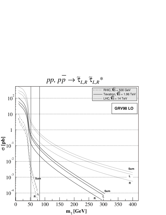
Figure 4.2: Unpolarized hadronic cross sections for non-mixing $\tilde{\tau}$ pair production of at the RHIC, Tevatron, and LHC colliders as a function of $m_{\tilde{\tau}}$. The vertical lines indicate the two different $\tilde{\tau}$ mass limits of 52 [198] and 81.9 GeV [199].

The $\tilde{\tau}$ mass limits imposed by LEP depend strongly on the assumed SUSY-breaking mechanism, the mass difference between the $\tilde{\tau}$ and the LSP, and the mixing angle $\theta_{\tilde{\tau}}$. The weakest limit of 52 GeV is found for GMSB models and stau decays to gravitinos, if no constraints on their mass difference are imposed [198]. This is the scenario that we will study for the RHIC collider, which has the most restricted hadronic centre-of-mass energy, equal to 500 GeV. For the Tevatron and the LHC, with their considerably larger centre-of-mass energies of 1.96 and 14 TeV, respectively, we will, however, impose the stricter mass limit of 81.9 GeV [199], which is valid for staus decaying into neutralinos, with a mass difference of at least 15 GeV.

Thanks to the QCD factorization theorem, the unpolarized hadronic cross section

$$\sigma=\sum_{a,b}\int_{\tau}^{1}{\rm d}x_{a}\int_{\tau/x_{a}}^{1}{\rm d}x_{b}\,f_{a/h_{a}}(x_{a},\mu_{F})\,\ f_{b/h_{b}}(x_{b},\mu_{F})\,\hat{\sigma}_{ab}$$ (4.21)

can be written as the convolution of the relevant partonic cross section $\hat{\sigma}_{ab}$ (integrated here over $t$) with the universal distribution functions $f_{a,b/h_{a,b}}$ of partons $a,b$ inside the hadrons $h_{a,b}$, which depend on the longitudinal momentum fractions of the two partons $x_{a,b}$ and on the unphysical factorization scale $\mu_{F}$. In order to employ a consistent set of unpolarized and polarized parton densities (see next subsection), we choose the LO set of GRV98 [200] for our unpolarized predictions at the factorization scale $\mu_{F}=m_{\tilde{\tau}_{1}}$.

In Fig. 4.2, we show the unpolarized hadronic cross sections for non-mixing $\tilde{\tau}$ pair production at the RHIC, Tevatron, and LHC colliders as a function of the $\tilde{\tau}$ physical mass. The observation of tau sleptons will be difficult at RHIC, which is the only existing polarized hadron collider, but they will be detectable at the Tevatron, extending considerably the discovery reach beyond the current limits. In contrast, at the LHC, $\tilde{\tau}$ pair production will be visible up to masses of 1 TeV. Before application of any experimental cuts, the SUSY signal cross section is at least three orders of magnitude smaller than the corresponding SM background coming from tau lepton pair production. Evaluated using the physical tau mass of $m_{\tau}=1.77699$ GeV as factorization scale for the GRV98 LO parton densities, this cross section is equal to 1.7, 3.4, and 8.3 nb for the RHIC, Tevatron, and LHC colliders, respectively. Imposing an invariant-mass cut on the observed lepton pair and a minimal missing transverse energy will, however, greatly improve the signal-to-background ratio. In addition, as we will see in the next section, asymmetries may provide an important tool to further distinguish the SUSY signal from the corresponding SM process.

4.1.3 Single-spin asymmetries

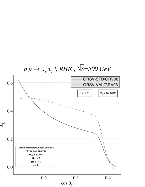
Figure 4.3: Longitudinal single-spin asymmetry $A_{L}$ as a function of the cosine of the stau mixing angle for $\tilde{\tau}_{1}$ pair production at RHIC.

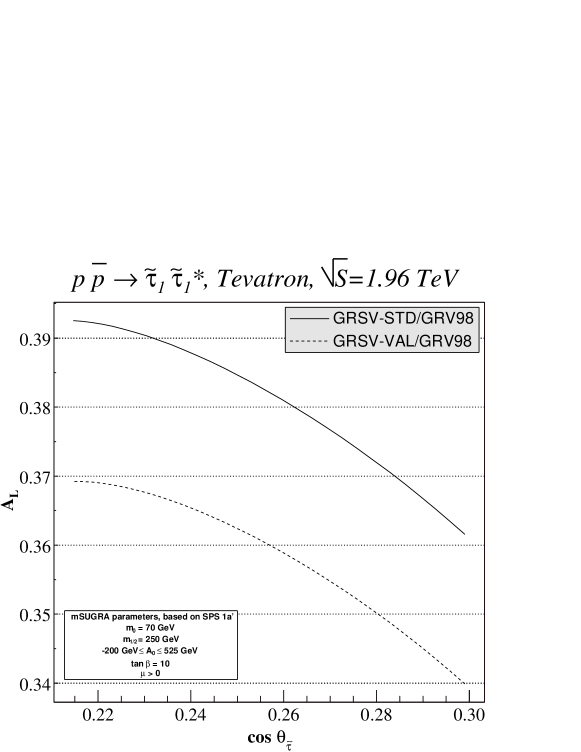
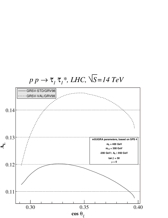
Figure 4.4: Dependence of the longitudinal single-spin asymmetry $A_{L}$ on the cosine of the stau mixing angle for $\tilde{\tau}_{1}$ pair production at the Tevatron (top) and at the LHC (bottom).

Using again the QCD factorization theorem, we calculate the hadronic cross section for longitudinally polarized hadrons $h_{a}$ with unpolarized hadrons $h_{b}$

$$\Delta\sigma_{L}=\sum_{a,b}\int_{\tau}^{1}{\rm d}x_{a}\int_{\tau/x_{a}}^{1}{\rm d}x_{b}\,\Delta f_{a/h_{a}}(x_{a},\mu_{F})\,\ f_{b/h_{b}}(x_{b},\mu_{F})\,{\rm d}\Delta\hat{\sigma}_{L,ab}$$ (4.22)

through a convolution of polarized ($\Delta f_{a/A}$) and unpolarized ($f_{b/B}$) parton densities with the singly polarized partonic cross section $\Delta\hat{\sigma}_{L}$ (integrated over $t$). As mentioned above, we employ a consistent set of unpolarized [200] and polarized [201] LO parton densities. The theoretical uncertainty due to the less well known polarized parton densities is estimated by showing our numerical predictions for both the GRSV2000 LO standard (STD) and valence (VAL) parameterizations.

The physical masses of the SUSY particles and the mixing angles are computed with the program SuSpect 2.3 [202], including a consistent calculation of the Higgs mass, with all one-loop and the dominant two-loop radiative corrections in the renormalization group equations that link the restricted set of SUSY-breaking parameters at the gauge coupling unification scale to the complete set of observable SUSY masses and mixing angles at the electroweak scale. We choose three SPS benchmark points [45, 46], the GMSB point SPS 7 with a light tau slepton decaying to a gravitino for RHIC and its very limited mass range, the typical mSUGRA point SPS 1a’ with an intermediate value of $\tan\beta=10$ and a slightly reduced common scalar mass of $m_{0}=70$ GeV for the Tevatron, and the mSUGRA point SPS 4 with a large scalar mass of $m_{0}=400$ GeV and large $\tan\beta=50$, which enhances mixing, for the LHC with its larger mass range. Since $\theta_{\tilde{\tau}}$ depends directly on the universal soft SUSY-breaking mass scale $\Lambda$ in the GMSB model and on the trilinear coupling $A_{0}$ in the mSUGRA models, we test the sensitivity of the single-spin asymmetry on these parameters (see Figs. 4.3-4.4).

In Fig. 4.3, we show the single-spin asymmetry for $\tilde{\tau}_{1}$ pair production at RHIC as a function of the cosine of the stau mixing angle. The asymmetry is quite large and depends strongly on the stau mixing angle. However, very large values of $\cos\theta_{\tilde{\tau}}$, corresponding to $\tilde{\tau}$ masses below 52 GeV may already be excluded by LEP [198], while small values of $\cos\theta_{\tilde{\tau}}$ may be unaccessible to RHIC limited luminosity, which is not expected to exceed 1 fb^-1. Polarization of the proton beam will also not be perfect, and the calculated asymmetries should be multiplied by the degree of beam polarization $P_{L}\simeq 0.7$. The uncertainty introduced by the polarized parton densities increases considerably to the left of the plot, where the stau mass 41 GeV $\leq m_{\tilde{\tau}}\leq$ 156 GeV and the associated values of the parton momentum fractions $x_{a,b}\simeq 2m_{\tilde{\tau}}/\sqrt{s_{h}}$ become large. While the SM background cross section is then still two orders of magnitude larger than the SUSY signal after imposing an invariant-mass cut on the observed tau lepton pair, the SM asymmetry of -0.04 (-0.10) for STD (VAL) polarized parton densities can clearly be distinguished due to its different sign.

An asymmetry measurement at an upgraded Tevatron would be extremely valuable, since the predicted asymmetry is very sizeable in the entire viable SUSY parameter range, and depends strongly on the parameter $A_{0}$, and then the stau mixing angle (top figure of Fig. 4.4). Unfortunately, the parton density uncertainties are still large, but will be reduced considerably in the future through more precise measurements at the COMPASS, HERMES, PHENIX, and STAR experiments. As a recent experimental study demonstrates, events with tau leptons with associated missing energy larger than 20 GeV can be identified with the CDF-II detector, considering hadronic tau decays [203]. Again, the negative SM asymmetry of -0.09 (for both polarized parton densities) would be clearly distinguishable due to its opposite sign.

For the LHC, where studies of tau slepton identification with the ATLAS detector [204] and tau tagging with the CMS detector [205] have recently been performed, SUSY masses should be observable up to the TeV-range. We show the predicted asymmetry for a possible polarization upgrade of this collider in the bottom panel of Fig. 4.4. It is still comfortably large and has again the opposite sign with respect to the SM asymmetry of -0.02 (for both polarized parton densities). The dependence of the asymmetry on the stau mixing angle is, however, also reduced, while the uncertainties from the polarized parton densities, which are not yet well known at the small $x$ values relevant for the large LHC centre-of-mass energy, are quite enhanced.

4.2 Transverse-momentum spectrum

4.2.1 Analytical results

As said in the introduction, the main SM background to slepton pair production comes from $WW$ and $t\bar{t}$ production. However, an accurate calculation of the transverse-momentum spectrum would allow us to distinguish the signal from the background. A transverse-momentum distribution for slepton pair production at leading order is induced by a final state containing one slepton pair and one QCD jet. The relative partonic cross section can be divided into a resummed and a finite part, as in Eq. (3.64),

$$\frac{{\rm d}{\hat{\sigma}}_{ab}}{{\rm d}M^{2}{\rm d}q_{T}^{2}}=\frac{{\rm d}{\hat{\sigma}}_{ab}^{(\rm res.)}}{{\rm d}M^{2}{\rm d}q_{T}^{2}}+\frac{{\rm d}{\hat{\sigma}}_{ab}^{(\rm fin.)}}{{\rm d}M^{2}{\rm d}q_{T}^{2}},\leavevmode\nobreak\$$ (4.23)

where $a,b$ label the partons which take part in the hard process. In Mellin $N$-space, the (partonic) resummed component is deduced from Eqs. (3.2.4) and (3.2.4),

$$\frac{{\rm d}{\hat{\sigma}}_{ab}^{(\rm res.)}}{{\rm d}M^{2}{\rm d}q_{T}^{2}}(q_{T},M,s;\alpha_{s}(\mu_{R}),\mu_{R},\mu_{F})=\int_{0}^{\infty}{\rm d}b\;\frac{b}{2}\,J_{0}(bq_{T})\,\tilde{W}^{F}_{ab}(N,b;M,\mu_{F},\mu_{R}),$$

(4.24)

$$\tilde{W}^{F}_{ab}(N,b;M,\mu_{F},\mu_{R})\!=\!\mathcal{H}^{F}_{ab}\Big{(}N,\alpha_{s}(\mu_{R});\frac{M}{\mu_{R}},\!\frac{M}{\mu_{F}},\!\frac{M}{Q}\Big{)}\!\exp\!\Big{\{}\mathcal{G}\big{(}N,\tilde{L},\alpha_{s}(\mu_{R});\frac{M}{\mu_{R}},\!\frac{M}{Q}\big{)}\Big{\}},\leavevmode\nobreak\$$

(4.25)

where at the NLL accuracy, the functions ${\cal H}$ and ${\cal G}$ of Eqs. (3.2.4) and (3.2.4) read

$${\cal H}_{ab}^{F}(N,\alpha_{s};\frac{M}{\mu_{R}},\!\frac{M}{\mu_{F}},\!\frac{M}{Q})\!=\!\sum_{c}\sigma_{c\bar{c}}^{({\rm LO})F}(M)\left[\delta_{ac}\delta_{b\bar{c}}\!+\!\left(\frac{\alpha_{s}}{\pi}\right)\,{\cal H}_{ab\to c\bar{c}}^{F(1)}(N;\frac{M}{\mu_{R}},\!\frac{M}{\mu_{F}},\!\frac{M}{Q})\right]\leavevmode\nobreak\ ,$$

(4.26)

$${\cal G}(N,\tilde{L};\alpha_{s},\frac{M}{\mu_{R}},\!\frac{M}{Q})=\tilde{L}\,g^{(1)}(\frac{1}{\pi}\,\beta_{0}\,\alpha_{s}(\mu_{R})\,L)+g^{(2)}(N,\frac{1}{\pi}\,\beta_{0}\,\alpha_{s}(\mu_{R})\,\tilde{L};\frac{M}{\mu_{R}},\!\frac{M}{Q}),\leavevmode\nobreak\$$ (4.27)

with

$${\tilde{L}}=\ln\left(\frac{Q^{2}\,b^{2}}{b_{0}^{2}}+1\right),\leavevmode\nobreak\$$ (4.28)

this definition of $\tilde{L}$ allowing us to avoid the unwanted resummed contributions in the small-$b$ region. The explicit expression of $g^{(1)}$ and $g^{(2)}$ in terms of the universal perturbative coefficients $A^{(1)}_{q}$, $A^{(2)}_{q}$, and $B^{(1)}_{q}$ (see Eqs. (3.25), (3.26) and 3.27)) are given by Eqs. (3.55) and (3.56). Slepton pair production being similar to SM lepton pair production, except for the final state, we can use the Drell-Yan coefficients ${\cal H}^{(1)}$ from Eqs. (3.51) and (3.52), but the Born cross section $\sigma^{({\rm LO})F}(M)$ in Eq. (4.2.1) corresponds obviously to the slepton pair production one, which can be obtained for neutral and charged currents by integrating Eqs. (4.12) and (4.13) over $t$, respectively,

$$\sigma_{q\bar{q}}^{(LO)}(M) = \frac{\alpha^{2}\,\pi\,\beta^{3}}{9\,M^{2}}\Bigg{[}e_{q}^{2}\,e_{l}^{2}\,\delta_{ij}+\frac{e_{q}\,e_{l}\,\delta_{ij}(L_{qqZ}+R_{qqZ})\,{\rm Re}\left[L_{\tilde{l}_{i}\tilde{l}_{j}Z}+R_{\tilde{l}_{i}\tilde{l}_{j}Z}\right]}{4\,x_{W}\,(1-x_{W})\,(1-m_{Z}^{2}/M^{2})}$$ (4.29)

$$+ \,\frac{(L_{qqZ}^{2}+R_{qqZ}^{2})\left|L_{\tilde{l}_{i}\tilde{l}_{j}Z}+R_{\tilde{l}_{i}\tilde{l}_{j}Z}\right|^{2}}{32\,x_{W}^{2}\,(1-x_{W})^{2}(1-m_{Z}^{2}/M^{2})^{2}}\Bigg{]},\leavevmode\nobreak\$$

$$\sigma_{q\bar{q}^{\prime}}^{(LO)}(M) = \frac{\alpha^{2}\,\pi\,\beta^{3}}{9\,M^{2}}\Bigg{[}\frac{\left|L_{qq^{\prime}W}L_{\tilde{l}_{i}\tilde{\nu}_{l}W}\right|^{2}}{32\,x_{W}^{2}\,(1-x_{W})^{2}(1-m_{W}^{2}/M^{2})^{2}}\Bigg{]},\leavevmode\nobreak\$$ (4.30)

where the slepton-mass dependence is factorized in the velocity

$$\beta = \sqrt{1+m_{i}^{4}/M^{4}+m_{j}^{4}/M^{4}-2(m_{i}^{2}/M^{2}+m_{j}^{2}/M^{2}+m_{i}^{2}\,m_{j}^{2}/M^{4})},\leavevmode\nobreak\$$ (4.31)

$m_{i}$ and $m_{j}$ being the two masses of the final state particles.

The second term (${\rm d}{\hat{\sigma}}_{ab}^{(\rm fin.)}/{\rm d}M^{2}{\rm d}q_{T}^{2}$) in Eq. (4.23) is free of divergent contributions and can be computed by fixed-order truncation of the perturbative series, as in Eq. (3.62). In order to be consistently matched with the resummed contribution at intermediate $q_{T}$ ($q_{T}\simeq M$), this term is evaluated starting from the usual perturbative calculation of the partonic cross section from which we subtract the expansion of the resummed component of the cross section at the same perturbative order. In order to consistently perform a NLL+LO matching, we need the fixed-order cross section relative to the production of a slepton pair with non-vanishing transverse-momentum at order $\alpha_{s}$, i.e. one slepton pair plus one parton [39, 40]. The different channels read

$${{\rm d}{\hat{\sigma}}_{qg}\over{\rm d}M^{2}{\rm d}q_{T}^{2}} = \frac{\alpha_{s}(\mu_{R})\,T_{R}}{2\,\pi\,s}A_{qg}(s,t,u;M^{2})\,\sigma_{q\bar{q}^{(\prime)}}^{(LO)}(M),\leavevmode\nobreak\$$ (4.32)

$${{\rm d}{\hat{\sigma}}_{g\bar{q}}\over{\rm d}M^{2}{\rm d}q_{T}^{2}} = \frac{\alpha_{s}(\mu_{R})\,T_{R}}{2\,\pi\,s}A_{qg}(s,u,t;M^{2})\,\sigma_{q\bar{q}^{(\prime)}}^{(LO)}(M),\leavevmode\nobreak\$$ (4.33)

$${{\rm d}{\hat{\sigma}}_{q\bar{q}^{(\prime)}}\over{\rm d}M^{2}{\rm d}q_{T}^{2}} = \frac{\alpha_{s}(\mu_{R})\,C_{F}}{2\,\pi\,s}A_{qq}(s,t,u;M^{2})\,\sigma_{q\bar{q}^{(\prime)}}^{(LO)}(M),\leavevmode\nobreak\$$ (4.34)

where $s$, $t$, and $u$ denote the partonic Mandelstam variables relative to the $2\to 2$ subprocess $ab\to\gamma,Z^{0},W^{\mp}+{\rm one\leavevmode\nobreak\ parton}$,

$$s = x_{a}x_{b}s_{h},$$ (4.35)

$$t = M^{2}-\sqrt{s_{h}(M^{2}+q^{2}_{T})}x_{b}e^{y},$$ (4.36)

$$u = M^{2}-\sqrt{s_{h}(M^{2}+q^{2}_{T})}x_{a}e^{-y},$$ (4.37)

$y$ being the rapidity of the slepton pair. We have defined the $A_{ab}$-functions as [206],

$$A_{qg}(s,t,u;M^{2}) = -\left(\frac{s}{t}+\frac{t}{s}+\frac{2u\,M^{2}}{st}\right),\leavevmode\nobreak\$$ (4.38)

$$A_{qq}(s,t,u;M^{2}) = -A_{qg}(u,t,s;M^{2}).\leavevmode\nobreak\$$ (4.39)

It is known [57] that the transverse-momentum distribution is affected by non-perturbative effects which become important in the large-$b$ region. In the case of electroweak boson production, these contributions are usually parameterized by multiplying the function $\tilde{W}^{F}$ in Eq. (4.2.1) by a NP form factor $F^{NP}(b)$ [172, 176, 177, 178, 179], whose coefficients are obtained through global fits to DY data. We include in our analysis three different parameterizations of non-perturbative effects corresponding to three different choices of the form factor: the Ladinsky-Yuan (LY-G) [176], Brock-Landry-Nadolsky-Yuan (BLNY) [178], and the recent Konychev-Nadolsky (KN) [179] form factor. The explicit expressions can be found in Eqs. (3.32), (3.33) and (3.34).

4.2.2 Numerical results

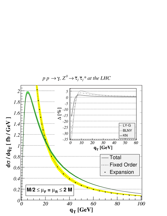
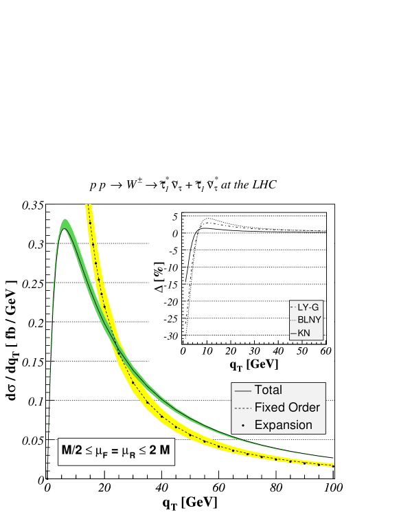
Figure 4.5: Differential cross section for the processes $pp\to\tilde{\tau}_{1}\tilde{\tau}_{1}^{\ast}$ (top) and $pp\to\tilde{\tau}_{1}\tilde{\nu}_{\tau}^{\ast}+\tilde{\tau}_{1}^{\ast}\tilde{\nu}_{\tau}$ (bottom). NLL+LO matched result, LO result, asymptotic expansion of the resummation formula and $\Delta$-parameter are shown.

We present quantitative results for the $q_{T}$-spectrum of slepton pair (slepton-sneutrino associated) production at NLL+LO accuracy at the LHC collider. For the masses and widths of the electroweak gauge bosons, the electroweak mixing angle and the electromagnetic fine structure constant, we use the same values as those given in Sec. 4.1.2, while the CKM-matrix elements are computed as in Sec. 2.3.3. As in the previous section, we focus our study on the lightest slepton mass eigenstate ${\tilde{\tau}}_{1}$ and thus we consider the processes

$$\begin{array}[]{c}q\bar{q}\to\gamma,Z^{0}\to\tilde{\tau}_{1}\tilde{\tau}^{\ast}_{1},\\ q\bar{q}^{\prime}\to W^{\mp}\to\tilde{\tau}_{1}\tilde{\nu}_{\tau}^{\ast},\tilde{\tau}^{*}_{1}\tilde{\nu}_{\tau}.\end{array}$$ (4.42)

We use the MRST (2004) NLO set of parton distribution functions [207] and $\alpha_{s}$ is evaluated at two-loop accuracy. We fix the resummation scale $Q$ (see Eq. (3.2.4)) equal to the invariant-mass $M$ of the slepton (slepton-sneutrino) pair and we allow $\mu=\mu_{F}=\mu_{R}$ to vary between $M/2$ and $2M$ to estimate the perturbative uncertainty. We also integrate Eq. (4.23) with respect to $M^{2}$, taking as lower limit the energy threshold for $\tilde{\tau}_{1}\tilde{\tau}_{1}^{\ast}$ $(\tilde{\tau}_{1}\tilde{\nu}_{\tau})$ production and as upper limit the hadronic energy ($\sqrt{s}_{h}$ = 14 TeV at the LHC).

In the case of $\tilde{\tau}_{1}\tilde{\tau}_{1}^{*}$ production (neutral current process, see the top panel of Fig. 4.5), we choose the SPS 7 GMSB benchmark point [45] which gives, after the renormalization group evolution of the SUSY-breaking parameters performed by the SuSpect computer program [202], a light ${\tilde{\tau}}_{1}$ of mass $m_{{\tilde{\tau}}_{1}}=114$ GeV. In the case of $\tilde{\tau}_{1}\tilde{\nu}_{\tau}^{\ast}+\tilde{\tau}_{1}^{\ast}\tilde{\nu}_{\tau}$ production (charged current process, see the bottom panel of Fig. 4.5), we use instead the SPS 1a mSUGRA benchmark point which gives a light ${\tilde{\tau}}_{1}$ of mass $m_{{\tilde{\tau}}_{1}}=136$ GeV as well as a light $\tilde{\nu}_{\tau}$ of mass $m_{{\tilde{\nu}}_{\tau}}=196$ GeV.

In both cases we plot the LO result (dashed line) and the total NLL+LO matched result (solid line) with their uncertainty band relative to scale variation (yellow band for LO result, and green band for NLL+LO result). The expansion of the resummation formula at LO (dotted line) is also shown. We can see that the LO result diverges, as expected from the generic form of the fixed-order cross section in Eq. (3.18), for both processes as $q_{T}\to 0$. The asymptotic expansion of the resummation formula at LO is in very good agreement with LO both at small and intermediate values of $q_{T}$, from which we can conclude that the cross section is clearly dominated by the logarithms that we are resumming in this kinematical region. The effect of resummation is clearly visible at small and intermediate values of $q_{T}$, the resummation-improved result being nearly 39% (36%) higher at $q_{T}=50$ GeV than the pure fixed-order result in the neutral (charged) current case. When integrated over $q_{T}$, the former leads to a total cross section of 66.8 fb (12.9 fb) in good agreement (within 3.5%) with the QCD-corrected total cross section at ${\cal O}(\alpha_{s})$ [40].

The scale dependence is clearly improved in both cases with respect to the pure fixed-order calculations. In the small and intermediate $q_{T}$-region (up to 100 GeV) the effect of scale variation is 10% for the LO result, while it is always less than 5% for the NLL+LO curve.

Finally, we study the dependence of the total NLL+LO matched result on non-perturbative effects. We show the quantity $\Delta$

$$\Delta=\frac{d\sigma^{\rm(res.+NP)}(\mu=M)-d\sigma^{(\rm res.)}(\mu=M)}{d\sigma^{(\rm res.)}(\mu=M)},$$ (4.43)

as a function of the transverse momentum of the slepton pair. The parameter $\Delta$ gives thus an estimate of the contributions from the different NP parameterizations (LY-G, BLNY, KN) that we included in the resummed formula, which are under good control, since they are always less than 5% for $q_{T}>$ 5 GeV and thus considerably smaller than the resummation effects.

4.3 Invariant-mass distributions

4.3.1 Next-to-leading order calculations

Restoring the various scale dependences in the QCD factorization theorem of Eq. (4.21), the invariant-mass distribution of a given process can be written as

$$\sigma=\sum_{a,b}\int_{\tau}^{1}{\rm d}x_{a}\int_{\tau/x_{a}}^{1}{\rm d}x_{b}\,f_{a/h_{a}}(x_{a},\mu_{F})\,\ f_{b/h_{b}}(x_{b},\mu_{F})\,\hat{\sigma}_{ab}\left(z,M;\alpha_{s}(\mu_{R}),\frac{M}{\mu_{F}},\frac{M}{\mu_{R}}\right),\leavevmode\nobreak\$$

(4.44)

where $M$ is the invariant-mass. The partonic cross section is usually expanded in powers of $\alpha_{s}$

$$\hat{\sigma}_{ab}\left(z,M;\alpha_{s}(\mu_{R}),\frac{M}{\mu_{F}},\frac{M}{\mu_{R}}\right) = \sum_{n=0}^{\infty}\left(\frac{\alpha_{s}(\mu_{R})}{\pi}\right)^{n}\sigma_{ab}^{(n)}\left(z,M;\frac{M}{\mu_{F}},\frac{M}{\mu_{R}}\right).\leavevmode\nobreak\$$ (4.45)

Concerning slepton pair hadroproduction, we have computed the LO ($n=0$) coefficients in the previous sections, which read, showing explicitly the dependence on the scaling variable $z=M^{2}/s$,

$$\sigma_{q\bar{q}^{(\prime)}}^{(0)}\left(z,M;\frac{M}{\mu_{F}},\frac{M}{\mu_{R}}\right) = \sigma_{0}^{(\prime)}(M)\,\delta(1-z),\leavevmode\nobreak\$$ (4.46)

$\sigma_{0}$ and $\sigma_{0}^{\prime}$ being defined in Eqs. (4.29) and (4.30) for the neutral and charged currents, respectively,

$$\sigma_{0}(M) = \frac{\alpha^{2}\,\pi\,\beta^{3}}{9\,M^{2}}\Bigg{[}e_{q}^{2}\,e_{l}^{2}\,\delta_{ij}+\frac{e_{q}\,e_{l}\,\delta_{ij}(L_{qqZ}+R_{qqZ})\,{\rm Re}\left[L_{\tilde{l}_{i}\tilde{l}_{j}Z}+R_{\tilde{l}_{i}\tilde{l}_{j}Z}\right]}{4\,x_{W}\,(1-x_{W})\,(1-m_{Z}^{2}/M^{2})}$$ (4.47)

$$+ \,\frac{(L_{qqZ}^{2}+R_{qqZ}^{2})\left|L_{\tilde{l}_{i}\tilde{l}_{j}Z}+R_{\tilde{l}_{i}\tilde{l}_{j}Z}\right|^{2}}{32\,x_{W}^{2}\,(1-x_{W})^{2}(1-m_{Z}^{2}/M^{2})^{2}}\Bigg{]},\leavevmode\nobreak\$$

$$\sigma_{0}^{\prime}(M) = \frac{\alpha^{2}\,\pi\,\beta^{3}}{9\,M^{2}}\Bigg{[}\frac{\left|L_{qq^{\prime}W}L_{\tilde{l}_{i}\tilde{\nu}_{l}W}\right|^{2}}{32\,x_{W}^{2}\,(1-x_{W})^{2}(1-m_{W}^{2}/M^{2})^{2}}\Bigg{]}.\leavevmode\nobreak\$$ (4.48)

The NLO QCD and SUSY-QCD corrections, i.e. the $n=1$-coefficients in the perturbative expansion of Eq. (4.45), have been studied for non-mixing sleptons in [39, 40]. At NLO, the quark-antiquark annihilation process receives contributions from virtual gluon exchange (see upper part of Fig. 4.8), real gluon emission (see Fig. 4.8) diagrams, and we also have to take into account the quark-gluon initiated subprocesses (see Fig. 4.8).

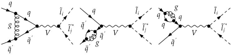
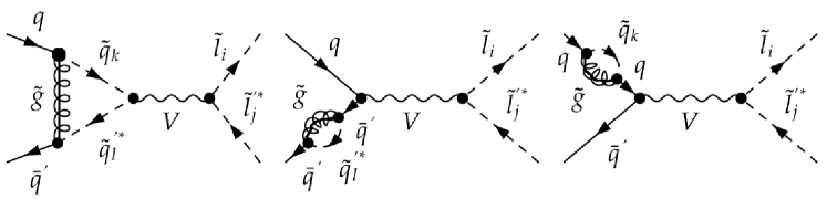
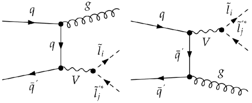
Figure 4.6: Contributions of virtual diagrams for slepton pair ($V=\gamma,Z^{0}$) and slepton-sneutrino associated ($V=W^{\mp}$) production at next-to-leading order in perturbative QCD. The first and second lines show the QCD and SUSY-QCD corrections, respectively. In the SUSY-QCD case, one has to sum over squark mass-eigenstates $k,l=1,2$.

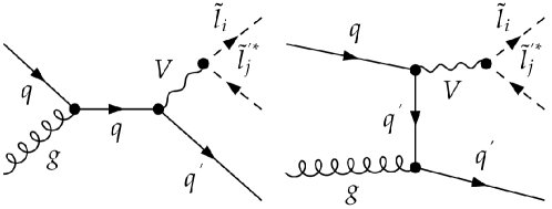
Figure 4.7: Contributions from real gluon emission diagrams for slepton pair ($V=\gamma,Z^{0}$) and slepton-sneutrino associated ($V=W^{\mp}$) production at next-to-leading order in perturbative QCD.

Figure 4.8: Contributions from $qg$ diagrams for slepton pair ($V=\gamma,Z^{0}$) and slepton-sneutrino associated ($V=W^{\mp}$) production at next-to-leading order in perturbative QCD.

The infrared and collinear singularities of the three-parton cross sections are extracted using the dipole subtraction formalism [208], and the virtual corrections have been evaluated in the $\overline{{\rm MS}}$ renormalization scheme. For the SM QCD diagrams one has the well-known results [39, 209]

$$\sigma_{q\bar{q}^{(\prime)}}^{(1;{\rm QCD})}\left(z,M;\frac{M}{\mu_{F}},\frac{M}{\mu_{R}}\right) = \sigma_{0}^{(\prime)}(M)\,C_{F}\,\Bigg{[}\left(\frac{\pi^{2}}{3}-4\right)\,\delta(1-z)+4\left(\frac{\ln(1-z)}{1-z}\right)_{+}$$ (4.49)

$$\!-\! \frac{1+z^{2}}{1-z}\,\ln z\!-\!2\,(1+z)\ln(1-z)\!+\!\frac{2P_{qq}^{(0)}(z)}{C_{F}}\,\ln{\frac{M^{2}}{\mu_{F}^{2}}}\Bigg{]},\leavevmode\nobreak\$$

$$\sigma_{qg}^{(1;{\rm QCD})}\left(z,M;\frac{M}{\mu_{F}},\frac{M}{\mu_{R}}\right) = \sigma_{0}^{(\prime)}(M)\,T_{R}\,\Bigg{[}\left(\frac{1}{2}-z+z^{2}\right)\ln\frac{(1-z)^{2}}{z}+\frac{1}{4}+\frac{3z}{2}$$ (4.50)

$$- \frac{7z^{2}}{4}+\frac{P_{qg}^{(0)}(z)}{T_{R}}\ln\frac{M^{2}}{\mu_{F}^{2}}\Bigg{]},\leavevmode\nobreak\$$

which expose the LO cross-sections $\sigma_{0}^{(\prime)}(M)$ in factorized form. $C_{F}=4/3$ and $T_{R}=1/2$ are the usual QCD colour factors, and $P_{qq,qg}^{(0)}$ are the Altarelli-Parisi splitting functions [210]

$$P_{qq}^{(0)}(z) = \frac{C_{F}}{2}\left[\frac{3}{2}\,\delta(1-z)+\frac{2}{(1-z)_{+}}-(1+z)\right]\leavevmode\nobreak\ \leavevmode\nobreak\ {\rm and}$$ (4.51)

$$P_{qg}^{(0)}(z) = \frac{T_{R}}{2}\left[z^{2}+(1-z)^{2}\right].$$ (4.52)

We remind the reader that our normalization corresponds to a perturbative expansion in powers of $\alpha_{s}/\pi$.

The three lower diagrams of Fig. 4.8 contain SUSY-QCD corrections. We generalize the results from [40] to the case of mixed squark mass eigenstates $k,l=1,2$ in the virtual loop diagrams, obtaining for neutral and charged currents [73]

$$\sigma_{q\bar{q}}^{(1;{\rm SUSY})}\left(z,M;\frac{M}{\mu_{F}},\frac{M}{\mu_{R}}\right) = \frac{\alpha^{2}\,\pi\,\beta^{3}\,C_{F}}{36\,M^{2}}\Bigg{[}f_{\gamma}\,e_{q}^{2}\,e_{l}^{2}\,\delta_{ij}$$ (4.53)

$$+ f_{\gamma Z}\,\frac{e_{q}\,e_{l}\,\delta_{ij}{\rm Re}\left[L_{Z\tilde{l}_{i}\tilde{l}_{j}}+R_{Z\tilde{l}_{i}\tilde{l}_{j}}\right]}{4\,x_{W}\,(1-x_{W})\,(1-m_{Z}^{2}/M^{2})}$$

$$+ f_{Z}\,\frac{\left|L_{Z\tilde{l}_{i}\tilde{l}_{j}}\!+\!R_{Z\tilde{l}_{i}\tilde{l}_{j}}\right|^{2}}{32\,x_{W}^{2}\,(1\!-\!x_{W})^{2}(1\!-\!m_{Z}^{2}/M^{2})^{2}}\Bigg{]}\,\delta(1\!-\!z),\leavevmode\nobreak\$$

$$\sigma_{q\bar{q}^{\prime}}^{(1;{\rm SUSY})}\left(z,M;\frac{M}{\mu_{F}},\frac{M}{\mu_{R}}\right) = \frac{\alpha^{2}\,\pi\,\beta^{3}\,C_{F}}{36\,M^{2}}\Bigg{[}\frac{f_{W}\,\left|L_{W\tilde{l}_{i}\tilde{\nu}_{l}}\right|^{2}\,\delta(1\!-\!z)}{32\,x_{W}^{2}(1\!-\!x_{W})^{2}(1\!-\!m_{W}^{2}/M^{2})^{2}}\Bigg{]},\leavevmode\nobreak\ \leavevmode\nobreak\ \leavevmode\nobreak\ \leavevmode\nobreak\ \leavevmode\nobreak\ \leavevmode\nobreak\ \leavevmode\nobreak\$$ (4.54)

where now only the diagonal squared photon contribution to the Born cross section factorizes. The virtual loop coefficients $f_{\gamma}$, $f_{\gamma Z}$, $f_{Z}$ and $f_{W}$ are

$$f_{\gamma} = 2+\sum_{i=1,2}\Bigg{[}\frac{2\,m_{\tilde{g}}^{2}-2\,m_{\tilde{q}_{i}}^{2}+M^{2}}{M^{2}}\,\Big{(}B_{0f}\left(M^{2},m_{\tilde{q}_{i}}^{2},m_{\tilde{q}_{i}}^{2}\right)-B_{0f}\left(0,m_{\tilde{g}}^{2},m_{\tilde{q}_{i}}^{2}\right)\Big{)}$$ (4.55)

$$+ \left(m_{\tilde{q}_{i}}^{2}-m_{\tilde{g}}^{2}\right)\,B^{\prime}_{0f}\left(0,m_{\tilde{g}}^{2},m_{\tilde{q}_{i}}^{2}\right)$$

$$+ 2\,\frac{m_{\tilde{g}}^{4}+(M^{2}-2\,m_{\tilde{q}_{i}}^{2})\,m_{\tilde{g}}^{2}+m_{\tilde{q}_{i}}^{4}}{M^{2}}C_{0f}\left(0,M^{2},0,m_{\tilde{q}_{i}}^{2},m_{\tilde{g}}^{2},m_{\tilde{q}_{i}}^{2}\right)\Bigg{]},\leavevmode\nobreak\$$

$$f_{\gamma Z} = 2\,(L_{Zqq}+R_{Zqq})$$ (4.56)

$$+ \sum_{i=1,2}\Bigg{[}2\,\frac{\left(2\,m_{\tilde{g}}^{2}-2\,m_{\tilde{q}_{i}}^{2}+M^{2}\right)\,{\rm Re}\Big{[}L_{Z\tilde{q}_{i}\tilde{q}_{i}}+R_{Z\tilde{q}_{i}\tilde{q}_{i}}\Big{]}}{M^{2}}\,B_{0f}\left(M^{2},m_{\tilde{q}_{i}}^{2},m_{\tilde{q}_{i}}^{2}\right)\Bigg{]}$$

$$- \sum_{i=1,2}\!\Bigg{[}2\,\frac{\left(2\,m_{\tilde{g}}^{2}\!-\!2\,m_{\tilde{q}_{i}}^{2}\!+\!M^{2}\right)\,\Big{(}L_{Zqq}\,\Big{|}S^{\tilde{q}}_{i1}\Big{|}^{2}\!+\!R_{Zqq}\,\Big{|}S^{\tilde{q}}_{i1}\Big{|}^{2}\Big{)}}{M^{2}}\,B_{0f}\left(0,m_{\tilde{g}}^{2},m_{\tilde{q}_{i}}^{2}\right)\Bigg{]}$$

$$+ \sum_{i=1,2}\Bigg{[}\left(m_{\tilde{q}_{i}}^{2}-m_{\tilde{g}}^{2}\right)(L_{Zqq}+R_{Zqq})\,B_{0f}^{\prime}\left(0,m_{\tilde{g}}^{2},m_{\tilde{q}_{i}}^{2}\right)\Bigg{]}$$

$$+ \sum_{i=1,2}\Bigg{[}4\,\frac{\left(m_{\tilde{g}}^{4}+(M^{2}-2\,m_{\tilde{q}_{i}}^{2})\,m_{\tilde{g}}^{2}+m_{\tilde{q}_{i}}^{4}\right)\,{\rm Re}\Big{[}L_{Z\tilde{q}_{i}\tilde{q}_{i}}+R_{Z\tilde{q}_{i}\tilde{q}_{i}}\Big{]}}{M^{2}}$$

$$\hskip 34.1433pt\times C_{0f}\left(0,M^{2},0,m_{\tilde{q}_{i}}^{2},m_{\tilde{g}}^{2},m_{\tilde{q}_{i}}^{2}\right)\Bigg{]},\leavevmode\nobreak\$$

$$f_{Z} = 2\,\left(L_{Zqq}^{2}+R_{Zqq}^{2}\right)$$

$$+ \sum_{i,j=1,2}\left[2\,\frac{\left(2\,m_{\tilde{g}}^{2}\!-\!m_{\tilde{q}_{i}}^{2}\!-\!m_{\tilde{q}_{j}}^{2}\!+\!M^{2}\right)}{M^{2}}\,\Big{|}L_{Z\tilde{q}_{i}\tilde{q}_{j}}\!+\!R_{Z\tilde{q}_{i}\tilde{q}_{j}}\Big{|}^{2}\,B_{0f}\left(M^{2},m_{\tilde{q}_{i}}^{2},m_{\tilde{q}_{j}}^{2}\right)\right]$$

$$- \!\sum_{i=1,2}\Bigg{[}2\,\frac{\left(2\,m_{\tilde{g}}^{2}\!-\!2\,m_{\tilde{q}_{i}}^{2}\!+\!M^{2}\right)\,\Big{(}L^{2}_{Zqq}\,\Big{|}S^{\tilde{q}}_{i1}\Big{|}^{2}\!+\!R^{2}_{Zqq}\,\Big{|}S^{\tilde{q}}_{i2}\Big{|}^{2}\Big{)}}{M^{2}}\,B_{0f}\left(0,m_{\tilde{g}}^{2},m_{\tilde{q}_{i}}^{2}\right)\Bigg{]}$$ (4.57)

$$+ \!\sum_{i=1,2}\Bigg{[}\left(m_{\tilde{q}_{i}}^{2}-m_{\tilde{g}}^{2}\right)\left(L_{Zqq}^{2}+R_{Zqq}^{2}\right)\,B_{0f}^{\prime}\left(0,m_{\tilde{g}}^{2},m_{\tilde{q}_{i}}^{2}\right)\Bigg{]}$$

$$+ \!\sum_{i,j=1,2}\Bigg{[}4\,\frac{\left(m_{\tilde{g}}^{4}+\left(M^{2}-m_{\tilde{q}_{i}}^{2}-m_{\tilde{q}_{j}}^{2}\right)\,m_{\tilde{g}}^{2}+m_{\tilde{q}_{i}}^{2}\,m_{\tilde{q}_{j}}^{2}\right)}{M^{2}}\,\Big{|}L_{Z\tilde{q}_{i}\tilde{q}_{j}}+R_{Z\tilde{q}_{i}\tilde{q}_{j}}\Big{|}^{2}$$

$$\hskip 34.1433pt\times C_{0f}\left(0,M^{2},0,m_{\tilde{q}_{i}}^{2},m_{\tilde{g}}^{2},m_{\tilde{q}_{j}}^{2}\right)\Bigg{]},\leavevmode\nobreak\$$

$$f_{W} = 2\,\Big{|}L_{Wqq^{\prime}}\Big{|}^{2}$$ (4.58)

$$+ \!\sum_{i,j=1,2}\Bigg{[}\frac{2\left(2\,m_{\tilde{g}}^{2}\!-\!m_{\tilde{q}_{i}}^{2}\!-\!m_{\tilde{q}^{\prime}_{j}}^{2}\!+\!M^{2}\right)\Big{|}L_{W\tilde{q}_{i}\tilde{q}_{j}^{\prime}}\Big{|}^{2}}{M^{2}}\,B_{0f}\left(M^{2},m_{\tilde{q}_{i}}^{2},m_{\tilde{q}^{\prime}_{j}}^{2}\right)\!\Bigg{]}$$

$$- \!\sum_{\tilde{Q}=\tilde{q},\tilde{q}^{\prime}}\!\sum_{i=1,2}\Bigg{[}\frac{\left(2\,m_{\tilde{g}}^{2}\!-\!2\,m_{\tilde{Q}_{i}}^{2}\!+\!M^{2}\right)B_{0f}\left(0,m_{\tilde{g}}^{2},m_{\tilde{Q}_{i}}^{2}\right)\Big{|}L_{Wqq^{\prime}}\,S^{\tilde{Q}}_{i1}\,\Big{|}^{2}}{M^{2}}\Bigg{]}$$

$$+ \!\sum_{\tilde{Q}=\tilde{q},\tilde{q}^{\prime}}\,\sum_{i=1,2}\Bigg{[}\frac{1}{2}\left(m_{\tilde{Q}_{i}}^{2}-m_{\tilde{g}}^{2}\right)\,\Big{|}L_{Wqq^{\prime}}\Big{|}^{2}\,B_{0f}^{\prime}\left(0,m_{\tilde{g}}^{2},m_{\tilde{Q}_{i}}^{2}\right)\Bigg{]}$$

$$+ \!\sum_{i,j=1,2}\Bigg{[}\frac{4\left(m_{\tilde{g}}^{4}-\left(m_{\tilde{q}_{i}}^{2}+m_{\tilde{q}^{\prime}_{j}}^{2}-M^{2}\right)\,m_{\tilde{g}}^{2}+m_{\tilde{q}_{i}}^{2}\,m_{\tilde{q}^{\prime}_{j}}^{2}\right)\Big{|}L_{W\tilde{q}_{i}\tilde{q}_{j}^{\prime}}\Big{|}^{2}}{M^{2}}$$

$$\hskip 34.1433pt\times C_{0f}\left(0,M^{2},0,m_{\tilde{q}^{\prime}_{i}}^{2},m_{\tilde{g}}^{2},m_{\tilde{q}_{j}}^{2}\right)\Bigg{]}.\leavevmode\nobreak\$$

The functions $B_{0f}(p^{2},m_{1}^{2},m_{2}^{2})$, $B_{0f}^{\prime}(p^{2},m_{1}^{2},m_{2}^{2})$ and $C_{0f}(p_{1}^{2},(p_{1}+p_{2})^{2},p_{2}^{2},m_{1}^{2},m_{2}^{2},m_{3}^{2})$ are the finite parts of the scalar two- and three-point functions

$$B_{0}(p^{2},m_{1}^{2},m_{2}^{2}) = \mu_{R}^{2\varepsilon}\,\int\frac{{\rm d}^{D}q}{i\pi^{2}}\,\frac{1}{q^{2}\!-\!m_{1}^{2}}\frac{1}{(q\!+\!p)^{2}\!-\!m_{2}^{2}},\leavevmode\nobreak\$$ (4.59)

$$B_{0}^{\prime}(p^{2},m_{1}^{2},m_{2}^{2}) = \frac{{\rm d}B_{0}(k^{2},m_{1}^{2},m_{2}^{2})}{{\rm d}k^{2}}\Big{|}_{k^{2}=p^{2}},\leavevmode\nobreak\$$ (4.60)

$$C_{0}(p_{1}^{2},(p_{1}+p_{2})^{2},p_{2}^{2},m_{1}^{2},m_{2}^{2},m_{3}^{2}) = \mu_{R}^{2\varepsilon}\,\int\frac{{\rm d}^{D}q}{i\pi^{2}}\,\frac{1}{q^{2}-m_{1}^{2}}\frac{1}{(q+p_{1})^{2}-m_{2}^{2}}$$ (4.61)

$$\times\frac{1}{(q+p_{1}+p_{2})^{2}-m_{3}^{2}}.$$

Our results agree with those of Ref. [211] in the case of mass-degenerate non-mixing squarks. Note that the quark mass, which appears in the off-diagonal mass matrix elements of the squarks running in the loops (see Eq. (2.38)), corresponds to a linear Yukawa coupling in the superpotential and can not be neglected, even if it is much smaller than the total centre-of-mass energy of the colliding partons allowing for a massless factorization inside the outer hadrons. The full NLO contributions to the cross section are then given by

$$\sigma_{q\bar{q}^{(\prime)}}^{(1)}\!\left(z,M;\frac{M}{\mu_{F}},\frac{M}{\mu_{R}}\right)\!\!=\!\sigma_{q\bar{q}^{(\prime)}}^{(1;{\rm QCD})}\left(z,M;\frac{M}{\mu_{F}},\frac{M}{\mu_{R}}\right)\!+\!\sigma_{q\bar{q}^{(\prime)}}^{(1;{\rm SUSY})}\left(z,M;\frac{M}{\mu_{F}},\frac{M}{\mu_{R}}\right),\leavevmode\nobreak\ \leavevmode\nobreak\ \leavevmode\nobreak\ \leavevmode\nobreak\$$ (4.62)

$$\sigma_{qg}^{(1)}\left(z,M;\frac{M}{\mu_{F}},\frac{M}{\mu_{R}}\right)=\sigma_{qg}^{(1;{\rm QCD})}\left(z,M;\frac{M}{\mu_{F}},\frac{M}{\mu_{R}}\right).\leavevmode\nobreak\$$ (4.63)

4.3.2 Threshold-enhanced contributions

Eqs. (4.49) and (4.50) explicitly show logarithmic terms of the form $\alpha_{s}[\ln(1-z)/(1-z)]_{+}$. When the initial partons have just enough energy to produce the slepton pair in the final state, i.e. $z$ is close to one, these terms can become large and have to be resummed to all order in $\alpha_{s}$ in order to correctly quantify the effect of this set of corrections, corresponding to soft-collinear gluon emission. Collinear parton-emission can also be taken into account, using the collinear-improved resummation formalism which is described in Sec. 3.3 for Drell-Yan pair production, which can directly be applied to slepton pair production by replacing the Born cross sections by those of Eqs. (4.47) and (4.48). In Mellin space, we have then

$$\hat{\sigma}^{({\rm res})}_{ab}(N,\alpha_{s})=\sigma_{0}^{(\prime)}\,\tilde{C}_{ab}(\alpha_{s})\,\exp\Big{[}S(N,\alpha_{s})\Big{]},\leavevmode\nobreak\$$ (4.64)

with

$$\tilde{C}^{(1)}_{q\bar{q}} = C_{F}\left(\frac{2\,\pi^{2}}{3}-4+\frac{3}{2}\ln\frac{M^{2}}{\mu^{2}_{F}}\right)+2\,A^{(1)}\,\frac{\ln{\bar{N}}-\frac{1}{2}\ln{\frac{M^{2}}{\mu_{F}^{2}}}}{N}\leavevmode\nobreak\ ,$$ (4.65)

$$\tilde{C}^{(1)}_{qg} = -T_{R}\,\frac{\ln{\bar{N}}-\frac{1}{2}\ln{\frac{M^{2}}{\mu_{F}^{2}}}}{N},\leavevmode\nobreak\$$ (4.66)

the Sudakov form factor $S$ being defined by Eqs. (3.79), (3.80) and (3.81). The errors due to missing high-order corrections can be estimated by comparing our results with those obtained by taking the resummed contribution given by Eq. (3.85), where the hard contributions exponentiate as well,

$$\hat{\sigma}^{({\rm res})}_{ab}(N,\alpha_{s})=\sigma^{(LO)}\,\exp\Big{[}C^{(1)}_{q\bar{q}}(\alpha_{s})\Big{]}\,\exp\Big{[}S(N,\alpha_{s})\Big{]}\leavevmode\nobreak\ .$$ (4.67)

The matching with the fixed-order results is achieved through Eq. (3.87)

$$\sigma=\sigma^{({\rm F.O.})}+\frac{1}{2\,\pi\,i}\int_{C_{MP}-i\,\infty}^{C_{MP}+i\,\infty}{\rm d}N\,\tau^{-N}\left[\sigma^{({\rm res})}(N,M)-\sigma^{({\rm exp})}(N,M)\right].\leavevmode\nobreak\$$ (4.68)

The truncation of the resummed cross section to the same perturbative order as $\sigma^{({\rm F.O.})}$, reads for a NLL+NLO matching (i.e. at order $\alpha_{s}$) as in Eqs. (3.88) and (3.89)

$$\hat{\sigma}^{({\rm exp})}_{q\bar{q}}(N,M) = \sigma_{0}^{(\prime)}\left[1+\frac{\alpha_{s}}{\pi}\,\left(C_{F}\,\Big{(}2\,\ln^{2}\bar{N}-2\,\ln\bar{N}\ln\frac{M^{2}}{\mu^{2}_{F}}\Big{)}+\tilde{C}^{(1)}_{q\bar{q}}\right)\right],\leavevmode\nobreak\$$ (4.69)

$$\hat{\sigma}^{({\rm exp})}_{qg}(N,M) = \sigma_{0}^{(\prime)}\left[\frac{\alpha_{s}}{\pi}\,\tilde{C}^{(1)}_{qg}\right].\leavevmode\nobreak\$$ (4.70)

Let us note that in Mellin-space, the large-$N$ limit of the fixed order NLO cross sections of Eqs. (4.49) and (4.50) is correctly reproduced by the expansion of the resummed cross section at order $\alpha_{s}$, including even terms that are suppressed by $1/N$, as expected from the collinear-improved resummation formalism (see Eqs. (3.92) and (3.93)).

4.3.3 Numerical results

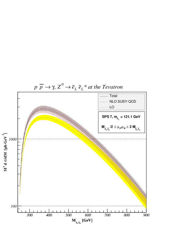
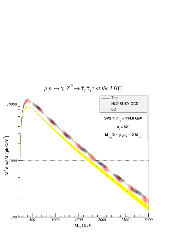
Figure 4.9: Invariant-mass distribution $M^{3}\,{\rm d}\sigma/{\rm d}M$ of $\tilde{e}_{L}$ pairs at the Tevatron (top) and $\tilde{\tau}_{1}$ pairs at the LHC (bottom) for the benchmark point SPS 7. We show the total NLL+NLO matched and the fixed-order NLO SUSY-QCD and LO QCD results, including the respective scale uncertainties as horizontally hatched, vertically hatched and shaded bands.

We take current masses and widths of the electroweak gauge bosons, electroweak mixing angle, electromagnetic fine structure constant and CKM matrix elements, as in Sec. 2.3.3 [149], and the physical masses of the SUSY particles and the mixing angles are obtained with the computer program SuSpect [202]. We choose one mSUGRA point, SPS 1a, and one GMSB point, SPS 7, with their associated model lines, as benchmarks for our numerical study [45]. SPS 1a is a typical mSUGRA point with an intermediate value of $\tan\beta=10$ and $\mu>0$, and the model line attached to it is specified by $m_{0}=-A_{0}=0.4\leavevmode\nobreak\ m_{1/2}$. For $m_{1/2}=250$ GeV, this SUSY-breaking scenario leads to light sleptons $\tilde{\tau}_{1}$, $\tilde{e}_{1}$, $\tilde{\tau}_{2}$, $\tilde{e}_{2}$, $\tilde{\nu}_{\tau}$ and $\tilde{\nu}_{e}$ with masses of 136.2, 146.4, 216.3, 212.3, 196.1 and 197.1 GeV and to heavy squarks with masses around 500-600 GeV. However, even if the top-squark mass eigenstate $\tilde{t}_{1}$ is slightly lighter, it does nonetheless not contribute to the virtual squark loops due to the negligible top-quark density in the proton (we consider flavour-conserving SUSY-loops in Fig. 4.8). SPS 7 is a GMSB scenario with a $\tilde{\tau}_{1}$ as the next-to-lightest SUSY particle and an effective SUSY-breaking scale $\Lambda=40$ TeV, $N_{\rm mes}=3$ messenger fields of mass $M_{\rm mes}=80$ TeV, $\tan\beta=15$, and $\mu>0$, which leads again to light sleptons with masses of 114.8, 121.1, 263.9, 262.1, 249.5 and 249.9 GeV, respectively, and even heavier squarks with masses around 800-900 GeV. Its model line is defined by $M_{\rm mes}=2\,\Lambda$. The slepton masses and mixing angles are actually quite similar for the SPS 1a mSUGRA and SPS 7 GMSB points, so that the corresponding production cross sections will not differ significantly. Slepton detection will, however, be slightly different in both scenarios, as the sleptons decay to a relatively massive neutralino LSP at SPS 1a, but to a very light gravitino LSP at SPS 7. The lightest tau slepton thus decays into a tau lepton and missing transverse energy.

Our cross sections are calculated for the Tevatron $p\bar{p}$-collider, as well as for the LHC $pp$-collider. For the LO (NLO and NLL) predictions, we use the LO 2001 [212] (NLO 2004 [207]) MRST-sets of parton distribution functions. For the NLO and NLL predictions, $\alpha_{s}$ is evaluated with the corresponding value of $\Lambda_{\overline{\rm MS}}^{n_{f}=5}=255$ MeV at two-loop accuracy. We fix the unphysical scales $\mu_{F}$ and $\mu_{R}$ equal to the invariant-mass $M$ of the slepton (slepton-sneutrino) pair.

The invariant-mass distribution $M^{3}{\rm d}\sigma/{\rm d}M$ for first- (and equal-mass second-) generation sleptons at the Tevatron is shown in the top panel of Fig. 4.9, and the one for (slightly lighter) third-generation sleptons at the LHC in the bottom panel of the same figure. In both cases, we have chosen the SPS 7 GMSB benchmark point. The differential cross section ${\rm d}\sigma/{\rm d}M$ has been multiplied by a factor $M^{3}$ in order to remove the leading mass dependence of propagator and phase space factors. As is to be expected for $P$-wave production of scalar particles, the distributions rise above the threshold at $\sqrt{s}=2m_{\tilde{l}}$ with the third power of the slepton velocity $\beta$, see Eq. (4.29), and peak at about 100 GeV above threshold (at 370 GeV for $M^{3}{\rm d}\sigma/{\rm d}M$ and 310 GeV for ${\rm d}\sigma/{\rm d}M$ for the Tevatron; 410 GeV and 300 GeV for the LHC), before falling off steeply due to the $s$-channel propagator and the decreasing parton luminosity. Furthermore, it can also be seen that the QCD corrections do not alter the $P$-wave velocity dependence close to threshold. At the Tevatron, the total and NLO SUSY-QCD predictions exceed the maximal LO cross section by 36 and 31%, respectively, whereas at the LHC, the maximal cross section increases by 28 and 27%. Threshold resummation effects are thus clearly more important at the Tevatron, where the hadronic centre-of-mass energy is limited and the scaling variable $\tau=M^{2}/s_{h}$ is closer to one, and they increase with $M$ to the right of both plots.

The maximal theoretical error is estimated in Fig. 4.9 by an independent variation of the factorization and renormalization scales between $M/2$ and $2M$. It is indicated as a shaded, vertically, and horizontally hatched band for the LO, NLO SUSY-QCD, and the total prediction. At LO, the only dependence comes from the factorization scale. It increases with the momentum-fraction $x$ of the partons in the proton or anti-proton and is therefore already substantial for small $M$ at the Tevatron, but only for larger $M$ at the LHC. At NLO, this dependence is reduced due to the factorization of initial-state singularities, but a strong additional dependence is introduced by the renormalization scale in the coupling $\alpha_{s}(\mu_{R})$. After resummation, this dependence is reduced as well, so that the total scale uncertainty at the Tevatron diminishes from 20%–35% for NLO to only 16%–17% for the matched resummed result. The reduction is, of course, more important in the large-$M$ region. At the LHC, where $\alpha_{s}$ is evaluated at a larger renormalization scale and is thus less sensitive to it, the corresponding numbers are 18%–25% and 15%–17%.

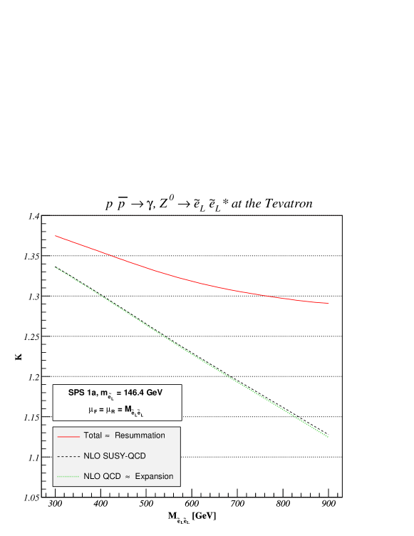
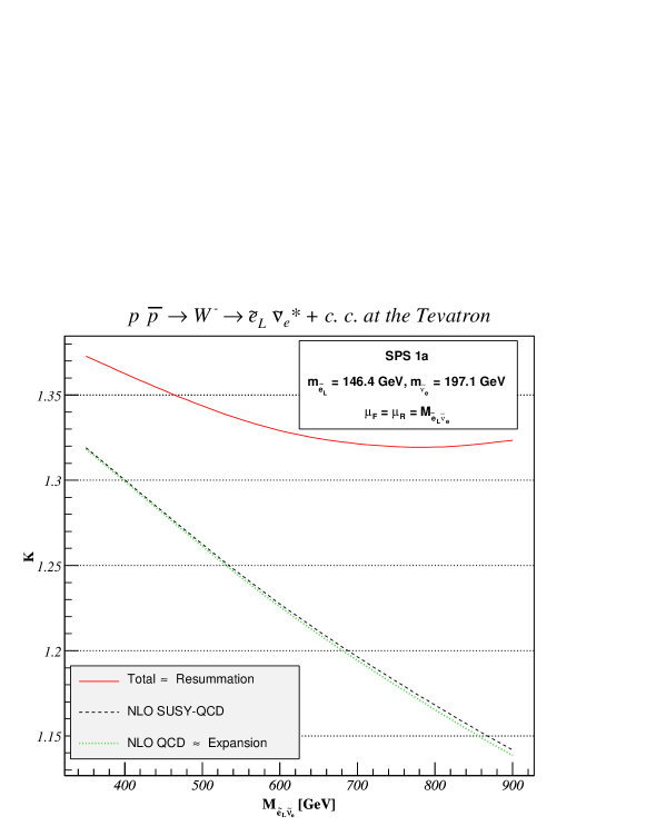
Figure 4.10: $K$-factors as defined in Eq. (4.71) for $\tilde{e}_{L}$ pair (top) and associated $\tilde{e}_{L}\tilde{\nu}_{e}^{\ast}$ production (bottom) at the Tevatron for the benchmark point SPS 1a. We show the total NLL+NLO matched result, which is almost identical to the purely resummed result at NLL, as well as the fixed-order NLO SUSY-QCD and QCD results. The latter practically coincides with the resummed result expanded up to NLO.

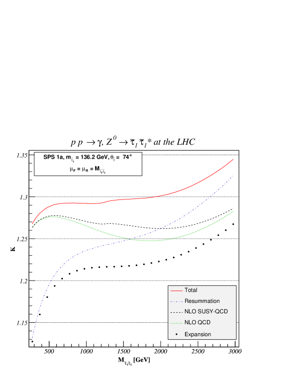
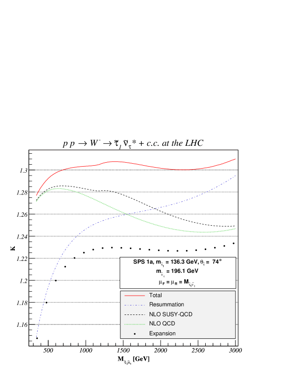
Figure 4.11: $K$-factors as defined in Eq. (4.71) for $\tilde{\tau}_{1}$ pair (top) and associated $\tilde{\tau}_{1}\tilde{\nu}_{\tau}^{\ast}$ production (bottom) at the LHC for the benchmark point SPS 1a. We show the total NLL+NLO matched result, the resummed result at NLL, the fixed-order NLO SUSY-QCD and QCD results, and the resummed result expanded up to NLO.

For the mSUGRA scenario SPS 1a, we show in Figs. 4.10 and 4.11 the cross section correction factors

$$K^{i}=\frac{{\rm d}\sigma^{i}/{\rm d}M}{{\rm d}\sigma^{\rm LO}/{\rm d}M},$$ (4.71)

where $i$ labels the corrections induced by NLO QCD (Eqs. (4.49) and (4.50)), additional NLO SUSY-QCD (Eqs. (4.62) and (4.63)), resummation (Eq. (4.64)), and the matched total contributions (Eq. (4.68)) as well as the fixed-order expansion (Eqs. (4.69) and (4.70)) of the resummation contribution as a function of the invariant-mass $M$. As one can see immediately, the mass-dependence of these corrections for charged-current associated production of sleptons and sneutrinos (lower parts of Figs. 4.10 and Fig. 4.11) does not differ substantially from the mass-dependence of the neutral-current production of slepton pairs (upper parts).

At the Tevatron (Fig. 4.10), where we are close to the threshold, resummation effects are already important at low $M$ (4%) and increase to sizeable 16% at large $M$. The NLO QCD result is thus dominated by large logarithms and coincides with the expanded result at the permille level. In addition, the relative importance of the (finite) SUSY-QCD contributions is reduced, and the total prediction coincides with the resummed prediction, since fixed-order and expanded contributions cancel each other in Eq. (4.68). We have also verified that exponentiating the finite ($N$-independent) terms collected in the coefficient function $C^{(1)}_{q\bar{q}^{(\prime)}}$, as proposed in [193] (see Eq. 4.67), leads only to a 0.6%–0.8% increase of the matched resummed result. The Tevatron being a $p\bar{p}$-collider, the total cross section is dominated by $q\bar{q}$-annihilation, and $qg$-scattering contributes at most 1% at small $M$ (or small $x$), where the gluon density is still appreciable. Integration over $M$ leads to total cross sections for the neutral (charged) current processes in Fig. 4.10 of 4.12 (3.92) fb in LO, 5.3 (4.96) fb in NLO (SUSY-)QCD, and 5.55 (5.28) fb for the matched resummed calculation. The corresponding (global) $K$-factors

$$K^{i}_{{\rm glob}} = \frac{\sigma^{i\leavevmode\nobreak\ \leavevmode\nobreak\ }}{\sigma^{\rm LO}}\leavevmode\nobreak\ =\leavevmode\nobreak\ \frac{\int{\rm d}M\,{\rm d}\sigma^{i\leavevmode\nobreak\ \leavevmode\nobreak\ }/{\rm d}M}{\int{\rm d}M\,{\rm d}\sigma^{\rm LO}/{\rm d}M}$$ (4.72)

are then 1.29 (1.27) at fixed-order and 1.35 (1.35) with resummation.

At the LHC, sleptons can be produced with relatively small invariant-mass $M$ compared to the total available centre-of-mass energy, so that $z=\tau/(x_{a}x_{b})=M^{2}/s\ll 1$ and the resummation of ($1-z$)-logarithms is less important. This is particularly true for the production of the light mass-eigenstates of mixing third-generation sleptons, as shown in Fig. 4.11. In the low-$M$ (left) parts of these plots, the total result is less than 0.5% larger than the NLO (SUSY-)QCD result. Only at large $M$ the logarithms become important and lead to a 7% increase of the $K$-factor with resummation over the fixed-order result. In this region, the resummed result approaches the total prediction, since the NLO QCD calculation is dominated by large logarithms and approaches the expanded resummed result. However, we are still far from the hadronic threshold region, and a consistent matching of both resummed and fixed-order contributions is needed. At low $M$, where finite terms dominate, the resummed contribution is close to its fixed-order expansion and disappears with $M$. In the intermediate-$M$ region, one can observe the effect of SUSY-QCD contributions, in particular the one coming from the $\tilde{q}\tilde{q}\tilde{g}$-vertex correction (lower left diagram in Fig. 4.8). As $M\geq 2m_{\tilde{q}}$, one crosses the threshold for squark pair production and observes a resonance in Fig. 4.11. As for the Tevatron, exponentiating the finite ($N$-independent) terms collected in the coefficient function $C^{(1)}_{q\bar{q}^{(\prime)}}$ leads only to a 1% increase of the matched resummed result. The LHC being a high-energy $pp$-collider, it has a significant gluon-luminosity, in particular at small $M$ (or $x$), and indeed the $qg$-subprocess changes (lowers) the total cross section by 7% at small $M$ and 3% at large $M$. After integration over $M$, we obtain total cross sections of 27 (9.59) fb in LO, 34.3 (12.3) fb in NLO SUSY-QCD, and 34.6 (12.5) fb for the resummed-improved result, corresponding to global $K$-factors of 1.28 for fixed-order and 1.29 for the matched resummed cross section for both processes. Resummation of large logarithms is thus not as important as for the Tevatron at the benchmark point SPS 1a.

4.4 Total cross section at NLO

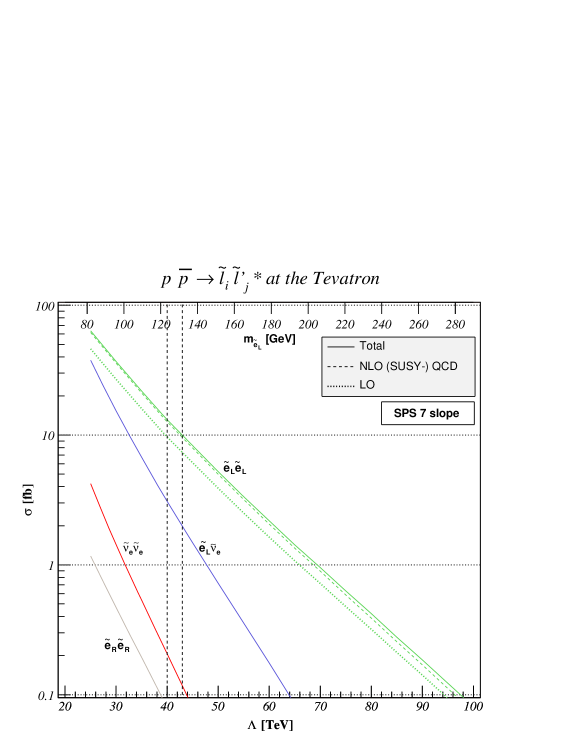
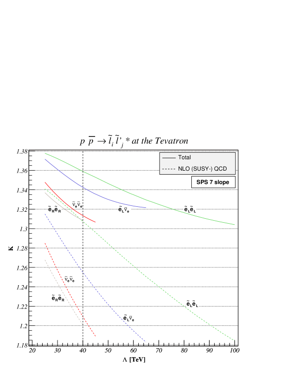
Figure 4.12: Total cross sections (top) and $K$-factors as defined in Eq. (4.72) (bottom) for first- (and second-) generation slepton pair and slepton-sneutrino associated production at the Tevatron along the model line attached to the SPS 7 benchmark point (vertical dashed line). We show the total NLL+NLO matched and the fixed-order NLO (SUSY-)QCD and LO QCD results.

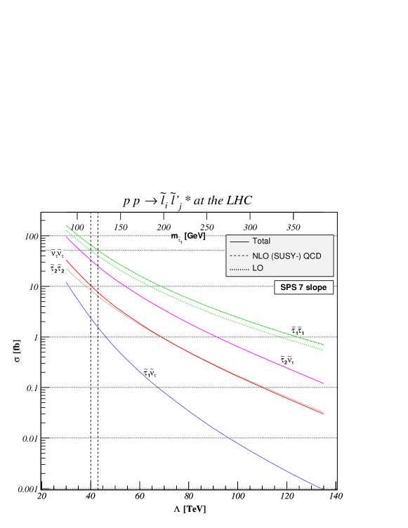
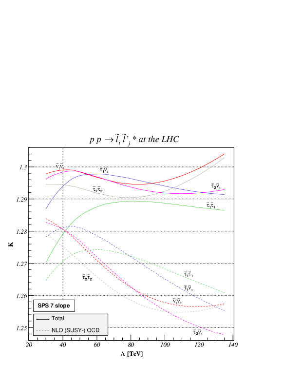
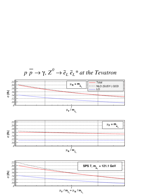
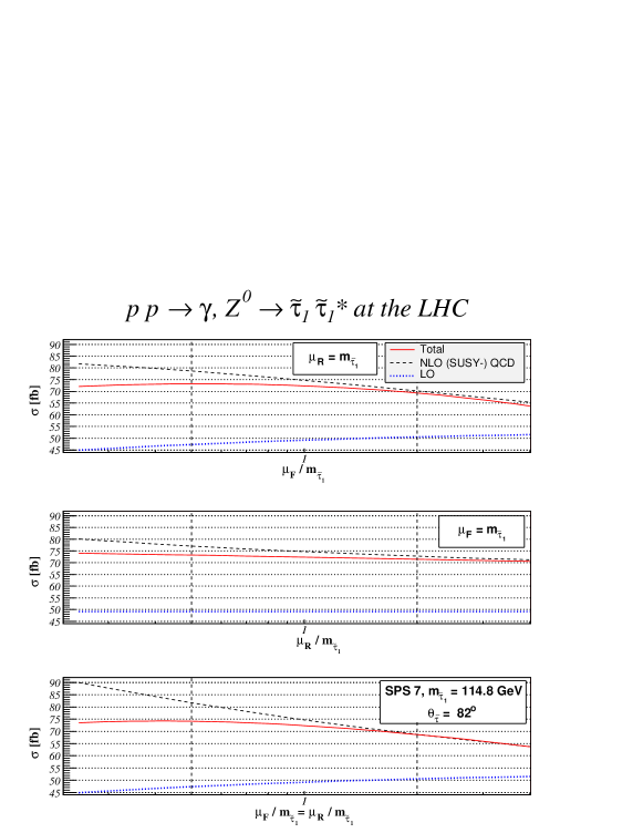
Figure 4.13: Total cross sections (top) and $K$-factors as defined in Eq. (4.72) (bottom) for third-generation slepton pair and slepton-sneutrino associated production at the LHC along the model line attached to the SPS 7 benchmark point (vertical dashed line). We show the total NLL+NLO matched and the fixed-order NLO (SUSY-)QCD and LO QCD results.

Figure 4.14: Dependence of the total cross section for first- (and second-) generation slepton pairs at the Tevatron on the factorization scale (top), renormalization scale (middle), and both scales (bottom) for the SPS 7 benchmark point.

Figure 4.15: Dependence of the total cross section for third-generation slepton pairs at the LHC on the factorization scale (top), renormalization scale (middle), and both scales (bottom) for the SPS 7 benchmark point.

In this section, we study the dependence of total, i.e. invariant-mass integrated, slepton pair and slepton-sneutrino cross sections on three different scales: first the dependence on the effective SUSY-breaking scale $\Lambda$ as defined in the GMSB model line SPS 7, and then the dependence on the renormalization and factorization scales $\mu_{R,F}$ at the point SPS 7. The benchmark point at $\Lambda=40$ TeV will be indicated in the figures where $\Lambda$ varies as a vertical dashed line, and we show in addition to the scale $\Lambda$ the mass scale of the produced charged slepton, ranging from 80 (87.5) to 280 (385) GeV for $\tilde{e}_{L}$ ($\tilde{\tau}_{1}$).

In Fig. 4.12, total cross sections (top) and $K$-factors (bottom) are shown at the Tevatron, which is expected to produce a total integrated luminosity of 4–8 fb^-1. Even for $\tilde{e}_{L}$ pair production the mass-range is limited to masses below 280 GeV, where the cross section reaches 0.1 fb and at most one event would be produced. NLO and resummation corrections are clearly important, as they increase the LO prediction by 18 to 28% (lower part of Fig. 4.12). At the SPS 7 benchmark point, the corrections would thus induce a shift in the selectron mass as deduced from a total cross section measurement by about 8 GeV (cf. the two dashed lines in the upper part of Fig. 4.12). By comparing the NLO and total predictions, one observes an increased importance of threshold resummation for heavier sleptons, as expected.

We show in Fig. 4.13 the total cross sections in the restricted range $\Lambda\leq 135$ TeV. The NLO and resummed corrections are again large (25–30%), but the resummation corrections only become appreciable for large SUSY-breaking scales (or slepton masses). The largest cross section is obtained for pair production of the light stau mass eigenstate, even though it has a large right-handed component. Conversely, the heavier stau mass eigenstate has a large left-handed component, so that its cross section is less suppressed. At the SPS 7 benchmark point, the corrections would again induce a shift in the slepton mass as deduced from a total cross section measurement by about 8 GeV, as can be seen for $\tilde{\tau}_{1}$ on the upper part of Fig. 4.13, cf. the two dashed lines.

Finally, we consider the theoretical uncertainty of invariant-mass integrated total cross sections at the Tevatron (Fig. 4.15) and the LHC (Fig. 4.15) as induced by variations of the factorization scale (top), renormalization scale (middle), or both (bottom). The $\mu_{R}$-dependence (middle), which is absent in LO, is first introduced in NLO, but then tamed by the resummation procedure. On the other hand, the logarithmic $\mu_{F}$-dependence (top), already present through the PDFs at LO, is overcompensated (reduced) at NLO for the LHC (Tevatron) and then (further) stabilized by resummation. This works considerably better at the LHC, where at least one quark PDF is sea-like and the PDFs are evaluated at lower $x$, than at the Tevatron, where both PDFs can be valence-like and are evaluated at relatively large $x$. In total, the theoretical uncertainty at the Tevatron (LHC), defined by the ratio of the cross section difference at $\mu_{F}=\mu_{R}=m_{\tilde{l}}/2$ and $\mu_{F}=\mu_{R}=2\,m_{\tilde{l}}$ over their sum, increases from 20 (7) % in LO to 29 (17) % in NLO, but is then reduced again to 23 (8) % for the resummed-improved prediction.

4.5 Jointly resummed results

We present here a joint treatment of the recoil corrections at small $q_{T}$ and the threshold-enhanced contributions near partonic threshold, allowing a complete understanding of the soft-gluon effects in differential distributions for slepton pair production at hadron colliders [80]. We use the joint formalism described in Sec. 3.4 and compare it to the $q_{T}$- and threshold resummation formalisms of Secs. 3.2.4 and 3.3.2. The fixed-order perturbative and the $q_{T}$- and threshold-resummed results for the transverse-momentum and invariant-mass distributions are those presented in the previous subsections, while the jointly-resummed matched cross section (see Eq. (3.119)) is

$$\frac{{\rm d}^{2}\sigma}{{\rm d}M^{2}\,{\rm d}q_{T}^{2}}(\tau) = \frac{{\rm d}^{2}\sigma^{({\rm F.O.})}}{{\rm d}M^{2}\,{\rm d}q_{T}^{2}}(\tau;\alpha_{s})+\frac{1}{2\,\pi\,i}\oint_{C_{N}}\frac{{\rm d}N}{2\pi i}\,\tau^{-N}\int\frac{b{\rm d}b}{2}J_{0}(q_{T}\,b)$$ (4.73)

$$\times\left[\frac{{\rm d}^{2}\sigma^{{\rm(res)}}}{{\rm d}M^{2}\,{\rm d}q_{T}^{2}}(N,b;\alpha_{s})-\frac{{\rm d}^{2}\sigma^{{\rm(exp)}}}{{\rm d}M^{2}\,{\rm d}q_{T}^{2}}(N,b;\alpha_{s})\right].\leavevmode\nobreak\$$

The resummed contribution is given by Eq. (3.108)

$$\frac{{\rm d}\sigma^{({\rm res})}}{{\rm d}M^{2}\,{\rm d}q^{2}_{T}} = \sum_{a,b}f_{a/h_{a}}(N+1,\mu_{F})\,f_{b/h_{b}}(N+1,\mu_{F})\,$$ (4.74)

$$\times \!\sum_{c}\!\mathcal{H}_{ab\to c\bar{c}}\Big{(}N;\alpha_{s}(\mu_{R}),\frac{M}{\mu_{R}},\frac{M}{\mu_{F}}\Big{)}\exp\Big{\{}\mathcal{G}_{c}(\ln\chi;\alpha_{s}(\mu_{R}),\frac{M}{\mu_{R}})\Big{\}},\leavevmode\nobreak\ \leavevmode\nobreak\ \leavevmode\nobreak\ \leavevmode\nobreak\ \leavevmode\nobreak\$$

while the expansion of the resummed component is (see Eq. (3.121))

$$\frac{{\rm d}\sigma^{({\rm exp})}}{{\rm d}M^{2}\,{\rm d}q^{2}_{T}} = \sum_{a,b}f_{a/h_{a}}(N+1,\mu_{F})\,f_{b/h_{b}}(N+1,\mu_{F})\,$$ (4.75)

$$\times \sum_{c}\sigma_{c{\bar{c}}}^{(0)}(M)\Bigg{\{}\delta_{ca}\delta_{{\bar{c}}b}+\sum_{n=1}^{\infty}\left(\frac{\alpha_{s}(\mu_{R})}{\pi}\right)^{n}$$

$$\times \Bigg{[}{\tilde{\Sigma}}_{ab\to c{\bar{c}}}^{(n)}\left(N,\ln\chi;\frac{M}{\mu_{R}},\frac{M}{\mu_{F}}\right)\!+\!\mathcal{H}_{ab\to c\bar{c}}^{(n)}\Big{(}N;\frac{M}{\mu_{R}},\frac{M}{\mu_{F}}\Big{)}\Bigg{]}\Bigg{\}}.\leavevmode\nobreak\$$

The $\mathcal{O}(\alpha_{s})$ coefficients of the perturbative functions $\mathcal{H}$, $\mathcal{G}$ and ${\tilde{\Sigma}}$, can be found in Sec. 3.4. We remind the reader only of the definition of the argument in the logarithm (see Eq. (3.99)),

$$\chi(\bar{N},\bar{b})=\bar{b}+\frac{\bar{N}}{1+\eta\,\bar{b}/\bar{N}}.\leavevmode\nobreak\$$ (4.76)

For the masses and widths of the electroweak gauge bosons, the electroweak mixing angle and the electromagnetic fine structure constant, we use the same values as in the previous section, i.e. those given by the latest version of the PDG review [149]. We focus our study on the production of a right-handed selectron pair at the LHC,

$$\begin{array}[]{c}q\bar{q}\to\gamma,Z^{0}\to\tilde{e}_{R}\,\tilde{e}^{\ast}_{R}.\end{array}$$ (4.78)

We use the MRST (2004) NLO set of parton distribution functions [207], $\alpha_{s}$ is evaluated at two-loop accuracy, and we allow $\mu_{F}$ and $\mu_{R}$ to vary between $M/2$ and $2M$ to estimate the perturbative uncertainty. We choose the mSUGRA benchmark point BFHK B (see Tab. 2.3) which gives, after the renormalization group evolution of the SUSY-breaking parameters performed by the SPheno computer program [156], a light ${\tilde{e}}_{R}$ of mass $m_{{\tilde{e}}_{R}}=186$ GeV and rather heavy squarks with masses around 800-850 GeV, except for top-squark mass eigenstate $\tilde{t}_{1}$ which is slightly lighter, but which nevertheless does not contribute to the virtual squark loops due to the negligible top-quark density in the proton.

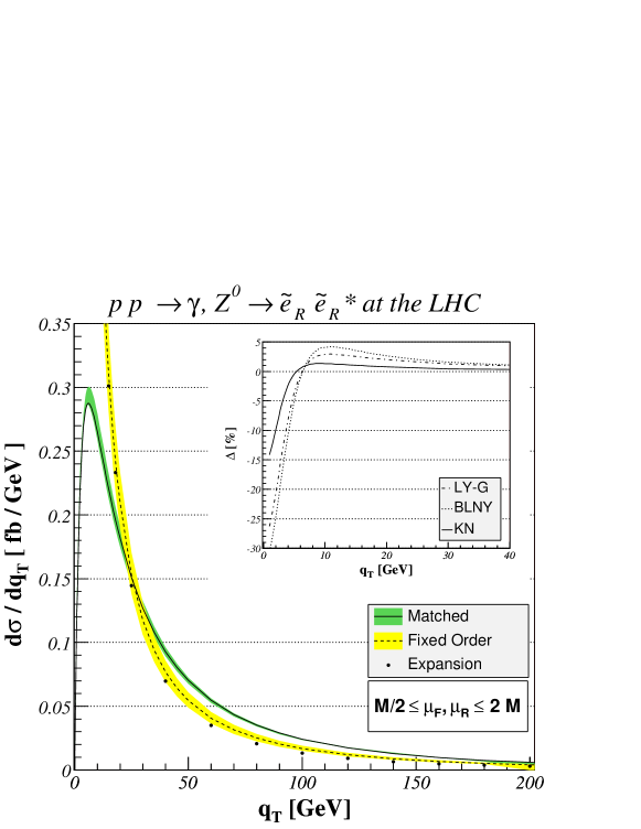
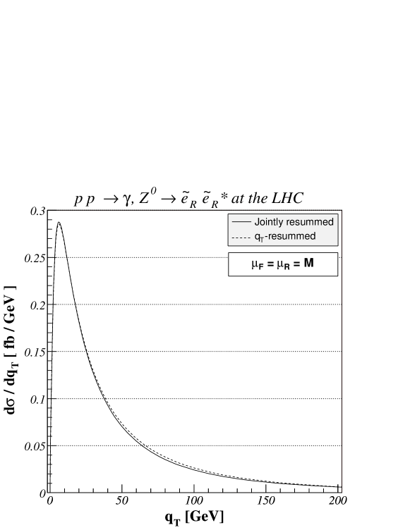
Figure 4.16: Transverse-momentum distribution for the process $pp\to\tilde{e}_{R}\,\tilde{e}_{R}^{\ast}$ at the LHC. NLL+LO matched result, LO result, asymptotic expansion of the resummation formula and $\Delta$-parameter are shown.

Figure 4.17: Transverse-momentum distribution for selectron pair production at the LHC ion the framework of joint and $q_{T}$ resummation.

In Fig. 4.17, we integrate the previous equations with respect to $M^{2}$, taking as lower limit the energy threshold for $\tilde{e}_{R}\tilde{e}_{R}^{\ast}$ production and as upper limit the hadronic energy, $\sqrt{s}_{h}$ = 14 TeV. We plot the LO result (dashed line) and the total NLL+LO matched result (solid line) with their uncertainty band relative to scale variation (yellow band for the LO result and green band for the NLL+LO result). The effect of resummation is clearly visible at small and intermediate values of $q_{T}$, the resummation-improved result reaching a value that is even 40% higher than the pure fixed-order result at $q_{T}=80$ GeV .

The asymptotic expansion of the resummation formula at LO (dotted line) is in good agreement with LO at small values of $q_{T}$, from which we can conclude that the cross section is clearly dominated by the logarithms that we are resumming in this kinematical region. In the intermediate-$q_{T}$ region, we can see that the expansion is slightly smaller than the fixed-order calculation. Since this effect was not present in $q_{T}$-resummation (see Fig. 4.5 in Sec. 4.2.2), we deduce that it is purely related to the threshold-enhanced contributions important in the large-$M$ region. It is also presented in Fig. 4.17, where we directly compare jointly- and $q_{T}$-matched results, the main difference between the two approaches relying indeed in this intermediate-$q_{T}$ region where the jointly-resummed cross section is 5%-10% lower than the $q_{T}$-resummed one for 50 GeV $<q_{T}<$ 100 GeV.

In Fig. 4.17, we estimate the scale dependence by an independent variation of the factorization and renormalization scales between $M/2$ and $2M$, and is clearly improved using resummation rather than pure fixed-order calculations. In the small and intermediate $q_{T}$-region the effect of scale variation is 10% for the LO result, while it is always less than 5% for the NLL+LO curve.

We also study the dependence of the total NLL+LO matched result on non-perturbative effects. We show the quantity $\Delta$ defined in Eq. (4.43),

$$\Delta=\frac{d\sigma^{\rm(res.+NP)}(\mu_{R}=\mu_{F}=M)-d\sigma^{(\rm res.)}(\mu_{R}=\mu_{F}=M)}{d\sigma^{(\rm res.)}(\mu_{R}=\mu_{F}=M)},$$ (4.79)

as a function of the transverse momentum of the slepton pair. The parameter $\Delta$ gives thus an estimate of the contributions from the different NP parameterizations (LY-G, BLNY, KN) that we included in the resummed formula, which can be found in Eqs. (3.32), (3.33) and (3.34). They are under good control, since they are always less than 5% for $q_{T}>$ 5 GeV and thus considerably smaller than the resummation effects.

The invariant-mass distribution $M^{3}{\rm d}\sigma/{\rm d}M$ for $\tilde{e}_{R}$-pair production at the LHC is obtained by integrating the equations given above with respect to the transverse-momentum $q_{T}$, and is shown in Fig. 4.19. As in the previous section, the differential cross section ${\rm d}\sigma/{\rm d}M$ has been multiplied by a factor $M^{3}$ in order to remove the leading mass dependence of propagator and phase space factors. We can again see the $P$-wave behaviour relative to the production of scalar particles, since the invariant-mass distribution rises above the threshold at $\sqrt{s}=2m_{\tilde{e}_{R}}$ with the third power of the slepton velocity and peaks at about 200 GeV above threshold (both for $M^{3}{\rm d}\sigma/{\rm d}M$ and the not shown ${\rm d}\sigma/{\rm d}M$ differential distribution), before falling off steeply due to the $s$-channel propagator and the decreasing parton luminosity. Let us note that we use the MRST LO 2001 [212] set of parton distribution functions for the LO predictions.

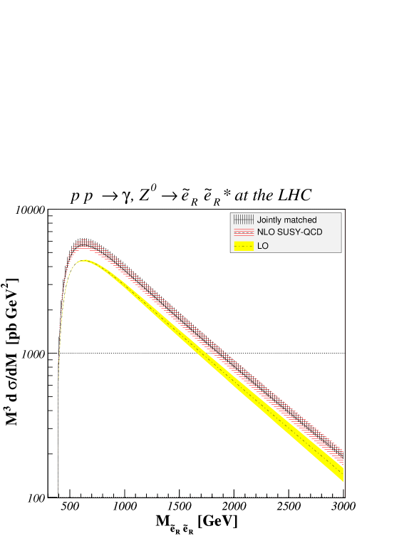
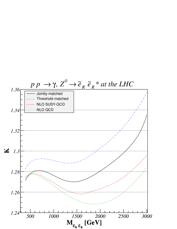
Figure 4.18: Invariant-mass distribution $M^{3}\,{\rm d}\sigma/{\rm d}M$ of $\tilde{e}_{R}$ pairs at the LHC. We show the total NLL+NLO matched and the fixed-order NLO SUSY-QCD and LO QCD results, including the respective scale uncertainties as vertically hatched, horizontally hatched and shaded bands.

Figure 4.19: $K$-factors as defined in Eq. (4.80) for $\tilde{e}_{R}$ pair production at the LHC. We show the total NLL+NLO jointly- and threshold-matched result, as well as the fixed-order NLO SUSY-QCD and QCD results.

In the large-$M$ region, the resummed cross section is 30% higher than the leading-order cross section, but this represents only a 3% increase with respect to the NLO SUSY-QCD result. In the small-$M$ region, much further then from the hadronic threshold, resummation effects are rather limited, inducing a modification of the NLO results smaller than 1%.

The shaded, horizontally and vertically shaded bands in Fig. 4.19 represent the theoretical uncertainties for the LO, NLO SUSY-QCD, and the jointly-matched predictions. At LO, the dependence coming only from the factorization scale increases with the momentum-fraction $x$ of the partons in the proton (i.e. with $M$), being thus larger in the right part of the figure, but this dependence is largely reduced at NLO due to the factorization of initial-state singularities in the PDFs. However, we add the dependence due to the renormalization scale in the coupling $\alpha_{s}(\mu_{R})$, leading to a total variation of about 7%-11%. After resummation, the total scale uncertainty is finally reduced to only 7%-8% for the matched result, the reduction being of course more important in the large-$M$ region, where the resummation effects are more important.

In Fig. 4.19, we show the cross section correction factors

$$K^{i}=\frac{{\rm d}\sigma^{i}/{\rm d}M}{{\rm d}\sigma^{\rm LO}/{\rm d}M}$$ (4.80)

as a function of the invariant-mass $M$. $i$ labels the corrections induced by NLO QCD, NLO SUSY-QCD, joint- and threshold-resummation, these two last calculations being matched with the NLO SUSY-QCD result.

At small invariant mass $M$, the resummation is less important, since we are quite far from the hadronic threshold, as shown in the left part of the plot. At larger $M$, the logarithms become important and lead to a larger increase of the resummed $K$-factors over the fixed-order one. We also show the difference between threshold and joint resummations, which is only about one or two percents. It is due to the choice of the Sudakov form factor $\mathcal{G}$ and of the $\mathcal{H}$-function, which reproduces correctly transverse-momentum resummation in the limit of $b\to\infty$, $N$ being fixed, but which presents some differences with the pure threshold limit $b\to 0$ and $N\to\infty$, as it was the case for joint resummation for Higgs and electroweak boson production [77, 78]. However, this effect is under good control, since it is much smaller than the theoretical scale uncertainty of about 7%.

  

Chapter 5 Squark and gaugino production and decays at hadron colliders

In many models, the non-coloured charginos and neutralinos belong to the class of the lightest supersymmetric particles, their low masses counterbalancing the small weak cross sections for direct production. Theoretically, full NLO SUSY-QCD calculations have been performed [40], while experimentally, their subsequent decay to gold-plated trilepton signatures [213, 214] have been exploited in several CDF and D0 analyses at the Tevatron [215, 216, 217, 218, 219] and will be investigated at the LHC [220, 221]. Due to their strong coupling, squarks should be abundantly produced at hadron colliders, and hadroproduction cross sections and decay has therefore been studied in detail at NLO SUSY-QCD [34]. The production of top [35] and bottom [95] squarks with large helicity mixing has received particular attention, and both QCD one-loop and electroweak tree-level contributions have been calculated for non-diagonal, diagonal and mixed top and bottom squark pair production [96]. Very recently, flavour violation has been considered in the context of collider searches [97]. Concerning the associated production of squarks and gauginos, NLO SUSY-QCD cross sections in cMFV SUSY have been calculated some times ago [37] and generalized to NMFV scenarios [97].

In the following, we use for the sake of simplicity the generic notation

$$\left\{\mathcal{C}^{1}_{abc},\mathcal{C}^{2}_{abc}\right\}=\left\{L_{abc},R_{abc}\right\}$$ (5.1)

for the couplings defined in Sec. 2.4, while the propagators appearing as mass-subtracted Mandelstam variables read

$$\begin{array}[]{l c l c l c l c}s_{w}&=&s-m_{W}^{2}&,\nobreak\leavevmode&s_{z}&=&s-m_{Z}^{2}&,\\ t_{\tilde{\chi}^{0}_{k}}&=&t-m_{\tilde{\chi}^{0}_{k}}^{2}&,\nobreak\leavevmode&u_{\tilde{\chi}^{0}_{k}}&=&u-m_{\tilde{\chi}^{0}_{k}}^{2}&,\\ t_{\tilde{\chi}_{j}}&=&t-m_{\tilde{\chi}^{\pm}_{j}}^{2}&,\nobreak\leavevmode&u_{\tilde{\chi}_{j}}&=&u-m_{\tilde{\chi}^{\pm}_{j}}^{2}&,\\ t_{\tilde{g}}&=&t-m^{2}_{\tilde{g}}&,\nobreak\leavevmode&u_{\tilde{g}}&=&u-m^{2}_{\tilde{g}}&,\\ t_{\tilde{q}_{i}}&=&t-m_{\tilde{q}_{i}}^{2}&,\nobreak\leavevmode&u_{\tilde{q}_{i}}&=&u-m_{\tilde{q}_{i}}^{2}&.\end{array}$$ (5.7)

5.1 NMFV squark-antisquark pair hadroproduction

5.1.1 Analytical results

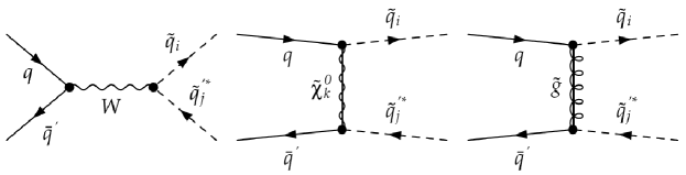
Figure 5.1: Tree-level Feynman diagrams for the production of charged squark-antisquark pairs in quark-antiquark collisions.

In NMFV SUSY, the production of charged squark-antisquark pairs

$$q(h_{a},p_{a})\,\bar{q}^{\prime}(h_{b},p_{b})\to\tilde{u}_{i}(p_{1})\,\tilde{d}^{\ast}_{j}(p_{2}),$$ (5.8)

where $i,j=1,...,6$ label up- and down-type squark mass eigenstates, $h_{a,b}$ helicities, and $p_{a,b,1,2}$ four-momenta, proceeds from an equally charged quark-antiquark initial state through the tree-level Feynman diagrams shown in Fig. 5.1. The corresponding cross section can be written in a compact way as [97]

$$\frac{{\rm d}\hat{\sigma}^{q\bar{q}^{\prime}}_{h_{a},h_{b}}}{dt} = (1-h_{a})(1+h_{b})\Bigg{[}\frac{\mathcal{W}}{s_{w}^{2}}+\bigg{(}\sum_{k,l=1,...,4}\frac{\mathcal{N}^{kl}_{11}}{t_{\tilde{\chi}^{0}_{k}}\,t_{\tilde{\chi}^{0}_{l}}}\bigg{)}+\frac{\mathcal{G}_{11}}{t_{\tilde{g}}^{2}}+\bigg{(}\sum_{k=1,...,4}\frac{\mathcal{[NW]}^{k}}{t_{\tilde{\chi}^{0}_{k}}\,s_{w}}\bigg{)}$$ (5.9)

$$+ \frac{\mathcal{[GW]}}{t_{\tilde{g}}\,s_{w}}\Bigg{]}+(1-h_{a})(1-h_{b})\Bigg{[}\bigg{(}\sum_{k,l=1,...,4}\frac{\mathcal{N}^{kl}_{12}}{t_{\tilde{\chi}^{0}_{k}}\,t_{\tilde{\chi}^{0}_{l}}}\bigg{)}+\frac{\mathcal{G}_{12}}{t_{\tilde{g}}^{2}}\Bigg{]}$$

$$+ (1+h_{a})(1+h_{b})\Bigg{[}\bigg{(}\sum_{k,l=1,...,4}\frac{\mathcal{N}^{kl}_{21}}{t_{\tilde{\chi}^{0}_{k}}\,t_{\tilde{\chi}^{0}_{l}}}\bigg{)}+\frac{\mathcal{G}_{21}}{t_{\tilde{g}}^{2}}\Bigg{]}$$

$$+ (1+h_{a})(1-h_{b})\Bigg{[}\bigg{(}\sum_{k,l=1,...,4}\frac{\mathcal{N}^{kl}_{22}}{t_{\tilde{\chi}^{0}_{k}}\,t_{\tilde{\chi}^{0}_{l}}}\bigg{)}+\frac{\mathcal{G}_{22}}{t_{\tilde{g}}^{2}}\Bigg{]}$$

thanks to the form factors

$$\mathcal{W} = \frac{\pi\,\alpha^{2}}{16\,x_{W}^{2}\,(1-x_{W})^{2}\,s^{2}}\left|L^{\ast}_{qq^{\prime}W}\,L_{\tilde{u}_{i}\tilde{d}_{j}W}\right|^{2}\left(u\,t-m^{2}_{\tilde{u}_{i}}\,m^{2}_{\tilde{d}_{j}}\right),\leavevmode\nobreak\$$

$$\mathcal{N}_{mn}^{kl} = \frac{\pi\,\alpha^{2}}{x_{W}^{2}\,(1-x_{W})^{2}\,s^{2}}\mathcal{C}^{n}_{\tilde{d}_{j}q^{\prime}\tilde{\chi}_{k}^{0}}\,\mathcal{C}^{m\ast}_{\tilde{u}_{i}q\tilde{\chi}_{k}^{0}}\,\mathcal{C}^{n\ast}_{\tilde{d}_{j}\tilde{\chi}_{l}^{0}}\,\mathcal{C}^{m}_{\tilde{u}_{i}q\tilde{\chi}_{l}^{0}}\,$$

$$\times \Bigg{[}\left(u\,t-m^{2}_{\tilde{u}_{i}}\,m^{2}_{\tilde{d}_{j}}\right)\delta_{mn}+\left(m_{\tilde{\chi}^{0}_{k}}\,m_{\tilde{\chi}^{0}_{l}}\,s\right)\left(1-\delta_{mn}\right)\Bigg{]},\leavevmode\nobreak\$$

$$\mathcal{G}_{mn} = \frac{2\,\pi\,\alpha_{s}^{2}}{9\,s^{2}}\left|\mathcal{C}^{n\ast}_{\tilde{d}_{j}q^{\prime}\tilde{g}}\,\mathcal{C}^{m}_{\tilde{u}_{i}q\tilde{g}}\right|^{2}\Bigg{[}\left(u\,t-m^{2}_{\tilde{u}_{i}}\,m^{2}_{\tilde{d}_{j}}\right)\delta_{mn}+\left(m_{\tilde{g}}^{2}\,s\right)\left(1-\delta_{mn}\right)\Bigg{]},\leavevmode\nobreak\$$

$$\mathcal{[NW]}^{k} = \frac{\pi\,\alpha^{2}}{6\,x_{W}^{2}\,(1\!-\!x_{W})^{2}\,s^{2}}\,{\rm Re}\!\left[\!L^{\ast}_{qq^{\prime}W}L_{\tilde{u}_{i}\tilde{d}_{j}W}L_{\tilde{u}_{i}q\tilde{\chi}_{k}^{0}}L^{\ast}_{\tilde{q}_{j}q^{\prime}\tilde{\chi}_{k}^{0}}\right]\!\left(\!u\,t\!-\!m^{2}_{\tilde{u}_{i}}\,m^{2}_{\tilde{d}_{j}}\!\right),\!$$

$$\mathcal{[GW]} = \frac{4\,\pi\,\alpha_{s}\,\alpha}{18\,x_{W}\,(1\!-\!x_{W})\,s^{2}}\,{\rm Re}\!\left[\!L^{\ast}_{\tilde{u}_{i}q\tilde{g}}L_{\tilde{d}_{j}q^{\prime}\tilde{g}}L^{\ast}_{qq^{\prime}W}L_{\tilde{u}_{i}\tilde{d}_{j}W}\right]\!\left(\!u\,t\!-\!m^{2}_{\tilde{u}_{i}}\,m^{2}_{\tilde{d}_{j}}\!\right),\!$$ (5.10)

which combine coupling constants and Dirac traces of the squared and interference diagrams. In cMFV SUSY, superpartners of heavy flavours can only be produced through the purely left-handed $s$-channel $W$-exchange, since the $t$-channel diagrams are suppressed by the small bottom and negligible top quark densities in the proton, and one recovers the result in Ref. [96]. In NMFV, $t$-channel exchanges can, however, contribute to heavy-flavour final state production from light-flavour initial states and even become dominant, due to the strong gluino coupling.

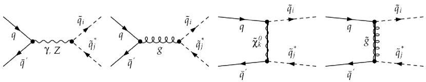
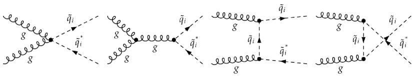
Figure 5.2: Tree-level Feynman diagrams for the production of neutral squark-antisquark pairs in quark-antiquark (top) and gluon-gluon collisions (bottom).

Neutral squark-antisquark pair production in NMFV proceeds either from equally neutral quark-antiquark initial states

$$q(h_{a},p_{a})\,\bar{q}^{\prime}(h_{b},p_{b})\to\tilde{q}_{i}(p_{1})\,\tilde{q}^{\ast}_{j}(p_{2})$$ (5.11)

through the five different gauge-boson/gaugino exchanges shown in Fig. 5.2 (top) or from gluon-gluon initial states

$$g(h_{a},p_{a})\,g(h_{b},p_{b})\to\tilde{q}_{i}(p_{1})\,\tilde{q}^{\ast}_{i}(p_{2})$$ (5.12)

through the purely strong couplings shown in Fig. 5.2 (bottom). The differential cross section for quark-antiquark scattering [97]

$$\frac{{\rm d}\hat{\sigma}^{q\bar{q}^{\prime}}_{h_{a},h_{b}}}{dt} = (1-h_{a})(1+h_{b})\Bigg{[}\frac{\mathcal{Y}}{s^{2}}+\frac{\mathcal{Z}_{1}}{s_{z}^{2}}+\frac{\mathcal{G}}{s^{2}}+\frac{\tilde{\mathcal{G}}_{11}}{t_{\tilde{g}}^{2}}+\frac{\mathcal{[YZ]}_{1}}{s\,s_{z}}+\frac{[\tilde{\mathcal{G}}\mathcal{Y}]_{1}}{t_{\tilde{g}}\,s}+\frac{[\tilde{\mathcal{G}}\mathcal{Z}]_{1}}{t_{\tilde{g}}\,s_{z}}$$

$$+ \frac{[\tilde{\mathcal{G}}\mathcal{G}]_{1}}{t_{\tilde{g}}\,s}+\sum_{k,l=1,...,4}\bigg{(}\frac{\mathcal{N}^{kl}_{11}}{t_{\tilde{\chi}^{0}_{k}}\,t_{\tilde{\chi}^{0}_{l}}}\bigg{)}+\sum_{k=1,...,4}\bigg{(}\frac{\mathcal{[NY]}^{k}_{1}}{t_{\tilde{\chi}^{0}_{k}}\,s}+\frac{\mathcal{[NZ]}^{k}_{1}}{t_{\tilde{\chi}^{0}_{k}}\,s_{z}}+\frac{\mathcal{[NG]}^{k}_{1}}{t_{\tilde{\chi}^{0}_{k}}\,s}\bigg{)}\Bigg{]}$$

$$+ (1+h_{a})(1-h_{b})\Bigg{[}\frac{\mathcal{Y}}{s^{2}}+\frac{\mathcal{Z}_{2}}{s_{z}^{2}}+\frac{\mathcal{G}}{s^{2}}+\frac{\tilde{\mathcal{G}}_{22}}{t_{\tilde{g}}^{2}}+\frac{\mathcal{[YZ]}_{2}}{s\,s_{z}}+\frac{[\tilde{\mathcal{G}}\mathcal{Y}]_{2}}{t_{\tilde{g}}\,s}+\frac{[\tilde{\mathcal{G}}\mathcal{Z}]_{2}}{t_{\tilde{g}}\,s_{z}}$$

$$+ \frac{[\tilde{\mathcal{G}}\mathcal{G}]_{2}}{t_{\tilde{g}}\,s}+\sum_{k,l=1,...,4}\bigg{(}\frac{\mathcal{N}^{kl}_{22}}{t_{\tilde{\chi}^{0}_{k}}\,t_{\tilde{\chi}^{0}_{l}}}\bigg{)}+\sum_{k=1,...,4}\bigg{(}\frac{\mathcal{[NY]}^{k}_{2}}{t_{\tilde{\chi}^{0}_{k}}\,s}+\frac{\mathcal{[NZ]}^{k}_{2}}{t_{\tilde{\chi}^{0}_{k}}\,s_{z}}+\frac{\mathcal{[NG]}^{k}_{2}}{t_{\tilde{\chi}^{0}_{k}}\,s}\bigg{)}\Bigg{]}$$

$$+ (1-h_{a})(1-h_{b})\Bigg{[}\frac{\tilde{\mathcal{G}}_{12}}{t_{\tilde{g}}^{2}}+\sum_{k,l=1,...,4}\bigg{(}\frac{\mathcal{N}^{kl}_{12}}{t_{\tilde{\chi}^{0}_{k}}\,t_{\tilde{\chi}^{0}_{l}}}\bigg{)}\Bigg{]}\hskip 71.13188pt$$ (5.13)

$$+ (1+h_{a})(1+h_{b})\Bigg{[}\frac{\tilde{\mathcal{G}}_{21}}{t_{\tilde{g}}^{2}}+\sum_{k,l=1,...,4}\bigg{(}\frac{\mathcal{N}^{kl}_{21}}{t_{\tilde{\chi}^{0}_{k}}\,t_{\tilde{\chi}^{0}_{l}}}\bigg{)}\Bigg{]}$$

involves many different form factors,

$$\mathcal{Y} = \frac{\pi\,\alpha^{2}\,e_{q}^{2}\,e_{\tilde{q}}^{2}\,\delta_{ij}\,\delta_{qq^{\prime}}}{s^{2}}\left(u\,t-m^{2}_{\tilde{q}_{i}}\,m^{2}_{\tilde{q}_{j}^{\prime}}\right),\leavevmode\nobreak\$$

$$\mathcal{Z}_{m} = \frac{\pi\,\alpha^{2}}{16\,s^{2}\,x_{W}^{2}(1-x_{W})^{2}}\left|L_{\tilde{q}_{i}\tilde{q}_{j}Z}+R_{\tilde{q}_{i}\tilde{q}_{j}Z}\right|^{2}\,\left(C^{m}_{qq^{\prime}Z}\right)^{2}\left(u\,t-m^{2}_{\tilde{q}_{i}}\,m^{2}_{\tilde{q}_{j}^{\prime}}\right),\leavevmode\nobreak\$$

$$\mathcal{G} = \frac{2\,\pi\,\alpha_{s}^{2}\,\delta_{ij}\,\delta_{qq^{\prime}}}{9\,s^{2}}\left(u\,t-m^{2}_{\tilde{q}_{i}}\,m^{2}_{\tilde{q}_{j}^{\prime}}\right),\leavevmode\nobreak\$$

$$\mathcal{N}_{mn}^{kl} = \frac{\pi\,\alpha^{2}}{x_{W}^{2}\,(1-x_{W})^{2}\,s^{2}}\,\mathcal{C}^{m\ast}_{\tilde{q}_{i}q\tilde{\chi}_{k}^{0}}\,\mathcal{C}^{m}_{\tilde{q}_{i}q\tilde{\chi}_{l}^{0}}\,\mathcal{C}^{n}_{\tilde{q}_{j}q^{\prime}\tilde{\chi}_{k}^{0}}\mathcal{C}^{n\ast}_{\tilde{q}_{j}q^{\prime}\tilde{\chi}_{l}^{0}}$$

$$\times \Bigg{[}\left(u\,t-m^{2}_{\tilde{q}_{i}}\,m^{2}_{\tilde{q}_{j}}\right)\,\delta_{mn}+\left(m_{\tilde{\chi}^{0}_{k}}\,m_{\tilde{\chi}^{0}_{l}}\,s\right)\,\left(1-\delta_{mn}\right)\Bigg{]},\leavevmode\nobreak\$$

$$\tilde{\mathcal{G}}_{mn} = \frac{2\,\pi\,\alpha_{s}^{2}}{9\,s^{2}}\,\left|\mathcal{C}^{m}_{\tilde{q}_{i}q\tilde{g}}\,\mathcal{C}^{n\ast}_{\tilde{q}_{j}q^{\prime}\tilde{g}}\right|^{2}\Bigg{[}\left(u\,t-m^{2}_{\tilde{q}_{i}}\,m^{2}_{\tilde{q}_{j}}\right)\,\delta_{mn}+\left(m_{\tilde{g}}^{2}\,s\right)\,\left(1-\delta_{mn}\right)\Bigg{]},\leavevmode\nobreak\$$

$$\mathcal{[YZ]}_{m} = \frac{\pi\,\alpha^{2}\,e_{q}\,e_{\tilde{q}}\,\delta_{ij}\,\delta_{qq^{\prime}}}{2\,s^{2}\,x_{W}(1-x_{W})}\,{\rm Re}\left[L_{\tilde{q}_{i}\tilde{q}_{j}Z}+R_{\tilde{q}_{i}\tilde{q}_{j}Z}\right]\,C^{m}_{qq^{\prime}Z}\left(u\,t-m^{2}_{\tilde{q}_{i}}\,m^{2}_{\tilde{q}_{j}^{\prime}}\right),\leavevmode\nobreak\$$

$$\mathcal{[NY]}_{m}^{k} = \frac{2\,\pi\,\alpha^{2}\,e_{q}\,e_{\tilde{q}}\,\delta_{ij}\,\delta_{qq^{\prime}}}{3\,x_{W}\,(1-x_{W})\,s^{2}}\,{\rm Re}\left[\mathcal{C}^{m}_{\tilde{q}_{i}q\tilde{\chi}_{k}^{0}}\,\mathcal{C}^{m\ast}_{\tilde{q}_{j}q^{\prime}\tilde{\chi}_{k}^{0}}\right]\left(u\,t-m^{2}_{\tilde{q}_{i}}\,m^{2}_{\tilde{q}_{j}}\right),\leavevmode\nobreak\$$

$$\mathcal{[NZ]}_{m}^{k} = \frac{\pi\,\alpha^{2}}{6\,x_{W}^{2}\,(1-x_{W})^{2}\,s^{2}}\,{\rm Re}\left[\mathcal{C}^{m}_{\tilde{q}_{i}q\tilde{\chi}_{k}^{0}}\,\mathcal{C}^{m\ast}_{\tilde{q}_{j}q^{\prime}\tilde{\chi}_{k}^{0}}\left(L_{\tilde{q}_{i}\tilde{q}_{j}Z}+R_{\tilde{q}_{i}\tilde{q}_{j}Z}\right)\right]\,\mathcal{C}^{m}_{qq^{\prime}Z}\,$$

$$\times \left(u\,t-m^{2}_{\tilde{q}_{i}}\,m^{2}_{\tilde{q}_{j}}\right),\leavevmode\nobreak\$$

$$\mathcal{[NG]}_{m}^{k} = \frac{8\,\pi\,\alpha\,\alpha_{s}\,\delta_{ij}\,\delta_{qq^{\prime}}}{9\,x_{W}\,(1-x_{W})\,s^{2}}\,{\rm Re}\left[\mathcal{C}^{m}_{\tilde{q}_{i}q\tilde{\chi}_{k}^{0}}\,\mathcal{C}^{m\ast}_{\tilde{q}_{j}q^{\prime}\tilde{\chi}_{k}^{0}}\right]\left(u\,t-m^{2}_{\tilde{q}_{i}}\,m^{2}_{\tilde{q}_{j}}\right),\leavevmode\nobreak\$$

$$\big{[}\tilde{\mathcal{G}}\mathcal{G}\big{]}_{m} = -\frac{4\,\pi\,\alpha_{s}^{2}\,\delta_{ij}\,\delta_{qq^{\prime}}}{27\,s^{2}}\,{\rm Re}\left[\mathcal{C}^{m\ast}_{\tilde{q}_{i}q\tilde{g}}\,\mathcal{C}^{m}_{\tilde{q}_{j}q^{\prime}\tilde{g}}\right]\left(u\,t-m^{2}_{\tilde{q}_{i}}\,m^{2}_{\tilde{q}_{j}}\right),\leavevmode\nobreak\$$

$$\mathcal{[\tilde{\mathcal{G}}Z]}_{m} = \frac{2\,\pi\,\alpha\,\alpha_{s}}{9\,x_{W}(1\!-\!x_{W})\,s^{2}}\,{\rm Re}\left[\mathcal{C}^{m\ast}_{\tilde{q}_{i}q\tilde{g}}\mathcal{C}^{m}_{\tilde{q}_{j}q^{\prime}\tilde{g}}\left(\!L_{\tilde{q}_{i}\tilde{q}_{j}Z}\!+\!R_{\tilde{q}_{i}\tilde{q}_{j}Z}\right)\!\right]\mathcal{C}^{m}_{qq^{\prime}Z}\,\left(\!u\,t\!-\!m^{2}_{\tilde{q}_{i}}\,m^{2}_{\tilde{q}_{j}}\!\right),$$

$$\mathcal{[\tilde{\mathcal{G}}Y]}_{m} = \frac{8\,\pi\,\alpha\,\alpha_{s}\,e_{q}\,e_{\tilde{q}}\,\delta_{ij}\,\delta_{qq^{\prime}}}{9\,s^{2}}\,{\rm Re}\left[\mathcal{C}^{m\ast}_{\tilde{q}_{i}q\tilde{g}}\,\mathcal{C}^{m}_{\tilde{q}_{j}q^{\prime}\tilde{g}}\right]\left(u\,t-m^{2}_{\tilde{q}_{i}}\,m^{2}_{\tilde{q}_{j}}\right),\leavevmode\nobreak\$$ (5.14)

since only very few interferences (those between strong and electroweak channels of the same propagator type) are eliminated due to colour conservation. On the other hand, the gluon-initiated cross section

$$\frac{{\rm d}\hat{\sigma}^{gg}_{h_{a},h_{b}}}{dt}\!=\!\frac{\pi\alpha_{s}^{2}}{128s^{2}}\!\left[\!24\left(\!1\!-\!2\frac{t_{\tilde{q}_{i}}u_{\tilde{q}_{i}}}{s^{2}}\!\right)\!-\!\frac{8}{3}\!\right]\!\!\left[\!(1\!-\!h_{a}h_{b})\!-\!2\frac{sm_{\tilde{q}_{i}}^{2}}{t_{\tilde{q}_{i}}u_{\tilde{q}_{i}}}\!\left(\!(1\!-\!h_{a}h_{b})\!-\!\frac{sm_{\tilde{q}_{i}}^{2}}{t_{\tilde{q}_{i}}u_{\tilde{q}_{i}}}\!\right)\!\right]\leavevmode\nobreak\$$ (5.15)

involves only the strong coupling constant and is thus quite compact. In the case of cMFV, our results agree with those in Ref. [96] for diagonal and non diagonal squark helicities in the final state. Diagonal production of identical squark-antisquark mass eigenstates is, of course, dominated by the strong quark-antiquark and gluon-gluon channels. Their relative importance depends on the partonic luminosity and thus on the type and energy of the hadron collider under consideration. Non-diagonal production of squarks of different helicity or flavour involves only electroweak and gluino-mediated quark-antiquark scattering, and the relative importance of these processes depends largely on the gluino mass.

5.1.2 Numerical results

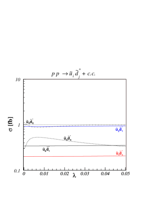
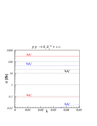
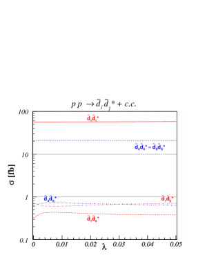
Figure 5.3: Cross sections for charged squark-antisquark (top) and neutral up-type (centre) and down-type (bottom) squark-antisquark pair production at the LHC in our benchmark scenario A.

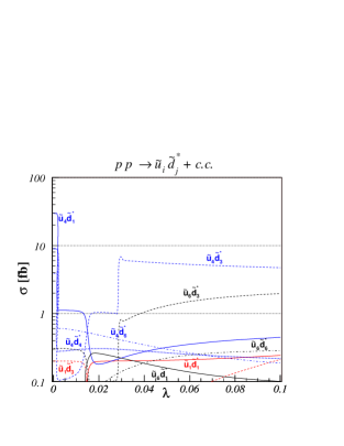
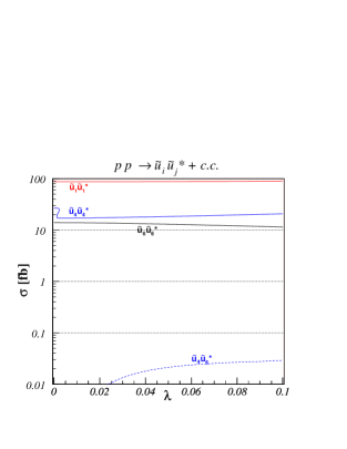
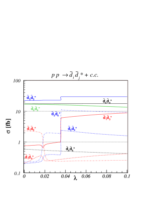
Figure 5.4: Same as Fig. 5.3 for our benchmark scenario B.

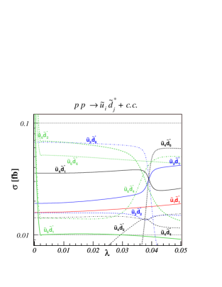
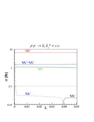
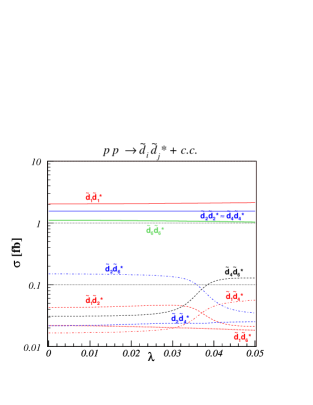
Figure 5.5: Same as Fig. 5.3 for our benchmark scenario C.

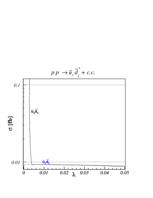
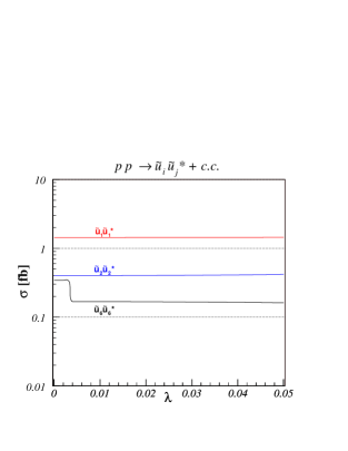
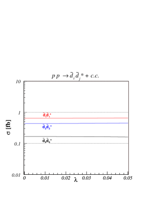
Figure 5.6: Same as Fig. 5.3 for our benchmark scenario D.

We present numerical predictions for the production cross sections of squark-antisquark pairs in NMFV SUSY at the CERN LHC. Again, we use the QCD factorization theorem to compute the total unpolarized hadronic cross sections

$$\sigma \leavevmode\nobreak\ = \int_{4m^{2}/s_{h}}^{1}\!{\rm d}\tau\!\!\int_{-1/2\ln\tau}^{1/2\ln\tau}\!\!{\rm d}y\int_{t_{\min}}^{t_{\max}}{\rm d}t\ f_{a/A}(x_{a},M_{a}^{2})\ f_{b/B}(x_{b},M_{b}^{2})\ {{\rm d}\hat{\sigma}\over{\rm d}t},\leavevmode\nobreak\$$ (5.16)

where the relevant partonic cross section d$\hat{\sigma}$/d$t$ is convolved with universal parton densities. For consistency with our leading order QCD calculation in the collinear approximation, where all squared quark masses, the top excepted, are much lower than the partonic centre-of-mass energy, we employ the LO set of the latest CTEQ6 global parton density fit [222], which includes $n_{f}=5$ “light” quark flavours and the gluon, but no top-quark density. For gluon initial states and gluon or gluino exchanges, the strong coupling constant $\alpha_{s}(\mu_{R})$ is calculated with the corresponding LO value of $\Lambda_{\rm LO}^{n_{f}=5}=165$ MeV. We identify the renormalization scale $\mu_{R}$ with the factorization scales $M_{a}=M_{b}$ and set the scales to the average mass of the final state SUSY particles $i$ and $j$, $m=(m_{i}+m_{j})/2$.

We take current masses and widths of the electroweak gauge bosons, electroweak mixing angle, electromagnetic fine structure constant and CKM matrix elements, while the soft SUSY-breaking masses at the electroweak scale are computed thanks the computer program SPheno 2.2.3 [156]. Then we introduce NMFV as in Sec. 2.3.3 through the parameter $\lambda$ defined in Eq. (2.89). The physical masses of the SUSY particles and the mixing angles, taking into account NMFV, are obtained with the computer program FeynHiggs 2.5.1 [157].

The numerical cross sections for charged squark-antisquark and neutral up- and down-type squark-antisquark pair production are shown in Figs. 5.3, 5.4, 5.5 and 5.6 for the benchmark scenarios A, B, C and D described in Sec. 2.3.3, respectively. The magnitudes of the cross sections vary from the barely visible level of $10^{-2}$ fb for weak production of heavy final states to large cross sections of $10^{2}$ to $10^{3}$ fb for the strong production of diagonal squark-antisquark pairs. Unfortunately, these processes, whose cross sections are largest, are practically insensitive to the flavour violation parameter $\lambda$, as the strong gauge interaction is insensitive to quark flavours.

Some of the subleading, non-diagonal cross sections show, however, sharp transitions, in particular down-type squark-antisquark production at the benchmark point B (bottom panel on Fig. 5.4), but also other squark-antisquark production processes. At $\lambda=0.02$, the cross sections for $\tilde{d}_{1}\tilde{d}_{6}^{\ast}$ and $\tilde{d}_{3}\tilde{d}_{6}^{\ast}$ switch places. The concerned down-type squark mass differences are rather small (see lower right panel of Fig. 2.6), and this flip is then mainly due to the interplay between the different strange and bottom quark densities in the proton and the level reordering phenomenon discussed in Sec. 2.3.4, since at this value of $\lambda$, the flavour contents of $\tilde{d}_{1}$ and $\tilde{d}_{3}$ are exchanged (see Fig. 2.12).

At $\lambda=0.035$, the flavour content of the eigenstate $\tilde{d}_{3}$ switches from $\tilde{s}_{R}$ to $\tilde{d}_{R}$, leading to a sharp increase of the cross sections for $\tilde{d}_{3}\tilde{d}_{6}^{\ast}$ and $\tilde{d}_{1}\tilde{d}_{3}^{\ast}$, since these final states can then be produced from down-type valence quarks. For $\lambda>0.035$, the cross section of the latter process, $\tilde{d}_{1}\tilde{d}_{3}^{\ast}$ production, increases with the strange squark content of $\tilde{d}_{1}$ (see Fig. 2.12). Let us note that all of these non-diagonal squark pair production cross sections are mainly dominated by the exchange of strongly coupled gluinos despite of their large mass.

5.1.3 cMFV limit

We investigate in this subsection the production of diagonal (same mass-eigenstates), non-diagonal (different mass eigenstates) and mixed (different flavours) third generation squark-antisquark pairs within the limit of the constrained Minimal Flavour Violation, where the squark mixing is parameterized only by the two mixing angles $\theta_{\tilde{t}}$ and $\theta_{\tilde{b}}$. The cMFV limit of Eq. (5.13) in the case of diagonal squark-antisquark pair production, keeping only strong contributions and showing explicitly the mixing angle dependence, is given by [96]

$${{\rm d}\hat{\sigma}_{h_{a},h_{b}}^{q\bar{q}}\over{\rm d}t} = {4\pi\alpha_{s}^{2}\over 9s^{2}}\,\left[1-h_{a}h_{b}\right]\,{tu-m_{\tilde{q}}^{4}\over s^{2}}$$ (5.17)

$$- {4\pi\alpha_{s}^{2}\over 27s^{2}}\,\left[1\pm(h_{b}-h_{a})\cos 2\theta_{\tilde{q}}-h_{a}h_{b}\right]\,{tu-m_{\tilde{q}}^{4}\over st_{\tilde{g}}}\,\delta_{qb}\,\delta_{\tilde{q}\tilde{b}}$$

$$+ {\pi\alpha_{s}^{2}\over 18s^{2}}\ \left[{(1\!+\!h_{a}h_{b})\,(1\!-\!\cos 4\theta_{\tilde{q}})\,m_{\tilde{g}}^{2}s\!+\!(1\!-\!h_{a}h_{b})\,(3\!+\!\cos 4\theta_{\tilde{q}})\,(tu\!-\!m_{\tilde{q}}^{4})\over t_{\tilde{g}}^{2}}\right.$$

$$\left.\pm\,4\cos 2\theta_{\tilde{q}}\,(h_{b}-h_{a}){tu-m_{\tilde{q}}^{4}\over t_{\tilde{g}}^{2}}\right]\delta_{qb}\,\delta_{\tilde{q}\tilde{b}},\hskip 113.81102pt$$

where the upper sign holds for $\tilde{b}_{1}$ and the lower sign for $\tilde{b}_{2}$ production. Stops are produced only through $s$-channel gluon exchange due to negligible top quark PDFs in the proton. Even for sbottom production, $t$-channel gluino contributions are suppressed by small bottom PDFs and the heavy gluino propagator. The cross section for the gluon-fusion initiated subprocess in Eq. (5.15) is left unchanged, since it is mixing independent. In the case of no squark mixing, our results agree with the double-polarized and unpolarized cross sections in Ref. [43].

For non-diagonal production, $s$-channel strong diagrams are not present. However, we take into account the PDF-suppressed gluino $t$-channel and the quark-induced tree-level electroweak diagrams, proceeding either through an $s$-channel $Z$-boson exchange or a $t$-channel neutralino exchange,

$${{\rm d}\hat{\sigma}_{h_{a},h_{b}}^{q\bar{q}}\over{\rm d}t} = {\pi\alpha^{2}\over s^{2}}{\sin^{2}(2\theta_{\tilde{q}})\left[(1-h_{a})(1+h_{b})L_{qqZ}^{2}+(1+h_{a})(1-h_{b})R_{qqZ}^{2}\right]\over 32\,x_{W}^{2}\,(1-x_{W})^{2}\,s_{z}^{2}}$$

$$\times\left[tu-m_{\tilde{q}_{1}}^{2}m_{\tilde{q}_{2}}^{2}\right]$$

$$- {\pi\alpha\alpha_{s}\over s^{2}}{\sin^{2}(2\theta_{\tilde{q}})\left[(1-h_{a})(1+h_{b})L_{qqZ}-(1+h_{a})(1-h_{b})R_{qqZ}\right]\over 9\,x_{W}\,(1-x_{W})\,s_{z}\,t_{\tilde{g}}}\ \delta_{qb}\,\delta_{\tilde{q}\tilde{b}}$$

$$\times\left[tu-m_{\tilde{q}_{1}}^{2}m_{\tilde{q}_{2}}^{2}\right]$$

$$+ \ {\pi\alpha_{s}^{2}\over 9s^{2}}\ \left[{\left[(1+h_{a}h_{b})(3+\cos 4\theta_{\tilde{q}})-4(h_{a}+h_{b})\cos 2\theta_{\tilde{q}}\right]m_{\tilde{g}}^{2}s\over t_{\tilde{g}}^{2}}\right.$$

$$\left.+{2\sin^{2}2\theta_{\tilde{q}}(1-h_{a}h_{b})(tu-m_{\tilde{q}_{1}}^{2}m_{\tilde{q}_{2}}^{2})\over t_{\tilde{g}}^{2}}\right]\delta_{qb}\,\delta_{\tilde{q}\tilde{b}}$$

$$- {\pi\alpha^{2}\over s^{2}}\!\sum_{i}\!{\sin^{2}(2\theta_{\tilde{q}})\left[(1\!-\!h_{a})(1\!+\!h_{b})L_{qqZ}L_{\tilde{q}q\tilde{\chi}_{i}^{0}}^{2}\!-\!(1\!+\!h_{a})(1\!-\!h_{b})R_{qqZ}R_{\tilde{q}q\tilde{\chi}_{i}^{0}}^{2}\right]\over 12\,x_{W}^{2}(1\!-\!x_{W})^{2}\,s_{z}\,t_{\tilde{\chi}^{0}_{i}}}$$

$$\times\left[tu-m_{\tilde{q}_{1}}^{2}m_{\tilde{q}_{2}}^{2}\right]\delta_{qb}\,\delta_{\tilde{q}\tilde{b}}$$

$$+ {\pi\alpha^{2}\over s^{2}}\sum_{i,j}\left[{\delta_{qb}\,\delta_{\tilde{q}\tilde{b}}\over(1+\delta_{ij})\,x_{W}^{2}\,(1-x_{W})^{2}\,t_{\tilde{\chi}^{0}_{i}}\,t_{\tilde{\chi}^{0}_{j}}}\right]\Bigg{[}\Big{\{}(1+h_{a}h_{b})(3+\cos 4\theta_{\tilde{q}})$$

$$-4(h_{a}+h_{b})\cos 2\theta_{\tilde{q}}\Big{\}}L_{\tilde{q}q\tilde{\chi}_{i}^{0}}L_{\tilde{q}q\tilde{\chi}_{j}^{0}}R_{\tilde{q}q\tilde{\chi}_{i}^{0}}R_{\tilde{q}q\tilde{\chi}_{j}^{0}}\,m_{\tilde{\chi}^{0}_{i}}m_{\tilde{\chi}^{0}_{j}}s+(tu-m_{\tilde{q}_{1}}^{2}m_{\tilde{q}_{2}}^{2})$$

$$\times\!\sin^{2}2\theta_{\tilde{q}}\Big{\{}\!(\!1\!-\!h_{a}\!)(\!1\!+\!h_{b}\!)L_{\tilde{q}q\tilde{\chi}_{i}^{0}}^{2}L_{\tilde{q}q\tilde{\chi}_{j}^{0}}^{2}\!+\!(1\!+\!h_{a})(1\!-\!h_{b})R_{\tilde{q}q\tilde{\chi}_{i}^{0}}^{2}R_{\tilde{q}q\tilde{\chi}_{j}^{0}}^{2}\!\Big{\}}\!\Bigg{]},\!$$

(5.18)

where we have summed over $\tilde{q}_{1}\tilde{q}_{2}^{\ast}+\tilde{q}_{2}\tilde{q}_{1}^{\ast}$ final states. The coupling strengths

$$L_{\tilde{q}q\tilde{\chi}^{0}_{i}} = \bigg{[}(e_{q}-T^{3}_{q})\,s_{W}N_{i1}+T^{3}_{q}\,c_{W}N_{i2}\bigg{]},\leavevmode\nobreak\$$ (5.19)

$$-R_{\tilde{q}q\tilde{\chi}_{i}^{0}}^{\ast} = e_{q}\,s_{W}\,N_{i1},\leavevmode\nobreak\$$ (5.20)

correspond the the quark-squark-neutralino interactions in the limit of non-mixing left- and right-handed (s)quarks, provided that we neglect the relatively small Yukawa couplings, which is the case here since top (s)quarks do not take part in the considered subprocess.

Finally, mixed squark-pair production, i.e. a pair of one bottom plus one top squark, proceeds at tree-level only through an $s$-channel exchange of a charged $W^{\pm}$-boson, since the $t$-channel exchanges of Fig. 5.1 are PDF-suppressed due to the negligible top density inside the proton. The $\tilde{t}_{1}\tilde{b}_{1}$ production cross section is obtained from Eq. (5.9) by keeping only the $W$ contribution,

$${{\rm d}\hat{\sigma}_{h_{a},h_{b}}^{q\bar{q}^{\prime}}\over{\rm d}t} = {\pi\alpha^{2}\over s^{2}}\ |V_{qq^{\prime}}|^{2}|V_{tb}|^{2}\left[{tu-m_{\tilde{t}_{1}}^{2}m_{\tilde{b}_{1}}^{2}\over s^{2}}\right]{\cos^{2}\theta_{\tilde{t}}\,\cos^{2}\theta_{\tilde{b}}\,(1\!-\!h_{a})(1\!+\!h_{b})\over 4x_{W}^{2}(1-m_{W}^{2}/s)^{2}},\leavevmode\nobreak\ \leavevmode\nobreak\ \leavevmode\nobreak\ \leavevmode\nobreak\ \leavevmode\nobreak\ \leavevmode\nobreak\$$ (5.21)

where we show explicitly the dependence on the CKM matrix elements. For the mixed production of the heavier squark mass eigenstates, the corresponding index 1 has to be replaced by 2 and the squared cosine of the mixing angle by the squared sine.

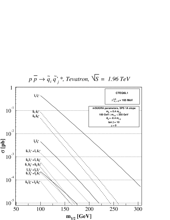
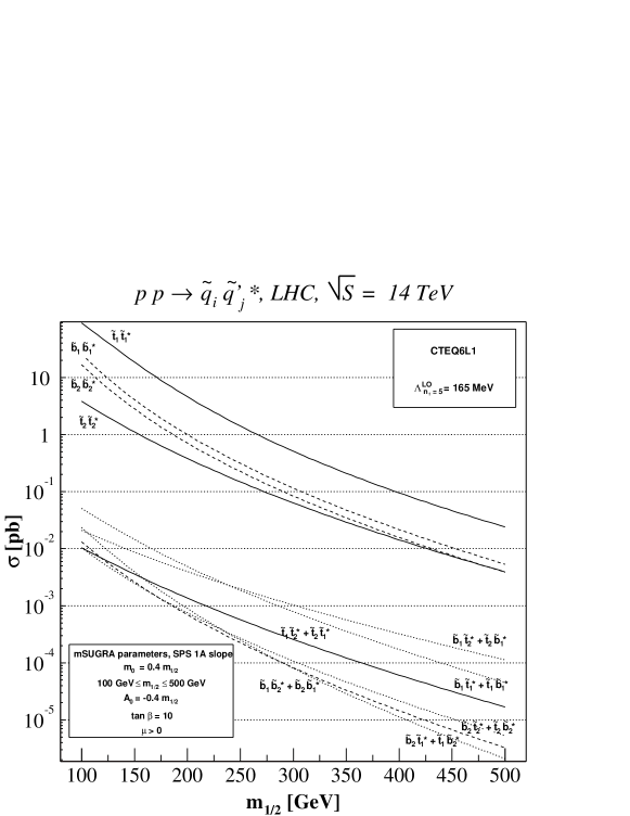
Figure 5.7: Production cross sections for top (full), bottom (dashed), and mixed top and bottom squarks (dotted) at the Tevatron (top figure) and at the LHC (bottom figure) as a function of the common fermion mass $m_{1/2}$ in the mSUGRA model line SPS 1a [45].

In the following, we use older values of the SM parameters [197], and the physical masses of the squarks and mixing matrices are calculated using the computer program SuSpect Version 2.3 [202]. As a first benchmark, we choose the model line SPS 1a [45] described in Sec. 3.3 and show in the top panel of the Fig. 5.7 that cMFV non-diagonal and mixed third generation squark production will be difficult to discover at the Tevatron due to its limited centre-of-mass energy. As one can see, only diagonal production of the lighter top squark mass eigenstate will be visible in the full region of the mSUGRA parameter space shown here with the expected final integrated luminosity of 8.9 fb^-1. For diagonal sbottom production, the accessible parameter space is already reduced to $m_{1/2}\leq 225$ GeV. Non-diagonal and mixed squark production could only be discovered, if the common fermion mass $m_{1/2}$ is not much larger than 100 GeV. As expected for a $p\bar{p}$ collider, the cross sections are very much dominated by $q\bar{q}$ annihilation, even for the diagonal channels, and $gg$ initial states contribute at most 15% in the case of diagonal light stop production.

The LHC with its much larger centre-of-mass energy of and design luminosity of 300 fb^-1 will, in contrast, have no problem in producing all combinations of squarks in sufficient numbers. The hierarchy between the strong diagonal production channels of ${\cal O}(\alpha_{s}^{2})$ and the electroweak non-diagonal and mixed channels of ${\cal O}(\alpha^{2})$ is, however, clearly visible in the bottom panel of Fig. 5.7, the latter being about two orders of magnitude smaller. The LHC being a $pp$ collider and the average $x$-value in the PDFs being considerably smaller, the diagonal channels are enhanced by the high $gg$ luminosity, which dominates their cross sections by up to 93 %. Among the electroweak ${\cal O}(\alpha^{2})$ processes, mixed production of top and bottom squarks is favoured over non-diagonal top or bottom squark production by the possibility of two light masses and a positive charge in the final state, which is more easily produced by the charged $pp$ initial state.

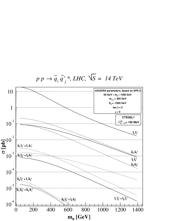
Figure 5.8: Production cross sections for top (full), bottom (dashed), and mixed top and bottom squarks (dotted) at the LHC in the mSUGRA model SPS 5 as a function of the scalar mass $m_{0}$. [45].

We show in Figs. 5.8 numerical results for the LHC, varying $m_{0}$ independently to test the sensitivity of the cross section on the squark masses and mixing, starting from the benchmark point SPS 5 [45], which is a mSUGRA scenario with low $\tan\beta=5$, large $m_{1/2}=350$ GeV, and large negative $A_{0}=-1000$ GeV, leading to heavier sbottoms of 566 and 655 GeV, a heavy $\tilde{t}_{2}$ of 651 GeV, but also a light $\tilde{t}_{1}$ of 259 GeV. We see a clear hierarchy between the dominant pair production of the lighter stop, strong pair production of the heavier stop and sbottoms, charged and neutral electroweak production of final states involving at least one light squark, and finally charged and neutral electroweak production of the heavier squarks, which may only be visible up to $m_{0}\leq 600$ GeV. The more pronounced hierarchy can be explained by the considerable squark mass differences in SPS 5, which lead to additional phase space suppression for the heavier squarks.

5.1.4 QCD one-loop contributions for non-diagonal squark pair production

Within QCD and cMFV SUSY, we have also investigated the possibility to produce non-diagonal squark pairs by the rescattering of diagonal squark pairs through four-squark vertices in the final state, in the limit of a decoupled gluino. The corresponding Feynman diagrams, shown in Fig. 5.9, have one-loop topology and are therefore suppressed by additional squark propagators and/or annihilations within the squark loop. The squared helicity amplitude for the production of non-diagonal stop pairs in gluon-gluon collisions is given by [96]

$$\frac{d\hat{\sigma}_{h_{a},h_{b}}^{gg}}{dt} = (1\!+\!h_{a}h_{b})\left[\frac{37\alpha_{s}^{4}\sin^{2}{\left(4\theta_{\tilde{t}}\right)}}{27648\pi s^{4}}|\Delta\ln_{\tilde{t}}|^{2}\right.\!+\!\sum_{\tilde{q}\neq\tilde{t}}\frac{5\alpha_{s}^{4}\cos^{2}{\left(2\theta_{\tilde{q}}\right)}\sin^{2}{\left(2\theta_{\tilde{t}}\right)}}{3072\pi s^{4}}|\Delta\ln_{\tilde{q}}|^{2}$$ (5.22)

$$+ \sum_{\tilde{q}\neq\tilde{t}}\frac{5\alpha_{s}^{4}\cos{\left(2\theta_{\tilde{q}}\right)}\cos{\left(2\theta_{\tilde{t}}\right)}\sin^{2}{\left(2\theta_{\tilde{t}}\right)}}{2304\pi s^{4}}{\rm Re}\left(\Delta\ln_{\tilde{q}}\Delta\ln_{\tilde{t}}\right)$$

$$+ \!\!\!\left.\!\!\sum_{\tilde{q},\tilde{q}^{\prime}\neq\tilde{t};\tilde{q}\neq\tilde{q}^{\prime}}\frac{5\alpha_{s}^{4}\cos{\left(2\theta_{\tilde{q}}\right)}\cos{\left(2\theta_{\tilde{q}^{\prime}}\right)}\sin^{2}{\left(2\theta_{t}\right)}}{1536\pi s^{4}}{\rm Re}\left(\Delta\ln_{\tilde{q}}\Delta\ln_{\tilde{q^{\prime}}}\right)\right],$$

where

$$\Delta\ln_{\tilde{q}}=m_{\tilde{q}_{1}}^{2}\ln^{2}{\left(-x_{\tilde{q}_{1}}\right)}-m_{\tilde{q}_{2}}^{2}\ln^{2}{\left(-x_{\tilde{q}_{2}}\right)},{\rm\leavevmode\nobreak\ \leavevmode\nobreak\ \leavevmode\nobreak\ \leavevmode\nobreak\ with\leavevmode\nobreak\ \leavevmode\nobreak\ }x_{\tilde{q}_{i}}=\frac{1-\beta_{\tilde{q}_{i}}}{1+\beta_{\tilde{q_{i}}}},\leavevmode\nobreak\$$ (5.23)

and $\beta_{\tilde{q}_{i}}=\sqrt{1-4m_{\tilde{q}_{i}}^{2}}$ is the velocity of the $i^{\rm th}$ squark mass eigenstate. In the limit of degenerate light squarks, only top and bottom squark loops survive loop annihilations, and the squared helicity amplitude simplifies to

$$\frac{d\hat{\sigma}_{h_{a},h_{b}}^{gg}}{dt} = (1+h_{a}h_{b})\left[\frac{37\alpha_{s}^{4}\sin^{2}{\left(4\theta_{\tilde{t}}\right)}}{27648\pi s^{4}}|\Delta\ln_{\tilde{t}}|^{2}\right.+\frac{5\alpha_{s}^{4}\cos^{2}{\left(2\theta_{\tilde{b}}\right)}\sin^{2}{\left(2\theta_{\tilde{t}}\right)}}{3072\pi s^{4}}|\Delta\ln_{\tilde{b}}|^{2}$$ (5.24)

$$+ \left.\frac{5\alpha_{s}^{4}\cos{\left(2\theta_{\tilde{b}}\right)}\cos{\left(2\theta_{\tilde{t}}\right)}\sin^{2}{\left(2\theta_{\tilde{t}}\right)}}{2304\pi s^{4}}{\rm Re}\left(\Delta\ln_{\tilde{b}}\Delta\ln_{\tilde{t}}\right)\right].$$

These expressions have been summed over $\tilde{t}_{1}\tilde{t}_{2}^{\ast}+\tilde{t}_{2}\tilde{t}_{1}^{\ast}$ final states and generalize the corresponding result in Ref. [35], where only top squark loops were taken into account. For non-diagonal sbottom production, top and bottom squark indices have to be exchanged in the equations above.

Figure 5.9: Subdominant loop-level QCD Feynman diagrams for non-diagonal ($i\neq j$) squark production at hadron colliders.

For the non-diagonal third generation squark production $\tilde{t}_{1}\tilde{t}_{2}^{\ast}+\tilde{t}_{2}\tilde{t}_{1}^{\ast}$ and $\tilde{b}_{1}\tilde{b}_{2}^{\ast}+\tilde{b}_{2}\tilde{b}_{1}^{\ast}$, the only contributing diagrams of Fig. 5.2 is the electroweak $Z$-boson exchange, since the QCD $gg$-initiated processes and the gluon $s$-channel are only open for diagonal squark pair production, and the neutralino and gluino diagrams are suppressed by the negligible top and small bottom densities in the proton. Indeed, for the mSUGRA scenario SPS 5, their contributions are found to be six to eight orders of magnitude smaller than the $Z$-contribution. Within the SPS 5 scenario and at the LHC, Fig. 5.11 shows that for non-diagonal stop production, the QCD loop-contributions from Fig. 5.9 are smaller than the electroweak tree-level ones by about one order of magnitude, whereas we naively expect the ${\cal O}(\alpha^{2})$ and ${\cal O}(\alpha_{s}^{4})$ diagrams to contribute with roughly equal strength. As already mentioned, this can be easily explained by the presence of additional heavy squark propagators in the loop diagrams. Here, we consider not only loops involving top, but also bottom squarks, which do not cancel in Eq. (5.24), if the masses of the two bottom squarks are unequal. However, the non-diagonal elements in the squark mass matrices are proportional to the relevant SM quark mass and $m_{b}\ll m_{t}$, so that mixing effects are less important for sbottoms than for stops. Consequently, sbottom loops contribute about one order of magnitude less than stop loops, as can also be seen in Fig. 5.11. SUSY-QCD loop diagrams involving gluino exchanges have not been calculated here, as they are of ${\cal O}(\alpha_{s}^{4})$ and require in addition the presence of heavy top quark and gluino propagators in the loop. In the SPS 5 scenario, we have indeed a heavy gluino of mass $m_{\tilde{g}}=725$ GeV. The dependence on the cosine of the stop mixing angle in the electroweak cross section of Eq. (5.21) and in the the sbottom loop contribution in Eq. (5.24) through $\sin^{2}(2\theta_{\tilde{t}})=4\cos^{2}\theta_{\tilde{t}}\leavevmode\nobreak\ (1-\cos^{2}\theta_{\tilde{t}})$ is clearly visible in Fig. 5.11. In contrast, the stop loop contribution in Eq. (5.24) has a steeper dependence through $\sin^{2}(4\theta_{\tilde{t}})=16\cos^{2}\theta_{\tilde{t}}\leavevmode\nobreak\ (1-\cos^{2}\theta_{\tilde{t}})\leavevmode\nobreak\ (1-2\cos^{2}\theta_{\tilde{t}})^{2}$, which is also visible in the figure.

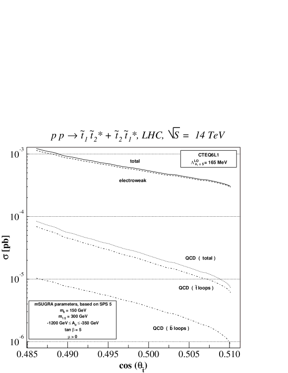
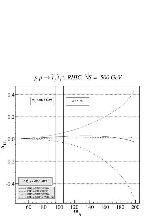
Figure 5.10: Contributions of tree-level electroweak and loop-level QCD processes to non-diagonal stop production at the LHC in the mSUGRA model SPS 5 [45] with a light top squark as a function of the cosine of the top squark mixing angle, together with their sums.

Figure 5.11: Contributions of the $q\bar{q}$ (dotted) and $gg$ (dot-dashed) initial states to the longitudinal double-spin asymmetry $A_{LL}$ at RHIC, together with their sum (full), for stop pair production as a function of the light top squark mass. The total asymmetry using GRSV-VAL (dashed) instead of GRSV-STD (full) parton densities [201] is also shown.

5.1.5 Double-spin asymmetries

As a possible application of the polarization dependence of our analytical results, we show in Fig. 5.11 the double-spin asymmetry of diagonal light stop production at RHIC (within cMFV SUSY). As this polarized $pp$ collider has only a rather small centre-of-mass energy of $\sqrt{s_{h}}=500$ GeV, the observable stop mass range is obviously very limited. Already for $m_{\tilde{t}_{1}}>106$ GeV, the unpolarized cross section drops below 1 fb, while stop masses below 96 GeV are most likely already excluded [149]. This leaves only a very small mass window of 10 GeV for possible observations. In Fig. 5.11 one can clearly see the rise of the asymmetry for $q\bar{q}$ and $gg$ initial states, as the stop mass and the correlated $x$-value in the PDFs grows. However, as the two asymmetries are approximately of equal size, but opposite sign, the total observable asymmetry rests below the 5% level in the entire mass range shown. This is true for both choices of polarized parton densities, GRSV 2000 standard (STD) as well as valence (VAL) [201]. For consistency, the unpolarized cross sections have been calculated in this case using the GRV 98 parton density set [200], as in Sec. 4.1.

5.2 NMFV squark pair production

5.2.1 Analytical results

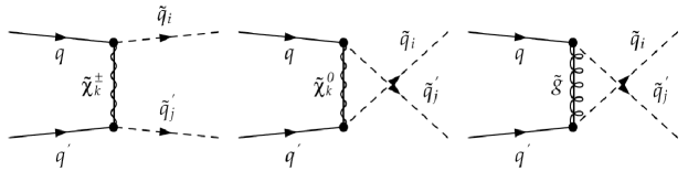
Figure 5.12: Tree-level Feynman diagrams for the production of one down-type squark ($\tilde{q}_{i}$) and one up-type squark ($\tilde{q}_{j}^{\prime}$) in the collision of an up-type quark ($q$) and a down-type quark ($q^{\prime}$).

While squark-antisquark pairs are readily produced in $p\bar{p}$ collisions, e.g. at the Tevatron, from valence quarks and antiquarks, $pp$ colliders have a larger quark-quark luminosity and will thus more easily lead to squark pair production. The potentially flavour-violating production of one down-type and one up-type squark

$$q(h_{a},p_{a})\,q^{\prime}(h_{b},p_{b})\to\tilde{d}_{i}(p_{1})\,\tilde{u}_{j}(p_{2}),$$ (5.25)

in the collision of an up-type quark $q$ and a down-type quark $q^{\prime}$ proceeds through the $t$-channel chargino or $u$-channel neutralino and gluino exchanges shown in Fig. 5.12. The corresponding cross section within NMFV SUSY [97]

$$\frac{d\hat{\sigma}^{qq^{\prime}}_{h_{a},h_{b}}}{dt} = (1\!-\!h_{a})(1\!-\!h_{b})\Bigg{[}\bigg{(}\sum_{k=1,2\atop l=1,2}\!\frac{\mathcal{C}^{kl}_{11}}{t_{\tilde{\chi}_{k}}\,t_{\tilde{\chi}_{l}}}\bigg{)}\!+\!\bigg{(}\sum_{k=1,\ldots,4\atop l=1,\ldots,4}\!\frac{\mathcal{N}_{11}^{kl}}{u_{\tilde{\chi}_{k}^{0}}\,u_{\tilde{\chi}_{l}^{0}}}\bigg{)}\!+\!\frac{\mathcal{G}_{11}}{u_{\tilde{g}}^{2}}$$ (5.26)

$$\!+\! \bigg{(}\sum_{k=1,2\atop l=1,\ldots,4}\!\frac{\mathcal{[CN]}^{kl}_{11}}{t_{\tilde{\chi}_{k}}\,u_{\tilde{\chi}_{l}^{0}}}\bigg{)}+\bigg{(}\sum_{k=1,2}\!\frac{\mathcal{[CG]}^{k}_{11}}{t_{\tilde{\chi}_{k}}\,u_{\tilde{g}}}\bigg{)}\Bigg{]}\!+\!(1\!+\!h_{a})(1\!+\!h_{b})\Bigg{[}\bigg{(}\sum_{k=1,2\atop l=1,2}\!\frac{\mathcal{C}^{kl}_{22}}{t_{\tilde{\chi}_{k}}\,t_{\tilde{\chi}_{l}}}\bigg{)}$$

$$\!+\! \bigg{(}\sum_{k=1,\ldots,4\atop l=1,\ldots,4}\!\frac{\mathcal{N}_{22}^{kl}}{u_{\tilde{\chi}_{k}^{0}}\,u_{\tilde{\chi}_{l}^{0}}}\bigg{)}\!+\!\frac{\mathcal{G}_{22}}{u_{\tilde{g}}^{2}}+\bigg{(}\sum_{k=1,2\atop l=1,\ldots,4}\!\frac{\mathcal{[CN]}^{kl}_{22}}{t_{\tilde{\chi}_{k}}\,u_{\tilde{\chi}_{l}^{0}}}\bigg{)}\!+\!\bigg{(}\sum_{k=1,2}\!\frac{\mathcal{[CG]}^{k}_{22}}{t_{\tilde{\chi}_{k}}\,u_{\tilde{g}}}\bigg{)}\Bigg{]}$$

$$\!+\! (1\!-\!h_{a})(1\!+\!h_{b})\Bigg{[}\bigg{(}\sum_{k=1,2\atop l=1,2}\!\frac{\mathcal{C}^{kl}_{12}}{t_{\tilde{\chi}_{k}}\,t_{\tilde{\chi}_{l}}}\bigg{)}\!+\!\bigg{(}\sum_{k=1,\ldots,4\atop l=1,\ldots,4}\!\frac{\mathcal{N}_{12}^{kl}}{u_{\tilde{\chi}_{k}^{0}}\,u_{\tilde{\chi}_{l}^{0}}}\bigg{)}\!+\!\frac{\mathcal{G}_{12}}{u_{\tilde{g}}^{2}}$$

$$\!+\! \bigg{(}\sum_{k=1,2\atop l=1,\ldots,4}\!\frac{\mathcal{[CN]}^{kl}_{12}}{t_{\tilde{\chi}_{k}}\,u_{\tilde{\chi}_{l}^{0}}}\bigg{)}\!+\!\bigg{(}\sum_{k=1,2}\!\frac{\mathcal{[CG]}^{k}_{12}}{t_{\tilde{\chi}_{k}}\,u_{\tilde{g}}}\bigg{)}\Bigg{]}\!+\!(1\!+\!h_{a})(1\!-\!h_{b})\Bigg{[}\bigg{(}\sum_{k=1,2\atop l=1,2}\!\frac{\mathcal{C}^{kl}_{21}}{t_{\tilde{\chi}_{k}}\,t_{\tilde{\chi}_{l}}}\bigg{)}$$

$$\!+\! \bigg{(}\sum_{k=1,\ldots,4\atop l=1,\ldots,4}\!\frac{\mathcal{N}_{21}^{kl}}{u_{\tilde{\chi}_{k}^{0}}\,u_{\tilde{\chi}_{l}^{0}}}\bigg{)}\!+\!\frac{\mathcal{G}_{21}}{u_{\tilde{g}}^{2}}\!+\!\bigg{(}\sum_{k=1,2\atop l=1,\ldots,4}\!\frac{\mathcal{[CN]}^{kl}_{21}}{t_{\tilde{\chi}_{k}}\,u_{\tilde{\chi}_{l}^{0}}}\bigg{)}\!+\!\bigg{(}\sum_{k=1,2}\!\frac{\mathcal{[CG]}^{k}_{21}}{t_{\tilde{\chi}_{k}}\,u_{\tilde{g}}}\bigg{)}\Bigg{]}\leavevmode\nobreak\ \leavevmode\nobreak\$$

involves the form factors

$$\mathcal{C}_{mn}^{kl} = \frac{\pi\,\alpha^{2}}{4\,x_{W}^{2}\,s^{2}}\mathcal{C}^{n}_{\tilde{u}_{j}q^{\prime}\tilde{\chi}_{k}^{\pm}}\,\mathcal{C}^{m\ast}_{\tilde{d}_{i}q\tilde{\chi}_{k}^{\pm}}\,\mathcal{C}^{n\ast}_{\tilde{u}_{j}q^{\prime}\tilde{\chi}_{l}^{\pm}}\,\mathcal{C}^{m}_{\tilde{d}_{i}q\tilde{\chi}_{l}^{\pm}}\,\Bigg{[}\left(u\,t-m^{2}_{\tilde{d}_{i}}\,m^{2}_{\tilde{u}_{j}}\right)\left(1-\delta_{mn}\right)$$

$$+m_{\tilde{\chi}^{\pm}_{k}}\,\,m_{\tilde{\chi}^{\pm}_{l}}\,s\,\delta_{mn}\Bigg{]},\leavevmode\nobreak\$$

$$\mathcal{N}_{mn}^{kl} = \frac{\pi\,\alpha^{2}}{x_{W}^{2}(1\!-\!x_{W})^{2}s^{2}}\mathcal{C}^{m\ast}_{\tilde{u}_{j}q\tilde{\chi}_{k}^{0}}\mathcal{C}^{n\ast}_{\tilde{d}_{i}q^{\prime}\tilde{\chi}_{k}^{0}}\mathcal{C}^{m}_{\tilde{u}_{j}q\tilde{\chi}_{l}^{0}}\mathcal{C}^{n}_{\tilde{d}_{i}q^{\prime}\tilde{\chi}_{l}^{0}}\Bigg{[}\left(u\,t\!-\!m^{2}_{\tilde{d}_{i}}\,m^{2}_{\tilde{u}_{j}}\right)\left(1\!-\!\delta_{mn}\right)$$

$$+m_{\tilde{\chi}^{0}_{k}}\,m_{\tilde{\chi}^{0}_{l}}\,s\,\delta_{mn}\Bigg{]},\leavevmode\nobreak\$$

$$\mathcal{G}_{mn} = \frac{2\,\pi\,\alpha_{s}^{2}}{9\,s^{2}}\left|\mathcal{C}^{m}_{\tilde{u}_{j}q\tilde{g}}\,\mathcal{C}^{n}_{\tilde{d}_{i}q^{\prime}\tilde{g}}\right|^{2}\Bigg{[}\left(u\,t-m^{2}_{\tilde{d}_{i}}\,m^{2}_{\tilde{u}_{j}}\right)\left(1-\delta_{mn}\right)+m_{\tilde{g}}^{2}\,s\,\delta_{mn}\Bigg{]},\leavevmode\nobreak\$$

$$\mathcal{[CN]}^{kl}_{mn} = \frac{\pi\,\alpha^{2}}{3\,x_{W}^{2}\,(1-x_{W})\,s^{2}}{\rm Re}\left[\mathcal{C}^{n}_{\tilde{u}_{j}q^{\prime}\tilde{\chi}_{k}^{\pm}}\,\mathcal{C}^{m\ast}_{\tilde{d}_{i}q\tilde{\chi}_{k}^{\pm}}\,\mathcal{C}^{m}_{\tilde{u}_{j}q\tilde{\chi}_{l}^{0}}\,\mathcal{C}^{n}_{\tilde{d}_{i}q^{\prime}\tilde{\chi}_{l}^{0}}\right]$$

$$\times\Bigg{[}\left(u\,t-m^{2}_{\tilde{d}_{i}}\,m^{2}_{\tilde{u}_{j}}\right)\left(\delta_{mn}-1\right)+m_{\tilde{\chi}^{\pm}_{k}}\,m_{\tilde{\chi}^{0}_{l}}\,s\,\delta_{mn}\Bigg{]},\leavevmode\nobreak\ \leavevmode\nobreak\$$

$$\mathcal{[CG]}^{k}_{mn} = \frac{4\,\pi\,\alpha\,\alpha_{s}}{9\,s^{2}\,x_{W}}{\rm Re}\left[\mathcal{C}^{n}_{\tilde{u}_{j}q^{\prime}\tilde{\chi}_{k}^{\pm}}\,\mathcal{C}^{m\ast}_{\tilde{d}_{i}q\tilde{\chi}_{k}^{\pm}}\,\mathcal{C}^{m\ast}_{\tilde{u}_{j}q\tilde{g}}\,\mathcal{C}^{n\ast}_{\tilde{d}_{i}q^{\prime}\tilde{g}}\right]\Bigg{[}\left(u\,t-m^{2}_{\tilde{d}_{i}}\,m^{2}_{\tilde{u}_{j}}\right)\left(\delta_{mn}-1\right)$$ (5.27)

$$+m_{\tilde{\chi}^{\pm}_{k}}\,m_{\tilde{g}}\,s\,\delta_{mn}\Bigg{]},$$

where the neutralino-gluino interference term is absent due to colour conservation. The cross section for the charge-conjugate production of antisquarks from antiquarks can be obtained from the equations above by replacing $h_{a,b}\to-h_{a,b}$. Heavy-flavour final states are completely absent in cMFV due to the negligible top quark and small bottom quark densities in the proton and can thus only be obtained in NMFV.

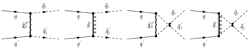
Figure 5.13: Tree-level Feynman diagrams for the production of two up-type or down-type squarks.

The Feynman diagrams for pair production of two up- or down-type squarks with non-minimal flavour violation

$$q(h_{a},p_{a})\,q^{\prime}(h_{b},p_{b}) \to \tilde{q}_{i}(p_{1})\,\tilde{q}_{j}(p_{2})$$ (5.28)

are shown in Fig. 5.13. In NMFV SUSY, neutralino and gluino exchanges can lead to identical squark flavours for different quark initial states, so that both $t$- and $u$-channels contribute and may interfere. The cross section [97]

$$\frac{d\hat{\sigma}^{qq^{\prime}}_{h_{a},h_{b}}}{dt} = (1-h_{a})(1-h_{b})\Bigg{[}\bigg{(}\sum_{k=1,\ldots,4\atop l=1,\ldots,4}\frac{[\mathcal{NT}]_{11}^{kl}}{t_{\tilde{\chi}_{k}^{0}}\,t_{\tilde{\chi}_{l}^{0}}}+\frac{[\mathcal{NU}]_{11}^{kl}}{u_{\tilde{\chi}_{k}^{0}}\,u_{\tilde{\chi}_{l}^{0}}}+\frac{[\mathcal{NTU}]_{11}^{kl}}{t_{\tilde{\chi}_{k}^{0}}\,u_{\tilde{\chi}_{l}^{0}}}\bigg{)}+\frac{[\mathcal{GT}]_{11}}{t_{\tilde{g}}^{2}}$$ (5.29)

$$+ \frac{[\mathcal{GU}]_{11}}{u_{\tilde{g}}^{2}}+\frac{[\mathcal{GTU]}_{11}}{u_{\tilde{g}}t_{\tilde{g}}}+\bigg{(}\sum_{k=1,\ldots,4}\frac{[\mathcal{NGA}]_{11}^{k}}{t_{\tilde{\chi}_{k}^{0}}\,u_{\tilde{g}}}+\frac{[\mathcal{NGB}]_{11}^{k}}{u_{\tilde{\chi}_{k}^{0}}\,t_{\tilde{g}}}\bigg{)}\Bigg{]}\frac{1}{1+\delta_{ij}}$$

$$+ (1+h_{a})(1+h_{b})\Bigg{[}\bigg{(}\sum_{k=1,\ldots,4\atop l=1,\ldots,4}\frac{[\mathcal{NT}]_{22}^{kl}}{t_{\tilde{\chi}_{k}^{0}}\,t_{\tilde{\chi}_{l}^{0}}}+\frac{[\mathcal{NU}]_{22}^{kl}}{u_{\tilde{\chi}_{k}^{0}}\,u_{\tilde{\chi}_{l}^{0}}}+\frac{[\mathcal{NTU}]_{22}^{kl}}{t_{\tilde{\chi}_{k}^{0}}\,u_{\tilde{\chi}_{l}^{0}}}\bigg{)}+\frac{[\mathcal{GT]}_{22}}{t_{\tilde{g}}^{2}}$$

$$+ \frac{[\mathcal{GU]}_{22}}{u_{\tilde{g}}^{2}}+\frac{[\mathcal{GTU]}_{22}}{u_{\tilde{g}}t_{\tilde{g}}}+\bigg{(}\sum_{k=1,\ldots,4}\frac{[\mathcal{NGA}]_{22}^{k}}{t_{\tilde{\chi}_{k}^{0}}\,u_{\tilde{g}}}+\frac{[\mathcal{NGB}]_{22}^{k}}{u_{\tilde{\chi}_{k}^{0}}\,t_{\tilde{g}}}\bigg{)}\Bigg{]}\frac{1}{1+\delta_{ij}}$$

$$+ (1-h_{a})(1+h_{b})\Bigg{[}\bigg{(}\sum_{k=1,\ldots,4\atop l=1,\ldots,4}\frac{[\mathcal{NT}]_{12}^{kl}}{t_{\tilde{\chi}_{k}^{0}}\,t_{\tilde{\chi}_{l}^{0}}}+\frac{[\mathcal{NU}]_{12}^{kl}}{u_{\tilde{\chi}_{k}^{0}}\,u_{\tilde{\chi}_{l}^{0}}}+\frac{[\mathcal{NTU}]_{12}^{kl}}{t_{\tilde{\chi}_{k}^{0}}\,u_{\tilde{\chi}_{l}^{0}}}\bigg{)}+\frac{[\mathcal{GT]}_{12}}{t_{\tilde{g}}^{2}}$$

$$+ \frac{[\mathcal{GU]}_{12}}{u_{\tilde{g}}^{2}}+\frac{[\mathcal{GTU]}_{12}}{u_{\tilde{g}}t_{\tilde{g}}}+\bigg{(}\sum_{k=1,\ldots,4}\frac{[\mathcal{NGA}]_{12}^{k}}{t_{\tilde{\chi}_{k}^{0}}\,u_{\tilde{g}}}+\frac{[\mathcal{NGB}]_{12}^{k}}{u_{\tilde{\chi}_{k}^{0}}\,t_{\tilde{g}}}\bigg{)}\Bigg{]}\frac{1}{1+\delta_{ij}}$$

$$+ (1+h_{a})(1-h_{b})\Bigg{[}\bigg{(}\sum_{k=1,\ldots,4\atop l=1,\ldots,4}\frac{[\mathcal{NT}]_{21}^{kl}}{t_{\tilde{\chi}_{k}^{0}}\,t_{\tilde{\chi}_{l}^{0}}}+\frac{[\mathcal{NU}]_{21}^{kl}}{u_{\tilde{\chi}_{k}^{0}}\,u_{\tilde{\chi}_{l}^{0}}}+\frac{[\mathcal{NTU}]_{21}^{kl}}{t_{\tilde{\chi}_{k}^{0}}\,u_{\tilde{\chi}_{l}^{0}}}\bigg{)}+\frac{[\mathcal{GT]}_{21}}{t_{\tilde{g}}^{2}}$$

$$+ \frac{[\mathcal{GU]}_{21}}{u_{\tilde{g}}^{2}}+\frac{[\mathcal{GTU]}_{21}}{u_{\tilde{g}}t_{\tilde{g}}}+\bigg{(}\sum_{k=1,\ldots,4}\frac{[\mathcal{NGA}]_{21}^{k}}{t_{\tilde{\chi}_{k}^{0}}\,u_{\tilde{g}}}+\frac{[\mathcal{NGB}]_{21}^{k}}{u_{\tilde{\chi}_{k}^{0}}\,t_{\tilde{g}}}\bigg{)}\Bigg{]}\frac{1}{1+\delta_{ij}}$$

depends therefore on the form factors

$$[\mathcal{NT}]_{mn}^{kl} = \frac{\pi\,\alpha^{2}}{x_{W}^{2}\,(1-x_{W})^{2}\,s^{2}}\mathcal{C}^{n\ast}_{\tilde{q}_{j}q^{\prime}\tilde{\chi}_{k}^{0}}\,\mathcal{C}^{m\ast}_{\tilde{q}_{i}q\tilde{\chi}_{k}^{0}}\,\mathcal{C}^{n}_{\tilde{q}_{j}q^{\prime}\tilde{\chi}_{l}^{0}}\,\mathcal{C}^{m}_{\tilde{q}_{i}q\tilde{\chi}_{l}^{0}}\,\Bigg{[}\left(u\,t-m^{2}_{\tilde{q}_{i}}\,m^{2}_{\tilde{q}_{j}}\right)$$

$$\times\left(1-\delta_{mn}\right)+m_{\tilde{\chi}^{0}_{k}}\,m_{\tilde{\chi}^{0}_{l}}\,s\,\delta_{mn}\Bigg{]},\leavevmode\nobreak\$$

$$\large[\mathcal{NU}\large]_{mn}^{kl} = \frac{\pi\,\alpha^{2}}{x_{W}^{2}\,(1-x_{W})^{2}\,s^{2}}\mathcal{C}^{n\ast}_{\tilde{q}_{i}q^{\prime}\tilde{\chi}_{k}^{0}}\,\mathcal{C}^{m\ast}_{\tilde{q}_{j}q\tilde{\chi}_{k}^{0}}\,\mathcal{C}^{n}_{\tilde{q}_{i}q^{\prime}\tilde{\chi}_{l}^{0}}\,\mathcal{C}^{m}_{\tilde{q}_{j}q\tilde{\chi}_{l}^{0}}\,\Bigg{[}\left(u\,t-m^{2}_{\tilde{q}_{i}}\,m^{2}_{\tilde{q}_{j}}\right)$$

$$\times\left(1-\delta_{mn}\right)+m_{\tilde{\chi}^{0}_{k}}\,m_{\tilde{\chi}^{0}_{l}}\,s\,\delta_{mn}\Bigg{]},\leavevmode\nobreak\$$

$$\large[\mathcal{NTU}\large]_{mn}^{kl} = \frac{2\,\pi\,\alpha^{2}}{3\,x_{W}^{2}\,(1-x_{W})^{2}\,s^{2}}{\rm Re}\left[\mathcal{C}^{m\ast}_{\tilde{q}_{i}q\tilde{\chi}_{k}^{0}}\,\mathcal{C}^{n\ast}_{\tilde{q}_{j}q^{\prime}\tilde{\chi}_{k}^{0}}\,\mathcal{C}^{n}_{\tilde{q}_{i}q^{\prime}\tilde{\chi}_{l}^{0}}\,\mathcal{C}^{m}_{\tilde{q}_{j}q\tilde{\chi}_{l}^{0}}\right]$$

$$\times\Bigg{[}\left(u\,t-m^{2}_{\tilde{q}_{i}}\,m^{2}_{\tilde{q}_{j}}\right)\left(1-\delta_{mn}\right)+m_{\tilde{\chi}^{0}_{k}}\,m_{\tilde{\chi}^{0}_{l}}\,s\,\delta_{mn}\Bigg{]},\leavevmode\nobreak\$$

$$\large[\mathcal{GT}\large]_{mn} = \frac{2\,\pi\,\alpha_{s}^{2}}{9\,s^{2}}\left|\mathcal{C}^{n}_{\tilde{q}_{j}q^{\prime}\tilde{g}}\,\mathcal{C}^{m}_{\tilde{q}_{i}q\tilde{g}}\right|^{2}\Bigg{[}\left(u\,t-m^{2}_{\tilde{q}_{i}}\,m^{2}_{\tilde{q}_{j}}\right)\left(1-\delta_{mn}\right)+m_{\tilde{g}}^{2}\,s\,\delta_{mn}\Bigg{]},\leavevmode\nobreak\$$

$$\large[\mathcal{GU}\large]_{mn} = \frac{2\,\pi\,\alpha_{s}^{2}}{9\,s^{2}}\left|\mathcal{C}^{m}_{\tilde{q}_{i}q^{\prime}\tilde{g}}\,\mathcal{C}^{n}_{\tilde{q}_{j}q\tilde{g}}\right|^{2}\Bigg{[}\left(u\,t-m^{2}_{\tilde{q}_{i}}\,m^{2}_{\tilde{q}_{j}}\right)\left(1-\delta_{mn}\right)+m_{\tilde{g}}^{2}\,s\,\delta_{mn}\Bigg{]},\leavevmode\nobreak\$$

$$\large[\mathcal{GTU}\large]_{mn} = \frac{-4\,\pi\,\alpha_{s}^{2}}{27\,s^{2}}{\rm Re}\left[\mathcal{C}^{m}_{\tilde{q}_{i}q\tilde{g}}\,\mathcal{C}^{n}_{\tilde{q}_{j}q^{\prime}\tilde{g}}\mathcal{C}^{m\ast}_{\tilde{q}_{i}q^{\prime}\tilde{g}}\,\mathcal{C}^{n\ast}_{\tilde{q}_{j}q\tilde{g}}\right]\Bigg{[}\left(u\,t-m^{2}_{\tilde{q}_{i}}\,m^{2}_{\tilde{q}_{j}}\right)\left(1-\delta_{mn}\right)$$

$$+m_{\tilde{g}}^{2}\,s\,\delta_{mn}\Bigg{]},\leavevmode\nobreak\$$

$$\large[\mathcal{NGA}\large]_{mn}^{k} = \frac{8\,\pi\,\alpha\alpha_{s}}{9\,s^{2}\,x_{W}\,(1-x_{W})}{\rm Re}\left[\mathcal{C}^{n\ast}_{\tilde{q}_{j}q^{\prime}\tilde{\chi}_{k}^{0}}\,\mathcal{C}^{m\ast}_{\tilde{q}_{i}q\tilde{\chi}_{k}^{0}}\,\mathcal{C}^{m\ast}_{\tilde{q}_{i}q^{\prime}\tilde{g}}\,\mathcal{C}^{n\ast}_{\tilde{q}_{j}q\tilde{g}}\right]\Bigg{[}\left(u\,t-m^{2}_{\tilde{q}_{i}}\,m^{2}_{\tilde{q}_{j}}\right)$$

$$\times\left(1-\delta_{mn}\right)+m_{\tilde{\chi}^{0}_{k}}\,m_{\tilde{g}}\,s\,\delta_{mn}\Bigg{]},\leavevmode\nobreak\$$

$$\large[\mathcal{NGB}\large]_{mn}^{k} = \frac{8\,\pi\,\alpha\alpha_{s}}{9\,s^{2}\,x_{W}\,(1-x_{W})}{\rm Re}\left[\mathcal{C}^{n\ast}_{\tilde{q}_{i}q^{\prime}\tilde{\chi}_{k}^{0}}\,\mathcal{C}^{m\ast}_{\tilde{q}_{j}q\tilde{\chi}_{k}^{0}}\,\mathcal{C}^{n\ast}_{\tilde{q}_{j}q^{\prime}\tilde{g}}\,\mathcal{C}^{m\ast}_{\tilde{q}_{i}q\tilde{g}}\right]\Bigg{[}\left(u\,t-m^{2}_{\tilde{q}_{i}}\,m^{2}_{\tilde{q}_{j}}\right)$$ (5.30)

$$\times\left(1-\delta_{mn}\right)+m_{\tilde{\chi}^{0}_{k}}\,m_{\tilde{g}}\,s\,\delta_{mn}\Bigg{]}.$$

Gluinos will dominate over neutralino exchanges due to their strong coupling, and the two will only interfere in the mixed $t$- and $u$-channels due to colour conservation. At the LHC, up-type squark pair production should dominate over mixed up-/down-type squark production and down-type squark pair production, since the proton contains two valence up-quarks and only one valence down-quark. As before, the charge-conjugate production of antisquark pairs is obtained by making the replacement $h_{a,b}\to-h_{a,b}$. If we neglect electroweak contributions as well as squark flavour and helicity mixing and sum over left- and right-handed squark states, our results agree with those of Ref. [31].

5.2.2 Numerical results

As in Sec. 5.1.2, we employ the LO set of the latest CTEQ6 global parton density fit [222], with five active flavours and the gluon, and the strong coupling constant is calculated with the value of $\Lambda_{\rm LO}^{n_{f}=5}=165$ MeV. The renormalization and factorization scales are set to the average mass of the final state SUSY particles, and the SUSY masses and mixings are again computed with the help of SPheno and FeynHiggs.

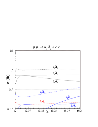
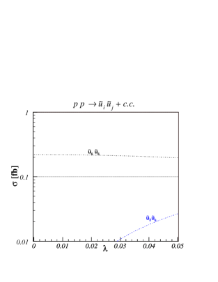
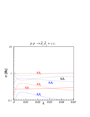
Figure 5.14: Cross sections for mixed (top), up-type (centre) and down-type (bottom) squark-squark pair production at the LHC in our benchmark scenario A.

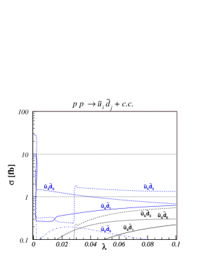
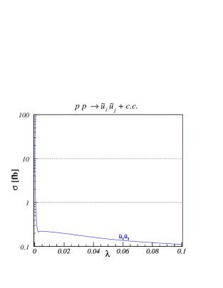
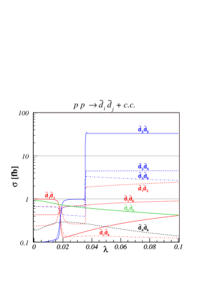
Figure 5.15: Same as Fig. 5.14 for our benchmark scenario B.

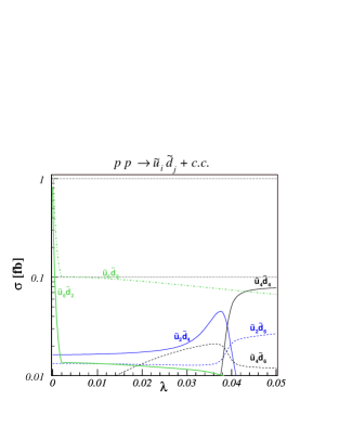
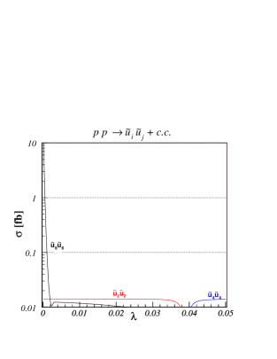
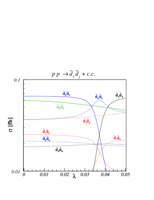
Figure 5.16: Same as Fig. 5.14 for our benchmark scenario C.

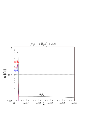
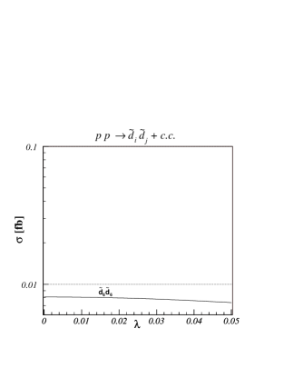
Figure 5.17: Same as Fig. 5.14 for our benchmark scenario D.

The numerical cross sections for mixed, up- and down-type squark-squark pair production are shown in Figs. 5.14, 5.15, 5.16 and 5.17 for the benchmark scenarios A, B, C and D described in Sec. 2.3.3, respectively, where we show their dependence on the flavour violating parameter $\lambda$ (see Eq. (2.89)). While the diagonal channels are practically insensitive to flavour violation, some of the non-diagonal cross sections show sharp transitions, as for example at the benchmark point C (Fig. 5.16) where they occur between the $\tilde{u}_{2}/\tilde{u}_{4}$ and $\tilde{d}_{2}/\tilde{d}_{4}$ states, which are pure charm/strange squarks below/above $\lambda=0.035$. As a side-remark we note that an interesting perspective might be the exploitation of these $t$-channel contributions to second- and third-generation squark production for the determination of heavy-quark densities in the proton. This requires, of course, efficient experimental techniques for heavy-flavour tagging.

5.3 NMFV associated production of squarks and gauginos

5.3.1 Analytical results

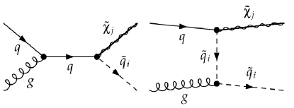
Figure 5.18: Tree-level Feynman diagrams for the associated production of squarks and gauginos.

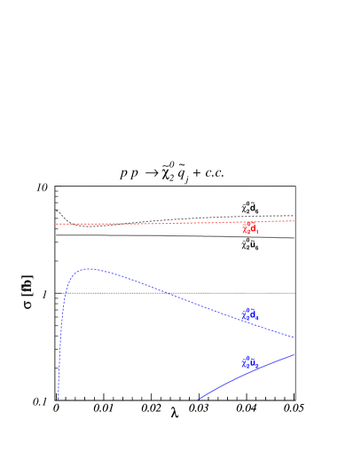
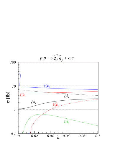
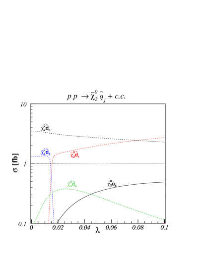
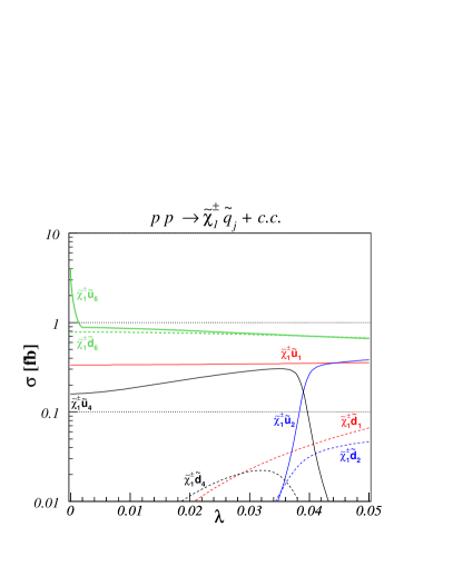
Figure 5.19: Cross sections for associated production of squarks with charginos (left) and neutralinos (right) at the LHC in our benchmark scenario A.

Figure 5.20: Same as Fig. 5.20 for our benchmark scenario B.

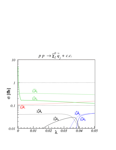
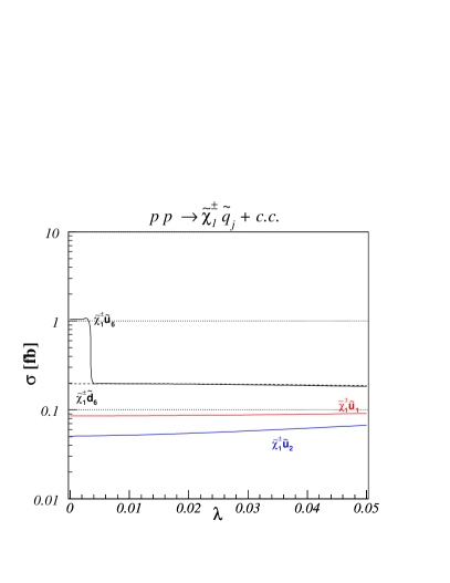
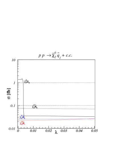
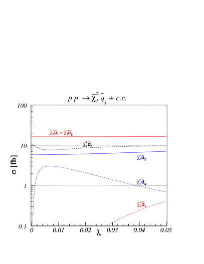
Figure 5.21: Same as Fig. 5.20 for our benchmark scenario C.

Figure 5.22: Same as Fig. 5.20 for our benchmark scenario D.

The associated production of squarks and neutralinos or charginos

$$q(h_{a},p_{a})\,g(h_{b},p_{b})\to\tilde{\chi}_{j}(p_{1})\,\tilde{q}_{i}(p_{2})$$ (5.31)

is a semi-weak process that originates from quark-gluon initial states and has both an $s$-channel quark and a $t$-channel squark contribution. They involve both a quark-squark-gaugino vertex that can in general be flavour violating. The corresponding Feynman diagrams can be seen in Fig. 5.18. The squark-gaugino cross section is given by [97]

$$\frac{d\hat{\sigma}^{qg}_{h_{a},h_{b}}}{dt} = \frac{\pi\,\alpha\,\alpha_{s}}{n_{\tilde{\chi}}\,s^{2}}\Bigg{\{}\frac{-u_{\tilde{\chi}_{j}}}{s}\bigg{[}(1-h_{a})(1-h_{b})\left|L_{\tilde{q}_{i}q\tilde{\chi}_{j}}\right|^{2}+(1+h_{a})(1+h_{b})\left|R_{\tilde{q}_{i}q\tilde{\chi}_{j}}\right|^{2}\bigg{]}$$ (5.32)

$$+ \frac{t_{\tilde{\chi}_{j}}\left(t+m^{2}_{\tilde{q}_{i}}\right)}{t_{\tilde{q}_{i}}^{2}}\bigg{[}(1-h_{a})\left|L_{\tilde{q}_{i}q\tilde{\chi}_{j}}\right|^{2}+(1+h_{a})\left|R_{\tilde{q}_{i}q\tilde{\chi}_{j}}\right|^{2}\bigg{]}$$

$$+ \frac{2\,(ut\!-\!m^{2}_{\tilde{q}_{i}}\,m_{\tilde{\chi}_{j}}^{2})}{s\,t_{\tilde{q}_{i}}}\bigg{[}(1\!-\!h_{a})(1\!-\!h_{b})\left|L_{\tilde{q}_{i}q\tilde{\chi}_{j}}\right|^{2}\!+\!(1\!+\!h_{a})(1\!+\!h_{b})\left|R_{\tilde{q}_{i}q\tilde{\chi}_{j}}\right|^{2}\bigg{]}$$

$$+ \frac{t_{\tilde{\chi}_{j}}(t_{\tilde{\chi}_{j}}-u_{\tilde{q}_{i}})}{s\,t_{\tilde{q}_{i}}}\bigg{[}(1-h_{a})\left|L_{\tilde{q}_{i}q\tilde{\chi}_{j}}\right|^{2}+(1+h_{a})\left|R_{\tilde{q}_{i}q\tilde{\chi}_{j}}\right|^{2}\bigg{]}\Bigg{\}},$$

where $n_{\tilde{\chi}}=6x_{W}(1-x_{W})$ for neutralinos and $n_{\tilde{\chi}}=12x_{W}$ for charginos. Note that the $t$-channel diagram involves the coupling of the gluon to scalars and does thus not depend on its helicity $h_{b}$. The cross section of the charge-conjugate process can be obtained by taking $h_{a}\to-h_{a}$. For non-mixing squarks and gauginos, we agree again with the results of Ref. [31].

5.3.2 Numerical results

Again, we employ the LO set of the latest CTEQ6 global parton density fit [222], with five active flavours and the gluon, and the strong coupling constant is calculated with the value of $\Lambda_{\rm LO}^{n_{f}=5}=165$ MeV. The renormalization and factorization scales are set to the average mass of the final state SUSY particles, and the SUSY masses and mixings are computed with the help of SPheno and FeynHiggs.

The numerical cross sections for associated production of squarks with charginos and neutralinos production as a function of the flavour violating parameter $\lambda$ are shown in Figs. 5.20, 5.20, 5.22 and 5.22 for the benchmark scenarios A, B, C and D described in Sec. 2.3.3, respectively. The cross sections for the semi-strong production of very light gaugino and not too heavy squark vary from $10^{-1}$ fb to $10^{2}$ fb and are quite sensitive to the flavour violation parameter $\lambda$ thanks to the quark-squark-gaugino vertex in diagrams of Fig. 5.18. Smooth transitions are observed for the associated production of third-generation squarks with charginos and neutralinos, and in particular for the scenarios A and B.

For benchmark point A (Fig. 5.20), the cross section for $\tilde{d}_{4}$ production decreases with its strange squark content (see Fig. 2.10), while the bottom squark content increases at the same time. For benchmark point B (Fig. 5.20), the same (opposite) happens for $\tilde{d}_{6}$ ($\tilde{d}_{1}$), while the cross sections for $\tilde{u}_{6}$ increase/decrease with its charm/top squark content. Even in constrained Minimal Flavour Violation, the associated production of stops and charginos is a particularly useful channel for SUSY particle spectroscopy, as can be seen from the fact that cross sections vary over several orders of magnitude among our four benchmark points (see also Ref. [223]).

5.4 NMFV gaugino pair production

5.4.1 Analytical results

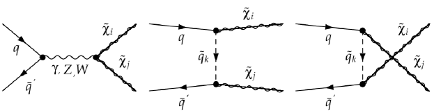
Figure 5.23: Tree-level Feynman diagrams for the production of gaugino pairs.

We consider the purely electroweak production of gaugino pairs

$$q(h_{a},p_{a})\,\bar{q}^{\prime}(h_{b},p_{b})\to\tilde{\chi}_{i}(p_{1})\,\tilde{\chi}_{j}(p_{2})$$ (5.33)

from quark-antiquark initial states, where flavour violation can occur via the quark-squark-gaugino vertices in the $t$- and $u$-channels (see Fig. 5.23). However, if it were not for different parton density weights, summation over complete squark multiplet exchanges would make these channels insensitive to the exchanged squark flavour. Furthermore there are no final state squarks that could be experimentally tagged. The cross section can be expressed generically as [97]

$$\frac{d\hat{\sigma}^{q\bar{q}^{\prime}}_{h_{a},h_{b}}}{dt} = \frac{\pi\alpha^{2}}{3s^{2}}(1-h_{a})(1+h_{b})\Big{[}\left|Q^{u}_{LL}\right|^{2}u_{\tilde{\chi}_{i}}u_{\tilde{\chi}_{j}}+\left|Q_{LL}^{t}\right|^{2}t_{\tilde{\chi}_{i}}t_{\tilde{\chi}_{j}}+2{\rm Re}[Q_{LL}^{u\ast}Q_{LL}^{t}]$$ (5.34)

$$\times m_{\tilde{\chi}_{i}}m_{\tilde{\chi}_{j}}s\Big{]}+\frac{\pi\alpha^{2}}{3s^{2}}(1+h_{a})(1-h_{b})\Big{[}\left|Q_{RR}^{u}\right|^{2}u_{\tilde{\chi}_{i}}u_{\tilde{\chi}_{j}}+\left|Q_{RR}^{t}\right|^{2}t_{\tilde{\chi}_{i}}t_{\tilde{\chi}_{j}}$$

$$+ 2{\rm Re}[Q_{RR}^{u\ast}Q_{RR}^{t}]m_{\tilde{\chi}_{i}}m_{\tilde{\chi}_{j}}s\Big{]}+\frac{\pi\alpha^{2}}{3s^{2}}(1+h_{a})(1+h_{b})\Big{[}\left|Q_{RL}^{u}\right|^{2}u_{\tilde{\chi}_{i}}u_{\tilde{\chi}_{j}}$$

$$+ \left|Q_{RL}^{t}\right|^{2}t_{\tilde{\chi}_{i}}t_{\tilde{\chi}_{j}}\!+\!{\rm Re}[Q_{RL}^{u\ast}Q_{RL}^{t}](ut\!-\!m^{2}_{\tilde{\chi}_{i}}m^{2}_{\tilde{\chi}_{j}})\Big{]}\!+\!\frac{\pi\alpha^{2}}{3s^{2}}(1\!-\!h_{a})(1\!-\!h_{b})$$

$$\times \Big{[}\left|Q_{LR}^{u}\right|^{2}u_{\tilde{\chi}_{i}}u_{\tilde{\chi}_{j}}\!+\!\left|Q_{LR}^{t}\right|^{2}t_{\tilde{\chi}_{i}}t_{\tilde{\chi}_{j}}\!+\!{\rm Re}[Q_{LR}^{u\ast}Q_{LR}^{t}](ut\!-\!m^{2}_{\tilde{\chi}_{i}}m^{2}_{\tilde{\chi}_{j}})\Big{]},\leavevmode\nobreak\ \leavevmode\nobreak\ \leavevmode\nobreak\ \leavevmode\nobreak\ \leavevmode\nobreak\$$

i.e. in terms of generalized charges. For $\tilde{\chi}_{i}^{-}\tilde{\chi}_{j}^{+}$-production, these charges are given by

$$Q_{LL}^{u-+} = \Bigg{(}\frac{e_{q}\delta_{ij}\delta_{qq^{\prime}}}{s}-\frac{L_{qq^{\prime}Z}O^{\prime R\ast}_{ij}}{2\,x_{W}\,(1-x_{W})\,s_{z}}+\sum_{k=1}^{6}\frac{L_{\tilde{d}_{k}q^{\prime}\tilde{\chi}_{i}^{\pm}}L^{\ast}_{\tilde{d}_{k}q\tilde{\chi}_{j}^{\pm}}}{2\,x_{W}\,u_{\tilde{d}_{k}}}\Bigg{)},\leavevmode\nobreak\$$

$$Q_{LL}^{t-+} = \Bigg{(}\frac{e_{q}\delta_{ij}\delta_{qq^{\prime}}}{s}-\frac{L_{qq^{\prime}Z}O^{\prime L\ast}_{ij}}{2\,x_{W}\,(1-x_{W})\,s_{z}}-\sum_{k=1}^{6}\frac{L^{\ast}_{\tilde{u}_{k}q^{\prime}\tilde{\chi}_{j}^{\pm}}L_{\tilde{u}_{k}q\tilde{\chi}_{i}^{\pm}}}{2\,x_{W}\,t_{\tilde{u}_{k}}}\Bigg{)},\leavevmode\nobreak\$$

$$Q_{RR}^{u-+} = \Bigg{(}\frac{e_{q}\delta_{ij}\delta_{qq^{\prime}}}{s}-\frac{R_{qq^{\prime}Z}O^{\prime L\ast}_{ij}}{2\,x_{W}\,(1-x_{W})\,s_{z}}+\sum_{k=1}^{6}\frac{R_{\tilde{d}_{k}q^{\prime}\tilde{\chi}_{i}^{\pm}}R^{\ast}_{\tilde{d}_{k}q\tilde{\chi}_{j}^{\pm}}}{2\,x_{W}\,u_{\tilde{d}_{k}}}\Bigg{)},\leavevmode\nobreak\$$

$$Q_{RR}^{t-+} = \Bigg{(}\frac{e_{q}\delta_{ij}\delta_{qq^{\prime}}}{s}-\frac{R_{qq^{\prime}Z}O^{\prime R\ast}_{ij}}{2\,x_{W}\,(1-x_{W})\,s_{z}}-\sum_{k=1}^{6}\frac{R^{\ast}_{\tilde{u}_{k}q^{\prime}\tilde{\chi}_{j}^{\pm}}R_{\tilde{u}_{k}q\tilde{\chi}_{i}^{\pm}}}{2\,x_{W}\,t_{\tilde{u}_{k}}}\Bigg{)},\leavevmode\nobreak\$$

$$Q_{LR}^{u-+} = \sum_{k=1}^{6}\frac{R_{\tilde{d}_{k}q^{\prime}\tilde{\chi}_{i}^{\pm}}L^{\ast}_{\tilde{d}_{k}q\tilde{\chi}_{j}^{\pm}}}{2\,x_{W}\,u_{\tilde{d}_{k}}},\leavevmode\nobreak\$$

$$Q_{LR}^{t-+} = \sum_{k=1}^{6}\frac{R^{\ast}_{\tilde{u}_{k}q^{\prime}\tilde{\chi}_{j}^{\pm}}L_{\tilde{u}_{k}q\tilde{\chi}_{i}^{\pm}}}{2\,x_{W}\,t_{\tilde{u}_{k}}},\leavevmode\nobreak\$$

$$Q_{RL}^{u-+} = \sum_{k=1}^{6}\frac{L_{\tilde{d}_{k}q^{\prime}\tilde{\chi}_{i}^{\pm}}R^{\ast}_{\tilde{d}_{k}q\tilde{\chi}_{j}^{\pm}}}{2\,x_{W}\,u_{\tilde{d}_{k}}},\leavevmode\nobreak\$$

$$Q_{RL}^{t-+} = \sum_{k=1}^{6}\frac{L^{\ast}_{\tilde{u}_{k}q^{\prime}\tilde{\chi}_{j}^{\pm}}R_{\tilde{u}_{k}q\tilde{\chi}_{i}^{\pm}}}{2\,x_{W}\,t_{\tilde{u}_{k}}}.$$ (5.35)

Note that there is no interference between $t$- and $u$-channel diagrams due to (electromagnetic) charge conservation. The cross section for chargino pair production in $e^{+}e^{-}$-collisions can be deduced by setting $e_{q}\to e_{l}=-1$, $L_{qq^{\prime}Z}\to L_{eeZ}=(2\,T^{3}_{l}-2\,e_{l}\,x_{W})$ and $R_{qq^{\prime}Z}\to R_{eeZ}=-2\,e_{l}\,x_{W}$. Neglecting all Yukawa couplings, we can then reproduce the calculations of Ref. [224].

The charges of the chargino-neutralino associated production are given by

$$Q_{LL}^{u+0} = \frac{1}{\sqrt{2\,(1-x_{W})}\,x_{W}}\left[\frac{O^{L\ast}_{ji}L^{\ast}_{qq^{\prime}W}}{\sqrt{2}\,s_{w}}+\sum_{k=1}^{6}\frac{L_{\tilde{u}_{k}q^{\prime}\tilde{\chi}_{i}^{\pm}}^{\ast}L_{\tilde{u}_{k}q\tilde{\chi}_{j}^{0}}^{\ast}}{u_{\tilde{u}_{k}}}\right],\leavevmode\nobreak\$$

$$Q_{LL}^{t+0} = \frac{1}{\sqrt{2\,(1-x_{W})}\,x_{W}}\left[\frac{O^{R\ast}_{ji}L^{\ast}_{qq^{\prime}W}}{\sqrt{2}\,s_{w}}-\sum_{k=1}^{6}\frac{L_{\tilde{d}_{k}q\tilde{\chi}_{i}^{\pm}}^{\ast}L_{\tilde{d}_{k}q^{\prime}\tilde{\chi}_{j}^{0}}}{t_{\tilde{d}_{k}}}\right],\leavevmode\nobreak\$$

$$Q_{RR}^{u+0} = \frac{1}{\sqrt{2\,(1-x_{W})}\,x_{W}}\sum_{k=1}^{6}\frac{R_{\tilde{u}_{k}q^{\prime}\tilde{\chi}_{i}^{\pm}}^{\ast}R_{\tilde{u}_{k}q\tilde{\chi}_{j}^{0}}^{\ast}}{u_{\tilde{u}_{k}}},\leavevmode\nobreak\$$

$$Q_{RR}^{t+0} = \frac{-1}{\sqrt{2\,(1-x_{W})}\,x_{W}}\sum_{k=1}^{6}\frac{R_{\tilde{d}_{k}q\tilde{\chi}_{i}^{\pm}}^{\ast}R_{\tilde{d}_{k}q^{\prime}\tilde{\chi}_{j}^{0}}}{t_{\tilde{d}_{k}}},\leavevmode\nobreak\$$

$$Q_{LR}^{u+0} = \frac{1}{\sqrt{2\,(1-x_{W})}\,x_{W}}\sum_{k=1}^{6}\frac{R_{\tilde{u}_{k}q^{\prime}\tilde{\chi}_{i}^{\pm}}^{\ast}L_{\tilde{u}_{k}q\tilde{\chi}_{j}^{0}}^{\ast}}{u_{\tilde{u}_{k}}},\leavevmode\nobreak\$$

$$Q_{LR}^{t+0} = \frac{1}{\sqrt{2\,(1-x_{W})}\,x_{W}}\sum_{k=1}^{6}\frac{L_{\tilde{d}_{k}q\tilde{\chi}_{i}^{\pm}}^{\ast}R_{\tilde{d}_{k}q^{\prime}\tilde{\chi}_{j}^{0}}}{t_{\tilde{d}_{k}}},\leavevmode\nobreak\$$

$$Q_{RL}^{u+0} = \frac{1}{\sqrt{2\,(1-x_{W})}\,x_{W}}\sum_{k=1}^{6}\frac{L_{\tilde{u}_{k}q^{\prime}\tilde{\chi}_{i}^{\pm}}^{\ast}R_{\tilde{u}_{k}q\tilde{\chi}_{j}^{0}}^{\ast}}{u_{\tilde{u}_{k}}},\leavevmode\nobreak\$$

$$Q_{RL}^{t+0} = \frac{1}{\sqrt{2\,(1-x_{W})}\,x_{W}}\sum_{k=1}^{6}\frac{R_{\tilde{d}_{k}q\tilde{\chi}_{i}^{\pm}}^{\ast}L_{\tilde{d}_{k}q^{\prime}\tilde{\chi}_{j}^{0}}}{t_{\tilde{d}_{k}}}.$$ (5.36)

The charge-conjugate process is again obtained by making the replacement $h_{a,b}\to-h_{a,b}$ in Eq. (5.34). In the case of non-mixing squarks with neglected Yukawa couplings, we agree with the results of Ref. [40], provided we correct a sign in their Eq. (2) as described in Ref. [225].

Finally, the charges for the neutralino pair production are given by

$$Q_{LL}^{u00} = \frac{1}{x_{W}\,(1-x_{W})\,\sqrt{1+\delta_{ij}}}\left[\frac{L_{qq^{\prime}Z}O^{\prime\prime L}_{ij}}{2s_{z}}+\sum_{k=1}^{6}\frac{L_{\tilde{Q}_{k}q^{\prime}\tilde{\chi}_{i}^{0}}L_{\tilde{Q}_{k}q\tilde{\chi}_{j}^{0}}^{\ast}}{u_{\tilde{Q}_{k}}}\right],\leavevmode\nobreak\$$

$$Q_{LL}^{t00} = \frac{1}{x_{W}\,(1-x_{W})\,\sqrt{1+\delta_{ij}}}\left[\frac{L_{qq^{\prime}Z}O^{\prime\prime R}_{ij}}{2s_{z}}-\sum_{k=1}^{6}\frac{L_{\tilde{Q}_{k}q\tilde{\chi}_{i}^{0}}^{\ast}L_{\tilde{Q}_{k}q^{\prime}\tilde{\chi}_{j}^{0}}}{t_{\tilde{Q}_{k}}}\right],\leavevmode\nobreak\$$

$$Q_{RR}^{u00} = \frac{1}{x_{W}\,(1-x_{W})\,\sqrt{1+\delta_{ij}}}\left[\frac{R_{qq^{\prime}Z}O^{\prime\prime R}_{ij}}{2s_{z}}+\sum_{k=1}^{6}\frac{R_{\tilde{Q}_{k}q^{\prime}\tilde{\chi}_{i}^{0}}R_{\tilde{Q}_{k}q\tilde{\chi}_{j}^{0}}^{\ast}}{u_{\tilde{Q}_{k}}}\right],\leavevmode\nobreak\$$

$$Q_{RR}^{t00} = \frac{1}{x_{W}\,(1-x_{W})\,\sqrt{1+\delta_{ij}}}\left[\frac{R_{qq^{\prime}Z}O^{\prime\prime L}_{ij}}{2s_{z}}-\sum_{k=1}^{6}\frac{R_{\tilde{Q}_{k}q\tilde{\chi}_{i}^{0}}^{\ast}R_{\tilde{Q}_{k}q^{\prime}\tilde{\chi}_{j}^{0}}}{t_{\tilde{Q}_{k}}}\right],\leavevmode\nobreak\$$

$$Q_{LR}^{u00} = \frac{1}{x_{W}\,(1-x_{W})\,\sqrt{1+\delta_{ij}}}\sum_{k=1}^{6}\frac{R_{\tilde{Q}_{k}q^{\prime}\tilde{\chi}_{i}^{0}}L_{\tilde{Q}_{k}q\tilde{\chi}_{j}^{0}}^{\ast}}{u_{\tilde{Q}_{k}}},\leavevmode\nobreak\$$

$$Q_{LR}^{t00} = \frac{1}{x_{W}\,(1-x_{W})\,\sqrt{1+\delta_{ij}}}\sum_{k=1}^{6}\frac{L_{\tilde{Q}_{k}q\tilde{\chi}_{i}^{0}}^{\ast}R_{\tilde{Q}_{k}q^{\prime}\tilde{\chi}_{j}^{0}}}{t_{\tilde{Q}_{k}}},\leavevmode\nobreak\$$

$$Q_{RL}^{u00} = \frac{1}{x_{W}\,(1-x_{W})\,\sqrt{1+\delta_{ij}}}\sum_{k=1}^{6}\frac{L_{\tilde{Q}_{k}q^{\prime}\tilde{\chi}_{i}^{0}}R_{\tilde{Q}_{k}q\tilde{\chi}_{j}^{0}}^{\ast}}{u_{\tilde{Q}_{k}}},\leavevmode\nobreak\$$

$$Q_{RL}^{t00} = \frac{1}{x_{W}\,(1-x_{W})\,\sqrt{1+\delta_{ij}}}\sum_{k=1}^{6}\frac{R_{\tilde{Q}_{k}q\tilde{\chi}_{i}^{0}}^{\ast}L_{\tilde{Q}_{k}q^{\prime}\tilde{\chi}_{j}^{0}}}{t_{\tilde{Q}_{k}}},$$ (5.37)

which agrees with the results of Ref. [226] in the case of non-mixing squarks.

5.4.2 Numerical results

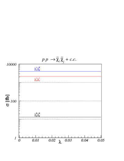
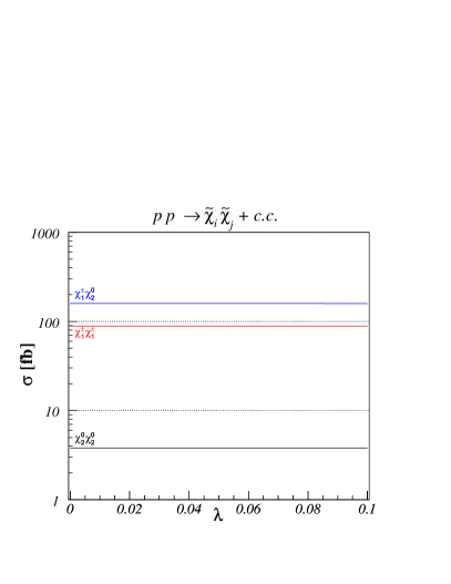
Figure 5.24: Cross sections for gaugino pair production at the LHC in our benchmark scenario A (left) and B (right).

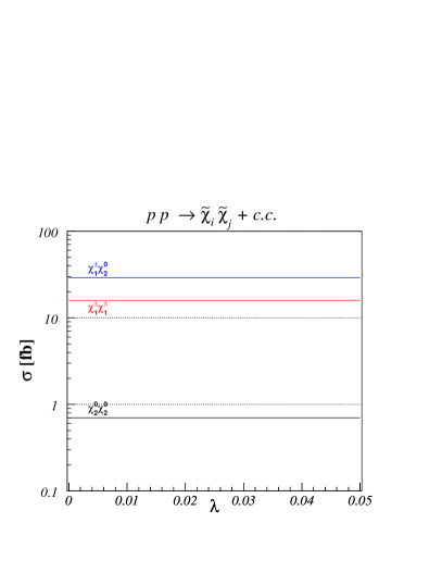
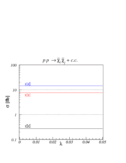
Figure 5.25: Same as Fig. 5.24 for our benchmark scenario C (left) and D (right).

As in the previous sections, the SUSY masses and mixings are computed with the help of SPheno and FeynHiggs, and the LO set of the CTEQ6 parton density are used. The numerical cross sections for gaugino pair production are shown in Figs. 5.24 and 5.25 for our benchmark scenario A, B, C, and D. Their cross sections are rather large, but practically insensitive to the flavour violation parameter $\lambda$, since they are summed over exchanged squark flavours.

5.5 Impact of flavour violation on squark and gaugino production

In the previous sections, we have performed an extensive analysis of squark and gaugino hadroproduction and decays in non-minimal flavour violating supersymmetry. Within the super-CKM basis, we have taken into account the possible misalignment of quark and squark rotations and computed all squared helicity amplitudes for the production and the decay widths of squarks and gauginos in compact analytic form, verifying that our results agree with the literature in the case of non-mixing squarks whenever possible. In order to obtain numerical predictions for hadron colliders, we have implemented all our results in a flexible computer program, allowing us to discuss in detail the dependence of the cross section on flavour violation. An illustrative summary of flavour violating hadroproduction cross section contributions for third-generation squarks and/or gauginos is presented in Tab. 5.1, together with the competing flavour-diagonal contributions, which are the only contributions in cMFV SUSY.

Table 5.1: Dominant $s$-, $t$-, and $u$-channel contributions to the flavour violating hadroproduction of third-generation squarks and/or gauginos and the competing dominant flavour-diagonal contributions.

Exchange	$s$	$t$	$u$
Final State
$\tilde{t}\tilde{b}^{*}$	$W$	NMFV-$\tilde{g}$	-
$\tilde{b}\tilde{s}^{*}$	NMFV-$Z$	NMFV-$\tilde{g}$	-
$\tilde{t}\tilde{c}^{*}$	NMFV-$Z$	NMFV-$\tilde{g}$	-
$\tilde{t}\tilde{b}$	-	-	NMFV-$\tilde{g}$
$\tilde{b}\tilde{b}$	-	$\tilde{g}$	$\tilde{g}$
$\tilde{t}\tilde{t}$	-	NMFV-$\tilde{g}$	NMFV-$\tilde{g}$
$\tilde{\chi}^{0}\tilde{b}$	$b$	$\tilde{b}$	-
$\tilde{\chi}^{\pm}\tilde{b}$	NMFV-$c$	NMFV-$\tilde{b}$	-
$\tilde{\chi}^{0}\tilde{t}$	NMFV-$c$	NMFV-$\tilde{t}$	-
$\tilde{\chi}^{\pm}\tilde{t}$	$b$	$\tilde{t}$	-
$\tilde{\chi}\tilde{\chi}$	$\gamma,Z,W$	$\tilde{q}$	$\tilde{q}$

5.6 NMFV decays of squarks, gluino and gauginos

5.6.1 Squark decays

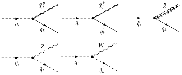
Figure 5.26: Tree-level Feynman diagrams for squark decays into gauginos and quarks (top) and into electroweak gauge bosons and lighter squarks (bottom).

We turn now from SUSY particle production to decay processes and show in Fig. 5.26 the possible decays of squarks into gauginos and quarks (top) as well as into electroweak gauge bosons and lighter squarks (bottom). Both processes can in general induce flavour violation. The decay widths of the former are given by

$$\Gamma_{\tilde{q}_{i}\to\tilde{\chi}^{0}_{j}q_{k}} = \frac{\alpha}{2\,m^{3}_{\tilde{q}_{i}}\,x_{W}\,(1-x_{W})}\Bigg{(}\bigg{(}m^{2}_{\tilde{q}_{i}}-m^{2}_{\tilde{\chi}^{0}_{j}}-m^{2}_{q_{k}}\bigg{)}\bigg{(}\left|L_{\tilde{q}_{i}q_{k}\tilde{\chi}_{j}^{0}}\right|^{2}+\left|R_{\tilde{q}_{i}q_{k}\tilde{\chi}_{j}^{0}}\right|^{2}\bigg{)}$$ (5.38)

$$- 4\,m_{\tilde{\chi}^{0}_{j}}\,m_{q_{k}}\,{\rm Re}\left[L_{\tilde{q}_{i}q_{k}\tilde{\chi}_{j}^{0}}R^{\ast}_{\tilde{q}_{i}q_{k}\tilde{\chi}_{j}^{0}}\right]\Bigg{)}\,\lambda^{1/2}(m^{2}_{\tilde{q}_{i}},m^{2}_{\tilde{\chi}^{0}_{j}},m^{2}_{q_{k}}),\leavevmode\nobreak\$$

$$\Gamma_{\tilde{q}_{i}\to\tilde{\chi}^{\pm}_{j}q^{\prime}_{k}} = \frac{\alpha}{4\,m^{3}_{\tilde{q}_{i}}\,x_{W}}\Bigg{(}\bigg{(}m^{2}_{\tilde{q}_{i}}-m^{2}_{\tilde{\chi}^{\pm}_{j}}-m^{2}_{q^{\prime}_{k}}\bigg{)}\bigg{(}\left|L_{\tilde{q}_{i}q^{\prime}_{k}\tilde{\chi}_{j}^{\pm}}\right|^{2}+\left|R_{\tilde{q}_{i}q^{\prime}_{k}\tilde{\chi}_{j}^{\pm}}\right|^{2}\bigg{)}$$ (5.39)

$$- 4\,m_{\tilde{\chi}^{\pm}_{j}}\,m_{q^{\prime}_{k}}\,{\rm Re}\left[L_{\tilde{q}_{i}q^{\prime}_{k}\tilde{\chi}_{j}^{\pm}}R^{\ast}_{\tilde{q}_{i}q^{\prime}_{k}\tilde{\chi}_{j}^{\pm}}\right]\Bigg{)}\,\lambda^{1/2}(m^{2}_{\tilde{q}_{i}},m^{2}_{\tilde{\chi}^{\pm}_{j}},m^{2}_{q^{\prime}_{k}}),\leavevmode\nobreak\$$

$$\Gamma_{\tilde{q}_{i}\to\tilde{g}q_{k}} = \frac{2\,\alpha_{s}}{3\,m^{3}_{\tilde{q}_{i}}\,x_{W}}\Bigg{(}\bigg{(}m^{2}_{\tilde{q}_{i}}-m^{2}_{\tilde{g}}-m^{2}_{q_{k}}\bigg{)}\bigg{(}\left|L_{\tilde{q}_{i}q_{k}\tilde{g}}\right|^{2}+\left|R_{\tilde{q}_{i}q_{k}\tilde{g}}\right|^{2}\bigg{)}$$ (5.40)

$$- 4\,m_{\tilde{g}}\,m_{q_{k}}\,{\rm Re}\left[L_{\tilde{q}_{i}q_{k}\tilde{g}}R^{\ast}_{\tilde{q}_{i}q_{k}\tilde{g}}\right]\Bigg{)}\,\lambda^{1/2}(m^{2}_{\tilde{q}_{i}},m^{2}_{\tilde{g}},m^{2}_{q_{k}}),$$

while those of the latter are given by

$$\Gamma_{\tilde{q}_{i}\to Z\tilde{q}_{k}} = \frac{\alpha}{16\,m^{3}_{\tilde{q}_{i}}\,m^{2}_{Z}x_{W}(1-x_{W})}\left|L_{\tilde{q}_{i}\tilde{q}_{k}Z}\!+\!R_{\tilde{q}_{i}\tilde{q}_{k}Z}\right|^{2}\,\lambda^{3/2}(m^{2}_{\tilde{q}_{i}},m^{2}_{Z},m^{2}_{\tilde{q}_{k}}),\leavevmode\nobreak\ \leavevmode\nobreak\ \leavevmode\nobreak\ \leavevmode\nobreak\ \leavevmode\nobreak\ \leavevmode\nobreak\$$ (5.41)

$$\Gamma_{\tilde{q}_{i}\to W^{\pm}\tilde{q}^{\prime}_{k}} = \frac{\alpha}{16\,m^{3}_{\tilde{q}_{i}}\,m^{2}_{W}\,x_{W}\,(1-x_{W})}\left|L_{\tilde{q}_{i}\tilde{q}^{\prime}_{k}W}\right|^{2}\,\lambda^{3/2}(m^{2}_{\tilde{q}_{i}},m^{2}_{W},m^{2}_{\tilde{q}^{\prime}_{k}}).$$ (5.42)

The usual Källen function is

$$\lambda(x,y,z)=x^{2}+y^{2}+z^{2}-2(x\,y+y\,z+z\,x).$$ (5.43)

In MFV, our results agree with those of Ref. [227].

5.6.2 Gluino decays

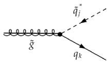
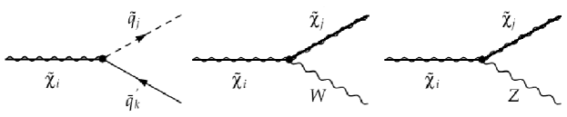
Figure 5.27: Tree-level Feynman diagram for gluino decays into squarks and quarks.

Figure 5.28: Tree-level Feynman diagrams for gaugino decays into squarks and quarks (left) and into lighter gauginos and electroweak gauge bosons (centre and right).

Heavy gluinos can decay strongly into squarks and quarks as shown in Fig. 5.28. The corresponding decay width

$$\Gamma_{\tilde{g}\to\tilde{q}^{\ast}_{j}q_{k}} = \frac{\alpha_{s}}{8\,m^{3}_{\tilde{g}}}\Bigg{(}\bigg{(}m^{2}_{\tilde{g}}-m^{2}_{\tilde{q}_{j}}+m^{2}_{q_{k}}\bigg{)}\bigg{(}\left|L_{\tilde{q}_{j}q_{k}\tilde{g}}\right|^{2}+\left|R_{\tilde{q}_{j}q_{k}\tilde{g}}\right|^{2}\bigg{)}$$ (5.44)

$$+ 4\,m_{\tilde{g}}\,m_{q_{k}}\,{\rm Re}\left[L_{\tilde{q}_{j}q_{k}\tilde{g}}R^{\ast}_{\tilde{q}_{j}q_{k}\tilde{g}}\right]\Bigg{)}\,\lambda^{1/2}(m^{2}_{\tilde{g}},m^{2}_{\tilde{q}_{j}},m^{2}_{q_{k}})$$

can in general also induce flavour violation. In MFV, our result agrees again with the one of Ref. [227].

5.6.3 Gaugino decays

Heavier gauginos can decay into squarks and quarks as shown in Fig. 5.28 (left) or into lighter gauginos and electroweak gauge bosons (Fig. 5.28 centre and right). The analytical decay widths are

$$\Gamma_{\tilde{\chi}_{i}^{\pm}\to\tilde{q}_{j}\bar{q}^{\prime}_{k}} = \frac{3\,\alpha}{8\,m^{3}_{\tilde{\chi}_{i}^{\pm}}\,x_{W}}\Bigg{(}\bigg{(}m^{2}_{\tilde{\chi}_{i}^{\pm}}-m^{2}_{\tilde{q}_{j}}+m^{2}_{q^{\prime}_{k}}\bigg{)}\bigg{(}\left|L_{\tilde{q}_{j}q^{\prime}_{k}\tilde{\chi}_{i}^{\pm}}\right|^{2}+\left|R_{\tilde{q}_{j}q^{\prime}_{k}\tilde{\chi}_{i}^{\pm}}\right|^{2}\bigg{)}$$ (5.45)

$$+ 4\,m_{\tilde{\chi}_{i}^{\pm}}\,m_{q^{\prime}_{k}}\,{\rm Re}\left[L_{\tilde{q}_{j}q^{\prime}_{k}\tilde{\chi}_{i}^{\pm}}R^{\ast}_{\tilde{q}_{j}q^{\prime}_{k}\tilde{\chi}_{i}^{\pm}}\right]\Bigg{)}\,\lambda^{1/2}(m^{2}_{\tilde{\chi}_{i}^{\pm}},m^{2}_{\tilde{q}_{j}},m^{2}_{q^{\prime}_{k}})$$

and

$$\Gamma_{\tilde{\chi}_{i}^{\pm}\to\tilde{\chi}_{j}^{0}W^{\pm}} = \frac{\alpha}{8\,m^{3}_{\tilde{\chi}_{i}^{\pm}}m_{W}^{2}x_{W}}\Bigg{(}\bigg{(}m^{4}_{\tilde{\chi}_{i}^{\pm}}+m^{4}_{\tilde{\chi}_{j}^{0}}-2\,m^{4}_{W}+m^{2}_{\tilde{\chi}_{i}^{\pm}}\,m^{2}_{W}+m^{2}_{\tilde{\chi}_{j}^{0}}\,m^{2}_{W}$$ (5.46)

$$- 2\,m^{2}_{\tilde{\chi}_{i}^{\pm}}\,m^{2}_{\tilde{\chi}_{j}^{0}}\bigg{)}\,\bigg{(}\left|O^{L}_{ij}\right|^{2}+\left|O^{R}_{ij}\right|^{2}\bigg{)}-12\,m_{\tilde{\chi}_{i}^{\pm}}\,m_{W}^{2}\,m_{\tilde{\chi}_{j}^{0}}\,{\rm Re}\left[O^{L}_{ij}O^{R\ast}_{ij}\right]\Bigg{)}$$

$$\times \lambda^{1/2}(m^{2}_{\tilde{\chi}_{i}^{\pm}},m^{2}_{\tilde{\chi}_{j}^{0}},m^{2}_{W}),\leavevmode\nobreak\$$

$$\Gamma_{\tilde{\chi}_{i}^{\pm}\to\tilde{\chi}_{j}^{\pm}Z} = \frac{\alpha}{8\,m^{3}_{\tilde{\chi}_{i}^{\pm}}m_{Z}^{2}x_{W}(1\!-\!x_{W})}\Bigg{(}\bigg{(}m^{4}_{\tilde{\chi}_{i}^{\pm}}\!+\!m^{4}_{\tilde{\chi}_{j}^{\pm}}\!-\!2\,m^{4}_{Z}\!+\!m^{2}_{\tilde{\chi}_{i}^{\pm}}\,m^{2}_{Z}\!+\!m^{2}_{\tilde{\chi}_{j}^{\pm}}\,m^{2}_{Z}$$ (5.47)

$$- 2\,m^{2}_{\tilde{\chi}_{i}^{\pm}}\,m^{2}_{\tilde{\chi}_{j}^{\pm}}\bigg{)}\,\bigg{(}\left|O^{\prime L}_{ij}\right|^{2}+\left|O^{\prime R}_{ij}\right|^{2}\bigg{)}-12\,m_{\tilde{\chi}_{i}^{\pm}}\,m_{Z}^{2}\,m_{\tilde{\chi}_{j}^{\pm}}\,{\rm Re}\left[O^{\prime L}_{ij}O^{\prime R\ast}_{ij}\right]\Bigg{)}$$

$$\times \lambda^{1/2}(m^{2}_{\tilde{\chi}_{i}^{\pm}},m^{2}_{\tilde{\chi}_{j}^{\pm}},m^{2}_{Z})$$

for charginos and

$$\Gamma_{\tilde{\chi}_{i}^{0}\to\tilde{q}_{j}\bar{q}_{k}} = \frac{3\,\alpha}{4\,m^{3}_{\tilde{\chi}_{i}^{0}}\,x_{W}\,(1-x_{W})}\Bigg{(}\bigg{(}m^{2}_{\tilde{\chi}_{i}^{0}}-m^{2}_{\tilde{q}_{j}}+m^{2}_{q_{k}}\bigg{)}\bigg{(}\left|L_{\tilde{q}_{j}q_{k}\tilde{\chi}_{i}^{0}}\right|^{2}+\left|R_{\tilde{q}_{j}q_{k}\tilde{\chi}_{i}^{0}}\right|^{2}\bigg{)}$$ (5.48)

$$+ 4\,m_{\tilde{\chi}_{i}^{0}}\,m_{q_{k}}\,{\rm Re}\left[L_{\tilde{q}_{j}q_{k}\tilde{\chi}_{i}^{0}}R^{\ast}_{\tilde{q}_{j}q_{k}\tilde{\chi}_{i}^{0}}\right]\Bigg{)}\,\lambda^{1/2}(m^{2}_{\tilde{\chi}_{i}^{0}},m^{2}_{\tilde{q}_{j}},m^{2}_{q_{k}})$$

and

$$\Gamma_{\tilde{\chi}_{i}^{0}\to\tilde{\chi}_{j}^{\pm}W^{\mp}} = \frac{\alpha}{8\,m^{3}_{\tilde{\chi}_{i}^{0}}\,m_{W}^{2}\,x_{W}}\Bigg{(}\bigg{(}m^{4}_{\tilde{\chi}_{i}^{0}}+m^{4}_{\tilde{\chi}_{j}^{\pm}}-2\,m^{4}_{W}+m^{2}_{\tilde{\chi}_{i}^{0}}\,m^{2}_{W}+m^{2}_{\tilde{\chi}_{j}^{\pm}}\,m^{2}_{W}$$ (5.49)

$$- 2\,m^{2}_{\tilde{\chi}_{i}^{0}}\,m^{2}_{\tilde{\chi}_{j}^{\pm}}\bigg{)}\,\bigg{(}\left|O^{L}_{ij}\right|^{2}+\left|O^{R}_{ij}\right|^{2}\bigg{)}-12\,m_{\tilde{\chi}_{i}^{0}}\,m_{W}^{2}\,m_{\tilde{\chi}_{j}^{\pm}}\,{\rm Re}\left[O^{L}_{ij}O^{R\ast}_{ij}\right]\Bigg{)}$$

$$\times \lambda^{1/2}(m^{2}_{\tilde{\chi}_{i}^{0}},m^{2}_{\tilde{\chi}_{j}^{\pm}},m^{2}_{W}),\leavevmode\nobreak\$$

$$\Gamma_{\tilde{\chi}_{i}^{0}\to\tilde{\chi}_{j}^{0}Z} = \frac{\alpha}{8\,m^{3}_{\tilde{\chi}_{i}^{0}}\,m_{Z}^{2}\,x_{W}\,(1-x_{W})}\Bigg{(}\bigg{(}m^{4}_{\tilde{\chi}_{i}^{0}}+m^{4}_{\tilde{\chi}_{j}^{0}}-2\,m^{4}_{Z}+m^{2}_{\tilde{\chi}_{i}^{0}}\,m^{2}_{Z}+m^{2}_{\tilde{\chi}_{j}^{0}}\,m^{2}_{Z}$$ (5.50)

$$- 2\,m^{2}_{\tilde{\chi}_{i}^{0}}\,m^{2}_{\tilde{\chi}_{j}^{0}}\bigg{)}\,\bigg{(}\left|O^{\prime L}_{ij}\right|^{2}+\left|O^{\prime R}_{ij}\right|^{2}\bigg{)}-12\,m_{\tilde{\chi}_{i}^{0}}\,m_{Z}^{2}\,m_{\tilde{\chi}_{j}^{0}}\,{\rm Re}\left[O^{\prime\prime L}_{ij}O^{\prime\prime R\ast}_{ij}\right]\Bigg{)}$$

$$\times \lambda^{1/2}(m^{2}_{\tilde{\chi}_{i}^{0}},m^{2}_{\tilde{\chi}_{j}^{0}},m^{2}_{Z})$$

for neutralinos, respectively. Chargino decays into a slepton and a neutrino (lepton and sneutrino) can be deduced from the previous equations by taking the proper limits, i.e. by removing colour factors and down-type masses in the coupling definitions. Our results agree then with those of Ref. [228] in the limit of non-mixing sneutrinos. Note that the same simplifications also permit a verification of our results for squark decays into a gaugino and a quark in Eqs. (5.38) and (5.39) when compared to their leptonic counterparts in Ref. [228].

  

Chapter 6 Conclusion and outlook

The Standard Model of particle physics provides a successful description of presently known phenomena, except for neutrino physics. However, despite of its success, a set of conceptual problems do not have a solution within the framework of the SM, such as the origin of mass, gauge coupling unification, or the hierarchy problem. Several attempts have been made to solve these problems, leading to various theories beyond the SM, even if there is still no experimental evidence of their existence. Each of these theories predicts new particles, with masses lying in the TeV-range, i.e. the discovery reach of present and future hadron colliders, the Tevatron and the LHC, which will then be able to put constraints on these models, or conclude about their (non-)existence.

In this thesis, we have considered the production of sleptons, squarks and gauginos of the Minimal Supersymmetric Standard Model. Cross sections for SUSY particles production at hadron colliders have been extensively studied in the past at leading order and also at next-to-leading order of perturbative QCD, since they are expected to receive important contributions from radiative corrections. These corrections include large logarithms, which have to be resummed in order to get reliable perturbative results. We have thus performed a first and extensive study of the resummation effects for SUSY particle pair production at hadron colliders, focusing on Drell-Yan like slepton-pair and slepton-sneutrino associated production in minimal supergravity and gauge-mediated SUSY-breaking scenarios. We have presented accurate transverse-momentum and invariant-mass distributions, as well as total cross sections, resumming soft-gluon emission contributions to all orders in the strong coupling.

Monte Carlo event generators are also commonly used, especially by experimentalists, to calculate observables depending on the soft-gluon emission from the initial state partons in hadronic collisions. This allows to compare experimental data to theoretical predictions and to simulate experimental signatures, when there are no experimental data yet. These programs usually implement the hard scattering process at the leading order, matching it with parton showering, the latter parameterizing the initial- and final-state radiation. Let us note that recently, event generators using next-to-leading order calculations have also been developed. It is expected that both Monte Carlo parton showering and resummation calculations should accurately describe the effects of soft-gluon emission from the incoming partons. A comparison between the predictions given by the two approaches would certainly be useful in testing their reliability. Finally, other SUSY particle production processes, such as gaugino- or squark pair hadroproduction should also be considered.

The quest for supersymmetric particles at hadron colliders will nevertheless rely on our ability of predicting both the SUSY signal and the SM processes being the backgrounds for these searches. In this work, we have focused on presenting accurate predictions for a slepton-pair signal, i.e. two highly energetic lepton and a large amount of missing energy. We have not considered the background consisting mainly in lepton pairs coming from $WW$ and $t\bar{t}$ decays. A detailed phenomenological study, including all background contributions, remains to be performed, in order to propose proper experimental cuts to enhance the signal over the background ratio. Furthermore, the sensitivity of these cuts to a complete experimental environment should also be investigated.

In non-minimal supersymmetric models, novel effects of flavour violation may occur. In this case, the flavour structure in the squark sector cannot be directly deduced from the trilinear Yukawa couplings of the fermion and Higgs supermultiplets. We have performed a precise numerical analysis of the experimentally allowed parameter space, considering minimal supergravity scenarios with non-minimal flavour violation, looking for regions allowed by low-energy, electroweak precision, and cosmological data. Leading order cross sections for the production of squarks and gauginos at hadron colliders have been implemented in a flexible computer program, allowing us to study in detail the dependence of these cross sections on flavour violation.

A full experimental study including heavy-flavour tagging efficiencies, detector resolutions, and background processes would, of course, be very interesting in order to establish the experimental significance of NMFV. While the implementation of our analytical results in a general-purpose Monte Carlo generator should now be straight-forward, such a detailed experimental study is beyond the scope of this work. Other possible extensions of our work include the investigation of other SUSY-breaking mechanisms or the computation of the radiative corrections for all of these processes within the NMFV framework.

References

- [1] S. L. Glashow, Nucl. Phys. 22 (1961) 579.
- [2] S. Weinberg, Phys. Rev. Lett. 19 (1967) 1264.
- [3] S. L. Glashow, J. Iliopoulos and L. Maiani, Phys. Rev. D 2 (1970) 1285.
- [4] S. Weinberg, Phys. Rev. D 5 (1972) 1962.
- [5] D. J. Gross and F. Wilczek, Phys. Rev. D 8 (1973) 3633.
- [6] D. J. Gross and F. Wilczek, Phys. Rev. D 9 (1974) 980.
- [7] H. D. Politzer, Phys. Rept. 14 (1974) 129.
- [8] H. Georgi and S. L. Glashow, Phys. Rev. Lett. 32 (1974) 438.
- [9] H. Georgi, H. R. Quinn and S. Weinberg, Phys. Rev. Lett. 33 (1974) 451.
- [10] H. Fritzsch and P. Minkowski, Annals Phys. 93 (1975) 193.
- [11] N. Arkani-Hamed, S. Dimopoulos and G. R. Dvali, Phys. Lett. B 429 (1998) 263.
- [12] L. Randall and R. Sundrum, Phys. Rev. Lett. 83 (1999) 3370.
- [13] N. Arkani-Hamed, A. G. Cohen and H. Georgi, Phys. Lett. B 513 (2001) 232.
- [14] M. Schmaltz and D. Tucker-Smith, Ann. Rev. Nucl. Part. Sci. 55 (2005) 229.
- [15] Z. Chacko, H. S. Goh and R. Harnik, Phys. Rev. Lett. 96 (2006) 231802.
- [16] J. Wess and B. Zumino, Nucl. Phys. B 70 (1974) 39.
- [17] P. Fayet and S. Ferrara, Phys. Rept. 32 (1977) 249.
- [18] P. Fayet, Phys. Lett. B 69 (1977) 489.
- [19] G. R. Farrar and P. Fayet, Phys. Lett. B 76 (1978) 575.
- [20] P. Fayet, Phys. Lett. B 84 (1979) 416.
- [21] H. P. Nilles, Phys. Rept. 110 (1984) 1.
- [22] H. E. Haber and G. L. Kane, Phys. Rept. 117 (1985) 75.
- [23] E. Witten, Nucl. Phys. B 188 (1981) 513.
- [24] R. K. Kaul, Phys. Lett. B 109 (1982) 19.
- [25] L. E. Ibanez and G. G. Ross, Phys. Lett. B 105 (1981) 439.
- [26] S. Dimopoulos, S. Raby and F. Wilczek, Phys. Rev. D 24 (1981) 1681.
- [27] U. Amaldi, W. de Boer and H. Fürstenau, Phys. Lett. B 260 (1991) 447.
- [28] M. Carena, S. Pokorski and C. E. M. Wagner, Nucl. Phys. B 406 (1993) 59.
- [29] H. Goldberg, Phys. Rev. Lett. 50 (1983) 1419.
- [30] J. R. Ellis, J. S. Hagelin, D. V. Nanopoulos, K. A. Olive and M. Srednicki, Nucl. Phys. B 238 (1984) 453.
- [31] S. Dawson, E. Eichten and C. Quigg, Phys. Rev. D 31 (1985) 1581.
- [32] F. del Aguila and L. Ametller, Phys. Lett. B 261 (1991) 326.
- [33] H. Baer, C. H. Chen, F. Paige and X. Tata, Phys. Rev. D 49 (1994) 3283.
- [34] W. Beenakker, R. Höpker, M. Spira and P. M. Zerwas, Nucl. Phys. B 492 (1997) 51.
- [35] W. Beenakker, M. Krämer, T. Plehn, M. Spira and P. M. Zerwas, Nucl. Phys. B 515 (1998) 3.
- [36] E. L. Berger, M. Klasen and T. Tait, Phys. Rev. D 59 (1999) 074024.
- [37] E. L. Berger, M. Klasen and T. Tait, Phys. Lett. B 459 (1999) 165.
- [38] E. L. Berger, M. Klasen and T. Tait, Phys. Rev. D 62 (2000) 095014 [Erratum-ibid. D 67 (2003) 099901].
- [39] H. Baer, B. W. Harris and M. H. Reno, Phys. Rev. D 57 (1998) 5871.
- [40] W. Beenakker, M. Klasen, M. Krämer, T. Plehn, M. Spira and P. M. Zerwas, Phys. Rev. Lett. 83 (1999) 3780.
- [41] N. S. Craigie, K. Hidaka and P. Ratcliffe, Phys. Lett. B 129 (1983) 310.
- [42] N. S. Craigie, K. Hidaka, M. Jacob and F. M. Renard, Phys. Rept. 99 (1983) 69.
- [43] T. Gehrmann, D. Maitre and D. Wyler, Nucl. Phys. B 703 (2004) 147.
- [44] P. Chiappetta, J. Soffer and P. Taxil, Phys. Lett. B 162 (1985) 192.
- [45] B. C. Allanach et al., Eur. Phys. J. C 25 (2002) 113.
- [46] J. A. Aguilar-Saavedra et al., Eur. Phys. J. C 46 (2006) 43.
- [47] G. Bozzi, B. Fuks and M. Klasen, Phys. Lett. B 609 (2005) 339.
- [48] E. Lytken, Czech. J. Phys. 54 (2004) A169.
- [49] Yu. M. Andreev, S. I. Bityukov and N. V. Krasnikov, Phys. Atom. Nucl. 68 (2005) 340.
- [50] C. G. Lester and D. J. Summers, Phys. Lett. B 463 (1999) 99.
- [51] A. J. Barr, JHEP 0602 (2006) 042.
- [52] Y. L. Dokshitzer, D. Diakonov and S. I. Troian, Phys. Rept. 58 (1980) 269.
- [53] G. Parisi and R. Petronzio, Nucl. Phys. B 154, (1979) 427.
- [54] G. Curci, M. Greco and Y. Srivastava, Nucl. Phys. B 159 (1979) 451.
- [55] J. Kodaira and L. Trentadue, Phys. Lett. B 112 (1982) 66.
- [56] J. C. Collins and D. E. Soper, Nucl. Phys. B 193 (1981) 381 [Erratum-ibid. B 213 (1983) 545].
- [57] J. C. Collins and D. E. Soper, Nucl. Phys. B 197 (1982) 446.
- [58] G. Altarelli, R. K. Ellis, M. Greco and G. Martinelli, Nucl. Phys. B 246 (1984) 12.
- [59] J. C. Collins, D. E. Soper and G. Sterman, Nucl. Phys. B 250 (1985) 199.
- [60] C. T. H. Davies and W. J. Stirling, Nucl. Phys. B 244 (1984) 337.
- [61] S. Catani, D. de Florian and M. Grazzini, Nucl. Phys. B 596 (2001) 299.
- [62] G. Bozzi, S. Catani, D. de Florian and M. Grazzini, Nucl. Phys. B 737 (2006) 73.
- [63] G. Bozzi, B. Fuks and M. Klasen, Phys. Rev. D 74 (2006) 015001.
- [64] G. Sterman, Nucl. Phys. B 281 (1987) 310.
- [65] S. Catani and L. Trentadue, Nucl. Phys. B 327 (1989) 323.
- [66] A. Vogt, Phys. Lett. B 497 (2001) 228.
- [67] S. Catani, D. de Florian, M. Grazzini and P. Nason, JHEP 0307 (2003) 028.
- [68] M. Krämer, E. Laenen and M. Spira, Nucl. Phys. B 511 (1998) 523.
- [69] S. Catani, D. de Florian and M. Grazzini, JHEP 0105 (2001) 025.
- [70] S. Moch, J.A.M. Vermaseren and A. Vogt, Nucl. Phys. B 726 (2005) 317.
- [71] S. Moch and A. Vogt, Phys. Lett. B 631 (2005) 48.
- [72] E. Laenen and L. Magnea, Phys. Lett. B 632 (2006) 270.
- [73] G. Bozzi, B. Fuks and M. Klasen, Nucl. Phys. B 777 (2007) 157.
- [74] H. N. Li, Phys. Lett. B 454 (1999) 328.
- [75] E. Laenen, G. Sterman and W. Vogelsang, Phys. Rev. D 63 (2001) 114018.
- [76] E. Laenen, G. Sterman and W. Vogelsang, Phys. Rev. Lett. 84 (2000) 4296.
- [77] A. Kulesza, G. Sterman and W. Vogelsang, Phys. Rev. D 66 (2002) 014011.
- [78] A. Kulesza, G. Sterman and W. Vogelsang, Phys. Rev. D 69 (2004) 014012.
- [79] A. Banfi and E. Laenen, Phys. Rev. D 71 (2005) 034003.
- [80] G. Bozzi, B. Fuks and M. Klasen, in preparation.
- [81] M. Ciuchini, G. Degrassi, P. Gambino and G. F. Giudice, Nucl. Phys. B 534 (1998) 3.
- [82] A. J. Buras, P. Gambino, M. Gorbahn, S. Jäger and L. Silvestrini, Phys. Lett. B 500 (2001) 161.
- [83] L. J. Hall and L. Randall, Phys. Rev. Lett. 65 (1990) 2939.
- [84] G. D’Ambrosio, G. F. Giudice, G. Isidori and A. Strumia, Nucl. Phys. B 645 (2002) 155.
- [85] W. Altmannshofer, A. J. Buras and D. Guadagnoli, hep-ph/0703200.
- [86] N. Cabibbo, Phys. Rev. Lett. 10 (1963) 531.
- [87] M. Kobayashi and T. Maskawa, Prog. Theor. Phys. 49 (1973) 652.
- [88] J. F. Donoghue, H. P. Nilles and D. Wyler, Phys. Lett. B 128 (1983) 55.
- [89] M. J. Duncan, Nucl. Phys. B 221 (1983) 285.
- [90] A. Bouquet, J. Kaplan and C. A. Savoy, Phys. Lett. B 148 (1984) 69.
- [91] F. Borzumati and A. Masiero, Phys. Rev. Lett. 57 (1986) 961.
- [92] J. S. Hagelin, S. Kelley and T. Tanaka, Nucl. Phys. B 415 (1994) 293.
- [93] F. Gabbiani, E. Gabrielli, A. Masiero and L. Silvestrini, Nucl. Phys. B 477 (1996) 321.
- [94] M. Ciuchini, E. Franco, D. Guadagnoli, V. Lubicz, M. Pierini, V. Porretti and L. Silvestrini, hep-ph/0703204.
- [95] E. L. Berger, B. W. Harris, D. E. Kaplan, Z. Sullivan, T. M. P. Tait and C. E. M. Wagner, Phys. Rev. Lett. 86 (2001) 4231.
- [96] G. Bozzi, B. Fuks and M. Klasen, Phys. Rev. D 72 (2005) 035016.
- [97] G. Bozzi, B. Fuks, B. Herrmann and M. Klasen, arXiv:0704.1826 [hep-ph].
- [98] J. Goldstone, Nuovo Cim. 19 (1961) 154.
- [99] J. Goldstone, A. Salam and S. Weinberg, Phys. Rev. 127 (1962) 965.
- [100] P. W. Higgs, Phys. Lett. 12 (1964) 132.
- [101] F. Englert and R. Brout, Phys. Rev. Lett. 13 (1964) 321.
- [102] P. W. Higgs, Phys. Rev. Lett. 13 (1964) 508.
- [103] P. W. Higgs, Phys. Rev. 145 (1966) 1156.
- [104] D. Z. Freedman, P. van Nieuwenhuizen and S. Ferrara, Phys. Rev. D 13 (1976) 3214.
- [105] S. Deser and B. Zumino, Phys. Lett. B 62 (1976) 335.
- [106] J. Iliopoulos and B. Zumino, Nucl. Phys. B 76 (1974) 310.
- [107] S. Ferrara, J. Iliopoulos and B. Zumino, Nucl. Phys. B 77 (1974) 413.
- [108] S. P. Martin, hep-ph/9709356.
- [109] J. R. Ellis, hep-ph/9812235.
- [110] I. J. R. Aitchison, hep-ph/0505105.
- [111] G. ’t Hooft, Phys. Rev. Lett. 37 (1976) 8.
- [112] H. K. Dreiner, hep-ph/9707435.
- [113] R. Barbier et al., Phys. Rept. 420 (2005) 1.
- [114] L. Girardello and M. T. Grisaru, Nucl. Phys. B 194 (1982) 65.
- [115] S. Dimopoulos and D. W. Sutter, Nucl. Phys. B 452 (1995) 496.
- [116] A. Masiero and L. Silvestrini, hep-ph/9711401.
- [117] E. Cremmer, B. Julia, J. Scherk, P. van Nieuwenhuizen, S. Ferrara and L. Girardello, Phys. Lett. B 79 (1978) 231.
- [118] E. Cremmer, B. Julia, J. Scherk, S. Ferrara, L. Girardello and P. van Nieuwenhuizen, Nucl. Phys. B 147 (1979) 105.
- [119] A. H. Chamseddine, R. Arnowitt and P. Nath, Phys. Rev. Lett. 49 (1982) 970.
- [120] R. Barbieri, S. Ferrara and C. A. Savoy, Phys. Lett. B 119 (1982) 343.
- [121] L. J. Hall, J. D. Lykken and S. Weinberg, Phys. Rev. D 27 (1983) 2359.
- [122] M. Dine and A. E. Nelson, Phys. Rev. D 48 (1993) 1277.
- [123] M. Dine, A. E. Nelson and Y. Shirman, Phys. Rev. D 51 (1995) 1362.
- [124] M. Dine, A. E. Nelson, Y. Nir and Y. Shirman, Phys. Rev. D 53 (1996) 2658.
- [125] G. F. Giudice and R. Rattazzi, Phys. Rept. 322 (1999) 419.
- [126] S. P. Martin, Phys. Rev. D 55 (1997) 3177.
- [127] S. Dimopoulos, G. F. Giudice and A. Pomarol, Phys. Lett. B 389 (1996) 37.
- [128] J. F. Gunion and H. E. Haber, Nucl. Phys. B 272 (1986) 1 [Erratum-ibid. B 402 (1993) 567].
- [129] R. Barate et al. [LEP Working Group for Higgs boson searches], Phys. Lett. B 565 (2003) 61.
- [130] Y. Okada, M. Yamaguchi and T. Yanagida, Prog. Theor. Phys. 85 (1991) 1.
- [131] J. R. Ellis, G. Ridolfi and F. Zwirner, Phys. Lett. B 257 (1991) 83.
- [132] H. E. Haber and R. Hempfling, Phys. Rev. Lett. 66 (1991) 1815.
- [133] R. Barbieri, M. Frigeni and F. Caravaglios, Phys. Lett. B 258 (1991) 167.
- [134] Y. Okada, M. Yamaguchi and T. Yanagida, Phys. Lett. B 262 (1991) 54.
- [135] J. R. Ellis, G. Ridolfi and F. Zwirner, Phys. Lett. B 262 (1991) 477.
- [136] J. R. Ellis and D. V. Nanopoulos, Phys. Lett. B 110 (1982) 44.
- [137] A. Bartl, K. Hidaka, K. Hohenwarter-Sodek, T. Kernreiter, W. Majerotto and W. Porod, Eur. Phys. J. C 46 (2006) 783.
- [138] J. R. Ellis and S. Rudaz, Phys. Lett. B 128 (1983) 248.
- [139] M. Guchait, Z. Phys. C 57 (1993) 157 [Erratum-ibid. C 61 (1994) 178].
- [140] M. M. El Kheishen, A. A. Aboshousha and A. A. Shafik, Phys. Rev. D 45 (1992) 4345.
- [141] F. Gabbiani and A. Masiero, Nucl. Phys. B 322 (1989) 235.
- [142] L. J. Hall, V. A. Kostelecky and S. Raby, Nucl. Phys. B 267 (1986) 415.
- [143] K. I. Hikasa and M. Kobayashi, Phys. Rev. D 36 (1987) 724.
- [144] M. Ciuchini, A. Masiero, P. Paradisi, L. Silvestrini, S. K. Vempati and O. Vives, hep-ph/0702144.
- [145] M. Ciuchini, E. Franco, D. Guadagnoli, V. Lubicz, M. Pierini, V. Porretti and L. Silvestrini, hep-ph/0703204.
- [146] J. Foster, K. I. Okumura and L. Roszkowski, Phys. Lett. B 641 (2006) 452.
- [147] T. Hahn, W. Hollik, J. I. Illana and S. Penaranda, hep-ph/0512315.
- [148] E. Barberio et al. [Heavy Flavor Averaging Group (HFAG)], hep-ex/0603003.
- [149] W.M. Yao et al. [Particle Data Group], J. Phys. G 33 (2006) 1.
- [150] J. Hamann, S. Hannestad, M. S. Sloth and Y. Y. Y. Wong, Phys. Rev. D 75 (2007) 023522.
- [151] A. L. Kagan and M. Neubert, Phys. Rev. D 58 (1998) 094012.
- [152] S. Heinemeyer, W. Hollik, F. Merz and S. Penaranda, Eur. Phys. J. C 37 (2004) 481.
- [153] S. Heinemeyer, D. Stöckinger and G. Weiglein, Nucl. Phys. B 690 (2004) 62.
- [154] S. Heinemeyer, D. Stöckinger and G. Weiglein, Nucl. Phys. B 699 (2004) 103.
- [155] P. Gondolo, J. Edsjo, P. Ullio, L. Bergstrom, M. Schelke and E. A. Baltz, JCAP 0407 (2004) 008.
- [156] W. Porod, Comput. Phys. Commun. 153 (2003) 275.
- [157] S. Heinemeyer, W. Hollik and G. Weiglein, Comput. Phys. Commun. 124 (2000) 76.
- [158] T. Moroi, Phys. Rev. D 53 (1996) 6565 [Erratum-ibid. D 56 (1997) 4424].
- [159] M. Battaglia, A. De Roeck, J. R. Ellis, F. Gianotti, K. A. Olive and L. Pape, Eur. Phys. J. C 33 (2004) 273.
- [160] P. Gambino, U. Haisch and M. Misiak, Phys. Rev. Lett. 94 (2005) 061803.
- [161] F. Bloch and A. Nordsieck, Phys. Rev. 52 (1937) 54.
- [162] T. Kinoshita, J. Math. Phys. 3 (1962) 650.
- [163] T. D. Lee and M. Nauenberg, Phys. Rev. 133 (1964) B1549.
- [164] A. Bassetto, M. Ciafaloni and G. Marchesini, Phys. Rept. 100 (1983) 201.
- [165] S. Catani and M. Ciafaloni, Nucl. Phys. B 236 (1984) 61.
- [166] S. Catani and M. Ciafaloni, Nucl. Phys. B 249 (1985) 301.
- [167] J. C. Collins, D. E. Soper and G. Sterman, Nucl. Phys. B 223 (1983) 381.
- [168] J. Kodaira and L. Trentadue, Phys. Lett. B 123 (1983) 335.
- [169] S. Catani, E. D’Emilio and L. Trentadue, Phys. Lett. B 211 (1988) 335.
- [170] D. de Florian and M. Grazzini, Phys. Rev. Lett. 85 (2000) 4678.
- [171] R. P. Kauffman, Phys. Rev. D 45 (1992) 1512.
- [172] C. T. H. Davies, B. R. Webber and W. J. Stirling, Nucl. Phys. B 256 (1985) 413.
- [173] C. Balazs and C. P. Yuan, Phys. Rev. D 56 (1997) 5558.
- [174] C. Balazs, E. L. Berger, S. Mrenna and C. P. Yuan, Phys. Rev. D 57 (1998) 6934.
- [175] C. Balazs and C. P. Yuan, Phys. Rev. D 59 (1999) 114007 [Erratum-ibid. D 63 (2001) 059902].
- [176] G. A. Ladinsky and C. P. Yuan, Phys. Rev. D 50 (1994) 4239.
- [177] J. W. Qiu and X. F. Zhang, Phys. Rev. Lett. 86 (2001) 2724.
- [178] F. Landry, R. Brock, P. M. Nadolsky and C. P. Yuan, Phys. Rev. D 67 (2003) 073016.
- [179] A. V. Konychev and P. M. Nadolsky, Phys. Lett. B 633 (2006) 710.
- [180] S. Frixione, P. Nason and G. Ridolfi, Nucl. Phys. B 542 (1999) 311.
- [181] R. K. Ellis and S. Veseli, Nucl. Phys. B 511 (1998) 649.
- [182] A. Kulesza and W. J. Stirling, Nucl. Phys. B 555 (1999) 279.
- [183] G. Bozzi, S. Catani, D. de Florian and M. Grazzini, Phys. Lett. B 564 (2003) 65.
- [184] S. Catani, G. Turnock, B. R. Webber and L. Trentadue, Phys. Lett. B 263 (1991) 491.
- [185] S. Catani, L. Trentadue, G. Turnock and B. R. Webber, Nucl. Phys. B 407 (1993) 3.
- [186] R. Bonciani, S. Catani, M. L. Mangano and P. Nason, Nucl. Phys. B 529 (1998) 424.
- [187] S. Catani, M. L. Mangano, P. Nason, C. Oleari and W. Vogelsang, JHEP 9903 (1999) 025.
- [188] M. Dasgupta and G. P. Salam, Eur. Phys. J. C 24 (2002) 213.
- [189] S. Catani, M. L. Mangano, P. Nason and L. Trentadue, Nucl. Phys. B 478 (1996) 273.
- [190] H. Contopanagos and G. Sterman, Nucl. Phys. B 419 (1994) 77.
- [191] S. Catani and L. Trentadue, Nucl. Phys. B 353 (1991) 183.
- [192] G. P. Korchemsky, Mod. Phys. Lett. A 4 (1989) 1257.
- [193] T. O. Eynck, E. Laenen and L. Magnea, JHEP 0306 (2003) 057.
- [194] O. Martin, A. Schäfer, M. Stratmann and W. Vogelsang, Phys. Rev. D 57 (1998) 3084.
- [195] R. Baiod, P. S. Martin and A. D. Russell [SPIN Collaboration], prepared for 10th Topical Workshop on Proton-Antiproton Collider Physics, Batavia, Illinois, 9-13 May 1995.
- [196] A. de Roeck, private communication.
- [197] S. Eidelman et al. [Particle Data Group Collaboration], Phys. Lett. B 592 (2004) 1.
- [198] R. Barate et al. [ALEPH Collaboration], Phys. Lett. B 433 (1998) 176.
- [199] J. Abdallah et al. [DELPHI Collaboration], Eur. Phys. J. C 31 (2004) 421.
- [200] M. Glück, E. Reya and A. Vogt, Eur. Phys. J. C 5 (1998) 461.
- [201] M. Glück, E. Reya, M. Stratmann and W. Vogelsang, Phys. Rev. D 63 (2001) 094005.
- [202] A. Djouadi, J. L. Kneur and G. Moultaka, Comput. Phys. Commun. 176 (2007) 426.
- [203] A. Anastassov et al. [CDF Collaboration], Nucl. Instrum. Meth. A 518 (2004) 609.
- [204] I. Hinchliffe, Nucl. Phys. Proc. Suppl. 123 (2003) 229.
- [205] S. Gennai, Nucl. Phys. Proc. Suppl. 123 (2003) 244.
- [206] R. J. Gonsalves, J. Pawlowski and C. F. Wai, Phys. Rev. D 40 (1989) 2245.
- [207] A. D. Martin, R. G. Roberts, W. J. Stirling and R. S. Thorne, Phys. Lett. B 604 (2004) 61.
- [208] S. Catani and M. H. Seymour, Nucl. Phys. B 485 (1997) 291 [Erratum-ibid. B 510 (1998) 503].
- [209] W. Furmanski and R. Petronzio, Z. Phys. C 11 (1982) 293.
- [210] G. Altarelli and G. Parisi, Nucl. Phys. B 126 (1977) 298.
- [211] A. Djouadi and M. Spira, Phys. Rev. D 62 (2000) 014004.
- [212] A. D. Martin, R. G. Roberts, W. J. Stirling and R. S. Thorne, Phys. Lett. B 531 (2002) 216.
- [213] H. Baer, K. Hagiwara and X. Tata, Phys. Rev. D 35 (1987) 1598.
- [214] P. Nath and R. Arnowitt, Mod. Phys. Lett. A 2 (1987) 331.
- [215] S. Abachi et al. [D0 Collaboration], Phys. Rev. Lett. 76 (1996) 2228.
- [216] F. Abe et al. [CDF collaboration], Phys. Rev. Lett. 80 (1998) 5275.
- [217] V. D. Barger and C. Kao, Phys. Rev. D 60 (1999) 115015.
- [218] K. T. Matchev and D. M. Pierce, Phys. Rev. D 60 (1999) 075004.
- [219] H. Baer, M. Drees, F. Paige, P. Quintana and X. Tata, Phys. Rev. D 61 (2000) 095007.
- [220] I. Hinchliffe, F. E. Paige, M. D. Shapiro, J. Soderqvist and W. Yao, Phys. Rev. D 55 (1997) 5520.
- [221] S. Abdullin et al. [CMS Collaboration], J. Phys. G 28 (2002) 469.
- [222] J. Pumplin, D. R. Stump, J. Huston, H. L. Lai, P. Nadolsky and W. K. Tung, JHEP 0207 (2002) 012.
- [223] M. Beccaria, G. Macorini, L. Panizzi, F. M. Renard and C. Verzegnassi, Phys. Rev. D 74 (2006) 093009.
- [224] S. Y. Choi, A. Djouadi, H. S. Song and P. M. Zerwas, Eur. Phys. J. C 8 (1999) 669.
- [225] M. Spira, Nucl. Phys. Proc. Suppl. 89 (2000) 222.
- [226] G. J. Gounaris, J. Layssac, P. I. Porfyriadis and F. M. Renard, Phys. Rev. D 70 (2004) 033011.
- [227] A. Bartl, W. Majerotto and W. Porod, Z. Phys. C 64 (1994) 499 [Erratum-ibid. C 68 (1995) 518].
- [228] M. Obara and N. Oshimo, JHEP 0608 (2006) 054.