Numerical Color-Magnitude Diagram Analysis of SDSS Data and Application to the New Milky Way satellites

Abstract

We have tested the application to Sloan Digital Sky Survey data of the software package MATCH, which fits color-magnitude diagrams (CMDs) to estimate stellar population parameters and distances. These tests on a set of six globular clusters show that these techniques recover their known properties. New ways of using the CMD-fitting software enable us to deal with an extended distribution of stars along the line-of-sight, to constrain the overall properties of sparsely populated objects, and to detect the presence of stellar overdensities in wide-area surveys. We then also apply MATCH to CMDs for twelve recently discovered Milky Way satellites to derive in a uniform fashion their distances, ages and metallicities. While the majority of them appear consistent with a single stellar population, CVn I, UMa II, and Leo T exhibit (from SDSS data alone) a more complex history with multiple epochs of star formation.

1. Introduction

Studying the properties of resolved stellar populations through color-magnitude diagrams (CMDs) can provide important constraints on stellar evolution and on the formation and evolution of stellar systems. For example, the apparent magnitude of the horizontal branch (HB) stars in a population, or the magnitude and color of the main sequence turn-off (MSTO), constrain or allow determination of the distance to and age and metallicity of the population. The most detailed and most objectively quantifiable information can be obtained by a numerical CMD fitting analysis (see e.g. Gallart et al., 1996; Tolstoy & Saha, 1996; Aparicio, Gallart & Bertelli, 1997; Dolphin, 1997; Holtzman et al., 1999; Olsen, 1999; Hernandez, Gilmore & Valls-Gabaud, 2000; Harris & Zaritsky, 2001).

Over the last seven years, the Sloan Digital Sky Survey (SDSS, York et al., 2000; Adelman-McCarthy et al., 2007), has performed a large wide-field photometric and spectroscopic survey in the northern Galactic cap. Because SDSS, unlike previous all-sky surveys, is a CCD-based survey, the photometric depth, accuracy, and homogeneity achieved is unprecedented over such a large area. SDSS data have proven to be of great value for the study of the Galactic stellar halo and nearby stellar systems with resolved populations (e.g. Newberg et al., 2002; Belokurov et al., 2006b; Juric et al., 2005; Bell et al., 2007). They have also led to the discovery of a host of previously unknown, faint Local Group members (Willman et al., 2005a, b; Zucker et al., 2006a, b; Belokurov et al., 2006c, 2007; Irwin et al., 2007; Walsh et al., 2007).

The study of dwarf galaxies and the Milky Way halo can provide important clues to the formation and assembly of the Local Group of galaxies and its individual constituents, as well as test cosmological theories. In the cold dark matter (CDM) paradigm, an abundance of subhaloes should be present around Milky Way type galaxies. The observed number of satellites is, however, one or two orders of magnitudes lower than what CDM theory predicts (Klypin et al., 1999; Moore et al., 1999). The recently discovered satellites partially alleviate this discrepancy, but if the CDM predictions are accurate, many more new satellite galaxies are to be discovered. Another prediction of CDM theories is that galaxies are formed hierarchically, i.e. built up by accreting smaller systems (e.g. Searle & Zinn, 1978; Bullock & Johnston, 2005). Among the population of satellite galaxies surrounding the MW, some should have been formed within the MW halo while others should have a different origin. Studying the stellar populations, masses and abundance patterns of these satellites can provide important constraints for galaxy formation and CDM theory.

Our goals for this paper are two-fold. First, we adapt the CMD-fitting software MATCH (Dolphin, 2001) for use on SDSS data, making use of the theoretical isochrones provided by Girardi et al. (2002), and describe several methods of applying this software to the data. A set of globular clusters taken from the SDSS data is used to test both the algorithmic approach and the theoretical isochrones. Second, we apply MATCH to the SDSS data for the new Milky Way satellites (that were recently discovered using the same SDSS data), to provide a uniform analysis of these objects and constrain their population parameters.

In Section 2 we describe the data and the different CMD-fitting methods. The tests on globular clusters are done in Section 3 and in Section 4 we analyze the properties of the new Galactic satellites. We conclude and summarize our results in Section 5.

2. Data and Methods

2.1. Sloan Digital Sky Survey data

The SDSS is a large photometric and spectroscopic survey, primarily covering the North Galactic Cap. As of the Data Release 5 (DR5, Adelman-McCarthy et al., 2007), SDSS photometry covers almost a quarter of the sky in five passbands ($u$, $g$, $r$, $i$, and $z$; Gunn et al., 1998, 2006; Hogg et al., 2001). For the work presented in this paper we use photometry in the two most sensitive bands, namely $g$ and $r$. A fully automated data reduction pipeline produces accurate astrometric and photometric measurements for all detected objects (Lupton, Gunn, & Szalay, 1999; Stoughton et al., 2002; Smith et al., 2002; Pier et al., 2003; Ivezić et al., 2004; Tucker et al., 2006). Photometric accuracy is on the order of 2% down to $g\simeq$22.5 and $r\simeq$22 (Ivezić et al., 2004; Sesar et al., 2007), and comparison with deeper surveys has shown that the data are complete to $r\simeq$22. We use stellar data extracted from the SDSS archive with artifacts removed and we apply the extinction corrections from Schlegel et al. (1998) provided by DR5.

In order for the CMD fitting with MATCH to work, a model describing the completeness and the photometric accuracy as a function of magnitude is needed. Completeness has been checked for $r$-band by comparing detection of stars and galaxies by SDSS with the deeper COMBO-17 survey. For stellar sources the completeness is 100% to $r$=22 and then drops to 0% at r=23.5. Since the stellar classification of COMBO-17 starts to become incomplete at approximately one magnitude fainter than in SDSS, this completeness is not extremely accurate, but amply sufficient for our purposes. The photometric errors given by the automated reduction pipeline have been found to be very accurate (Ivezić et al., 2004). Comparison of the photometric accuracy in $g$ and $r$ as a function of apparent magnitude shows similar behavior, but in $g$ the rise in the uncertainties occurs some 0.5 magnitudes fainter. For the $g$-band completeness we assume similar behavior as in $r$, but also shifted half a magnitude fainter. Using this information we create artificial star test files that are given as input to our CMD fitting code. From this, the code creates the photometric accuracy and completeness model with which the theoretical population models are then convolved. Figure 1 shows the completeness and average photometric errors of our artificial star files for the $g$- and $r$-band separately. Even though differences in, for example, seeing cause differences in photometric accuracy and completeness between different parts of the sky, we use this same average model in the remainder of this paper.

Figure 1.— Completeness and photometric errors of the artificial star files adopted for the SDSS DR5 data and used for creating realistic stellar population models. Upper panel: $g$-band completeness fraction (solid line) and average photometric error (dashed line) as function of $g$-band magnitude. Lower panel: the same for $r$-band.

2.2. Color-Magnitude Diagram fitting

Several software packages have been developed for quantitative and algorithmic CMD (or Hess diagram) fitting (e.g. Gallart et al., 1996; Tolstoy & Saha, 1996; Aparicio, Gallart & Bertelli, 1997; Dolphin, 1997; Holtzman et al., 1999; Olsen, 1999; Hernandez, Gilmore & Valls-Gabaud, 2000; Harris & Zaritsky, 2001). The strength of these methods lies in the fact that all photometric information from imaging in two bands can be used simultaneously in a robust and numerically well-defined way. The software package we use is MATCH, which was written and successfully used for the CMD analysis of globular clusters and dwarf galaxies (Dolphin, 2001). The software works by converting an observed CMD into a Hess diagram (a two-dimensional histogram of stellar density as a function of color and magnitude; Hess, 1924) and comparing it with synthetic Hess diagrams of model populations. To create these synthetic Hess diagrams, theoretical isochrones are convolved with a model of the photometric accuracy and completeness. The use of Hess diagrams enables a pixel-by-pixel comparison of observations to models and a maximum-likelihood technique is used to find the best-fitting single model, or best linear combination of models. To account for contamination by fore- and background stars, a “control field” CMD needs to be provided. MATCH will then use the control field Hess diagram as an extra ‘model population’ that can be scaled up or down. The resulting output will be the best-fitting linear combination of population models plus the control field.

To construct star formation histories (SFHs) and age-metallicity relations (AMRs), a set of theoretical isochrones is needed that spans a sufficient range of ages, masses and metallicities. When MATCH was written, the only published set of isochrones with full age and metallicity coverage available was provided by Girardi et al. (2002). Since we are specifically interested in the application to SDSS data, we need isochrones in the SDSS photometric system. The only set available to date is one from Girardi et al. (2004) and has the same parameter space coverage. Some worries exist about the accuracy of the isochrone calibration (e.g. Clem, 2006), which was limited to three systems available in the first data release (DR1) of SDSS. This unavoidably adds an extra source of uncertainty to all CMD fitting results. One of the main motivations for the various tests that are described in this paper is to see whether reasonable results can be obtained using the current Girardi et al. (2004) isochrones.

2.3. Modes of CMD-fitting

We use MATCH for slightly different purposes than originally described by Dolphin (2001); the new “modes” are described briefly below.

2.3.1 Star formation histories and metallicity evolution

MATCH was originally developed to solve for the SFH and AMR of a stellar system for which all stars can be assumed to be at the same distance, such as globular clusters and dwarf galaxies. In this original mode of MATCH the distance and the foreground extinction to all stars are fixed a priori for each fit. From a set of age bins and metallicity bins, the combination that best fits the observed CMD is found, resulting in an estimate of the SFH and AMR. By doing the same fit with different values of the foreground extinction and distance, these two latter parameters can also be determined by comparing the goodness-of-fit of the individual fits. In principle, parameters like the steepness of the IMF and the binary fraction can be constrained in the same fashion, although in most cases the data quality and the degeneracies between different parameters will prevent the determination of all of these parameters simultaneously. Analyzing the parameter range of acceptable fits also gives robust error estimates for the SFH and AMR; this approach we refer to as MATCH’s “standard mode”.

2.3.2 Distance solutions

To apply CMD fitting techniques to nearby and extended stellar systems (for example substructure within the Milky Way as in de Jong et al. (2007)), the assumption that all stars are practically equidistant need not hold. To fit populations at differing distances simultaneously we have implemented a new way in which to run MATCH that keeps the same number of free parameters, or parameter dimensions, to be explored. While in the standard mode the distance is fixed and age and metallicity are independent variables, here the distance becomes a free parameter, but age and metallicity are being limited via a specified age metallicity relation (AMR). For any given AMR there is only one “population parameter”, e.g. age with a certain metallicity linked to each age bin. Of course, different age-metallicity relations can be explored, potentially covering a wide range of possibilities. It seems sensible to choose an AMR that is appropriate for the studied stellar population on astrophysical grounds, such as the expected or known metallicity evolution. For example, for the study of structures in the Galactic thin disk one would consider a different AMR than for the study of a metal-poor dwarf galaxy. However, within this new mode of running MATCH the choice of AMR is completely flexible and a flat AMR (no dependence of metallicity on age) or even an AMR where metallicity decreases with time is possible.

2.3.3 Single Component fitting

When studying low-luminosity or low surface brightness contrast systems, such as some of the recently discovered dSphs, or systems at low Galactic latitudes, for example substructures in the Milky Way, the contamination of the CMDs of these systems by fore- and background stars will be very high. If the ratio of ‘member’ stars to field stars becomes low, the S/N of the CMD features to be fit consequently becomes very low. In such cases, all free parameters used to constrain distance, age, and metallicity in the MATCH mode of Sections 2.3.1 and 2.3.2 can no longer be constrained by the data alone. To test a more restricted set of hypotheses in the case of low S/N systems we have developped a single component (SC) fitting mode for MATCH. In this mode, template stellar population models are created that consist of a single component with given, fixed distance, foreground extinction, age range and metallicity range. Such a SC template is fit to the data together with a control field. Since the template consists of a single component, the only free parameters during the fit are the absolute scaling of (i.e. the number of stars in) the template and the control field. For each individual SC (i.e. for each combination of distance, foreground extinction, age range and metallicity range), a value of the goodness-of-fit is obtained. Comparing the goodness-of-fit values for all the SC’s we can then find the best-fitting templates and thus constrain the overall properties of the system.

The quality of each fit is expressed by the goodness-of-fit parameter Q, determined using the maximum-likelihood technique described in Dolphin (2001). This statistic is meant to measure how likely it is that the observed distribution of stars would result from a random drawing from the fitted model. In the SC fitting scheme we know that our fits will not be perfect since an SC model will not be a perfect representation of a real stellar population, but we are primarily interested in a likelihood-ratio test for a range of SC models. The expected variance in the parameter $Q$ for a certain CMD can be calculated from Poisson statistics and also obtained from Monte Carlo simulations using random drawings from the models. All fits with a value of $Q$ less than 1 $\sigma$ away from that of the best-fit SC model can be considered statistically acceptable, under the assumption that the best fit is a reasonable representation of the data. Taking all these fits together, error estimates on the fit parameters can be determined from the encountered spread of the parameter values.

This approach of using relative values of $Q$ should only be used in cases where the “best fit” is a reasonable approximation of the data. In cases where there are several very different prominent stellar populations this will not be the case and results will break down. Studying different parts of the CMD separately can help to circumvent such problems, as is done in de Jong et al. (2007) and also in Section 4.1.1 of this paper for the dwarf galaxy Leo T.

2.3.4 Over-density detection

The same CMD fitting techniques can also be used to detect or verify, faint stellar over-densities in large datasets like that of the SDSS survey. In case of an overdensity at a specific distance, the stars will not only cluster around a certain spatial position, but also along a certain locus in the CMD. The method we have developped works by fitting the CMD of a small target patch of sky both with a control CMD obtained from a large area around the target patch and with the same control field plus a simple stellar population model. If no over-density is present, the fit with the control CMD should be good and no significant improvement in fit quality will result by including an extra stellar population model. However, if there is an over-density present and the parameters of the population model, such as distance, age and metallicity, are close enough to those of the over-density, the fit including the model will result in a significant improvement in the fit quality. By doing this for a range of models the presence of a stellar over-density can be assessed by looking at the difference in the fit quality parameter, $\Delta Q$, between the control CMD fit and the control CMD plus model fit. Moreover, by comparing the values of $\Delta Q$ for different models, a rough estimate of the properties of the overdensity can be obtained at the same time.

An important prerequisite for this method is of course that the over-density should contribute a larger fraction of the total number of stars to the target CMD than to the control CMD, and ideally should be contained completely within the target patch. This means that over-densities will be detected with the highest S/N if their size matches the size of the target patch.

2.4. Fits to artificial data

Table 1Artificial CMD properties

CMD	Ages (Gyr)	[Fe/H] (dex)	m-M (mag)
1	10–13	$-$1.5	14.5
2	10–13	$-$1.7	14.5
	2–2.5	$-$1.3	14.5
3	10–13	$-$1.5	20.5
4	10–13	$-$1.7	20.5
	2–2.5	$-$1.3	20.5

Before turning to real data it is useful to get a feel for the degree of precision that we can expect CMD fits to achieve. To do this, we create a few realistic artificial CMDs and apply SFH fitting, SC fitting and distance fitting methods to these to try and recover their properties. Using the theoretical isochrones from Girardi et al. (2004), a Salpeter initial mass function (Salpeter, 1955), and our model for the photometric errors and completeness of the SDSS data, we generate artificial stellar populations, to which field stars taken from the SDSS data are added. In total we create four CMDs, shown in Figure 2. The number of stars in each CMD is chosen to be the same, to make for a fair comparison. CMDs 1 and 3 contain a simple, single burst stellar population, located at different distances, so that either the MS and MSTO or the RGB and HB are prominent features. Artificial CMDs 2 and 4 contain two different age and metallicity populations, again with the CMDs corresponding to different distances. The detailed parameters of the artificial populations are listed in Table 1. From the SDSS archives all stellar sources in a 5^∘$\times$5^∘  patch of sky close to the globular cluster M13 were extracted and a small fraction used to create the field star contamination in these CMDs. The remaining sources will be used as a “control field” population when fitting these background contaminated CMDs.

We recover the SFHs of the artificial CMDs by running MATCH with nine age bins and twelve metallicity bins. The age bins are defined in log $t$ because the isochrones are spaced more evenly in log $t$ than in $t$, with the oldest running from 10.0 to 10.2 (10 Gyr to 15.8 Gyr) and the youngest from 8.6 to 8.8 (400 Myr to 630 Myr). The metallicity range of [Fe/H]$=-$2.4 to 0.0 is covered by twelve bins of 0.2 dex width. Thus, the artificial CMDs are fit with 108 model CMDs plus the “control field” stars, for a total of 109 partial CMDs. The best fitting linear combination of model CMDs will form the resulting SFH and metallicity evolution. To get a sense of the uncertainties on the SFH, each CMD is fit thrice, each time with a slightly different assumed distance. The distance moduli used are 14.3, 14.4 and 14.5 mag. The resulting SFHs and metallicities are presented in Figure 3 as the relative star formation rate (SFR) and as [Fe/H] as function of the age of the stars.

Figure 2.— Artificial color-magnitude diagrams used to test our CMD-fitting methods. Stars belonging to the artificial stellar populations listed in Table 1 are plotted thicker than the field stars taken from SDSS data.

For the SC fits models are created for a grid of parameters with a distance modulus range of 2.0 with 0.1 magnitude intervals centered on the the actual distance modulus (Table 1). Ages used run from 9.0 to 10.2 in log $t$ with bin widths of 0.1 dex and metallicities go from [Fe/H]$=-$2.1 to 0.0 in steps of 0.1 dex and bin widths of 0.2 dex. Each model plus the “control field” is fit to an artificial CMD, after which the resulting goodness-of-fit values are compared. The resulting contour plots showing the best-fitting parameter combinations are shown in Figure 4.

Figure 3.— Star formation histories for the artificial CMDs from the “standard mode” of CMD-fitting. In the columns on the left the SFR relative to the average SFR over the total age range is plotted, and in the columns on the right the SFR-weighted metallicity for the bins with a significant SFR. Horizontal error bars indicate the width of the age bins. The vertical error bars on the SFR give the full range of SFRs found in the fits, while the vertical error bars on the metallicities give the standard deviation in the metallicities of the fits. Dashed lines indicate the input SFHs and metallicities for the artificial CMDs.

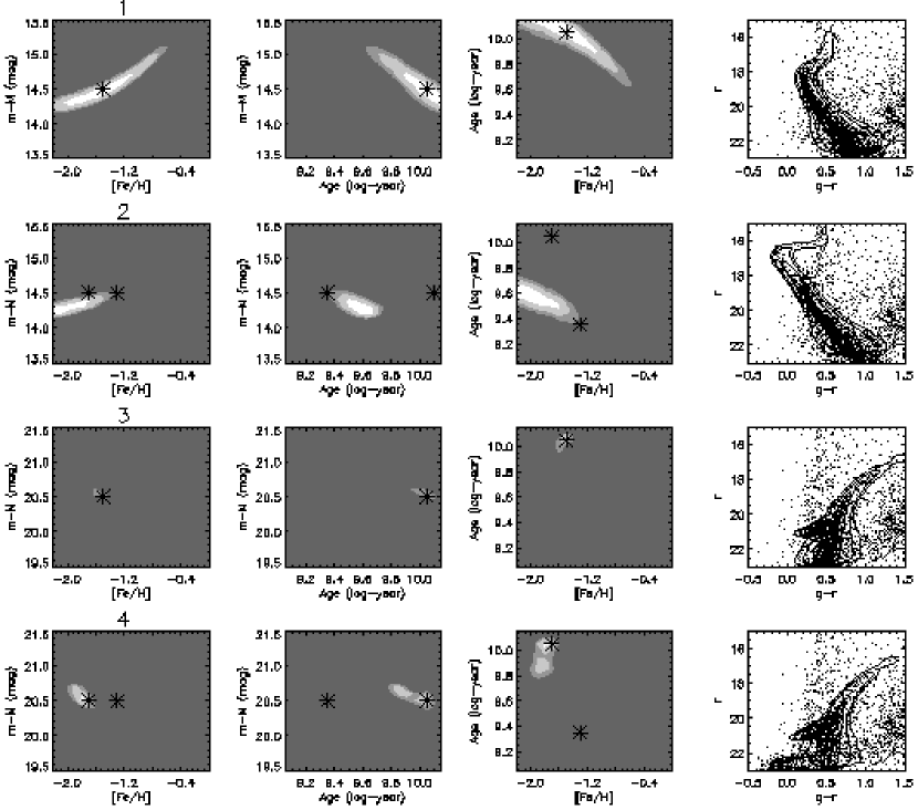
Figure 4.— Contour plots of the single component fitting results for the artificial CMDs. From left to right, the columns show: distance vs. metallicity; distance vs. age; age vs. metallicity; the CMD with the best-fit single component model in contours. The grey-scale contours show the regions in parameter space that are within 1$\sigma$, within 2$\sigma$, within 3$\sigma$ and outside 3$\sigma$ of the best-fitting single component model, going from white to dark gray. Input values for the artificial stellar populations (see also Table 1) are indicated by asterisks.

Using the new distance solution option of MATCH we solve for the SFH of the artificial CMDs again while fixing the metallicity to a single, uniform value. The same age bins are used as for the SFH fits described above, and a distance range of 3.0 is probed with 0.1 magnitude resolution. Including the “control field”, 271 partial CMDs are used in these fits. The fits are done at three different values of the metallicity: [Fe/H]$=-$1.6, $-$1.5, and $-$1.4 to probe the uncertainties. Figure 5 shows the resulting SFHs in relative SFRs and distance determinations.

Figure 5.— Star formation histories and distances for the artificial CMDs from the “distance solution” mode. The columns on the left and the error bars are as in Figure 3. In the columns on the right now the SFR-weighted average distance is plotted for the age bins with significant star formation. Dashed lines indicate the actual input distance for the artificial CMDs.

The SFHs in Figures 3 and 5 show that the software succesfully recovers the single burst in CMDs 1 and 2, and the two distinct episodes of star formation in CMDs 3 and 4. Some bleeding of star formation in adjacent bins will occur even when the fitted age bins exactly match the input SFH (Dolphin, 2001). Therefore it is to be expected that this also happens here, since the duration of the input star forming episodes do not match any age bins perfectly. It should be noted that the error bars in the SFHs represent the range of SFRs encountered in each age bin within the three fits on which the SFHs are based, which means that the errors between adjacent bins are correllated. For example, in the SFH of CMD 4 in Figure 3 the two bins at ages of 2 to 4 Gyr are not independent; when the SFR in one of them is low, it is high in the other. That the age found for the young population in CMD 4 in Figure 5 is the natural result of the metallicities in the fit being lower than the actual metallicity of the younger population. In all cases, the average metallicities and distances found in Figures 3 and 5 agree well with the input values.

Turning to the SC fits in Figure 4, we see that for CMDs 1 and 3, the input properties (indicated by stars) are recovered very well. Because there is a degeneracy between distance, age and metallicity when only the MS and MSTO are seen, the properties of CMD 1 are, however, constrained more poorly than for CMD 3. Since the SC fits use a single model population, the results for CMDs with multiple populations, such as CMDs 2 and 4, cannot be expected to properly recover the properties of all stars. Rather, the population representing the majority of stars in the CMD will have the strongest weight. This is clearly visible in the SC fitting results for CMD 4, that recover the properties of the older population, that dominates the star counts in the RGB and HB. For CMD 2, however, the upper MS and MSTO of the younger population has such high S/N that this population does influence the SC fits significantly and the favored age is relatively young ($\sim$4 Gyr). This shows that for high S/N CMDs with a complex stellar population make-up, the SC fits is not well suited; they were, however, developed for application to low S/N CMDs.

What distinguishes these artificial CMDs from the real data, is that the artificial stellar populations are based on the exact same isochrones, IMF, and photometric error and completeness model as used by MATCH. Inaccuracies in any of these will degrade the fit results one obtains for real data compared to the results for the artificial data.

3. Tests on globular clusters

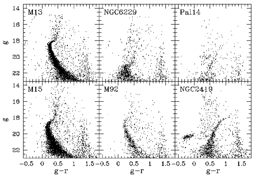
Figure 6.— Color-magnitude diagrams (CMDs) from SDSS DR5 data for the six globular clusters with independently determined population parameters, used to test the CMD-fitting software.

Table 2Globular cluster properties

Cluster	R☉ (kpc)	m-M (mag)	[Fe/H] (dex)	Age (Gyr)	$<E(B-V)>$
M 13	7.7, 7.5a)	14.38, 14.43	$-$1.54	12a)	0.019
M 15	10.3, 10.0b)	15.37, 15.0b)	$-$2.26	13.2b)	0.11
M 92	8.2	14.6	$-$2.28	14c,d)	0.025
NGC 2419	84.2, 98.6e)	19.63, 19.97e)	$-$2.12	14e)	0.060
NGC 6229	30.4	17.44	$-$1.43, $-$1.1f)	$\sim$11.5g)	0.023
Pal 14	73.9	19.34	$-$1.52	$\sim$10h)	0.035

Note. — Values are from Harris (1996), except for: a) Grundahl et al. (1998); b) McNamara et al. (2004); c) Pont et al. (1998); d) Grundahl et al. (2000) ; e) Harris et al. (1997); f) Borissova et al. (1999); g) Vandenberg (2000); h) Sarajedini (1997)

Globular clusters are ideal test cases for the SDSS implementation of MATCH since in most of them their stars have been found to be of a single age and nearly single metallicity. Here we will use six GCs present in the SDSS data to test how well MATCH, using the isochrones from Girardi et al. (2004), can recover their known population properties. The systems in question, M13 (catalog ), M15 (catalog ), M92 (catalog ), NGC 2419 (catalog ), NGC 6229 (catalog ), and Pal 14 (catalog ), cover a large range in distance, background contrast (i.e. ratio of member stars versus field stars) and have metallicities between [Fe/H]$=-2.3$ and $-1.3$ dex. For the following tests, all stars within a 5^∘$\times$5^∘  field centered on each GC were obtained from the SDSS catalog archive server (CAS). It should be noted that in the cases of M15, M92 and NGC 2419 these fields were not completely covered by the DR5 footprint. Flags were used to exclude objects with poor photometry and all stars were individually corrected for foreground extinction using the correction factors provided by DR5 and based on the maps by Schlegel et al. (1998). Any contamination of the samples of stars obtained by misclassified galaxies or other contaminants do not pose problems for our analysis because of the use of control fields that should contain the same populations of these contaminants. “Control field” CMDs were constructed from all stars outside a radius of 0.5^∘  from the center of each GC. “Target fields” were constructed by selecting stars within a certain radius from the center. The radii used for M13, M15, M92, NGC 2419, NGC 6229, and Pal 14 are 0.25^∘, 0.2^∘, 0.25^∘, 0.15^∘, 0.15^∘, and 0.1^∘, respectively. These radii are similar to the tidal radii of the GCs but are not strictly related to them, since in all clusters – and especially in the densest (M13 and M15) – the SDSS photometry in the central parts is missing due to the high degree of crowding. With the radii used, a significant number of field stars is present in each target CMD, so that MATCH has a good handle on the proper scaling of the control CMD.

The SDSS CMDs of the GCs are shown in Figure 6 and their previously measured parameters (distance, age, [Fe/H]) are listed in Table 2; the mean reddening $E(B-V)$ in magnitudes according to the Schlegel et al. (1998) maps in the target area for each GC is also listed in the table. The GCs in the three top panels in Figure 6 have metallicities of around [Fe/H]$=-1.5$ dex, and the GCs in the lower panels are more metal-poor ([Fe/H]$<-2.0$). For the more nearby systems (M13, M15, M92 and NGC 6229) the main CMD features that will drive the fits are the main sequence (MS) and main sequence turn off (MSTO); for the more distant systems (NGC 2419 and Pal 14) only the red giant branch (RGB) and horizontal branch (HB) are observed. Pal 14 in particular represents the case of a very sparsely populated system with high contamination from field stars.

In the following subsections, we discuss the results of applying MATCH to these GCs in the four different modes described in section 2.3. In fitting the CMDs of these objects we will use a color range of $-0.5<g-r<1.5$, and limit the magnitude range to $g<22.5$ and $r<22.0$; the color cut includes the MSTO and the tip of the RGB, but excludes a large fraction of the numerous low-mass foreground stars. For all the fits in this section we will assume a slope for the stellar initial mass function that is close to Salpeter; the binary fraction is assumed to be 0.1, in line with recent observational and theoretical evidence for low binary fractions in globulars (e.g., Ivanova et al., 2005; Zhao & Bailyn, 2005).

3.1. Star formation histories

Figure 7.— Star formation histories and age metallicity relations for the six globulars obtained by using MATCH in its “standard” mode (fitting for age and metallicity distributions at a given distance). Star formation rates are shown relative to the average star formation rate over the entire age range. Error bars along the age axis show the width of each age bin, while the error bars along the y-axis show the range of star formations in the age bin at the three different distances for which a fit was done and the uncertainty in the metallicity in each age bin. Metallicities are only shown for bins with significant star formation. The dashed lines in the right panels indicate the literature values for the metallicity from Table 2.

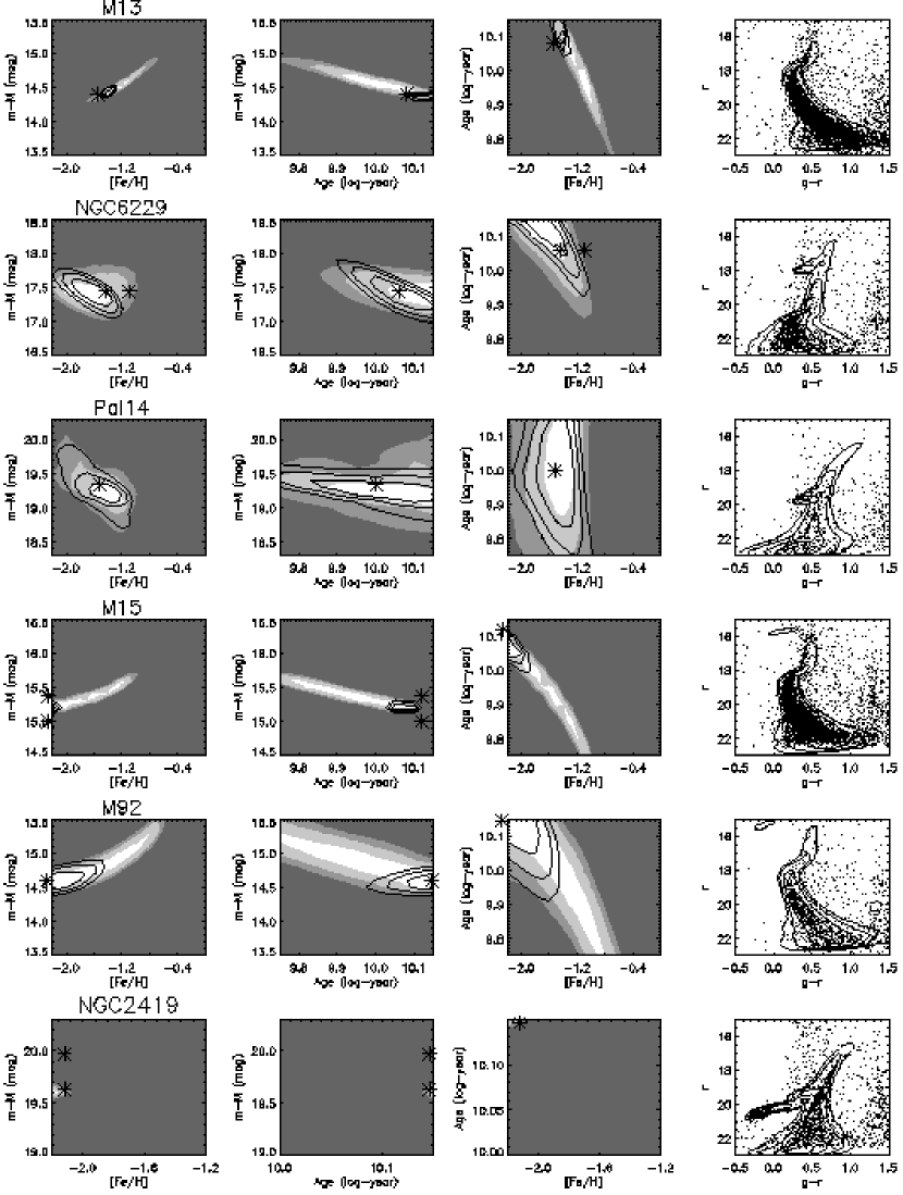
Figure 8.— Comparison of single component population parameters from SDSS and MATCH versus their literature values for the six globulars. The columns show (from left to right): distance vs. metallicity; distance vs. age; age vs. metallicity; the color-magnitude diagram with the best-fit single component model in contours. The grey-scale contours show the regions in parameter space that are within 1$\sigma$, within 2$\sigma$, within 3$\sigma$ and outside 3$\sigma$ of the best-fitting single component model, going from white to dark gray. The solid line contours are for the case in which one of the parameters is fixed to its best-fit value, i.e. age for the left-most, metallicity for the middle-left, and distance for the middle-right columns. Literature values for the parameters are indicated by asterisks.

To measure the SFH and AMR of the clusters we run MATCH fits with nine age bins and twelve metallicity bins. Because the isochrones are spaced more evenly in log $t$ than in $t$, the age bins are defined to have equal width in log $t$, with the oldest running from 10.0 to 10.2 (10 Gyr to 15.8 Gyr) and the youngest from 8.6 to 8.8 (400 Myr to 630 Myr). The metallicity bins cover the range from [Fe/H]$=-$2.4 to 0.0 in twelve bins of 0.2 dex width. Together with the control CMD this yields 109 model CMDs for each GC. The fitting software then finds the linear combination of these model CMDs that best fits the observed CMD. Each object is fit several times with slightly different fixed distances to determine the impact of distance errors on the recovered solutions. In the cases of M15 and NGC 2419, where values from the literature for the distance modulus are quite discrepant, we run fits for distance moduli of 15.0 to 15.4 (M15) and 19.6 to 20.0 (NGC 2419) in 0.1 magnitude steps. For the other clusters we run three fits each, one at the literature value and at 0.1 magnitude further and nearer.

Figure 7 shows the results of these fits, with the fractional SFR as a function of time in the left column, and the metallicity as a function of time in the right column. Metallicities are only plotted for age bins with a significant SFR. The plotted SFR for a given age bin is the average of the values given by the fits at the different distances, with the error bars showing the complete range of SFR values found. The metallicity in a bin is the average of the fits weighted by the SFR, and the error bars correspond to the standard deviation.

Looking at the three intermediate metallicity GCs in the top half of Figure 7 we see that in all cases MATCH infers a purely old ($>$7 Gyr) population, as expected. For M13 and NGC 6229 practically all stars are found to be older than 10 Gyrs; some bleeding into the second oldest age bin is always likely to occur, cf. Section 2.4 and Dolphin (2001). In the case of Pal 14 the SFR is found to be constant over the two oldest age bins, but this only confirms the age estimate of $\sim$10 Gyr (Sarajedini, 1997), which implies that star formation would likely have been spread over these two bins. The intermediate metallicities of M13, NGC 6229 and Pal 14 are reproduced well and our recovered values are within 0.1 to 0.2 dex of the literature values. For NGC 6229 our fits favor the slightly lower metallicity from Harris (1996) rather than the higher value from Borissova et al. (1999).

Turning to the bottom half of Figure 7 with the three metal-poor clusters, we see that here also the results are consistent with a purely old population, although the SFHs of M15 and NGC 2419 show a non-zero SFR in a few younger age bins. In the case of M15 this is due to the blue horizontal branch (BHB) stars that are not properly reproduced by the theoretical isochrones, causing the code to fit them as a younger turn-off. This demonstrates that CMD fitting results always need to be looked at in detail in order to understand their implications. The age distribution in NGC 2419 is not very well constrained because no MSTO is present in the CMD. The metallicities of M15 and M92 are recovered well for the old stars. While the estimated metallicity of $-$1.9 for NGC 2419 is on the high side, for these metal-poor GCs the recovered metallicities are within 0.2 dex of the literature values.

Figure 9.— Star formation histories and distances for the six globulars obtained by using MATCH in the distance solution mode (Section 2.3.2). As in Figure 7 star formation rates are shown relative to the average star formation rate over the entire age range and horizontal error bars show the width of the age bins. Vertical error bars indicate the range of star formation rates encountered at the three different metallicities for which a fit was done, and the uncertainty of the distance. The dashed lines in the right panels indicate the distance values from the literature (see Table 2).

3.2. Single component fitting

Figure 10.— MATCH analysis of a composite CMD: a) CMD of the globular M 13. b) CMD for the globular NGC 6229. c) combined CMD of the globulars M 13 and NGC 6229. d) average result of the three distance solution fits to the CMD in panel a), showing the number of stars in each age-distance bin; the M 13 stars are fit by the oldest age bins around m-M=14.4 magnitudes. e) as in d) but for the CMD in panel b); the NGC 6229 stars are fit by the oldest age bins at m-M=17.2 and 17.4 magnitudes. f) as in d) and e) but for the fits to the combined CMD in panel c); both the ages and distances of the two distinct populations are correctly recovered.

As described in section 2.3.3 above, in the Single Component (SC) fitting mode an individual model CMD is fit to the data together with the control CMD, rather than a whole set of models. The results therefore provide information on the characteristic properties of the dominant stellar population in the CMD. We sample the 3D parameter space of distance, age and metallicity by using one of nine age bins, one of 21 distance bins, and one of 23 metallicity bins. The age bins have a width of 0.1 log-years, going from 10.1-10.2 log-years (12.5 Gyr to 15.8 Gyr) to 9.7-9.8 log-years (5 Gyr to 6.3 Gyr) in steps of 0.05 log-years. This age range more than suffices for these GCs. We use a distance modulus range of two magnitudes centered on the literature value with a resolution of 0.1 magnitude. Metallicity bins are centered at [Fe/H]$=-$2.2 to 0.0 with an inter-bin distance of 0.1 dex and a width of 0.2 dex.

After matching each of the 4347 SC options to each GC and determining the expected variance in the goodness-of-fit parameter $Q$, we take the best fit as our measurement and compare the other fits with respect to these best values. The resulting likelihood contour plots for metallicity, distance and age measurements are shown in Figure 8. Note that in these contour plots, the third parameter is unconstrained, rather than fixed at its known value. If the third parameter would be kept fixed, the contours would shrink significantly. In general the agreement with the literature values (indicated with asterisks in Figure 8) is very good. The small offset for M13 is most likely due to inaccuracies in the isochrones, which illustrates the added uncertainty in CMD fitting results that depend on a single set of theoretical isochrones. Our distance modulus measurement from the SC fits for M15 lies exactly in between the two literature values, while for NGC 2419 our results clearly favor the smaller distance value from Harris et al. (1997). From the two metallicity determinations in the literature for NGC 6229, the fit results agree significantly better with the lower metallicity of [Fe/H]$\sim-$1.4 dex. In some cases, it looks as if the peak of the likelihood lies outside of the parameter space probed, at lower metallicities or older ages. Unfortunately, these limits of the parameter space are dictated by the parameter range of the available isochrones.

Also shown in the right column of Figure 8 are the observed CMDs of the GCs, with contours representing the model populations. In most cases we used the literature parameters for these models, except for M15, where we chose a distance modulus of 15.2, the mean of the two different available values. For NGC 6229 and NGC 2419 we use the literature metallicities and distance moduli that best correspond to our results. The agreement of model and data is generally acceptable, although inaccuracies, especially in the sub-giant branch, can be seen in M13 and M15.

Important to note is the influence of the degeneracies between age, distance, and metallicity. For the nearby systems, M13, M15 and M92, where the fit is driven by the MS, there is a clear distance-metallicity covariance; the left-most panels in Figure 8 show that the distance estimate increases with increasing metallicity. For the distant GC Pal 14, where the fit is driven by the RGB, the covariance is the other way around. Another important, yet not wholly surprising, point is that higher S/N in the CMD features results in much tighter contours, illustrated by the fact that M13, M15 and NGC 2419 give the best constrained results. NGC 2419 has the additional advantage that the well-populated HB provides a very strong constraint on the distance, making this system the best-constrained of the lot.

3.3. Distance solutions

As mentioned in Section 2.3.2, we explore fits for different distances and different ages, with the metallicity linked to the age. The result of each fit is a SFH with a (potentially different) distance for each age bin; differing distances for different sub-populations are not astrophysically relevant for globular clusters, but serve as a test case. For fitting the GCs it seems reasonable to use the same metallicity in all age bins. We use the same nine age bins as in Section 3.1. In distance space we use a distance modulus range of three magnitudes centered on the known distance of each system with a resolution of 0.1 magnitudes, giving a total of 31 distance bins. For each GC we carry out three fits with different metallicities, centered on the literature values (see Table 2) with offsets of 0.1 dex. For NGC 6229 we assume the lower metallicity value [Fe/H]$=-$1.43, which is favored by our SFH and single component fitting results.

In Figure 9 we present the age-distance distributions that result from these fits. Compared to the fits in section 3.1 the number of free parameters per fit is the same, with now metallicity fixed instead of distance. Thus, in general similar quality SFHs should be expected, although not necessarily exactly the same. While in the “standard” SFH fits the star formation within an age bin can be spread over several metallicity bins, it can now be spread over several distance bins. These spread will translate differently into the color-magnitude plane, and therefore can result in differences between the SFHs in Figures 7 and 9.

As in Figure 7 all GCs are found to have a single peak in their SFR in the oldest age bin, in some cases with some bleeding into the adjacent bin. The extension of the SFH of Pal 14 to more recent times has large uncertainties and is not significant. It should be taken into account that the exact age of this system is difficult to constrain with SDSS data, since the MSTO is not present. Interesting to see is that M13 and M92 show almost no bleeding into the second oldest age bin here, while they did in Figure 7; for M15 and NGC 6229 the exact opposite is the case. Apparently, the former are fit better with some distance spread, while the latter benefit more from a metallicity spread. This does not necessarily reflect an actual distance or metallicity spread, but rather shows that inaccuracies in the isochrones are sometimes better accounted for one way and sometimes another way.

The distances we find for the oldest age bin, and therefore for the majority of the stars, show very good agreement with the literature values. Comparing Figures 7 and 9 shows that the SFHs obtained when fixing either the distance or the metallicity are very similar.

The main motivation for enabling this distance fitting mode was, however, not to analyze single-distance systems, but to be able to cope with cases where stars are located at different distances (cf. Canis Major, de Jong et al., 2007). To demonstrate this application, we combine the CMDs of M13 and NGC 6229, resulting in a CMD containing two populations with similar metallicities and ages, but located at significantly different distances. The CMDs of M13, NGC 6229 and the combined CMD are shown in panels a), b) and c) of Figure 10. We run distance solution fits to these CMDs in the same way as before, with the same age bins, but now using a larger distance modulus range, from 12.0 to 19.0 magnitudes with a resolution of 0.2 magnitudes. Three fits are run, for uniform metallicities of [Fe/H]$=-$1.4, $-$1.5, and $-$1.6. We include also a control CMD in the fit which is the control CMD of M 13; since M 13 and NGC 6229 are only 10 degrees apart and at similar Galactic latitudes, this gives good results. The averaged best-fitting distributions of stars over the grid of age and distance bins are shown in panels d), e) and f) of Figure 10. Both ages and distances of the two populations are recovered extremely well, with all stars in the oldest age bin ($>$10 Gyr), M13 stars centered at a distance modulus of 14.4 and NGC 6229 stars at a distance modulus of 17.4. Moreover, the result for the combined CMD is almost exactly the sum of the results for the individual CMDs, clearly illustrating the power of MATCH to decompose more complex CMDs.

3.4. Over-density detection

Figure 11.— Stellar overdensity detection using MATCH: each panel shows the fit quality improvement, d$Q$, between fitting only a control field and fitting a control field plus stellar population model to the CMDs of 20″$\times$20″regions around the six globular clusters. The fields plotted are 5^∘$\times$5^∘fields centered on the globulars with right ascension along the x-axis.

The final application we describe and test here is aimed at algorithmically detecting stellar populations which are confined to a limited distance and area on the sky, i.e. that form “overdensities”. Of course, the GCs used in this section are very obvious stellar overdensities and should be detected at very high S/N. Following the approach described in section 2.3.4 we define a grid of 20′$\times$20′  boxes in each 5^∘$\times$5^∘  field that was obtained from the SDSS catalog server, with the central box centered on the GC. The CMD of each box is fit with the control field CMD and with the control field plus a simple population model. For each GC we use a model with the appropriate distance, age and metallicity. Figure 11 shows the difference in the goodness-of-fit parameter $Q$ between the two fits for areas around each GC. Note that for M15 and M92, the 5^∘$\times$5^∘  field is not completely observed by SDSS. Clearly, all GCs produce high peaks in $\Delta Q$. Since $\Delta Q$ is roughly proportional to the number of stars attributed to the population model in the model fit, the objects with the largest numbers of stars produce the strongest detections. Only in the plot for Pal 14 does the vertical scale allow the random variations in $\Delta Q$ to be visible in the area around the object. The S/N of these detections should be measured with respect to this random noise. Using the 216 boxes around the central 9 boxes we obtain an estimate of the rms in $\Delta Q$ from random variations in the CMDs. Negative values of $\Delta Q$ are suppressed because a negative number of stars in a population is unphysical, which has to be taken into account when calculating the rms. Even Pal 14, a rather sparsely populated and distant cluster, is detected with high S/N, as $\Delta Q_{Pal14}/rms_{\Delta Q}\simeq 56$.

4. Application to new Milky Way satellites

In summary, Section 3 has illustrated the robustness and precision with which MATCH can interpret high-quality CMDs in a variety of circumstances. Over the past few years the importance of deep wide-field surveys for the study of the stellar components of the Milky Way galaxy has been demonstrated by 2MASS (e.g., Ojha, 2001; Ibata et al., 2002; Majewski et al., 2003; Brown et al., 2004; Martin et al., 2004) and the SDSS. Specifically, the SDSS has enabled a detailed picture of the Galactic stellar halo (e.g., Belokurov et al., 2006b; Bell et al., 2007) and led to the discovery of at least fourteen previously unknown dwarf galaxies and globulars: Ursa Major I (catalog ) (UMaI, Willman et al., 2005a), Willman 1 (catalog ) (Wil1, Willman et al., 2005b), Canes Venatici I (catalog ) (CVnI, Zucker et al., 2006a), Bootes I (catalog ) (BooI, Belokurov et al., 2006c), Ursa Major II (catalog ) (UMaII, Zucker et al., 2006b), Coma Berenices (catalog ), Canes Venatici II (catalog ), Hercules (catalog ), Leo IV (catalog ), Segue 1 (catalog ) (Com, CVnII, Her, LeoIV, Seg1, Belokurov et al., 2007), Leo T (catalog ) (Irwin et al., 2007), Bootes II (catalog ) (BooII, Walsh et al., 2007), and two very low-luminosity globulars Koposov 1 (catalog ) and Koposov 2 (catalog ) (Koposov et al., 2007a). While these discoveries are important for our understanding of the so-called “missing satellite problem” (e.g., Klypin et al., 1999; Moore et al., 1999), these new systems might also shed new light on the mechanisms of star formation in low-mass halos with small baryon content. Why these systems were only discovered with SDSS data can be explained by their low surface brightness, as shown by Koposov et al. (2007b). Apart from the promise that more systems of even lower surface brightness might be waiting to be discovered by future generations of deep imaging surveys, this fact raises intriguing questions. Do these systems show that star formation can occur under conditions generally considered to be incapable of supporting such activity, or have these systems evolved to their current state through, for example, tidal interactions with the Galaxy? A thorough and systematic study of the properties of these objects is needed to understand their formation and evolution and the possible cosmological implications.

Several groups have been working on photometric and spectroscopic follow-up of the new MW companions in order to constrain their properties. A compilation of these results is given in Table 3. Although individual measurements of properties might be less precise in some cases, the advantage of studying these objects using the SDSS photometry is that this highly uniform dataset allows a systematic approach to the complete set of objects and fair comparisons between them. In the following, we apply our single component (SC) fitting techniques to constrain the overall distances, metallicities and ages of the objects listed in Table 3. We also constrain the SFH of a subset of objects, since the majority contain too few stars to make this a worthwhile exercise. The objects we use are Boo, CVn I, and UMa I because of their relatively well-populated CMDs, and Leo T because of its clearly complex star formation history. For all the fits in this section we assume a Salpeter-like initial mass function and a binary fraction of 0.5, similar to the value for disk stars (Duquennoy & Mayor, 1991; Kroupa et al., 1993).

Figure 12.— Color-magnitude diagrams from SDSS data for twelve recently discovered Milky Way satellites. The dashed line in the panel for Leo T indicates the separation between the red and blue parts used in the single component fitting analysis (see Section 4.1.1).

Table 3New MW satellite properties

Object	R☉ (kpc)	m-M (mag)	[Fe/H] (dex)	$r_{h}$	$M_{V}$ (mag)
Bootes I	60$\pm$6	18.9$\pm$0.2, 19.1$\pm$0.1a), 19.0$\pm$0.1b)	$\sim$-2, $\sim$-2.5c), $\sim$-2.1d)	12′.8$\pm$0′.7	-5.8$\pm$0.5
Bootes II	60$\pm$10	18.9$\pm$0.5	$\sim$-2	4′$\pm$2′	-3$\pm$1
Canes Venatici I	220$\pm$20	21.75$\pm$0.20	$\sim$-2, -2.5 – -1.5e), -2.0d), -2.09f)	8′.5$\pm$0′.5	-7.9$\pm$0.5
Canes Venatici II	150$\pm$15	20.9$\pm$0.2	-2.3f)	$\sim$3′.2	-4.8$\pm$0.6
Coma Berenices	44$\pm$4	18.2$\pm$0.2	$\sim$-2, -2.00f)	$\sim$5′.5	-3.7$\pm$0.6
Hercules	140$\pm$13	20.7$\pm$0.2	-2.27f)	$\sim$8′.2	-6.0$\pm$0.6
Leo IV	160$\pm$15	21.0$\pm$0.2	-2.3f)	$\sim$3′.4	-5.1$\pm$0.6
Leo T	$\sim$420	$\sim$23.1	$\sim$-1.6, -2.3f)	$\sim$1′.4	$\sim$-7.1
Segue 1	23$\pm$2	16.8$\pm$0.2	-	$\sim$4′.5	-3.0$\pm$0.6
Ursa Major I	$\sim$100	$\sim$20	$\sim$-2, -2.2d), -2.1f)	$\sim$7′.8	$\sim$-6.5
Ursa Major II	32$\pm$5	17.5$\pm$0.3	$\sim$-1.3, -1.6d), -2.0f)	$\sim$12′	-3.8$\pm$0.6
Willman 1	38$\pm$7	17.9$\pm$0.4	$\sim$-1.3, -1.6d)	$\sim$1′.9	$\sim$-2.5

Note. — Values are from the respective discovery papers (see text), unless otherwise indicated: a) Dall’Ora et al. (2006); b) Siegel (2006); c) Muñoz et al. (2006); d) Martin et al. (2007a); e) Ibata et al. (2006); f) Simon & Geha (2007)

4.1. Fitting methods and results

4.1.1 Single component fits

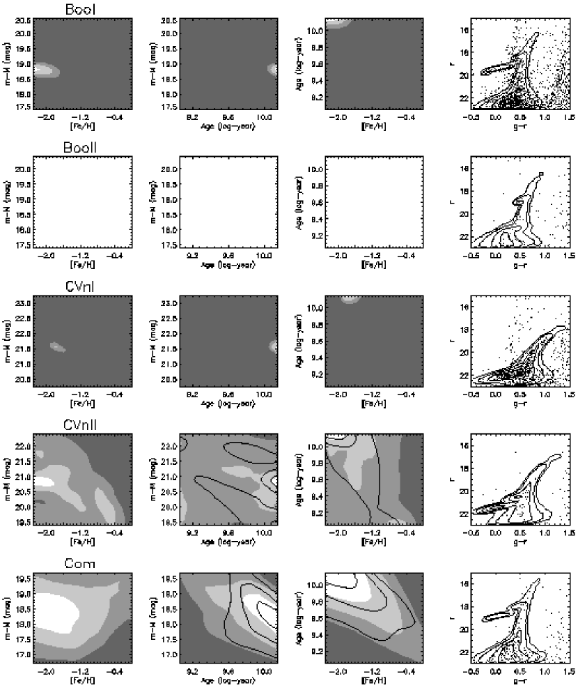
Figure 13.— Population properties of newly discovered Milky Way satellites: the panels show single component fitting results for Boo I, Boo II, CVn I, CVn II and Com, with the columns showing (from left to right): distance vs. metallicity; distance vs. age; age vs. metallicity; and the color-magnitude diagram with the best-fit single component model in contours. The gray-scale contours show the regions in parameter space that are within 1$\sigma$, within 2$\sigma$, within 3$\sigma$ and outside 3$\sigma$ of the best-fitting single component model, going from white to dark gray. The solid line contours are for the case in which one of the parameters is fixed to the literature value (i.e. age for the left-most, metallicity for the middle-left, and distance for the middle-right columns), where available.

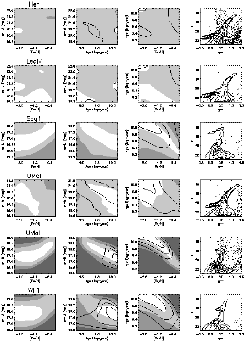
Figure 14.— Same as Figure 13, but for Her, Leo IV, Seg 1, UMa I, UMa II and Wil 1.

As for the GCs we obtained data in 5^∘$\times$5^∘  fields around each object from the SDSS CAS as outlined in section 3. For the target CMDs we used the stars within one half-light radius ($r_{h}$, Table 3) from the center (with a minimum of 3′), with all stars outside a radius of 60′  used for the control CMDs. Figure 12 shows the target CMDs for the twelve objects. In all cases except Leo T a color range of $-0.5<g-r<1.5$ is used for the CMD fits. The population parameter space we sample consists of 12 age bins, 24 metallicity bins and 31 distance bins. The age bins have a 0.1 log-year width and separations of 0.1 log-year, with the oldest running from 10.1–10.2 log-years (12.5 Gyr to 15.8 Gyr) and the youngest from 9.0–9.1 (1 Gyr to 1.26 Gyr). Metallicities run from [Fe/H]=$-$2.3 to 0.0 in steps of 0.1 dex, and each metallicity bin has a width of 0.2 dex. The range in distance modulus probed is 3 magnitudes wide, with a resolution of 0.1 magnitudes, and is centered on the literature value for each object.

For Leo T we use a slightly different approach. The group of blue stars in the CMD is too bright and does not have the right morphology to be interpreted as HB stars belonging to the same population as the RGB stars. This means there are two populations present in two different parts of the CMD, with the RGB corresponding to the old population and the stars at $g-r\lesssim$0.3 to a much younger population. As demonstrated in Section 2.4, in such a case the SC fits will give very poor results. However, since the two populations in Leo T are only present on one side of the $g-r\simeq 0.3$ line, they can be easily separated. Thus, to determine the properties of the two populations separately we divide the Leo T CMD into a red (-1.0$<g-r<$0.3) and a blue (0.3$<g-r<$1.5) part and fit these separately. The red part of the CMD is fit with the same parameter space as the other objects. For the blue part the same metallicities and distance moduli are probed, but a younger set of age bins is used. Here we use nine bins, the four oldest of which have a width of 0.1 log-years centered on 9.05, 9.15, 9.25 and 9.35; the five youngest have a width of 0.2 log-years centered on 8.1, 8.3, 8.5, 8.7 and 8.9 log-years.

In Figures 13 and 14 the SC fitting results for the new MW satellites, except Leo T, are presented. The right-most panels show the CMD of each object again, with the best-fit SC model overplotted as contours. Monte Carlo runs were used to determine the values of $\sigma$. Except for Boo I and CVn I, solid contours are shown for the case of a fixed metallicity or age, where such a measurement is available in the literature. Figure 15 shows the same results for the red and blue part of the Leo T CMD. The fact that low S/N hinders a robust determination of the population properties provides a serious problem for the majority of the targets. Although for most objects a finite region of parameter space lies within 1 $\sigma$ from the best fit (the white area in the contour plots), reasonable measurements of any individual parameter can only be obtained for Boo I, CVn I, CVn II, Com and Her. Especially for Boo II, Leo IV and Leo T, parameters are very poorly constrained, and $Q$ space shows a complicated morphology with multiple minima.

Figure 15.— Same as Figure 13, but for the red part ($g-r>0.3$) of the Leo T CMD (upper panels) and for the blue part (lower panels).

4.1.2 Star formation histories

To constrain the SFHs of Boo I, CVn I, Leo T and UMa II we follow the same approach as before for the GCs. A grid composed of nine age bins and twelve metallicity bins is used, the age bins going from 10.2 to 8.4 log-years with an 0.2 log-year width, and the metallicities from [Fe/H]=-2.4 to 0.0 with a 0.2 dex width. A fit is done at three different distance moduli, 0.1 magnitude apart, with the middle value equal to the literature value. The resulting SFHs and AMRs are plotted in Figure 16.

Figure 16.— Same as Figure 7 but showing the star formation histories and age metallicity relations for Boo, CVn I, Leo T and UMa II.

4.1.3 Object detection

As with the GCs, we also test our overdensity detection scheme, described in Section 2.3.4, on these new Milky Way satellites. The 5^∘$\times$5^∘  field centered on each object is divided in a square grid of 225 20′$\times$20′  boxes, the CMDs of which are fit both with a control field and with the control field plus a single component population model. As the control field the whole 5^∘$\times$5^∘  field is used. For the SC model we consider two cases. First we use a typical old population model, with age range 10.0 to 10.1 log-year and [Fe/H]$=2.0$ at the best-fit distance obtained with the SC fits from Section 4.1.1. Second we use a model corresponding to the best-fit properties obtained for each object. The former case serves to simulate a realistic search of all SDSS data for unknown stellar overdensities. When performing such a search, an old, metal-poor model would be a likely choice since most MW satellites are dominated by such populations. Another factor that would influence the results of a search for unknown stellar overdensities is the size of the box used. As a test, we also did the same exercise using different box sizes for Boo I. In addition to the 20′$\times$20′  boxes, we also used 40′$\times$40′  boxes and 1^∘$\times$1^∘boxes. To enable the use of these coarser grids, we retrieved a larger, 10^∘$\times$10^∘  field from the SDSS DR5 archive centered on Boo I.

In Figure 17 we present the results of the fits with the fine-tuned stellar population models to the twelve objects. Each panel shows the improvement in the goodness-of-fit, $dQ$, as function of the position in the field centered on a satellite. Figure 18 shows the resulting $dQ$ for the three different box sizes in a 10^∘$\times$10^∘  field centered on Boo I. The significances of all detections, expressed in $dQ/rms$, are listed in Table 4.

Figure 17.— Using MATCH to detect or verify stellar overdensities: Each panel shows (for one of the Milky Way satellites) the difference in fit quality, $dQ$, between fitting only a control field and fitting a control field plus SC model to the CMDs of a grid of boxes on the sky. For this, the 5^∘$\times$5^∘  fields centered on each target were divided in 225 20′$\times$20′  boxes. A high value of $dQ$ indicates a large improvement and the presence of a large number of stars that are well-fit by the SC model.

Figure 18.— Overdensity detection applied to Boo I using different spatial resolutions. A 10^∘$\times$10^∘  field centered on Boo I is divided into 20′$\times$20′  (left panel), 40′$\times$40′  (middle panel), and 1^∘$\times$1^∘  (right panel) boxes. The fit improvement, $dQ$, between a pure control field fit and a control field plus SC model fit, is plotted as function of position on the sky.

Table 4Detection significance for new Milky Way satellites

Object	Old $dQ/rms$	Fine-tuned $dQ/rms$
Boo Ia)	106.9	121.6, 58.2, 27.8
Boo II	0.86	0.93
CVn I	447.7	589.4
CVn II	2.61	13.3
Com	57.5	53.9
Her	15.2	28.2
Leo IV	13.8	38.2
Leo T	5.8	11.3
Seg 1	9.9	7.8
UMa I	12.9	11.2
UMa II	1156.2	865.3
Wil 1	48.8	47.8

Note. — a) the three values of $dQ/rms$ for the fine-tuned model fits to Boo I correspond to the box sizes of 20′$\times$20′ , 40′$\times$40′  and 1^∘$\times$1^∘, respectively.

4.2. Discussion

4.2.1 Satellite properties

We have performed a systematic and uniform numerical CMD analysis of the recently discovered MW satellites. How well the properties of an individual object can be determined depends on the number of member stars present in the CMD and the observed CMD features. For some objects, this type of analysis is hard-pressed to provide strong statistical constraints due to the sparseness of their CMDs. In Table 5 we summarize the results of our single component and star formation history fits. The distance moduli, metallicities and ages listed are the unweighted averages of all SC fits that lie within 1 $\sigma$ of the best SC fit and are therefore considered to be acceptable fits. The errors are the standard deviations of the parameter values of these fits, combined with an added systematic uncertainty of 0.1 dex in [Fe/H] and 0.1 mag in distance modulus to account for isochrone uncertainties. In cases where these properties cannot be sufficiently constrained we list the metallicities and ages we get when assuming the distance modulus from the literature, as this is usually the best-determined property. The star formation history results, where available, are summarized in Table 5 by the main star formation episodes. Below follows an object-by-object discussion of these and the star formation history results.

Boo I.— This dwarf spheroidal is relatively nearby at $\sim$60 kpc and an RGB, HB and MSTO are all present in the SDSS data, albeit sparsely sampled. The overall properties can therefore be determined with relatively good accuracy, and the star formation history is the best-constrained of all. Especially the distance of Boo I is very well constrained thanks to the HB which is detected at high S/N due to the absence of field stars at $g-r<$0. The MSTO and slope of the RGB provide constraints on the age and metallicity, respectively. Our distance, metallicity and age measurements agree very well with the findings of other authors based on spectroscopy and deeper imaging data. The star formation history shows one significant epoch of star formation in the oldest ($>10$ Gyr) bin, with no other bins containing a significant SFR. Considering the ability of these fits to distinguish between a single and a multiple component system, demonstrated by the fits to the artificial CMDs in Section 2.4, we conclude, despite the sparseness of the CMD, that Boo I very probably only contains old stars. Thus, our results are consistent with the picture of a purely old, metal-poor stellar population.

Boo II.— The number of Boo II member stars in the SDSS data is very small and traces only the RGB. Unfortunately, the resulting very low S/N combined with the degeneracies between the different parameters make it impossible for MATCH to constrain the stellar population parameters in a statistically significant way. Although Walsh et al. (2007) show that the SDSS CMD of Boo II is consistent with Boo II having similar metallicity, age, and distance as Boo I, The SDSS data alone do not support any significant constraints on any of these properties. The only way to get such constraints is by obtaining deeper follow-up data.

CVn I.— Being the brightest of the twelve objects analyzed here, CVn I has a well-populated RGB and HB. This helps to increase the robustness of the constraints we obtain from the SC fits. Although at the edge of the sensitivity limits of SDSS, the HB enables the determination of the distance. Moreover, the extent of the HB to very blue colors requires the stars in CVn I to be both old and metal-poor. This constraint on the metallicity is further enhanced by the slope of the RGB. Together, the extended HB and RGB thus can provide robust constraints on the properties of the dominant stellar population. The distance modulus we find is slightly smaller than that found in the literature, but not significantly so. The metallicity of [Fe/H]=-1.8$\pm$0.2 falls nicely within the range of metallicities observed by Ibata et al. (2006). Although an age of 14$\pm$2 Gyr fits the CMD best, the star formation history shows two peaks. The oldest star forming episode in the 10-16 Gyr bin is dominant in terms of the number of stars and drives the SC fits, but the peak in the 2.5-4 Gyr bin is equally significant. For the old stars the metallicity is found to be close to [Fe/H]=-2, while the younger stars have metallicities around [Fe/H]=-1.5. It should be noted that the young population found here is not caused by the algorithm attempting to fit BHB stars, as is the case for M15 in Figure 7. Stars belonging to this young population only appear in the regions of the CMD where the RGB and the red part of the HB are located. The presence of two populations is therefore purely based on the RGB morphology and the density of stars along the HB. This detection of an old and intermediate age population with these metallicities confirms the findings of Ibata et al. (2006) and Martin et al. (2007b). Furthermore, Zucker et al. (2006a) note the presence of a carbon star very close to the center of CVn I and its heliocentric radial velocity of 36$\pm$20 km/s is consistent with the radial velocities that Ibata et al. (2006) and Simon & Geha (2007) measure for CVn I, making it is likely that this star belongs to the CVn I dwarf. Since carbon stars are often of intermediate age, this is another indication of the presence of an intermediate age population in this system.

CVn II.— Although very faint and distant, our distance measurement for CVn II is very accurate and in very good agreement with the value from Belokurov et al. (2007) due to the presence of HB stars. From the extension of the HB to very blue colors ($g-r\sim-0.3$) we can infer that the stellar population is both old and metal-poor. Despite the sparseness of the CMD we thus get relatively good constraints on these parameters and we find a metallicity of [Fe/H]$\sim$-2 and a very high age. CVn II thus appears to be a very old and metal-poor object.

Com.— An absence of a clear HB makes constraining the distance of Com difficult and leads to a strong degeneracy between age, distance and metallicity. Similar degeneracies occur for artificial CMD 1 in Section 2.4 and the GC NGC 6229 (see Figures 4 and 7), even though their CMDs are much less sparsely populated. The RGB and MSTO alone do not allow a robust determination of the individual population parameters. As a consequence, the distance modulus we recover has rather large error bars but is consistent with the findings of Belokurov et al. (2007). The SC fits favor an ancient population ($>10$ Gyr) and a metallicity of [Fe/H]$\sim-$2, but also here the uncertainties are large.

Her.— In the case of Her the contamination of the CMD with fore- and background stars is severe, which is due to its location at lower Galactic latitudes compared to the other objects. This high contamination means a low S/N of the CMD features of Her, apart from the HB, which is in the relatively clean part of the CMD at $g-r<0$. Our distance modulus of 20.4$\pm$0.2, which largely is determined by the HB, is somewhat lower than estimated by Belokurov et al. (2007), but is consistent within the error bars. This object too is consistent with an ancient and metal-poor ([Fe/H]$\sim$-2) stellar population. Even though the region of parameter space that lies within 1 $\sigma$ of the best fit values is well constrained, the complete parameter space lies within 2 $\sigma$, which is due to the low S/N of the CMD. These results based only on SDSS data are also consistent with the results obtained by applying the same methods to much deeper $B,V$ photometry from the Large Binocular Telescope (Coleman et al., 2007). In fact, the uncertainties on the values of distance, metallicity and age from the deeper data are very similar to the 1$\sigma$ values we obtain here.

Table 5New MW satellite results

Object	m-M	[Fe/H]	Age	SF episodes
Bootes I (BooI)	18.8$\pm$0.2	-2.2$\pm$0.2	14$\pm$2	$\sim$10-16 Gyr
Bootes II (BooII)	-	-	-	-
Canes Venatici I (CVnI)	21.5$\pm$0.2	-1.8$\pm$0.2	14$\pm$2	$\sim$2-4 Gyr, $\sim$10-16 Gyr
Canes Venatici II (CVnII)	20.8$\pm$0.2	-2.1$\pm$0.3	14$\pm$2	-
Coma Berenices (Com)	18.4$\pm$0.4	-1.9$\pm 0.4$	11$\pm 5$	-
Hercules (Her)	20.4$\pm$0.2	-2.1$\pm$0.2	14$\pm$3	-
Leo IV (LeoIV)	-	-2.1$\pm$0.3	14$\pm$2	-
Leo T (LeoT)	23.1$\pm$0.6	-1.6$\pm$0.6	-	$<1$ Gyr, $\sim$6-10 Gyr
Segue 1 (Seg1)	-	-1.6$\pm$0.5	11$\pm$4	-
Ursa Major I (UMaI)	-	-1.8$\pm$0.4	10$\pm$5	-
Ursa Major II (UMaII)	-	-1.5$\pm$0.5	11$\pm$4	$\sim$2-6 Gyr, $\sim$10-16 Gyr
Willman 1 (Wil1)	17.9$\pm$0.4	-1.6$\pm$0.5	10$\pm$5	-

Leo IV.— The CMD of Leo IV is so sparse that a statistically significant determination of the population properties is not possible based on the SC fits alone. The best fit is given by a population of $\sim$14 Gyr old stars with [Fe/H]=$-$2.2 at a distance modulus of 20.8, but a large number of models gives a goodness-of-fit that is only marginally worse. Assuming a distance modulus of 21.0 (Belokurov et al., 2007), gives the solid contours in the age-metallicity panel for Leo IV in Figure 14. Using this prior, the SC fits allow the age and metallicity to be constrained to 14$\pm$2 Gyr and [Fe/H]$=-$2.1 $\pm$0.3, respectively.

Leo T.— This object is very interesting and differs from the others analyzed here, in that it is the least luminous system known which shows signs of on-going star formation and has HI gas associated with it (Irwin et al., 2007). Because of the presence of two clearly very different populations the SC fitting method is not very well suited. Even when fitting the two populations separately, by dividing the CMD in two distinct parts as we have done, the results are poor, due to the small numbers of stars in each part. Taking the results of the two populations together we find a distance modulus of 23.1$\pm$0.6 magnitudes. Both the old and young populations are best fit with low metallicities, [Fe/H]$\lesssim$-1.5. The star formation history we find (Figure 16) clearly shows two peaks, confirming the presence of two distinct populations. The age of the old population, not well-constrained with the SC fits, is put in the 6.5-10 Gyr age bin. Comparing this with the SFHs of the GCs in Figure 7 and the other SFHs in Figure 16, where in all cases the peak of star formation is in the oldest age bin, this implies that the old population in Leo T is on average younger than the old population in these other objects. The young stars are clearly found in the three youngest age bins, where they are fit as young ($<1$ Gyr) blue loop stars. Irwin et al. (2007) interpreted the nature of these stars similarly.

Seg1.— In Seg 1 only a MS and MSTO are populated in the very sparse CMD. As with the artificial CMD 1 in Section 2.4 and the GCs M13, M15 and M92, where the SC fits also solely relie on the MS and MSTO, strong degeneracies between age, distance and metallicity are expected. Indeed, the contour plots for Seg 1 in Figure 14 show a similar morphology, but due to the sparseness of the CMD with even poorer constraints. This makes any determination of the population properties of Seg 1, based solely on the SC fits, impossible. Even when using the distance modulus from Belokurov et al. (2007) as a prior, the age-metallicity degeneracy prevents strong constraints on these parameters, resulting in very large error bars on the values for Seg 1 listed in Table 5.

UMa I.— This object also has a very sparsely populated CMD. An RGB is readily seen, with some probable HB stars that, however, are too few to produce strong statistical constraints on the distance. Because of this and the usual degeneracies, the significance of the SC fit results is very low, causing all parameters to be poorly constrained. Assuming a distance modulus of 20 (Willman et al., 2005a), our results are consistent with an old ($\sim$10 Gyr) and metal-poor population, but with large error bars.

UMa II.— Although the MSTO of UMa II is well-populated, the scarcity of stars in other parts of the CMD provides problems for this object. There are some RC stars, but the S/N of this CMD feature is not high enough to make for a reliable distance determination. Added to that there are strong degeneracies between the different solutions; similar degeneracies are seen in Section 3 for the GC NGC 6229 where also the MSTO drives the SC fit results. Our results are, however, consistent with previous findings. With a prior on the distance modulus, $m-M=$17.5, the fits agree with the conclusion of Zucker et al. (2006b) that UMa II is not very metal-poor, but seems to have a more intermediate metallicity of [Fe/H]$\sim-$1.5, although the error bars are large (see Table 5). The spectroscopic metallicity measurement from Martin et al. (2007a) is consistent with our value, but the one from Simon & Geha (2007) is more metal-poor, but still consistent within the errors. While the SC fits imply that the majority of stars is likely old, $\sim$11 Gyr, the SFH (Figure 16) hints at more complexity. According to the SFH results, there is a population of very old ($>$10 Gyr) and metal-poor ([Fe/H]$\simeq$-2), as well as a younger ($\sim$5 Gyr), close to solar metallicity population. Since the SC fits measure the average properties, this is consistent with the intermediate metallicity we find there. Zucker et al. (2006b) report that the upper main sequence of UMa II in their deeper Subaru data is wider than expected just from observational errors, one explanation for which could be the presence of a mix of populations. Also in our fit, the double peak results from the width of the MSTO, which is less well-fit by a single-age population. The exact ages and metallicities of the populations should be studied with deeper and spectroscopic data, since the SDSS CMD does not support such detailed conclusions. However, taking our SFH fit and these other results together it does seem likely that UMa II, like CVn I, is a system with a complex star formation history, which might also be (part of) the explanation for the discrepancy between the two available spectroscopic metallicity measurements.

Wil1.— For this system only the MSTO is observed, which is also sparsely populated. This leads to a strongly degenerate solution space, similar to the cases of UMa II and Seg 1. The distance can be determined slightly better here, but the range of distance moduli for which fits within 1$\sigma$ from the best fit can be obtained is still very large: 17.2$<m-M<$18.5. Using the distance modulus from Willman et al. (2005b) (m-M=17.9) as a prior, the fit results imply an old population ($\sim$10 Gyr) with an intermediate to low metallicity ([Fe/H]$\sim$-1.6), but also here the error bars on these numbers are large.

Figure 19.— CMD fitting results for new Milky Way satellites: Left: metallicities from this paper (filled circles) versus absolute magnitude, compared with spectroscopic metallicities from Martin et al. (2007a) (open squares) and Simon & Geha (2007) (open triangles). For clarity, only the error bars on the results from this work are shown. Middle: ages of the satellites versus absolute magnitude. Open circles denote objects for which a full SFH fit was done, and in the cases where two distinct populations were found (CVn I, Leo T and UMa II) both are plotted; filled circles denote objects where the age is only determined from the SC fits. Right: as in the middle panel, the ages are plotted, but now versus distance modulus.

Figure 19 summarizes our results from the MATCH fits to the CMDs for the sample of new Milky Way satellites. In the left panel we plot our metallicity estimates for all objects versus their absolute magnitudes, together with the spectroscopic metallicities from Martin et al. (2007a) and Simon & Geha (2007). Especially for the fainter objects our metallicity estimates are very poorly constrained (Figures 13 and 14) and because of the available isochrones our metallicity range is restricted to [Fe/H]$=-$2.4 at the metal-poor end. In light of this, our photometric results agree remarkably well with the spectroscopic values. Still, care has to be taken when drawing conclusions from these metallicity estimates. We can say at best that we find no indication for a corellation between metallicity and the luminosity of the objects, which is observed for brighter dwarf spheroidals (e.g., Grebel & Guhathakurta, 1999; Grebel et al., 2003). The mean age of the stars versus absolute magnitude is shown in the middle panel of Figure 19. For objects in which the SFH fits showed evidence for two populations, both populations are plotted separately. The right panel shows the inferred ages of the satellites versus distance modulus, to probe possible environmental influences.

Looking at the middle panel of Figure 19 there is no clear evidence for a luminosity dependence of the ability of a dwarf galaxy to form stars recently. Although the two most luminous objects in this sample, Leo T and CVn I, both have young or intermediate age populations, the much fainter UMa II does as well. While the environment might play a role, the right panel of Figure 19 shows no obvious relation between age or the presence of multiple star formation epochs with distance from the sun (since these objects are at high Galactic latitude and at large distances, the heliocentric and galactocentric distances are not significantly different). This is contrary to the trend suggested by van den Bergh (1994) for the brighter Local Group dwarf spheroidals, in which systems with a larger fraction of young or intermediate age stars are systematically more distant.

4.2.2 Satellite detection

Figure 20.— Histogram of the $dQ/rms$ distribution for an empty region of sky of effective area of $\sim$800 square degrees.

Since most of these recently detected objects are intrinsically faint and/or distant, they are of course much harder to detect by any overdensity detection scheme than the GCs. The improvement in the goodness-of-fit, $dQ$, between a fit with a control field only and a control field plus SC model is roughly proportional to the number of stars in the CMD that can be fit by the SC model. This means that the objects with sparsely populated CMDs are the most difficult to detect. Comparing the overdensity detection results in Figure 17 with the CMDs of the objects (Figure 12) confirms this, as Boo, CVn I and UMa II give by far the highest $dQ$. Similarly, the rms noise in $dQ$ increases with increasing numbers of field stars in the CMDs, and at the low S/N end the noise level starts to play an important role. For example, comparing the panels for Boo II and CVn II in Figure 17, which have the same $dQ$ scale, reveals very different noise levels. This can be traced back to the positions of these objects on the sky, with Bootes II lying behind the Sagittarius stream and CVn II in a much ‘cleaner’ region of the halo. The Sagittarius stream also produces a high noise level around Segue 1.

While most objects produce clear peaks in $dQ$, the detectability of several is rather low. For example, CVn II, Leo T, Segue 1 and UMa I have a $dQ$ only a factor of a few higher than the most prominent noise peaks; Boo II is not clearly detected at all. When inspecting the values in Table 4, it turns out that the use of a fine-tuned population model as compared to the generic old, metal-poor model has a varied effect. In some cases the detection significance is improved, in some cases the change has little effect and in a few cases the detectability is actually decreased. In these last cases, even though the peak $dQ$ is the same to or higher for the fine-tuned model, the change in the rms causes the detection to become less significant. This indicates that, while sampling a range of population models would be preferable when doing an overdensity search, a relatively small grid of models will not severely compromise the outcome.

To test the significance of the $dQ/rms$ measure, we tested the overdensity detection scheme on a presumably ‘empty’ patch of SDSS sky with 170^∘$<$RA$<$200^∘and 40^∘$<$Dec$<$65^∘. This patch of sky was divided into 20′$\times$20′  boxes with some overlap, giving a total of 7088 boxes, equalling an effective search area of almost 800 square degrees. A control field (the CMD from the surounding 5^∘$\times$5^∘area) was fit to the CMD of each box, as well as this control field plus a typical old stellar population model with an age bin of 10.0 to 10.1 log-year and [Fe/H]=-2. This was done seven times, with the stellar population model shifted to different distance moduli: 17.0, 18.0, 19.0, 20.0, 21.0, 22.0 and 23.0 magnitudes. Thus, for each box seven values of $dQ/rms$ are obtained, where the rms is obtained from the boxes in the surounding 5^∘$\times$5^∘. The methodology closely resembles the approach used for the MW satellites. Figure 20 shows the histogram of all $dQ/rms$ values for all boxes (solid line), as well as for two individual distance moduli, 18.0 (dotted) and 22.0 (dashed) mag. All three histograms show the same distribution, implying that the noise behaves similarly for all distance moduli. The tail of the distribution extends to $dQ/rms\sim 8$. An inspection of the locations with values higher than 7 reveals no obvious overdensities, implying that this tail is indeed caused by noise. In order to obtain a clean sample of stellar overdensity detections, a $dQ/rms$ threshold of $\sim$9 seems appropriate. This means that when using a sufficiently sampled grid of population models and distances, all new MW satellites would be detected, with the exception of Boo II (cf. Table 4).

The results of the fits to Boo I with different box sizes, listed in Table 4 and shown in Figure 18, illustrate the effect of the spatial resolution of the CMD grid. Here, the detectability is also strongly affected by the rms of the background noise. Since the $dQ$ due to random variations in the field population increases with increasing numbers of field stars, the rms is higher for larger box sizes, favoring the smallest boxes used here. The fact that the $\Delta Q/rms$ decreases roughly by a factor of 2 as we move to larger box sizes is caused by the number of background stars increasing by a factor 4, while the number of Boo I stars in the central box does not change. It is also interesting to note that here the noise is dominated by the Sagittarius stream, which runs accross the lower left corner of the panels in Figure 18. The significance of the detections in Table 4 can be boosted by decreasing the box sizes, especially for the objects with the smallest (projected) size.

5. Summary and conclusions

We have shown that application of MATCH (Dolphin, 2001) to Hess diagrams or CMDs of SDSS data successfully recovers the known stellar population properties of globular clusters (Section 3), within the limitations of the data. This gives confidence that despite inaccuracies in the theoretical isochrones in isolated parts of the CMD, the overall CMD-fitting technique still provides good and trustworthy results. Apart from the standard star formation history fitting method, we have also demonstrated three other ways of applying MATCH to SDSS data:
1) Identifying the best fitting ‘single component’ stellar population, a mode useful for CMDs of very faint or distant objects with limited S/N in their CMD;
2) Fitting the line-of-sight distribution of stars – to keep the fit’s degrees of freedom constant, we fix the metallicity at each age bin; and
3) Algorithmic detection of objects, i.e. of a localized stellar population overdensity in a particular (unknown) direction and at a particular (unknown) distance. This is done by comparing the difference in the goodness-of-fit between a CMD-fit to a control field and a CMD-fit to a control field plus model population.

These tests show that the application of CMD-fitting techniques to wide-field survey data is a very promising endeavor in the light of SDSS and other surveys that will start yielding data over the next few years. Further improvements in software and theoretical isochrones can only increase the use and accuracy of such work. On the basis of these tests and the application to known globular clusters, we have applied our single component fitting technique to twelve recently discovered Milky Way satellites. The sparseness of several of the CMDs of these objects inhibits a robust determination of the population parameters and the best fit solutions are often not unique. In order to obtain good constraints at least some CMD features such as the MSTO, HB and RGB should be observed with sufficiently high S/N. For the least luminous objects this is inherently problematic because of their lack of (evolved) stars. For only four of the satellites, the CMDs had sufficiently high S/N to warrant a star formation history fit.

The results of the population fits to the new Milky Way satellites, summarized in Table 5, are consistent with the individual discovery and follow-up studies. When looking at the sample as a whole, we find that the majority of these objects are likely dominated by old ($\gtrsim$ 10 Gyr) and metal-poor ([Fe/H]$\sim$-2) stellar populations. For Boo, CVn II, Com, and Her the single component fits converge to this picture, and for Boo the full fit of a star formation history also confirms this. Seg 1, UMa I, UMa II, and Wil 1 are not well constrained by the SC fits, but using the distances from the literature as priors, they are also consistent with similar ages and metallicities, although slightly higher metallicities ([Fe/H]$\sim-$1.6) cannot be excluded. The single component fits show CVn I to be old as well, but not extremely metal-poor. However, the SFH reveals the presence of both an old, metal-poor, as well as a younger ($\lesssim$3 Gyr) and more metal-rich population. This is consistent with the findings of Ibata et al. (2006), who detect two kinematically distinct populations in CVn I which differ in age and metallicity, and the detection of a young component by Martin et al. (2007b) in deeper photometry. The SFH of UMa II also shows a peak at an age of $\sim$5 Gyr, which supports suggestion of multiple populations in this object by Zucker et al. (2006b), who find the MSTO width of UMa II to be too large to be explained by photometric errors alone. Finally, in Leo T the presence of two distinct populations is readily seen in the CMD and reproduced in the star formation history. The RGB seen in this system belongs most likely to an intermediate age ($\sim$5-10 Gyr) population with a metallicity of [Fe/H]$\sim$-1.5 to -2, while the blue stars in the CMD are most likely very young ($<$1 Gyr) blue loop stars with similar metallicities. The objects studied here are all intrinsically faint and sparse, and in some cases the population parameters can be constrained only poorly. However, their star formation histories do not appear uniform, nor do all of them appear to be exclusively old and metal poor.

References

- Adelman-McCarthy et al. (2007) Adelman-McCarthy et al. 2007, ApJS, in press
- Aparicio, Gallart & Bertelli (1997) Aparicio, A., Gallart, C. & Bertelli, G. 1997, AJ, 114, 680
- Bell et al. (2007) Bell, E. F., et al. 2007, ApJ, subm., arXiv:0706.0004
- Belokurov et al. (2006a) Belokurov, V., Evans, N. W., Irwin, M. J., Hewett, P. C., & Wilkinson, M. I. 2006a, ApJ, 637, L29
- Belokurov et al. (2006b) Belokurov, V., et al. 2006b, ApJ, 642, L137
- Belokurov et al. (2006c) Belokurov, V., et al. 2006c, ApJ, 647, L111
- Belokurov et al. (2007) Belokurov, V., et al. 2007, ApJ, 654, 897
- Borissova et al. (1999) Borissova, J., Catelan, M. , Ferraro, F. R., Spassova, N., Buonanno, R., Iannicola, G., Richtler, T., & Sweigart, A. V. 1999, A&A, 343, 813
- Brown et al. (2004) Brown, W. R., Geller, M. J., Kenyon, S. J., Beers, T. C., Kurtz, M. J., & Roll, J. B. 2004, AJ, 127, 1555
- Bullock & Johnston (2005) Bullock, J. S., & Johnston, K. V. 2005, ApJ, 635, 931
- Clem (2006) Clem, J. L. 2006, PhD Th., Univ. of Victoria
- Coleman et al. (2007) Coleman, M., et al. 2007, ApJ, subm., arXiv:0706.1669
- Dall’Ora et al. (2006) Dall’Ora, M., et al. 2006, ApJ, 653, L109
- de Jong et al. (2007) de Jong, J. T. A., Butler, D. J., Rix, H-W., Dolphin, & A. E., Martínez-Delgado, D. 2007, ApJ, accepted, astro-ph/0701140
- Dolphin (1997) Dolphin, A. E. 1997. New A, 2, 397
- Dolphin (2001) Dolphin, A. E. 2001, MNRAS, 332, 91
- Duquennoy & Mayor (1991) Duquennoy, A. & Mayor, M. 1991, A&A, 248, 485
- Fukugita et al. (1996) Fukugita, M., Ichikawa, T., Gunn, J. E., Doi, M., Shimasaku, K., & Schneider, D. P. 1996, AJ, 111, 1748
- Gallart et al. (1996) Gallart, C., Aparicio, A., Bertelli, G., & Chiosi, C. 1996, AJ, 112, 1950
- Girardi et al. (2002) Girardi, L., Bertelli, G., Bressan, A., Chiosi, C., Groenewegen, M. A. T., Marigo, P., Salasnich, B., & Weiss, A. 2002, A&A, 391, 195
- Girardi et al. (2004) Girardi, L., Grebel, E. K., Odenkirchen, M., & Chiosi, C. 2004, A&A, 422, 205
- Grebel & Guhathakurta (1999) Grebel, E. K., & Guhathakurta, P. 1999, ApJ, 511, L101
- Grebel et al. (2003) Grebel, E. K., Gallagher, J. S., & Harbeck, D. 2003, AJ, 125, 1926
- Grillmair & Johnson (2006) Grillmair, C. J., & Johnson, R. 2006, ApJ, 639, L17
- Grundahl et al. (1998) Grundahl, F., Vandenberg, D. A., & Andersen, M. I. 1998, ApJ, 500, L179
- Grundahl et al. (2000) Grundahl, F., VandenBerg, D. A., Bell, R. A., Andersen, M. I., & Stetson, P. B. 2000, AJ, 120, 1884
- Gunn et al. (1998) Gunn, J.E. et al. 1998, AJ, 116, 3040
- Gunn et al. (2006) Gunn, J.E. et al. 2006, AJ, 131, 2332
- Harris (1996) Harris, W. E. 1996, AJ, 112, 1487
- Harris et al. (1997) Harris, W. E., et al. 1997, AJ, 114, 1030
- Harris & Zaritsky (2001) Harris, J. & Zaritsky, D. 2001, ApJS, 136, 25
- Hernandez, Gilmore & Valls-Gabaud (2000) Hernandez, X., Gilmore, G. & Valls-Gabaud, D. 2000, MNRAS, 317, 831
- Hess (1924) Hess, R. 1924, in Probleme der Astronomie. Festschrift fur Hugo v. Seeliger, ed. H. Kienle (Berlin: Springer), 265
- Hogg et al. (2001) Hogg, D.W., Finkbeiner, D.P., Schlegel, D.J., & Gunn, J.E. 2001, AJ, 122, 2129
- Holtzman et al. (1999) Holtzman, J. A. et al. 1999, AJ, 118, 2262
- Ibata et al. (2002) Ibata, R. A., Lewis, G. F., Irwin, M. J., & Cambrésy, L. 2002, MNRAS, 332, 921
- Ibata et al. (2006) Ibata, R. A., Chapman, S., Irwin, M. J. Lewis, G., & Martin, N. F. 2006, MNRAS, 373, L70
- Irwin et al. (2007) Irwin, M. J., et al. 2007, ApJ, 656, L13
- Ivanova et al. (2005) Ivanova, N., Belczynski, K., Fregeau, J. M., & Rasio, F. A. 2005, MNRAS, 358, 572
- Ivezić et al. (2004) Ivezić, Ž. et al. 2004, AN, 325, 583
- Juric et al. (2005) Juric, M., et al. 2005, astro-ph/0510520
- Klypin et al. (1999) Klypin, A., et al. 1999, ApJ, 522, 82
- Koposov et al. (2007a) Koposov, S., et al. 2007a, ApJ, subm., arXiv:0706.0019
- Koposov et al. (2007b) Koposov, S., et al. 2007b, ApJ, subm., arXiv:0706.2687
- Kroupa et al. (1993) Kroupa, P., Tout, C. A. & Gilmore, G. 1993, MNRAS, 262, 545
- Lupton, Gunn, & Szalay (1999) Lupton, R., Gunn, J., & Szalay, A. 1999, AJ, 118, 1406
- Majewski et al. (2003) Majewski, S. R., Skrutskie, M. F., Weinberg, M. D., & Ostheimer, J. C. 2003, ApJ, 599, 1082
- Martin et al. (2004) Martin, N. F., Ibata, R. A., Bellazzini, M., Irwin, M. J., Lewis, G. F., & Dehnen, W. 2004, MNRAS, 348, 12
- Martin et al. (2007a) Martin, N. F., Ibata, R. A., Chapman, S. C., Irwin, M. J., & Lewis, G. F. 2007a, MNRAS, 380, 281
- Martin et al. (2007b) Martin, N. F., et al. 2007b, ApJ, accepted, arXiv:0709.3365
- McNamara et al. (2004) McNamara, B. J., Harrison, T. E., & Baumgardt, H. 2004, ApJ, 602, 264
- Moore et al. (1999) Moore, B., et al. 1999, ApJ, 524, L19
- Muñoz et al. (2006) Muñoz, R. R, Carlin, J. L., Frinchaboy, P. M., Nidever, D. L., Majewski, S. R., & Patterson, R. J. 2006, ApJ, 650, L51
- Newberg et al. (2002) Newberg, H. J., et al. 2002, ApJ, 569, 245
- Odenkirchen et al. (2001) Odenkirchen, M., et al. 2001, ApJ, 548, L165
- Ojha (2001) Ojha, D. K. 2001, MNRAS, 322, 426
- Olsen (1999) Olsen, K. A. G. 1999, AJ, 117, 2244
- Pier et al. (2003) Pier, J.R., Munn, J.A., Hindsley, R.B., Hennessy, G.S., Kent, S.M., Lupton, R.H., & Ivezic, Z. 2003, AJ, 125, 1559
- Pont et al. (1998) Pont, F., Mayor, M., Turon, C., & Vandenberg, D. A. 1998, A&A, 329, 87
- Salpeter (1955) Salpeter, E. E, 1995, ApJ, 121, 161
- Sarajedini (1997) Sarajedini, A. 1997, AJ, 113, 682
- Schlegel et al. (1998) Schlegel, D., Finkbeiner, D. & Davis, M. 1998, ApJ, 500, 525
- Searle & Zinn (1978) Searle, L, & Zinn, R. ApJ, 225, 357
- Sesar et al. (2007) Sesar, B., et al. AJ, subm., arXiv:0704.0655
- Siegel (2006) Siegel, M. H. 2006, ApJ, 649, L83
- Simon & Geha (2007) Simon, J. D., & Geha, M. 2007, ApJ, subm., arXiv:0706.0516
- Smith et al. (2002) Smith, J. A., et al. 2002, AJ, 123, 2121
- Stoughton et al. (2002) Stoughton, C. et al. 2002, AJ, 123, 485
- Tolstoy & Saha (1996) Tolstoy, E. & Saha, A. 1996, ApJ, 462, 672
- Tucker et al. (2006) Tucker, D., et al. 2006, AN, 327, 821
- Vandenberg (2000) Vandenberg, D. A. 2000, ApJS, 129, 315
- van den Bergh (1994) van den Bergh, S. 1994, AJ, 107, 1328
- Walsh et al. (2007) Walsh, S. M., Jerjen, H., & Willman, B. 2007, in press, astro-ph/07051378
- Willman et al. (2005a) Willman, B., et al. 2005a, ApJ, 626, L85
- Willman et al. (2005b) Willman, B., et al. 2005b, AJ, 129, 2692
- York et al. (2000) York, et al., 2000, AJ, 120, 1579
- Zhao & Bailyn (2005) Zhao, B., & Bailyn, C. D. 2005, AJ, 129, 1934
- Zucker et al. (2006a) Zucker, D., et al. 2006a, ApJ, 643, L103
- Zucker et al. (2006b) Zucker, D., et al. 2006b, ApJ, 650, L41