Unveiling the nature and interaction of the
intermediate/high-mass YSOs in IRAS 20343+4129

Abstract

Context. IRAS 20343+4129 was suggested to harbor one of the most massive and embedded stars in the Cygnus OB2 association, IRS 1, which seemed to be associated with a north-south molecular outflow. However, the dust emission peaks do not coincide with the position of IRS 1, but lie on either side of another massive Young Stellar Object (YSO), IRS 3, which is associated with centimeter emission.

Aims. The goal of this work is to elucidate the nature of IRS 1 and IRS 3, and study their interactions with the surrounding medium.

Methods. The Submillimeter Array (SMA) was used to observe with high angular resolution the 1.3 mm continuum and CO (2–1) emission of the region, and we compared this millimeter emission with the infrared emission from 2MASS.

Results. Faint millimeter dust continuum emission was detected toward IRS 1, and we derived an associated gas mass of $\sim 0.8$ $M_{\sun}$. The IRS 1 Spectral Energy Distribution (SED) agrees with IRS 1 being an intermediate-mass Class I source of about 1000 $L_{\sun}$, whose circumstellar material is producing the observed large infrared excess. We have discovered a high-velocity CO (2–1) bipolar outflow in the east-west direction, which is clearly associated with IRS 1. Its outflow parameters are similar to those of intermediate-mass YSOs. Associated with the blue large-scale CO (2–1) outflow lobe, detected with single-dish observations, we only found two elongated low-velocity structures on either side of IRS 3. The large-scale outflow lobe is almost completely resolved out by the SMA. Our detected low-velocity CO structures are coincident with elongated H₂ emission features. The strongest millimeter continuum condensations in the region are found on either side of IRS 3, where the infrared emission is extremely weak. The CO and H₂ elongated structures follow the border of the millimeter continuum emission that is facing IRS 3. All these results suggest that the dust is associated with the walls of an expanding cavity driven by IRS 3, estimated to be a B2 star from both the centimeter and the infrared continuum emission.

Conclusions. IRS 1 seems to be an intermediate-mass Class I YSO driving a molecular outflow in the east-west direction, while IRS 3 is most likely a more evolved intermediate/high-mass star that is driving a cavity and accumulating dust in its walls. Within and beyond the expanding cavity, the millimeter continuum sources can be sites of future low-mass star formation.

1 Introduction

On the northeastern side of the Cygnus OB2 association, and at 1.4 kpc of distance from the Sun (Le Duigou & Knödlseder 2002; Sridharan et al. 2002) there is a rimmed feature bright at centimeter wavelengths (Carral et al. 1999) and in the H₂ emission line at 2.12 $\mu$m (Kumar et al. 2002), which harbors at its center the source IRAS 20343+4129. This IRAS source is a high-mass protostar candidate of 3200 $L_{\sun}$ (Sridharan et al. 2002) embedded in dense gas (Richards et al.1987; Miralles et al. 1994; Fuller et al. 2005; Fontani et al. 2006). When observed with high angular resolution, two bright nebulous stars, IRS 1 (north) and IRS 3 (south), are found inside the IRAS error ellipse (Kumar et al. 2002). Either or both sources might account for the bulk of the total luminosity of the IRAS source. Comerón et al. (2002) carried out a study of the red and massive objects in the entire Cygnus OB2 association and conclude that IRS 1 may be one of the most luminous and deeply embedded members of the OB association, based on 2MASS $JHK$ photometry and spectroscopy in the range 1.5–2.4 $\mu$m. Extending southward from IRS 1 and surrounding IRS 3, there is H₂ line emission in a fan-shaped structure which corresponds very well with a blueshifted CO (2–1) lobe detected in single-dish observations by Beuther et al. (2002b). The CO structure found by these authors is bipolar, and the redshifted lobe is centered on IRS 1, suggestive of a north-south molecular outflow. Kumar et al. (2002) detect extended H₂ emission in the east-west direction toward IRS 1, and attribute this emission to arise in a circumstellar disk, perpendicular to the north-south outflow. Although all these observations seem to indicate that IRS 1 is a high-mass YSO, no significant amount of ionized gas is found associated with IRS 1 (Carral et al. 1999). The only compact centimeter continuum source in the region is associated with IRS 3, which is interpreted as an Ultra Compact H ii (UCH ii) region ionized by a B2 star (Miralles et al. 1994; Carral et al. 1999). Single-dish observations at 1.3 mm reveal two millimeter continuum peaks lying on either side of IRS 3 (Beuther et al. 2002a; Williams et al. 2004). Thus there is no clear evidence on whether IRS 1 and/or IRS 3 is the infrared source producing most of the IRAS luminosity, and their relation with the dust condensations and the outflow emission remains unclear.

In this paper we present SMA observations of the continuum emission at 1.3 mm and the CO (2–1) emission toward IRAS 20343+4129. Our data provide an angular resolution sixteen times better in area than that of the single-dish observations, allowing us to gain insight into the nature of each source in the region.

2 Observations

The SMA (Ho et al. 2004) was used to observe the 1.3 mm continuum emission and the CO (2–1) (230.53796 GHz) emission toward IRAS 20343+4129. The observations were carried out on 2003 August 3, with 6 antennas in the array. We note that this was one of the first days for the SMA to work with 6 antennas. The phase center was $\alpha(\mathrm{J}2000)=20^{\mathrm{h}}36^{\mathrm{m}}07\aas@@fstack{s}3$, $\delta(\mathrm{J}2000)=+41\degr 39\arcmin 57\aas@@fstack{\prime\prime}20$, and the projected baselines ranged from 13.1 to 119.8 m. The pads of the antennas were 1, 4, 5, 8, 11, and 16, which correspond to a hybrid between the compact and extended configurations. System temperatures were around 200 K. The full bandwidth for each sideband at that time was 0.984 GHz, and each sideband was divided into three blocks with four basebands in each block. The correlator was set to the standard mode, which provided a spectral resolution of 0.8125 MHz (or 1.06 km s^-1 per channel) across the full bandwidth of 1 GHz. The FWHM of the primary beam at 230 GHz was $\sim\!45^{\prime\prime}$.

The raw visibility data were flagged and calibrated with the MIR-IDL package. The passband response was obtained from observations of Uranus, which provided flat baselines when applied to Neptune. The baseline-based calibration of the amplitudes and phases was performed by using the source 2015+371. Typical rms of the phases was $\sim\!60\degr$, yielding a positional uncertainty of $\sim\!0\aas@@fstack{\prime\prime}5$. Flux calibration was set by using Uranus, and the uncertainty in the absolute flux density scale was $\sim\!20$%.

Imaging was conducted using the standard procedures in AIPS (for the line), and MIRIAD (for the continuum; Sault et al. 1995). The channel maps were cleaned adding a value for the zerospacing parameter of 100 Jy (estimated from the single-dish observations of Beuther et al. 2002b) in the IMAGR task of AIPS, and using different clean boxes. The continuum map was made using only the lower sideband and excluding the CO (2–1) line (the upper sideband was noisier and combining both sidebands did not result in a higher S/N). We used three clean boxes to clean the continuum, one box for each condensation detected with single-dish, and the other box toward IRS 1. Cleaning with these boxes minimized the negative sidelobes in the final cleaned map. The final synthesized beam is $3\aas@@fstack{\prime\prime}47\times 2\aas@@fstack{\prime\prime}64$, with P.A.$=-38\aas@@fstack{\circ}0$, the rms noise of the continuum map is 2 m$\rm Jy\leavevmode\nobreak\ beam^{-1}$, and the rms noise of the 2.11 km s^-1 wide channel maps is 0.4 $\rm Jy\leavevmode\nobreak\ beam^{-1}$.

Table 1: Parameters of the sources detected above 5$\sigma$ at 1.3 mm in the IRAS 20343+4129 region

	Positiona		$I_{\mathrm{\nu}}^{\mathrm{peak}}$ b	$S_{\mathrm{\nu}}^{\mathrm{b}}$	Massc
Source	$\alpha(\rm J2000)$	$\delta(\rm J2000)$	(m$\rm Jy\leavevmode\nobreak\ beam^{-1}$)	(mJy)	($M_{\sun}$)
MM1	20:36:05.56	+41:40:00.2	26.8	44.8	1.2
MM2	20:36:06.30	+41:40:00.7	40.5	40.5	1.0
MM3	20:36:06.31	+41:39:56.4	29.9	34.0	0.9
MM4	20:36:06.62	+41:40:00.6	39.7	45.3	1.2
MM5	20:36:07.49	+41:40:12.8	25.8	34.8	0.9
MM6d	20:36:07.56	+41:40:08.0	16.9	31.5	0.8
MM7	20:36:08.19	+41:39:54.8	16.7	28.0	0.7

• Positions corresponding to the intensity peak.

• Corrected for the primary beam response.

• Masses derived assuming a dust temperature of 30 K, and a dust mass opacity coefficient from Ossenkopf & Henning (1994, see main text). The uncertainty in the masses due to the opacity law is estimated to be a factor of 4.

• Associated with IRS 1.

3 Results

3.1 Continuum

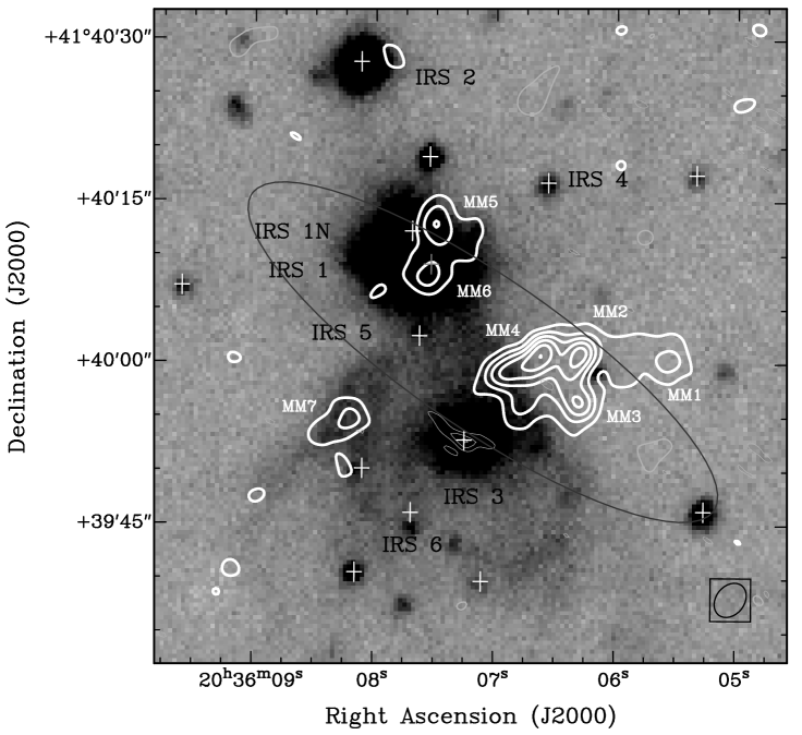
Figure 1: White (positive) and thick grey (negative) contours: SMA continuum emission at 1.3 mm towards the IRAS 20343+4129 region, obtained with natural weighting. Contours are $-3$, 3, 6, 9, 12, 15, and 18 times the rms noise, 2 mJy beam^-1. The synthesized beam, shown in the bottom right corner, is $3\aas@@fstack{\prime\prime}5\times 2\aas@@fstack{\prime\prime}6$, at $\mathrm{P.A.}=-38\aas@@fstack{\circ}0$. Thin grey contours: 3.6 cm emission obtained with the VLA (Sridharan et al. 2002). Contours are 3, 6, and 9 times the rms noise, 0.2 mJy beam^-1. Grey scale: H₂ emission (continuum plus line) at 2.12 $\mu$m from Kumar et al.  (2002). The crosses correspond to infrared sources from the 2MASS Point Source Catalog (PSC).

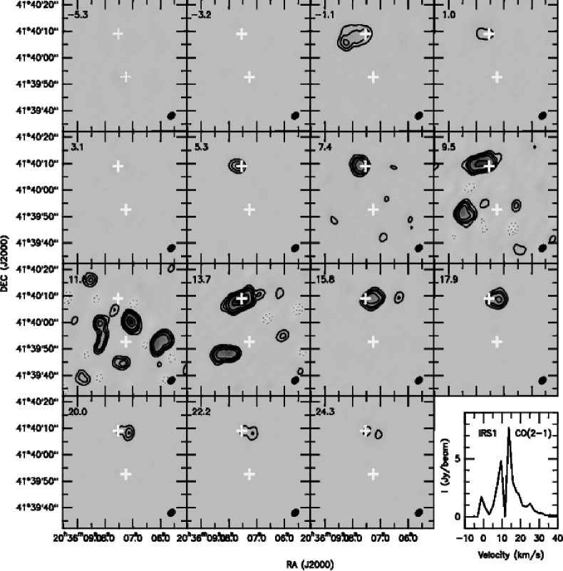
Figure 2: CO (2–1) channel maps of the IRAS 20343+4129 region, averaged over 2.11 km s^-1 wide velocity intervals. The central velocity of each channel is indicated in the upper left corner, and the systemic velocity is 11.5 km s^-1. The crosses indicate the position of IRS 1 (north) and IRS 3 (south). The synthesized beam, shown in the lower right corner, is $3\aas@@fstack{\prime\prime}5\times 2\aas@@fstack{\prime\prime}7$, at P.A.$=-37\aas@@fstack{\circ}8$. Contours are $-6$, $-3$, 3, 6, 9, 15, 30, and 40 times the rms noise, 0.4 Jy beam^-1. The lower right panel is the spectrum of the CO (2–1) emission toward the position of IRS 1. The conversion factor is 2.46 K (Jy/beam)^-1 (in the Rayleigh-Jeans assumption).

Figure 1 shows the continuum emission observed with the SMA at 1.3 mm. The emission is found basically toward three positions in the field: to the west of IRS 3 (where we found the strongest condensations, detected up to 18$\sigma$), to the east, and to the north of IRS 3 (where we found condensations up to 9$\sigma$). The condensations to the west and to the east of IRS 3 are coincident with the single-dish peaks of emission (Beuther et al. 2002a), and are not associated with any infrared source. The emission to the west of IRS 3 contains four condensations, MM1 to MM4, with a total flux density of 230 mJy (corrected for the primary beam response), while the emission to the east has one condensation, MM7, of only 28 mJy. This is different from the single-dish measurements, for which the eastern condensation is stronger than the western condensation by almost a factor of 2. We estimated that the SMA has picked up only 2% of the flux density of the single-dish eastern condensation (of $\sim\!30^{\prime\prime}$ in size), and 30% of the flux density of the single-dish western condensation (of $\sim\!20^{\prime\prime}$). Thus, the emission of the eastern condensation is essentially extended, and has been filtered out by the SMA, while the emission in the western condensation consists of different compact millimeter sources.

In Table 1 we list the position, peak intensity, flux density and mass for each millimeter continuum condensation detected above 5$\sigma$. In the derivation of the masses, we assumed that all of the continuum emission is dust emission which is optically thin, and adopted a gas-to-dust mass ratio of 100 and a dust mass opacity coefficient at 1.3 mm of 0.9 cm² g^-1 (agglomerated grains with thin ice mantles in protostellar cores of densities $\sim 10^{6}$ cm^-3; Ossenkopf & Henning 1994). There is a factor of 4 in the uncertainty of the masses due to uncertainties in the opacity law. As for the dust temperature, we found two estimates in the literature. From NH₃ observations toward this region, Miralles et al. (1994) derive a rotational temperature of $\sim\!20$ K, which can be considered a lower limit for the dust temperature, as gas from protostellar envelopes is mainly heated by collisions with warm dust grains (e. g., Ceccarelli et al. 1996). On the other hand, by fitting two greybodies to the spectral energy distribution of IRAS 20343+4129, Sridharan et al. (2002) obtain a dust temperature $T_{\mathrm{d}}$ for the cold component of 44 K. However, in this last estimate of $T_{\mathrm{d}}$, the flux densities were measured with single-dish telescopes with angular resolutions between 10^′′ and 100^′′, including the contribution from IRS 1, IRS 3 and other sources in the region. Thus, $T_{\mathrm{d}}=44$ K can be considered an upper limit. We adopt the intermediate value of $T_{\mathrm{d}}=30$ K.

The mass of MM7 is $\sim\!0.7$ $M_{\sun}$, and the total mass of MM1 to MM4 is $\sim\!6$ $M_{\sun}$. As a reference, the masses derived for the eastern and western single-dish condensations are 44 and 23 $M_{\sun}$, respectively (Beuther et al. 2002a, 2005; the authors adopt a dust temperature and an opacity law that yield masses very similar to those obtained using our assumptions). Thus, the millimeter compact sources detected with the SMA are embedded in a more massive gas halo. For MM6, the dust condensation associated with IRS 1, we obtained a mass of $\sim 0.8$ $M_{\sun}$. There is one condensation, MM5, $5^{\prime\prime}$ to the north of IRS 1 that is slightly offset ($\sim\!2^{\prime\prime}$) to the west of the infrared source IRS 1N (Fig. 1). Since the SMA and 2MASS positional uncertainties are $0\aas@@fstack{\prime\prime}5$ and $0\aas@@fstack{\prime\prime}6$ (Skrutskie et al. 2006), respectively, it is not clear from our data whether MM5 is associated with IRS 1N or is tracing a different source. Finally, we did not detect IRS 3 at 1.3 mm, setting an upper limit for its cirmcumstellar mass of $\sim\!0.2$ $M_{\sun}$. It is worth noting that IRS 3 is the only source associated with centimeter continnum emission in the field (see Fig. 1, and § 4.2).

3.2 CO (2–1)

Channel maps of the CO (2–1) emission are displayed in Fig. 2. CO (2–1) emission extends from $-2$ up to 33 km s^-1, with the systemic velocity being 11.5 km s^-1. The strongest CO (2–1) feature is associated with IRS 1, and spans several channels for blueshifted and redshifted velocities, as can be seen also in the spectrum of the CO (2–1) emission toward IRS 1 (Fig. 2).

The map of the low-velocity emission, integrated from 8.4 to 14.8 km s^-1, is shown in Fig. 3. From the figure, we can see clearly the association of CO (2–1) with IRS 1, as well as the presence of low-velocity components southwards of IRS 1 and surrounding IRS 3 that are associated with the large-scale CO(2–1) blueshifted lobe from Beuther et al. (2002b). It is worth noting that the two elongated structures on either side of IRS 3 seem to be associated with the fan-shaped structure found in H₂ by Kumar et al. (2002).

Regarding the high velocities, these are only present in the immediate surroundings of IRS 1. Figure 4a plots the integrated high-velocity emission toward IRS 1. Blue velocities have been integrated from $-6.4$ to 8.5 km s^-1, and red velocities from 14.7 to 32.8 km s^-1. The high-velocity CO (2–1) emission has a bipolar structure, with the center at the position of IRS 1, and is elongated in the east-west direction. Note that the red lobe splits up into two subcomponents.

A position-velocity (p-v) plot obtained toward IRS 1 in the east-west direction is shown in Fig. 4b. Up to $\pm 8^{\prime\prime}$ from the zero offset position, the emission shows a bipolar morphology, reaching high-velocities that are blueshifted for positive offsets (to the east), and redshifted for negative offsets (to the west). The distance from IRS 1 where we find high velocities allows us to constrain whether such velocities are due to gravitationally bound motions. We find weak high-velocity gas at $\sim\!12$ km s^-1 offset from the systemic velocity at position offsets up to $8^{\prime\prime}$, or 10000 AU. Such velocities at these distances would imply an extremely high central mass of $\sim\!1000$ $M_{\sun}$  for the motions to be gravitationally bound. Hence the bipolar structure seen in CO (2–1) toward IRS 1 is most likely tracing an outflow motion.

Additionally, we computed the p-v plot toward IRS 1 in the north-south direction (Fig. 4c). The only clear CO feature along the direction of the cut is the clump at the offset position zero, and does not seem related to any other CO feature to the south of IRS 1, although one would expect a north-south bipolar structure judging from the single-dish CO map from Beuther et al. (2002b). The CO emission at position zero arises from IRS 1, with the high-velocity component coming from outflow motions (see above). Note that observing outflow emission in both the east-west (Fig. 4b) and north-south (Fig. 4c) directions could be indicating that the IRS 1 outflow is a wide-angle outflow (this could be also an effect of not resolving the base of the outflow, but the high-velocity emission of Fig. 4c, specially in the blueshifted lobe, is partially resolved). Finally, the decrease in CO emission at around the systemic velocity near the zero offset position, also seen in the CO spectrum of Fig. 2, may be produced by a combination of the missing short spacings and opacity effects. Given that the brightness temperature at the line peak is around 20 K, similar to the kinetic temperature, the line is optically thick at systemic velocities. The CO emission at these velocities is probably self-absorbed by foreground quiescent material of the cloud in which the YSOs are embedded.

We calculated the energetics of the outflow associated with IRS 1 for each lobe separately, and listed the values in Table 2. The expression used for calculating the outflow CO column density $N(\mathrm{CO})$ from the transition $J\rightarrow J-1$ (derived from Eq. A1 of Scoville et al. 1986) is:

$$\left[\frac{N(\mathrm{CO})}{\mathrm{cm^{-2}}}\right]=4.33\times 10^{13}\frac{T_{\mathrm{ex}}}{J^{2}}\,\mathrm{exp}\left(\frac{2.77J(J+1)}{T_{\mathrm{ex}}}\right)\frac{\tau_{0}}{1-e^{-\tau_{0}}}\left[\frac{\int T_{\mathrm{B}}(v)dv}{\mathrm{K\leavevmode\nobreak\ km\leavevmode\nobreak\ s^{-1}}}\right],$$

where $T_{\mathrm{ex}}$ is the excitation temperature, $\tau_{0}$ is the optical depth, and $T_{\mathrm{B}}(v)$ is the brightness temperature profile.

For the mass derived from CO, we adopted a mean molecular weight per H₂ molecule of 2.8, and a CO abundance $X(\mathrm{CO})=10^{-4}$ (Scoville et al. 1986):

$$\left[\frac{M}{M_{\odot}}\right]=2.25\times 10^{-16}\left[\frac{A}{\mathrm{pc^{2}}}\right]\left[\frac{N(\mathrm{CO})}{\mathrm{cm^{-2}}}\right],$$

with $A$ being the area of the line emission.

We assumed optically thin emission in the line wing, and an excitation temperature of $\sim\!25$ K, estimated from the spectrum in Fig. 2. Due to the lack of observations of other CO transitions, we could not make a better estimate of $T_{\mathrm{ex}}$. However, this effect is small, as varying $T_{\mathrm{ex}}$ between 15 and 30 K yields to a variation in the outflow parameters of only $\sim\!7$%. For the red lobe we integrated from 15 to 33 km s^-1, and for the blue lobe from $-6$ to 8 km s^-1. The age or dynamical timescale $t_{\mathrm{dyn}}$ was derived by dividing the size of each lobe (from the first contour shown in Fig. 4a) by the maximum velocity reached in the outflow with respect to the systemic velocity (21.5 km s^-1  for the red lobe, and 17.5 km s^-1  for the blue lobe). We did not correct for the inclination angle, since this parameter is not well known. To apply this correction, the velocity must be divided by $\sin\ i$, and the linear size of the lobes must be divided by $\cos\ i$, with $i$ being the inclination angle with respect to the plane of the sky.

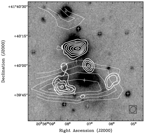
Figure 3: Thick contours: zero-order moment map for the low-velocity CO (2–1) emission. Velocities have been integrated from 8.4 to 14.8 km s^-1. Contours range from 8 to 56 Jy beam^-1 km s^-1, increasing in steps of 8 Jy beam^-1 km s^-1. Thin contours: zero-order moment of the blueshifted CO (2–1) emission observed in single-dish by Beuther et al. (2002b). Contours are 5.2, 6.3, 7.4, 8.5, and 9.6 $\rm Jy\leavevmode\nobreak\ beam^{-1}$ km s^-1. Grey scale: H₂ emission (continuum plus line) at 2.12 $\mu$m from Kumar et al.  (2002). Note that the SMA low-velocity structures on either side of IRS 3 are associated with H₂ extended emission. The crosses correspond to infrared sources from the 2MASS Point Source Catalog (PSC).

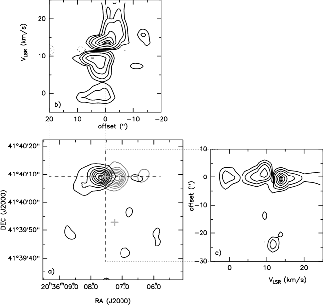
Figure 4: a) CO (2–1) high-velocity emission toward IRAS 20343+4129. Light grey contours, corresponding to the redshifted emission in a velocity range from 14.7 to 32.8 km s^-1, range from 2 to 38 Jy beam^-1 km s^-1, increasing in steps of 6 Jy beam^-1 km s^-1. Black contours, corresponding to the blueshifted emission in a velocity range from $-6.4$ to 8.5 km s^-1, are the same as light grey contours. Crosses mark the positions of IRS 1 (north) and IRS 3 (south). b) Position-velocity (p-v) plot along the east-west direction centered on IRS 1. Contours are $-5$, $-2$, 2, 5, 10, 20, 30, 40, and 45 times 0.4 Jy beam^-1. c) The same as in b) along the north-south direction.

Table 2: Physical parameters^a of the outflow driven by IRS1

	Age	$N_{12}$	Mass	$\dot{M}$	$P$	$\dot{P}$	$E_{\mathrm{kin}}$	$L_{\mathrm{mech}}$
Lobe	(yr)	(cm-2)	($M_{\sun}$)	($M_{\sun}$ yr-1)	($M_{\sun}$ km s-1)	($M_{\sun}$ km s-1 yr-1)	(erg)	($L_{\sun}$)
Red	3100	2.7$\times 10^{16}$	0.028	9.0$\times 10^{-6}$	0.50	1.6$\times 10^{-4}$	9.0$\times 10^{43}$	0.20
Blue	3800	2.6$\times 10^{16}$	0.027	7.2$\times 10^{-6}$	0.38	1.0$\times 10^{-4}$	5.3$\times 10^{43}$	0.09

• The parameters were obtained as follows. Age: $t_{\mathrm{dyn}}$ (see main text); mass-loss rate: $\dot{M}=M/t_{\mathrm{dyn}}$; momentum: $P=MV_{\mathrm{range}}$ ($V_{\mathrm{range}}$ is the range for which we integrated the emission for each lobe, see main text); momentum rate (or mechanical force): $\dot{P}=P/t_{\mathrm{dyn}}$; energy of the outflow: $E=1/2\leavevmode\nobreak\ M\leavevmode\nobreak\ V_{\mathrm{range}}^{2}$; mechanical luminosity: $L_{\mathrm{mech}}=E/t_{\mathrm{dyn}}$.

3.3 Infrared emission from 2MASS

We extracted a sample of infrared sources within the SMA primary beam toward IRAS 20343+4129 from the 2MASS Point Source Catalog (PSC, Skrutskie et al. 2006), with the aim of finding the possible infrared sources associated with the cloud of gas and dust studied in this work, and plotted their $(J-H)$, $(H-K)$ diagram (Fig. 5a). In the diagram, there are three sources with low values of the color indices, including IRS 3. These are unreddened (or only slightly reddened) stars. We measured the infrared excess as the difference between the $(H-K)$ color and the $(H-K)$ color correspoding to a reddened main-sequence star. There is a group of five sources, listed in Table 3, for which the infrared excess is larger than 1. We assume that such a large infrared excess (typically, infrared excesses for Class II sources are smaller than 0.4; Meyer et al. 1997) is indicative of the YSOs being associated with the IRAS 20343+4129 star-forming region. Out of these five sources, we detected dust continuum emission only toward IRS 1 and possibly IRS 1N.

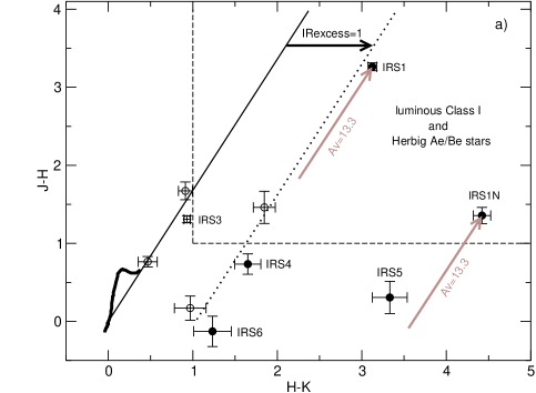
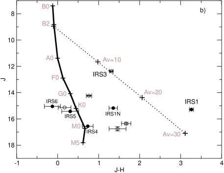
Figure 5: a) $(J-H)$, $(H-K)$ diagram of 2MASS sources within the SMA primary beam toward the IRAS 20343+4129 region. The infrared excess is measured with respect to the black thin solid line, which corresponds to the reddening line extending from the loci of main-sequence stars, marked with a black thick solid line (Allen 1976, and extinction law of Rieke & Lebofsky 1985). The dotted black line indicates the locus of sources with infrared excess equal to one. Note that IRS 3 has only a small infrared excess, while IRS 1 and IRS 1N are among the sources with highest infrared excess. Thin long-dashed lines mark the region in the diagram where most luminous Class I sources and Herbig Ae/Be stars are found (Lada & Adams 1992; Lee et al. 2005). b) $J$, $(J-H)$ diagram of the 2MASS sources in the IRAS 20343+4129 region. The solid black line indicates the locus of the main-sequence stars of different spectral types (Allen 1976). Note that when dereddening IRS 3 along the extinction vector (dotted line), it coincides with the position of B2 stars, for $A_{\mathrm{V}}=13.3$. In both panels, filled circles correspond to the sources with infrared excess larger than 1.

Table 3: 2MASS sources within the SMA primary beam with infrared excess $>1$

	Identification	Position					infrared
Source	2MASSJ+	$\alpha(\rm J2000)$	$\delta(\rm J2000)$	$J$	$H$	$K$a	excessb
IRS1	20360753+4140090	20:36:07.53	+41:40:09.1	15.28	12.02	8.90	1.17
IRS1N	20360769+4140121	20:36:07.69	+41:40:12.2	15.18	13.82	9.40	3.61
IRS3c	20360725+4139528	20:36:07.25	+41:39:52.8	12.37	11.06	10.13	0.15
IRS4	20360656+4140167	20:36:06.57	+41:40:16.7	16.56	15.82	14.17	1.21
IRS5	20360762+4140024	20:36:07.63	+41:40:02.5	15.43	15.12	11.79	3.15
IRS6	20360769+4139460	20:36:07.69	+41:39:46.1	15.05	15.17	13.94	1.31

• The filter is $K_{\mathrm{s}}$, but we write $K$ for simplicity.

• The infrared excess is measured as the difference between the measured $(H-K)$ color and the $(H-K)$ color correspoding to a reddened main-sequence star (Allen 1976, and extinction law of Rieke & Lebofsky 1985).

• Although IRS 3 does not have an infrared excess larger than 1, we include this source in the table due to its relevance in the paper.

In order to estimate the spectral type of the infrared sources, we plotted them in a $J$, $(J-H)$ diagram (Fig. 5b). In this diagram, if we deredden IRS 3 along the extinction vector, it falls at the position of B2 stars, consistent with the spectral type derived from its centimeter continuum emission (see § 4.2 and Miralles et al. 1994). Assuming that IRS 3 is a B2 main-sequence star, we derived the amount of visual extinction toward IRS 3, $A_{\mathrm{V}}=13.3$ mag. Regarding IRS 4, IRS 5 and IRS 6, they all have spectral types around K0 or later.

In the $(J-H)$, $(H-K)$ diagram of Fig. 5a, when dereddening IRS 1 and IRS 1N by $A_{\mathrm{V}}=13.3$ mag (the visual extinction toward IRS 3), we found that IRS 1 remains inside the loci of luminous Class I and Herbig Ae/Be stars (Lada & Adams 1992; Lee et al. 2005), while IRS 1N, after dereddening, has colors similar to YSOs of low luminosity.

4 Discussion

4.1 The young high-velocity bipolar outflow toward IRS 1

Small scale outflow found toward IRS 1:

The parameters of the IRS 1 outflow are similar to the mean values of low-mass outflows (Wu et al. 2004), and are about 2 orders of magnitude smaller than the parameters derived from surveys of high-mass outflows (Beuther et al. 2002b; Wu et al. 2005; Zhang et al. 2005; Xu et al. 2006). However, given that the surveys of high-mass molecular outflows are based on single-dish observations, picking up large-scale structure and considering thus larger areas of outflow emission, we compared the parameters of the IRS 1 outflow with other high-mass outflows observed with interferometers, listed in Table 4. From the table we found that the IRS 1 outflow is about 2–3 orders of magnitude less energetic than the outflows of high-mass protostars observed with high angular resolution. In some cases, the outflow parameters were corrected for opacity and inclination, but these effects may contribute only about 1 order of magnitude. From this comparison it seems that IRS 1 must be a low/intermediate-mass YSO.

Table 4: Physical parameters of the IRS1 outflow compared with other low, intermediate, and high-mass outflows observed with interferometers

	$L_{\mathrm{bol}}$	Age	Mass	$\dot{M}$	$P$	$\dot{P}$	$E_{\mathrm{kin}}$	$L_{\mathrm{mech}}$
Region	($L_{\sun}$)	(yr)	($M_{\sun}$)	($M_{\sun}$ yr-1)	($M_{\sun}$ km s-1)	($M_{\sun}$ km s-1 yr-1)	(erg)	($L_{\sun}$)	Ref.
HH 211	3.6	1400	0.0024	1.7$\times 10^{-6}$	0.040	2.8$\times 10^{-5}$	6.9$\times 10^{42}$	0.027	1
I21391	440	$-$	0.14	$-$	3.6	1.4$\times 10^{-3}$	1.2$\times 10^{45}$	$-$	2
I20343-IRS1	3200	3400	0.055	1.6$\times 10^{-5}$	0.88	2.6$\times 10^{-4}$	1.4$\times 10^{44}$	0.29	3
I20293-A	6300	4300	2.0	4.5$\times 10^{-4}$	90	2.1$\times 10^{-2}$	4.1$\times 10^{46}$	79	4
I18182	20000	$-$	7.3	$-$	71	$-$	8$\times 10^{45}$	$-$	5
ON2 N	$-$	37000	58	$-$	1060	2.8$\times 10^{-3}$	2.0$\times 10^{47}$	45	6

• 1: Palau et al. (2006); 2: Beltrán et al. (2002); 3: this work; 4: Beuther et al. (2004a); 5: Beuther et al. (2006); 6: Shepherd et al. (1997).

We additionally considered the centimeter continuum luminosity produced by shock ionization that should be observed for the IRS 1 outflow. From the correlation between the centimeter luminosity and the outflow momentum rate found by Anglada (1995) for a sample of low/intermediate-mass YSOs, the IRS 1 outflow can account for a centimeter luminosity of $\sim 0.6$ mJy kpc², assuming that all of the stellar wind is shocked. This centimeter luminositiy is undetectable with the sensitivity of the observations of Sridharan et al. (2002, shown in Fig. 1), which is on the order of $0.4$ mJy kpc². Then, the momentum rate derived for the outflow of IRS 1 is not able to produce a detectable amount of centimeter continuum emission, which is consistent with our observations.

Finally, the image of the H₂ line at 2.12 $\mu$m (1–0 S(1)) reveals strong emission very close to IRS 1 (Kumar et al. 2002), being elongated in the east-west direction, and thus coincident with the direction of the outflow of IRS 1. This would suggest that the H₂ emission at 2.12 $\mu$m close to IRS 1 arises from shocks in the outflow. However, Comerón et al. (2002) detected line emission at 2.225 $\mu$m, which could be due to the 1–0 S(0) line of H₂. This H₂ line at 2.225 $\mu$m has been found toward Class I and flat-spectrum sources (e. g., Doppmann et al. 2005), associated with outflows (Everett et al. 1995; Davis & Smith 1999; Caratti o Garatti et al. 2006), and with photon-dissociated regions (Ramsay et al. 1993; Luhman et al. 1998), but usually the H₂ line at 2.225 $\mu$m is much fainter than the H₂ line at 2.12 $\mu$m, while this is clearly not the case for IRS 1 (see Fig. 7 of Comerón et al. 2002). Ratios of different intensities of H₂ lines are used to discriminate between shock-excited H₂ emission and excitation by fluorescence. A detailed analysis of the ratios of high spectral resolution observations of different H₂ lines would allow us to study the mechanism of the H₂ excitation, but this is out of the scope of this paper.

Large-scale CO emission:

Single-dish observations of CO (2–1) toward IRAS 20343+4129 show a blue lobe centered around IRS 3, and a red single-peaked lobe around IRS 1 (Beuther et al. 2002b). H₂ emission in a fan-shaped structure is found to be associated with the blue CO large-scale lobe (see Fig. 3). This seems to suggest the existence of an outflow in the north-south direction. However, from the SMA data we found no evidence of such a north-south outflow (see Fig. 4a, c).

We compared the SMA CO (2–1) channel maps with the single-dish CO (2–1) channel maps of H. Beuther. The blue lobe observed with the single-dish data results from integrating only from 8 to 9 km s^-1, an interval very close to the systemic velocity. In the SMA channel maps from Fig. 2, we only detected emission at the position of the blue single-dish lobe for velocities between 8.4 and 14.8 km s^-1. Considering that the large-scale blue lobe arises from extended emission of $\sim\!25^{\prime\prime}$ in size, we found that this emission could not have been detected by the SMA. Given the shortest baseline of an interferometer, and the size of the observed emission, one can estimate the fraction of correlated flux detected by the interferometer. For a source of $25^{\prime\prime}$, this corresponds to a 0.2% for our SMA configuration (with a shortest baseline of 11 k$\lambda$). Thus, out of the total CO (2–1) flux observed in single-dish for the blue lobe, 1310 Jy km s^-1, the SMA could pick up only 2.6 Jy km s^-1, which should be detected at a few times the rms of the SMA channel maps, as is the case (see channel at 9.5 km s^-1 of Fig. 2). We concluded that almost all of the large-scale blueshifted lobe seen in single-dish has been resolved out by the SMA. Note that in the single-dish images of Beuther et al. (2002b) there is a blue contour at the position of IRS 1, suggesting that if blueshifted emission had been integrated for velocities $<8$ km s^-1, the blue lobe of the IRS 1 outflow detected with the SMA would appear in the single-dish observations as well.

Regarding the single-dish red lobe, this was obtained integrating from 13 to 15 km s^-1 (Beuther et al. 2002b). We estimated the contribution of the SMA redshifted emission to the single-dish redshifted emission. The SMA integrated intensity of the red lobe for the same range of velocities as Beuther et al. (2002b) is 160 Jy km s^-1, obtained from the spectrum toward IRS 1, and assuming a size of the lobe of $\sim 10^{\prime\prime}$. Beuther et al. (2002b) obtain a flux density of 1300 Jy km s^-1, implying that the SMA redshifted emission can account for about 12% of the redshifted emission detected with the single-dish data, a contribution about 2 orders of magnitude higher than that for the blueshifted large-scale lobe. This suggests that the blue and red lobes seen in the single-dish data, come from material at different spatial scales.

4.2 Is IRS 3 driving a cavity around it?

As seen above, the CO (2–1) emission from the single-dish data (Beuther et al. 2002b) shows a slightly blueshifted large-scale lobe that corresponds well with the fan-shaped structure seen in H₂ emission around IRS 3 (see Fig. 3). In addition, from the SMA data of this work, we found low-velocity CO elongated structures on either side of IRS 3, as well as dust condensations also on either side of IRS 3. All these observational features seem to suggest that IRS 3 is interacting with the surrounding medium and producing a shell of circumstellar gas expanding away from IRS 3. We search for any kinematical evidence of such an expanding cavity in the low-velocity CO emission, but the strong missing flux, and the presence of at least one bipolar outflow and other YSOs surrounding IRS 3, make this search difficult. However, a preliminary study of the NH₃ emission in the region revealed dense gas surrounding IRS 3 whose kinematics were consistent with an expanding shell with IRS 3 in its center (Palau et al., in prep.). In the following, we consider whether IRS 3 is able to drive such a cavity.

Given that the centimeter continuum emission associated with IRS 3 (of 1.8 mJy, Sridharan et al. 2002) is consistent with an ionizing B2 star (Panagia 1973), and that the luminosity-to-mass ratio of typical B2 stars is high enough to allow the star to push away the surrounding material by radiation pressure (given typical dust opacities of molecular clouds, Calvet et al. 1991; Anglada et al. 1995), the first interpretation to explore is that the cavity is driven by the radiation pressure from IRS 3. This leads to a scenario in which IRS 1 is a low/intermediate-mass YSO accounting for a small fraction of the total bolometric luminosity of IRAS, while IRS 3 is a high-mass star accounting for most of the bolometric luminosity. However, the cavity could also be driven by a stellar wind from IRS 3. We studied the scenario of a wind-driven cavity by following the model of Anglada et al. (1995). In this model, the centimeter continuum emission is assumed to trace an ionized stellar wind. We adopted a spectral index for the wind of 0.6, and estimated a mass loss rate of the ionized material following Beltrán et al. (2001). By noting from the observations the radius of the cavity ($\sim\!10^{\prime\prime}$), the velocity of its walls ($\sim\!2$ km s^-1), and the external pressure of the ambient cloud ($\sim\!3.3$ km s^-1, from the line width of the CO (2–1) line in the walls of the cavity), we obtained a maximum radius, density, and dynamical timescale of the cavity of 12^′′, 2300 cm^-3, and 11000 yr, respectively, which are reasonable values for the region. This leads to a scenario in which IRS 3 is not necessarily the most massive source of the region, and then IRS 1 could account for most of the IRAS luminosity.

Table 5: Summary of the centimeter observations carried out toward IRAS 20343+4129

$\lambda$	$S_{\mathrm{\nu}}$	Observing	$\theta_{\mathrm{FWHM}}$
(cm)	(mJy)	year	(′′)	Refs.
6	$1.1\pm 0.2$	1989	$5^{\prime\prime}$	Miralles et al. (1994)
3.6	$1.3\pm 0.3$	1994	$8^{\prime\prime}$	Carral et al. (1999)
	$1.8\pm 0.1$	1998	$1^{\prime\prime}$	Sridharan et al. (2002)
2	$<1.0$a	1989	$5^{\prime\prime}$	Miralles et al. (1994)
0.7	$<9$a	2003	$1\aas@@fstack{\prime\prime}5$	Menten et al., in prep.

• Upper limits at the 3$\sigma$ level.

Thus, in the interpretation of the centimeter continuum emission as either an UCH ii region, or an ionized stellar wind, IRS 3 can create a cavity of swept up material around it. In order to distinguish between these two scenarios, it would be very useful to consider the spectral energy distribution in the centimeter range for IRS 3. In addition to the 3.6 cm measurement from Sridharan et al. (2002), shown in this work, there are other observations at 6, 3.6, and 2 cm, listed in Table 5. The only simultaneous measurements are those at 6 and 2 cm, which result in a spectral index $\leq-0.1$, consistent with an optically thin UCH ii region. However, the other observations at 3.6 cm are not consistent with this flat spectral index. With the measurements at 3.6 and 6 cm, the spectral index ranges from 0.3 to 0.9 (depending on the epoch of the observations at 3.6 cm). This spectral index is consistent with emission from an ionized wind (e. g., Panagia & Felli 1975). Thus, from the current data it is not clear whether the source is variable with time, and what is the value of the spectral index of the centimeter source associated with IRS 3. New observations at 6, 3.6, 2, and 1.3 cm toward IRS 3 would give insight into which mechanism, a stellar wind or radiation pressure, is driving the cavity.

4.3 On the nature of IRS 1

From an analysis of $JHK$ color-magnitude diagrams including the high-mass stars of the Cygnus OB2 association, Comerón et al. (2002) propose that IRS 1 may be one of the most luminous and embedded objects in the entire association. In the $K$, $(H-K)$ diagram, IRS 1 is the reddest object of the association, and dereddening along the extinction vector yields a very bright $K$ magnitude compared with the other massive stars. However, this plot sets an upper limit to the intrinsic brightness because in the $K$ band there may be some contribution from circumstellar material. For this reason, Comerón et al. (2002) use the $H$, $(J-H)$ diagram, which is not seriously affected by circumstellar emission, and find again that IRS 1 is among the brightest. Since the color-magnitude diagrams were made by using the Second Incremental Release of the 2MASS Point Source Catalog (PSC), and this release is by now obsolete, we redid the diagrams with magnitudes from the current release of 2MASS PSC, and found the same values except for the $J$ magnitude, yielding $(J-H)=3.26$ instead of 4.23 used by Comerón et al. (2002). Thus, dereddening along the extinction vector in the $H$, $(J-H)$ diagram does not set IRS 1 among the brightest members of the association, but yields that IRS 1 must be still intrinsically brighter than stars with spectral type B0, for which typical luminosities are around 25000 $L_{\sun}$ (Panagia 1973), at least one order of magnitude higher than the bolometric luminosity of IRAS 20343+4129.

If IRS 1 were a high-mass ZAMS star, one would expect to detect centimeter continuum emission from ionized gas, and to detect the star at optical wavelengths. However, no centimeter continuum emission was detected above the 3$\sigma$ level of 0.6 m$\rm Jy\leavevmode\nobreak\ beam^{-1}$, and IRS 1 does not appear in the POSSII plates. If IRS 1 were a high-mass protostar, deeply embedded and still accreting most of its mass, one would expect to observe a massive envelope, with a mass of the order of the accreted mass, surrounding the protostar. But we did not detect a massive envelope toward IRS 1 from the millimeter continuum emission (the circumstellar mass was $\sim\!0.8$ $M_{\sun}$, § 3.1), and the outflow parameters were comparable to those of low/intermediate-mass protostars (§ 4.1). Thus, a high-mass nature for IRS 1 is not consistent with our observations. All this suggests that IRS 1 cannot be considered a reddened stellar photosphere but a YSO with a cold envelope, and that the estimation of its brightness from the magnitude-color diagrams gives only an upper limit. Note however that the $JHK$ magnitudes of IRS 1 cannot be accounted for by a low-mass YSO at the distance of the region.

At this point we consider whether the continuum emission is really tracing all the dust surrounding IRS 1. We considered four different possibilities. First, the SMA could be filtering out large-scale emission; we considered this option and we ruled it out because the largest angular scale (FWHM) to which the SMA is sensitive is $\sim\!8^{\prime\prime}$, larger than $\sim\!4^{\prime\prime}$, the observed size of the millimeter source associated with IRS 1 (MM6). In addition, the CO emission observed with the SMA toward IRS 1 shows that the SMA is really sensitive to scales larger than the size of the dust condensation associated with IRS 1, and that the dust emission is significantly more compact than the CO emission. Second, the dust could be optically thick; however, this possibility yields an unrealistically low value for the dust temperature, given the flux density at 1.3 mm and the deconvolved size for MM6 of $3^{\prime\prime}$. Third, the dust could be sublimated; since dust sublimates at $\sim\!1500$ K (Whitney et al. 2004), a considerable amount of gas at such a high temperature should be detected at optical wavelengths. Fourth, CO emission has been detected with no continuum emission for a few YSOs; however, these objects are evolved (Class II/III) low-mass systems (e. g., Andrews & Williams 2005; Takeuchi & Lin 2005). Thus, none of these possibilities is convincing for the case of IRS 1, hinting that the mass traced by the millimeter continuum emission is most likely all the circumstellar mass associated with IRS 1.

Therefore, the current data suggest that IRS 1 is a low/intermediate-mass YSO. In order to further constrain the mass and the evolutionary stage of IRS 1, we plotted the spectral energy distribution (SED) compiled from 2MASS (corrected for interstellar extinction, see § 3.3), MSX, IRAS, observations in the submillimeter range carried out with SCUBA on the JCMT (Williams et al. 2004), and the SMA (this work). As the IRAS flux densities may have contribution from both IRS 1 and IRS 3, they are only upper limits. The fluxes measured by SCUBA are also upper limits because the single dish is picking up large-scale emission, partially arising from IRS 3 and from the dust condensations on either side of IRS 3. The angular resolution of the MSX images allowed us to estimate the flux density from IRS 1 by integrating the mid-infrared emission in an aperture of $\sim\,15^{\prime\prime}$ of diameter around IRS 1.

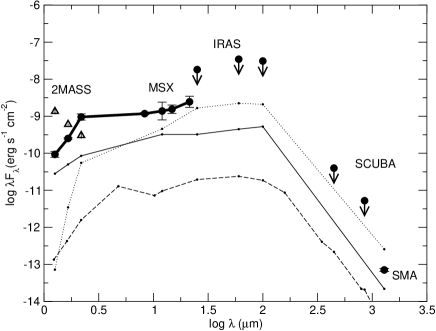
Figure 6: Spectral Energy Distribution (SED) for IRS 1. Black dots correspond to IRS 1, and thin curves are SEDs from the literature for Class I sources of 960 $L_{\sun}$ (dotted, VMR-D-IRS 13: Massi et al. 1999), 250 $L_{\sun}$ (solid, VMR-D-IRS 14: Massi et al. 1999), and 4 $L_{\sun}$ (dashed, IRAS 04016+2610: Eisner et al. 2005), which have been scaled to the distance of IRAS 20343+4129. IRAS and SCUBA fluxes are upper limits because it is not possible to disentangle the contribution of IRS 1 from the surrounding sources. For comparison, open triangles correspond to IRS 3 2MASS fluxes. 2MASS fluxes have been corrected for interstellar extinction (see § 3.3).

The resulting SED (Fig. 6) shows a steep profile for the 2MASS wavelengths, suggesting that any contribution from a hot photosphere is negligible. Rather, the peak of the SED lying between 10 and 100 $\mu$m indicates that most likely a cold envelope dominates the SED, with d(log$\lambda F_{\lambda}$)/d(log$\lambda$)$>0$ between 2 and 100 $\mu$m, consistent with the classification of IRS 1 as a Class I source (e. g., Hartmann 1998). Note that if IRS 1 were a Class 0 source, the SED should not show significant emission in the near infrared (André et al. 1993; Lada 1999). We compared the IRS 1 SED with SEDs of Class I sources of bolometric luminosities between 4 and 960 $L_{\sun}$ from the literature, scaled to the distance of IRAS 20343+4129. From this comparison, we found that IRS 1 is likely not a low-mass source, but rather its SED resembles that of intermediate-mass sources with bolometric luminosities around 1000 $L_{\sun}$  (the exact value of the luminosity of IRS 1 cannot be determined because the IRAS flux densities are only upper limits, and could be the main contribution to the bolometric luminosity). From the evolutionary tracks of Palla & Stahler (1993) for intermediate-mass stars, and assuming that IRS 1 is already in the birthline, one would expect a stellar mass for IRS 1 of around 5 $M_{\sun}$. This is a factor of 6 higher than the circumstellar mass derived from the SMA data, $\sim\!0.8$ $M_{\sun}$ (§ 3.1). In the low-mass regime, Class 0 sources are expected to have circumstellar/envelope masses similar to the stellar masses, and thus one could argue that $0.8$ $M_{\sun}$ is too low for an intermediate-mass YSO of 1000 $L_{\sun}$. However, one expects that in the Class I stage, the ratio of the circumstellar-to-stellar mass progressively decreases. Taking into account that intermediate-mass sources evolve faster to the main-sequence than the low-mass sources, it may be reasonable to have a circumstellar mass lower than its stellar mass. In addition, there are some cases in which the mass of the dust/gas condensation associated with intermediate-mass YSOs is significantly lower (at least by 1 order of magnitude) than the estimated stellar mass (Beuther et al. 2004b; Martín-Pintado et al. 2005; Zapata et al. 2006). Thus, a circumstellar mass of $\sim\!0.8$ $M_{\sun}$ for IRS 1 seems to be compatible with its classification as a Class I source of around 1000 $L_{\sun}$.

4.4 Sources in different evolutionary stages: millimeter vs near-infrared emission

In order to gain insight into the star formation process in the region, we tentatively classified the different sources identified in this work in three different evolutionary stages, depending on their millimeter and infrared emission.

Sources at the end of the accretion phase:

We classified in this evolutionary stage IRS 3 to IRS 6 (Table 3), the sources detected only in the infrared. From the centimeter and infrared emission, IRS 3 seems to be a B2 star. As for IRS 4 to IRS 6, they all have spectral types around K0 or later (as shown in Fig. 5b), and thus are low-mass YSOs. Since we did not detect emission toward these sources at 1.3 mm, we estimated an upper limit for their associated mass of $\sim\!0.2$ $M_{\sun}$  (with the same assumptions as § 3.1). These YSOs are possibly Class II/III sources.

Sources in the main accretion phase:

We included in this group the sources showing both infrared and millimeter emission, as is the case of IRS 1. In § 3.3 and 4.3 we concluded that IRS 1 seems to be an intermediate-mass Class I source. Another source that could be in the main accretion phase is IRS 1N, if we assume that it is associated with MM5 (see § 3.1). For this source we estimated a spectral type A0 or later, from the magnitude-color diagram of Fig. 5b, and an associated mass of $\sim\!0.9$ $M_{\sun}$, from the SMA data. Thus, if IRS 1N is an embedded YSO, it is a low-mass object. However, IRS 1N is the source with the highest $H-K$ color in the region (see Fig. 5a), and a possibility for such a high $H-K$ color is that the $K$-band is contaminated by the H₂ line at 2.12 $\mu$m, as the continuum-subtracted H₂ images from Kumar et al. (2002) suggest. Thus, it remains unclear from the available data whether IRS 1N is a low-mass embedded YSO, or an infrared source whose emission mainly arises in the interaction of an outflow (either the IRS 1 outflow, or an outflow from IRS 1N/MM5 itself) with the surrounding medium.

Starless core candidates:

The sources MM1 to MM4 and MM7 (Table 1) have been detected only in the millimeter, and lie in a region completely dark in the near infrared (Fig. 1). The masses of these dust condensations are 0.7–1.2 $M_{\sun}$, and thus they are low-mass condensations. Sources bright only in the millimeter could also be tracing Class 0 protostars being at the beginning/main accretion phase. However, given that we did not find any sign of star formation such as outflow emission, we suggest that some, if not all, of these sources could be starless core candidates.

Therefore, the IRAS 20343+4129 region harbors sources that seem to be in different evolutionary stages, and with stellar masses ranging from $<0.2$ to 8–10 $M_{\sun}$. The intermediate/high-mass sources of the region, IRS 1 and IRS 3, are in different evolutionary stages. IRS 3 is visible at optical wavelengths, does not show infrared excess, and has no CO (2–1) nor dust emission associated, suggesting that it has already finished the main accretion phase. On the contrary, IRS 1 is not detected in the optical, has strong infrared excess and dust emission associated, and is the driving source of a bipolar outflow, which indicates that IRS 1 is still accreting a significant amount of mass, with IRS 1 therefore younger than IRS 3. However, even with different evolutionary stages, IRS 1 and IRS 3 could have formed simultaneously, since the uncertainty in their masses is important, and the contraction time to the main-sequence (since the formation of a first hydrostatic core until the hydrogen burning stage), which deacreases with the mass of the YSO, in the intermediate/high-mass regime gets comparable or shorter than the free-fall timescale, and thus an intermediate-mass Class I YSO may have formed simultaneously with a high-mass object already in the main-sequence phase. For example, using the computations of Bernasconi & Maeder (1996), and assuming that IRS 3 is around 9 $M_{\sun}$  and IRS 1 is around  5 $M_{\sun}$, IRS 3 has a contraction time of $\sim\!0.3$ Myr, and IRS 1 of $\sim\!1$ Myr. This is different from the low-mass regime, where YSOs evolve to the main-sequence in a timescale $>10$ Myr (e. g., Hayashi 1961; Iben 1965), which is always much larger than the free-fall timescale ($\sim 0.5$ Myr). Thus, a low-mass YSO in the pre-main-sequence phase (Class II/III) and a low-mass YSO in the main accretion phase (Class 0/I) cannot have formed simultaneously. As seen in this section, we find low-mass YSOs in the very first phases of formation, and others that seem to be Class II/III candidates, and thus they cannot be coeval. Therefore, the star formation in IRAS 20343+4129 seems to be a continuous process. It is worth noting that the intermediate/high-mass star IRS 3 is in an evolutionary stage equal or more evolved than the low-mass sources. This is in contrast to previous claims that intermediate/high-mass stars in clusters appear less evolved than the low-mass stars in the cluster (Massi et al. 2000; Kumar et al. 2006).

Finally, the spatial distribution of the sources found in IRAS 20343+4129 shows that star formation in this region is localized, that is, to the north and south of IRS 3 there are YSOs that are already bright in the infrared, while to the east and to the west there are millimeter sources that seem to be starless cores. Since IRS 3 and IRS 1 could be coeval, we suggest that these two sources are reflecting the initial conditions of high density in the parental cloud. As for the low-mass dust condensations on either side of IRS 3, we propose that they may be compressed by the expanding cavity driven by IRS 3, and thus could eventually form a new generation of stars.

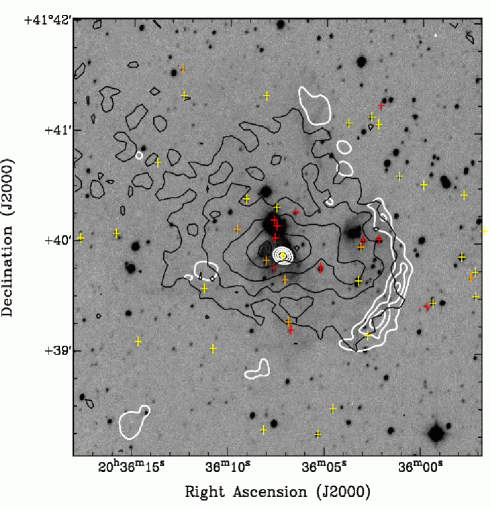
Figure 7: Grey scale: H₂ emission (continuum plus line) at 2.12 $\mu$m in the IRAS 20343+4129 region (Kumar et al. 2002). White contours correspond to the 3.6 cm emission from Carral et al. (1999), and are 0.66, 0.99, 1.14, 1.33, 1.52, and 1.71 m$\rm Jy\leavevmode\nobreak\ beam^{-1}$. Black contours are the 1.2 mm continuum emission observed in single dish by Beuther et al. (2002a), and trace the dust cloud where IRS 1 and IRS 3 are forming. Contours are: 25, 50, 100, 200, and 300 m$\rm Jy\leavevmode\nobreak\ beam^{-1}$. Note that the centimeter emission traces the ionized southwestern border of the cloud, as well as IRS 3 in the center of the cloud. Crosses indicate the spatial distribution of the 2MASS sources in the region with infrared excess larger than zero: (0–0.4) for the yellow color (Class II sources); (0.4–1) for the orange color (Class I), and $>1$ for the red color, following Matsuyanagi et al. (2006). Note that most of the 2MASS sources with infrared excess $>1$ lie in the center of the cloud, near IRS 3 and IRS 1.

4.5 IRAS 20343+4129 within Cygnus OB2

The H₂ emission at 2.12 $\mu$m shows a cometary arch about $1^{\prime}$ to the southwest of IRS 3, which is also detected in centimeter emission (see Fig. 7; Kumar et al. 2002; Carral et al. 1999). This cometary arch follows the border of a dust cloud traced by 1.2 mm emission observed in single-dish by Beuther et al. (2002a), and could be produced by the ionization front from a nearby OB star. In fact, the arch is facing the center of the Cygnus OB2 association. This would be similar to the bright-rimmed clouds facing HII regions, such as IC 1396N (Sugitani et al. 1991; Beltrán et al. 2002), which is ionized by an O6.5 star at 13 pc of distance (Schwartz et al. 1991). We plotted the OB stars of the association (Reed 2003), and found that there are five O6–O9 stars about 25^′ (9 pc at the adopted distance for IRAS 20343+4129) to the south-west of the arch. Given the flux density of the centimeter continuum emission tracing the cometary arch, one can estimate the required flux of ionizing photons per unit area that must reach the cloud to produce the observed centimeter emission (Lefloch et al. 1997). In our case, the flux density of the arch at 3.6 cm is around 5 mJy, and this requires a flux of ionizing photons per area unit of $4\times 10^{9}$ s^-1 cm^-2. The flux of ionizing photons for an O6 star is tipically $1.20\times 10^{49}$ s^-1 (Panagia 1973), and assuming a distance to the arch of 9 pc, the flux of ionizing photons per area unit reaching the cloud is $1.2\times 10^{9}$ s^-1 cm^-2, close to the value required to account for the flux of the centimeter emission in the arch. Thus, the O6 star $25^{\prime}$ to the southwest of the arch, BD+41 3807, is probably the star ionizing the border of the IRAS 20343+4129 cloud. Finally, we calculated the infrared excess (as described in § 3.3) of the 2MASS sources within a diameter of 4^′ centered on IRS 3 (thus including a region outside the rim), and plotted the sources with positive infrared excess in Fig. 7. In the figure, crosses with redder colors correspond to sources with larger infrared excess (and thus presumably younger). As seen from the figure, most of the sources with strongest infrared excess within the field are found inside the cloud, thus constituting a region of recent star formation as compared to its surroundings. In addition, the millimeter sources detected in this work could be sites of future star formation, and thus IRAS 20343+4129 is a region actively forming stars within the Cygnus OB2 association.

5 Conclusions

We observed the dust continuum emission at 1.3 mm with the SMA as well as the CO (2–1) emission toward the massive star-forming region IRAS 20343+4129, in order to study the properties of the different protostars in the region and their interactions with the surrounding medium. Two bright infrared sources, IRS 1 in the north and IRS 3 in the south, lie inside the SMA primary beam, and IRS 3 is associated with centimeter continuum emission. Our main conclusions can be summarized as follows:

1. The dust continuum emission reveals three main condensations, to the north (associated with IRS 1), to the east and to the west of IRS 3, with the western condensation being the brightest one and consisting of different subcondensations, of $\sim\!1$ $M_{\sun}$ each. Toward the eastern condensation, of $\sim\!0.7$ $M_{\sun}$, the SMA has filtered out most of the emission. The estimated mass of the condensation associated with IRS 1 is $\sim\!0.8$ $M_{\sun}$.

2. We discovered a bipolar high-velocity CO outflow, elongated in the east-west direction, and identified IRS 1 as its driving source. The millimeter continuum and CO emissions indicate that IRS 1 is not a high-mass YSO, and the SED agrees with IRS 1 being an intermediate-mass Class I source.

3. The low-velocity CO emission shows, in addition to emission toward IRS 1, two elongated structures on either side of IRS 3, coincident with extended H₂ emission at 2.12 $\mu$m. The emission from the blueshifted lobe of the large-scale CO outflow seen in single-dish by Beuther et al. (2002b) has been filtered out by the SMA, and the lobe does not have compact emission. A scenario in which the blue large-scale CO lobe traces a cavity blown up by IRS 3, and where the dust condensations on either side of IRS 3 are the result of the accumulation of mass in the walls of the expanding cavity, is consistent with the observations. In this scenario, the elongated low-velocity CO emission and the H₂ extended emission trace the walls of the cavity. The expanding cavity could be either driven by a stellar wind from IRS 3, or driven by radiation if we assume that IRS 3 is a B2 star.

4. We found objects with very different properties and evolutionary stages that have been born in the same parental cloud. In addition, these objects are not randomly distributed in the cloud, but their distribution seems to be determined, at least partially, by the accumulation of mass at the walls of an expanding cavity driven by IRS 3.

- (1) Allen, C. W. 1976, Astrophysical Quantities, 3rd edn., London: Athlone Press
- (2) André, P., Ward-Thompson, D., & Barsony, M. 1993, ApJ, 406, 122
- (3) Andrews, S.M., & Williams, J.P. 2005, ApJ, 619, L175
- (4) Anglada, G. 1995, RMxAA, 1, 67
- (5) Anglada, G., Estalella, R., Mauersberger, R., et al. 1995, ApJ, 443, 682
- (6) Beltrán, M. T., Estalella, R., Anglada, G., Rodríguez, L. F., & Torrelles, J. M. 2001, AJ, 121, 1556
- (7) Beltrán, M. T., Girart, J. M., Estalella, R., Ho, P. T. P., & Palau, A. 2002, ApJ, 573, 246
- (8) Bernasconi, P. A., & Maeder, A. 1996, A&A, 307, 829
- (9) Beuther, H., Schilke, P., & Gueth, F. 2004a, ApJ, 608, 330
- (10) Beuther, H., Schilke, P., Menten, K. M., et al. 2002a, ApJ, 566, 945
- (11) Beuther, H., Schilke, P., Menten, K. M., et al. 2005, ApJ, 633, 535
- (12) Beuther, H., Schilke, P., Sridharan, T. K., et al. 2002b, A&A, 383, 892
- (13) Beuther, H., Zhang, Q., Greenhill, L. J., et al. 2004b, ApJ, 616, L31
- (14) Beuther, H., Zhang, Q., Sridharan, T. K., Lee, C.-F., & Zapata, L. A. 2006, A&A, 454, 221
- (15) Bontemps, S., André, P., Terebey, S., & Cabrit, S. 1996, A&A, 311, 858
- (16) Calvet, N., Patiño, A., Magris, G., & D’Alessio, P. 1991, ApJ, 380, 617
- (17) Caratti o Garatti, A., Giannini, T., Nisini, B. & Lorenzetti, D. 2006, A&A, 449, 1077
- (18) Carral, P., Kurtz, S., Rodríguez, L. F., et al. 1999, RMxA&A, 35, 97
- (19) Ceccarelli, C., Hollenbach, D. J., & Tielens, A. G. G. 1996, ApJ, 471, 400
- (20) Comerón, F., Pasquali, A., Rodighiero, G., et al. 2002, A&A, 389, 874
- (21) Davis, C. J., Smith, M. D., Eislöffel, J., & Davies, J. K. 1999, MNRAS, 308, 539
- (22) Doppmann, G. W., Greene, T. P., Covey, K. R., & Lada, C. J. 2005, ApJ, 130, 1145
- (23) Eisner, J. A., Hillenbrand, L. A., & Carpenter, J. M. 2005, ApJ, 635, 396
- (24) Everett, M. E., Depoy, D. L., Pogge, R. W. 1995, AJ, 110, 1295
- (25) Fontani, F., Caselli, P., Crapsi, A., et al. 2006, A&A, 460, 709
- (26) Fuller, G. A., Williams, S. J., & Sridharan, T. K. 2005, A&A, 442, 949
- (27) Hartmann, L. 1998, Accretion Processes in Star Formation, eds. A. King, D. Lin, S. Maran, J. Pringle, & M. Ward, Cambridge: Cambridge University Press, p. 8
- (28) Hayashi, C. 1961, PASJ, 13, 450
- (29) Ho, P.T.P., Moran, J.M., & Lo, K.Y. 2004, ApJ, 616, L1
- (30) Iben, I., Jr. 1965, ApJ, 141, 993
- (31) Kumar, M. S. N., Bachiller, R., & Davis, C.J. 2002, ApJ, 576, 313
- (32) Kumar, M. S. N., Keto, E., & Clerkin, E. 2006, A&A, 449, 1033
- (33) Lada, C. J. 1999, in The Origin of Stars and Planetary Systems, eds. C. J. Lada, and N. D. Kylafis, Kluwer Acad. Publ., p. 143
- (34) Lada, C. J., & Adams, F. C. 1992, ApJ, 393, 278
- (35) Le Duigou, J.-M., & Knödlseder, J. 2002, A&A, 392, 869
- (36) Lee, H.-T., Chen, W. P., Zhang, Z.-W., & Hu, J.-Y. 2005, ApJ, 624, 808
- (37) Lefloch, B., Lazareff, B., & Castets, A. 1997, A&A, 324, 249
- (38) Luhman, K. L., Engelbracht, C. W., & Luhman, M. L. 1998, ApJ, 499, 799
- (39) Martín-Pintado, J., Jiménez-Serra, I., Rodríguez-Franco, A., Martín, S., & Thum, C. 2005, ApJ, 628, L61
- (40) Massi, F., Giannini, T., Lorenzetti, D., et al. 1999, A&AS, 136, 471
- (41) Massi, F., Lorenzetti, D., Giannini, T., & Vitali, F. 2000, A&A, 353, 598
- (42) Matsuyanagi, I., Itoh, Y., Sugitani, K., Oasa, Y., Mukai, T., et al. 2006, PASJ, 58, L29
- (43) Meyer, M. R., Calvet, N., & Hillenbrand, L. A. 1997, AJ, 114, 288
- (44) Miralles, M. P., Rodríguez, L. F., & Scalise, E. 1994, ApJSS, 92, 173
- (45) Ossenkopf, V., & Henning, Th. 1994, A&A, 291, 943
- (46) Palau, A., Ho, P. T. P., Zhang, Q., et al. 2006, ApJ, 636, L137
- (47) Palla, F., & Stahler, S.W. 1993, ApJ, 418, 414
- (48) Panagia, N. 1973, AJ, 78, 929
- (49) Panagia, N., & Felli, M. 1975, A&A, 39, 1
- (50) Ramsay, S. K., Chrysostomou, A., Geballe, T. R., Brand, P. W. J. L., & Mountain, M. 1993, MNRAS, 263, 695
- (51) Reed, B. C. 2003, AJ, 125, 2531
- (52) Richards, P. J., Little, L. T., Toriseva, M., & Heaton, B.D. 1987, MNRAS, 228, 43
- (53) Rieke, G. H., & Lebofsky, M. J. 1985, ApJ, 288, 618
- (54) Sault, R. J., Teuben, P. J., & Wright, M. C. H. 1995, in ASP Conf. Ser. 77, Astronomical Data Analysis Software and Systems IV, ed. R. A. Shaw, H. E. Payne, & J. J. E. Hayes, San Francisco: ASP, p. 433
- (55) Scoville, N. Z., Sargent, A. I., Sanders, D. B., et al. 1986, ApJ, 303, 416
- (56) Shepherd, D. S., Churchwell, E., & Wilner, D. J. 1997, ApJ, 482, 355
- (57) Skrutskie, M. F., Cutri, R. M., Stiening, R., et al. 2006, AJ, 131, 1163
- (58) Sridharan, T. K., Beuther, H., Schilke, P., Menten, K. M., & Wyrowski, F. 2002, ApJ, 566, 931
- (59) Sugitani, K., Fukui, Y., & Ogura, K. 1991, ApJS, 77, 59
- (60) Schwartz, R. D., Gyulbudaghian, A. L., & Wilking, B. 1991, ApJ, 370, 263
- (61) Takeuchi, T., & Lin, D. N. C. 2005, ApJ, 627, 286
- (62) Whitney, B. A., Indebetouw, R., Bjorkman, J. E., & Wood, K. 2004, ApJ, 617, 1177
- (63) Williams, S. J., Fuller, G. A., & Sridharan, T. K. 2004, A&A, 417, 115
- (64) Wu, Y., Wei, Y., Zhao, M., et al. 2004, A&A, 426, 503
- (65) Wu, Y., Zhang, Q., Chen, H., et al. 2005, ApJ, 129, 330
- (66) Xu, Y., Shen, Z.-Q., Yang, J., et al. 2006, AJ, 132, 20
- (67) Zapata, L. A., Ho, P. T. P., Rodríguez, L. F., O’Dell, C. R., Zhang, Q., et al. 2006, ApJ, 653, 398
- (68) Zhang Q., Hunter, T. R., Brand, J., et al. 2005, ApJ, 625, 864