Exact Statistical Mechanical Investigation of a Finite Model Protein in its environment: A Small System Paradigm

Abstract

We consider a general incompressible finite model protein of size $M$ in its environment, which we represent by a semiflexible copolymer consisting of amino acid residues classified into only two species (H and P, see text) following Lau and Dill. We allowing various interactions between chemically unbonded residues in a given sequence $\chi$ and the solvent (water), and exactly enumerate the number of conformations $W(E)$ as a function of the energy $E$ on an infinite lattice under two different conditions: (i) we allow conformations that are restricted to be compact (known as Hamilton walk conformations), and (ii) we allow unrestricted conformations that can also be non-compact. It is easily demonstrated using plausible arguments that our model does not possess any energy gap even though it is supposed to exhibit a sharp folding transition in the thermodynamic limit. The enumeration allows us to investigate exactly the effects of energetics on the native state(s), and the effect of small size on protein thermodynamics and, in particular, on the differences between the microcanonical and canonical ensembles. We find that the canonical entropy is much larger than the microcanonical entropy for finite systems. We investigate the property of self-averaging and conclude that small proteins do not self-average. We also present results that (i) provide some understanding of the energy landscape, and (ii) shed light on the free energy landscape at different temperatures.

I Introduction

I.1 Proteins as Semiflexible Heteropolymers

Proteins are organic compounds made of amino acids, also known as residues, bound in a chain-like structure by peptide bonds. Self-assembling small proteins can fold into their native states (of minimum free energy) without any chaperones, and have been extensively investigated recently using lattice models by thermodynamic principles Anfinsen . They differ from flexible polymers, which collapse to a compact disordered state; they are similar to semiflexible polymers in which semiflexibility forces an ordered (crystalline) compact structure at low temperatures note00 .

Let $N_{\text{R}}$ denote the total number of residues in $N$ proteins in a volume $V;$ the residue concentration is

$$c\equiv N_{\text{R}}/V.$$

To ensure that the boundary of the volume $V$ does not affect the behavior of the system, we need to take the limit $V\rightarrow\infty$. This limit will be usually implicit in the following, unless mentioned otherwise. In many cases, we deal with a dilute solution so that the concentration of proteins is exceedingly small. Accordingly, the proteins are far apart with no appreciable inter-protein interactions. It is then safe to consider a single protein by itself in its environment, i.e. in the presence of water. The presence of inter-protein interactions in a solution, which is not dilute, and in a bulk means that these systems (both of which we will not consider in this work) containing many proteins should be distinguished from that containing a single protein, as their thermodynamics will be very different.

I.1.1 Protein as a Small System

Our focus in this work is on a single protein ($N=1$) containing $M$ residues so that $N_{\text{R}}=M$. As proteins are usually small in size, we need to recognize that the behavior of a single protein is governed by the thermodynamics of a small system (defined as a system in which $N_{\text{R}}$ does not grow with the volume $V$ as $V\rightarrow\infty$) and not of a macroscopic system, such as formed by a bulk (in which $N_{\text{R}}\equiv NM$ grows with the volume $V$); the latter will be governed by the thermodynamics of a macroscopic system note03 . It is well known that predictions of different ensembles describing a macroscopic system are the same, except at some singular points such as where phase transitions occur. Therefore, it is important to understand the ways in which different statistical ensembles differ from each other for small systems. This is one of the important issues motivating this investigation: how to distinguish small system thermodynamics from a macroscopic system thermodynamics in various ensembles. For this purpose, it is sufficient to consider only two ensembles: the microcanonical (ME) and the canonical (CE) ensembles.

I.1.2 Structures and the Standard Model

The residue sequence (known as the primary structure) in a protein is defined by a gene and is encoded in the corresponding genetic code. Understanding the relationship between the sequence and protein functionality is an unsolved problem though major progress has been made Finkelstein . A first-principle study of primary, secondary (regularly repeating local structures, such as helices and $\beta$-sheets) and tertiary (the overall shape or conformations of a single protein) structures requires short (local) and long (nonlocal) ranged model energetics that, while remaining independent of protein conformations, temperature and pressure, determines the native state(s), and has to be judiciously chosen to give a unique and correct native state Scheraga0 .

The simplest model that can be used is the standard model of Lau and Dill Dill , which classifies the 20 different amino acid groups or residues into two subsets, H (hydrophobic residues) and P (hydrophilic/polar residues), and allows only nearest-neighbor attractive HH interaction (whose strength is set equal to 1 in some predetermined unit) to provide good hydrophobic cores; however, consideration of local energetics of the 20 residues Miyazawa is also common. It is also found that the introduction of multi-body interaction enhances cooperativity Kolinski , and should not be neglected.

The protein in the standard model is an example of a copolymer of a prescribed sequence. It is this simplified copolymer model and its variants proposed in this work that will be the subject of investigation here, even though the work can be extended to a more general case.

I.2 Energetics and Energy Distribution $W(E)$ of Conformations

I.2.1 Microscopic Interaction Energies

The microscopic energies that appear in the model energetics, while determining the thermodynamics, must themselves be independent of the thermodynamic state, i.e., of protein conformations, temperature, pressure, concentration, etc. to be truly microscopic. In addition, a proper model should satisfy certain principles Scheraga1 , one of which is the requirement of cooperativity needed for the existence of a first-order transition (a latent heat) at the folding transition to the native state. The residue sequence plays an important role in determining the native state Shakhnovich and, therefore, the thermodynamics. Thus, we are driven to treat proteins as semiflexible heteropolymers with certain specific sequences Venkat . However, there is no consensus for general energetics to describe all proteins, and there remains a certain amount of freedom in the choice for a theoretical investigation. It is widely recognized that secondary structures are also important in the folding process Dill , yet they are not always incorporated in determining the energetics.

In view of the above discussion, it is important, therefore, to investigate the effects of energetics on the behavior of small proteins, an issue that, to the best of our knowledge, has not been studied fully.

Protein stability and function are the results of extensive evolutionary changes. In other words, the natural evolution has over a long period eventually found the most optimal energetics for an individual protein with a given sequence to fold fast into its native state. The energetics must be tuned to the particular sequence in addition to the protein structure; the latter is defined as a particular conformation of the protein alone without any regard to the surrounding environment or the sequence. Thus, the study of the structure without accounting for the environment such as water inside the cell or the sequence will not provide a complete understanding of protein thermodynamics. This is because the true interactions of a real protein determine the equilibrium structure for a given sequence. For the energetics to be truly microscopic, it must also be independent of the sequence. This means that not all sequences will form natural proteins.

It has also been argued that conflicts among interactions also play a significant role in folding Clementi . The interplay of intra-protein molecular interactions, the interaction with the surrounding, and the residue sequence to give rise to the folded native state is quite intricate and far from being understood. A complete understanding will enhance not only our ability to find cures, but also to design proteins with a desired behavior. For this, we need a true appreciation of the underlying molecular interactions and the resulting thermodynamics, not specific to a particular folding. This is a key ingredient in obtaining a detailed understanding of folding, as the energetics determines the energy landscape that presumably dictates the path to folding.

As the knowledge of the general energetics that controls folding in all proteins is an unsolved problem, progress can only be made by constructing a model or models with a goal to explain some desired or important features of the folding process as is common with any complex physical system. In general, the model should contain various interactions relevant not only for various secondary substructures like helix formation in the native state, but also for proteins as semi-flexible heteropolymers.

For the standard model and its variants that we consider here, the proteins are treated as semiflexible copolymers. The model should also contain solvation effects, as all protein activity occurs in the presence of water or solvent. The compressibility also plays an important role. However, as we will discuss later, this makes the problem very complicated. Therefore, in this work we only consider an incompressible model, and propose such a model and investigate its behavior in different limits, one of which is the standard model described above. However, the central focus of the work remains to be the investigation of small system thermodynamics, since proteins form small systems( $M<\infty$). We will demonstrate that the thermodynamics of small proteins differs from that of its macroscopic analog in some unexpected but substantial ways.

I.2.2 Energy Distribution $W(E)$ and Small System Thermodynamics

Pairwise residue contact energies or potentials are commonly used in theoretical studies of protein folding as an important simplification because of the complexity of the problem. These potentials are derived from the knowledge of conformations in the crystal structures of proteins in the protein data bank, but the procedure comes with serious limitations Scheraga0 . One such limitation is the small number of conformations that describe the ordered state of the protein. A better way would be to use all the conformations $W\geq 1$ of the protein note01 . This requires the determination of the distribution $W(E)\geq 1,$ the number of the conformations of a given energy $E$ note .

Once $W(E)$ is known, the complete thermodynamics is determined. This is certainly believed to be true for macroscopic systems, systems in which the volume of the system becomes macroscopically large to suppress boundary effects, while keeping the density of participating particles such as $c$ fixed in the limit; in mathematical terms, the volume must diverge to infinity (thermodynamic limit) note03 .

Conjecture 1

We will take the viewpoint that $W(E)$ also provides the complete thermodynamics for small systems note03 .

We will demonstrate, however, that care must be exercised as not all that is valid for a macroscopic system remains valid for small systems. It should be stressed  that $W(E)$ depends on the particular sequence $\chi$ of the residues, even if $W$ does not note01 . An interesting question arises about the property of self-averaging in heteropolymers Rensburg ; Kardar ; Bryngelson ; see Sect. IV for details. For small proteins, there is evidence that certain properties of interest depend on the sequence $\chi$ in important ways Bryngelson .

I.3 Exact Approach for small Proteins

Usually, one attempts to determine the distribution $W(E)$ by carrying out several simulations. Because of the limitations inherent in the simulation, an alternative approach is to determine $W(E)$ by exact enumeration on a lattice. Such enumerations allow us to do exact calculations; no approximation has to be made. This has the added benefit that we can verify various conjectures about the form of entropy, self-averaging, landscape, etc. The enumeration is, however, feasible only for short proteins. The smallest known natural protein (at least to us) is Trp-Cage derived from the saliva of Gila monsters. It has only 20 residues. Our approach is to consider the protein to be a small thermodynamic system containing $M\,<\infty$ residues or ammino acids note03 , even if the lattice on which it is embedded is infinite. (As discussed later, we cut down the number $W(E)$ by rooting the protein by fixing one of its end at the origin of the lattice and exploiting some symmetry properties.) This approach also allows us to investigate how the thermodynamics of small proteins differ from that of macroscopic polymers, with some unexpected results. In particular, we need to recognize that small proteins cannot undergo a sharp (i.e., discontinuous or first-order) folding transition. Thus, there will, in principle, be no latent heat. One can only look for some unambiguous signature of a latent heat (i.e., of cooperativity), which can justify a sharp transition in the thermodynamic limit of a macroscopic protein. We must also consider the effects of residue sequences on the degeneracy of the lowest energy state and the nature of any possible transition in the thermodynamic limit.

I.4 Layout

The layout of the paper is as follows. In the next section, we provide a discussion of the required thermodynamic background to appreciate what may happen differently for small systems compared to a macroscopic system. In Sect. III, we discuss a very general incompressible lattice model of a protein of a given sequence. The incompressibility brings about certain simplifications as we will discuss later. We will only consider a small protein. We introduce three models that include the standard model and two variants due to weak and strong perturbations. We consider random, ordered and fixed sequences. We consider compact conformations or all conformations (compact and non-compact) separately, and label them as restricted or unrestricted to distinguish them. In the following section, we discuss the issue of self-averaging and test it for small proteins. In Sect. V, we study the effects of energetics on native conformations. In Sect. VI, we introduce small system entropies in the microcanonical and canonical ensembles, and discuss various thermodynamic laws that remain valid for small systems. In the following section, we compare the entropies in the two ensembles. In Sect. VIII, we study various densities and the specific heat. We introduce the notion of a distance in Sect. IX and use this to project the multi-dimensional configuration space onto a two-dimensional space from which we draw some conclusions about the configuration space and the landscape. We construct the free energy landscape from our numerical results in Sect. X. The last section contains a brief summary and discussion of our results.

I.5 Results

1. We show that the conformations associated with native states of a given fixed energy depend on the residue sequence.

2. Under very mild assumptions, we show that there is no energy gap in our model of a macroscopic protein; see Sect. III.4.

3. The self-averaging does not seem to occur in small proteins, at least for the native state energy, so that the sequence $\chi$ plays an important role; see Sect. IV.

4. Different energetics can give the same native state (Sect. V).

5. For small proteins, the entropy and energy densities are not only discrete but also depend on $M$ strongly; see Sect. VI.1.1. In addition, the entropy density $s(e)$ is higher for larger $M$ over a wide range of energies; see Sect. VI.1.1.

6. Justification for using the Boltzmann entropy and the Gibbsian entropy and the partition function formalism for small system is given in Sect. VI.5. We follow this approach in this investigation.

7. For small systems, we prove that $\overline{S}(\overline{E})\geq S(\overline{E})$ where $S(T)=\overline{S}(\overline{E})$ is the canonical or the Gibbsian entropy at $T$, while $S(\overline{E})$ is the Boltzmann entropy at the average energy $\overline{E};$ see Sect. VII.1. For  a macroscopically large system, the two entropies are the same. We also prove that $\overline{S}(E)$ is a concave function, but $S(E)$ is not.

8. One cannot trust the Gaussian form of the ME entropy following the random energy model, as it predicts a vanishing entropy at an energy above the native state, thereby suggesting an energy gap and a frozen native state, both of which are not correct for a finite protein; see Sect. VII.4.

9. The net effect of the perturbations is to make the native state more robust to perturbations: Stronger the perturbation is, more robust the native state is to the perturbation, i.e., it has less excitations. See Sect. VIII.2.

10. The behavior of the specific heat suggests a discontinuous folding transition; see Sect. VIII.3.

11. The two-dimensional projection of the energy landscape $\mathbb{C}_{2\text{S}}$ is more symmetric than $\mathbb{C}_{2\text{0}}$; see Sect. IX.

12. The energy landscape for the standard model has energy barriers in the radial direction for only low-lying microstates; see Sect. IX.2.

13. The energy landscape may not be relevant for folding in small proteins; see Sect. IX.5.

14. The thermodynamic relation $\partial S(E)/\partial E=1/T$ for the microcanonical entropy $S(E)$ is not valid for small proteins; see Sect. X.3.

II Thermodynamic Background

II.1 Configurational Approach on a Lattice

II.1.1 Configurational Partition Function

In classical statistical mechanics, the canonical partition function, the partition function (PF) in the canonical ensemble, factors into two independent factors: one factor depends only on the kinetic energy, and the second factor depends only on the interaction energy, provided the interactions do not depend on particle momenta as happens with magnetic interactions; see GujFedor for a recent discussion of this issue. The same is true of other ensembles; however, we are only going to consider the microcanonical and canonical ensembles in this work We will assume here that factorization occurs. This factorization establishes a very important aspect of classical statistical mechanics: the free energies corresponding to the two factors are additive. Thus, one can study them separately. Furthermore, since the contribution from the kinetic energy is independent of the interactions, it has no bearing on studying energetics. Because of this, one needs to focus only on the second factor, commonly known as the configurational partition function, and totally disregard the kinetic energy of the system. This allows us to consider a lattice model where the focus is on the configurational partition function, since there is no kinetic energy in a lattice model. On a lattice, therefore, the entropy refers to the configurational entropy. In the context of a single protein investigation, it is commonly known as the conformational entropy. The volume $V$ of the system is then determined by the number of lattice $N_{\text{L}}$ sites on the lattice. We will set the lattice spacing $a=1$ in some predetermined unit of the length so that $V=N_{\text{L}}a^{3}=N_{\text{L}},$ where $a^{3}$ is the lattice cell volume.For general dimension $d$, we have $V=N_{\text{L}}a^{d}=N_{\text{L}}.$

The absence of kinetic energy does not mean that dynamics cannot be studied on a lattice. All one needs to do is to introduce some configurational moves to change one configuration into another. This is quite common in a lattice investigation of any physical model. However, we are not interested in studying dynamics in this work.

II.1.2 Most Probable and Average Energies May Not be Same

The total number of conformations $W$ of a rooted protein with a given number $M$ of residues depends only on the lattice geometry, the boundary conditions imposed on the lattice, and $M$ note01 . For a small protein, $W$ is most certainly finite. It also does not depend on the sequence of the residues note01 , regardless of the size of the protein, even though $W(E)$ does depend on the sequence strongly. This is an important observation, as its implications are not well appreciated. At sufficiently high temperatures, a protein will explore almost all the conformations, regardless of the model energetics. It is only at lower temperatures that the energetics allow the protein to explore only a selected set of conformations $W(\overline{E})$ of a given average energy $\overline{E}$ that itself depends on the temperature. It is a well-known fact that the average energy is the energy of the most probable conformations, and that the average energy is also the most probable energy. If the energetics strongly favors the native state, such as in the Gō model Go , then the majority of the conformations are going to resemble the native conformation(s). Thus, the number of probed configurations is expected to be smaller in such models, which will then provide a very efficient way to approach the native state by reducing the configurational search Skolnick1 .

II.1.3 Twists due to the small size

However, there are two twists. The above reasoning is justified from a thermodynamic point of view only if the system is macroscopically large as we have recently pointed out Guj0412548 ; GujLambeth . This is not true of a protein, which constitutes a small system due to its small size. This point will be discussed further below. The other twist has to do with the existence of cooperativity or a first-order folding transition in such models. Not all energetics and/or sequences will give rise to such a folding transition to an ordered state.

II.2 Small System Discreteness and the Thermodynamic Limit

II.2.1 Configurational Space discretization

It should be stressed that the evaluation of the number $W,$ an integer quantity, requires some sort of discretization of the configurational space. In the absence of any discretization, the entropy in classical statistical mechanics will always be infinite due to the continuum nature of the space. It is only when we use quantum statistical mechanics that the entropy can be properly calculated. However, at present, there is no hope of studying a single protein using quantum statistical mechanics, and we are forced to confine ourselves to the classical statistical mechanics. Thus, a lattice formulation allows us to calculate the entropy, and not only just the change in the entropy GujFedor .

For a lattice model, the configurational energy $E$ is going to be discrete in that the difference $\Delta E$ between two neighboring energies is going to be a finite, but non-zero quantity. In addition, for a small protein, $\Delta e\equiv\Delta E/N_{\text{R}}$ per residue will also remain non-zero; recall that for a single protein, $N_{\text{R}}=M$. Therefore, the energy spectrum will be discrete, whether we consider the energy $E$ or the energy

$$e(N_{\text{R}})\equiv E/N_{\text{R}}$$

per residue. It is only in the limit of an infinitely large macroscopic system ($N_{\text{R}}\rightarrow\infty,$ with the understanding that $N_{\text{L}}\geq N_{\text{R}}$ so that the proteins can be accommodated on the lattice) that the energy per residue will give rise to a continuum spectrum note0 . In addition, it is in this limit that $e$ also becomes independent of $N_{\text{R}}$ note01 ; see Fig. 4 later for direct evidence for a single protein case. As long as we are dealing with a small protein, we are forced to consider a discrete spectrum of $e(N_{\text{R}})$ or $E.$ Consequently, $W(E)$ is a discrete function of $E,$ and as said above, $e(N_{\text{R}})$ continues to depend on $N_{\text{R}}$ note01 for finite $N_{\text{R}}$.

II.2.2 Thermodynamic Limit

To obtain a proper thermodynamic description which is insensitive to the boundary (i.e., surface) effects, we need to consider a macroscopically large volume ($N_{\text{L}}\rightarrow\infty$). This limit by itself does not automatically require the limit $N_{\text{R}}\rightarrow\infty$, as long as $N_{\text{L}}\geq N_{\text{R}}$. The proper thermodynamics is obtained formally by taking the thermodynamic limit, which requires considering a macroscopically large volume ($V\rightarrow\infty$), such that the residue density $c$ (per unit volume) and the energy density $e$ (per residue) are either fixed or reach their respective limits that are independent of $N_{\text{R}}$. At this point, we need to emphasize that a clear distinction between a single protein (finite $M$) and its bulk counterpart (which we do not consider in this work) containing many proteins should be made, as their thermodynamics would be very different. The thermodynamic limit for the bulk containing a large number of fixed size proteins, each in a given sequence $\chi,$ requires the number of proteins to increase with the volume to keep the residue density $c$ fixed. In the simultaneous limit $N_{\text{R}}\rightarrow\infty,V\rightarrow\infty,~{}$such that the limiting densities $c\geq 0,$ and $e,$ both of which are continuous, are kept fixed, $E$ becomes infinitely large, and one cannot use it or other extensive quantities (which are also infinitely large) to study thermodynamics note0 in this limit; one must consider corresponding densities, which remain bounded. The standard approach is to consider a sequence of systems of increasing volume $V_{k}$ constructed so that the resulting sequence of densities $\left\{c_{k}\right\},\left\{e_{k}\right\}$ converge to their respective limiting densities

$$\left\{c_{k}\right\} \rightarrow c,$$

$$\left\{e_{k}\right\} \rightarrow e$$

in the thermodynamic limit. This approach is equivalent to the following alternative description commonly employed in thermodynamics. In this approach, one considers finite extensive quantities such as the configurational energy $E$ by considering a large but finite size system containing $N_{\text{R}}$ residues in a finite volume $V.$ The configurational energy $E$ of the system is almost identical to

$$E=N_{\text{R}}e,\ \ N_{\text{R}}<\infty.$$ (1)

Here $e$ is the energy per residue in the thermodynamic limit $N_{\text{R}}\rightarrow\infty$ as shown above. The accuracy of (1) increases as $N_{\text{R}}$ increases, and ensures that $E$ is in general bounded ($N_{\text{R}}<\infty$) and can be approximately treated as a continuous variable since $\Delta E=M\Delta e=0$ note0 , which follows from the fact that $e$ is continuous. This is the case, for example, for the random energy model to be discussed below. However, even in this approach, one formally needs to take the limit as $N_{\text{R}}\rightarrow\infty$ to properly treat $e$ as a continuous variable, but is never done in practice as the system under consideration is finite though large. Since $E$ and other extensive quantities are now approximately treated as continuous variables, though they are finite in magnitude, one can carry out thermodynamic investigation which requires taking derivatives of various (continuous) functions.

II.2.3 Single Protein as a Small System

The limit, however, causes a very serious problem when we wish to consider a single protein, which is characterized by $N_{\text{R}}=M$ and $\chi$. To maintain a fixed non-zero density $c$, we need to consider the protein size $M$ to also increase with the volume. Thus, the thermodynamic limit will require $M$ to diverge simultaneously with the volume of the system. This also means that the sequence $\chi$ will also change. If it happens that the sequence is relevant in determining thermodynamics, then we are dealing with different proteins as $M$ increases. For example, the energy is usually determined not only by $M$ but also by the sequence $\chi.$ The sequence $\chi$ associated with a protein of size $M$ will be different for different $M$ and also from that of a protein of an infinite size. The way to avoid this problem is to fix both $M$ and $\chi$ and let the volume diverge note03 so that the boundary effects become irrelevant. In this case, $c\rightarrow 0$ in the limit, but $E$ remains bounded and discrete. Therefore, in the following, we will consider our system to consist of a small protein of size $M$ in a given sequence $\chi$. However, we let $V\rightarrow\infty,$ so that our system forms a small system in which $E$ remains bounded.  The same holds for all other extensive quantities note3 in the following for our small system. In the rest of the work, all extensive quantities must be interpreted in the above sense, even though the volume or the size of the lattice may be infinite large. Thus, $M\rightarrow\infty$ is never going to be implied in the following whenever we talk about a small system. This should cause no confusion. As we will see below, the incompressibility condition allows us to take the volume infinitely large for any $M$.

From now on, we will only consider a single protein system, unless specified otherwise.

II.3 Energy Landscape, Conformation Space and ”Distance” between Conformations

The number $W(E)$ (or $W(E)dE$ for continuous energy spectra) also characterizes the potential energy landscape for the protein Miller ; Wales ; Sali , which has become very useful for describing the equilibrium properties. Each conformation of the protein of energy $E$ is represented by a point of energy $E$ on the energy landscape. The number of such points is precisely $W(E)$ (or $W(E)dE$ for the continuum case) and represents the element of the ”hypersurface area” of energy $E.$ The entire ”hypersurface area” of the landscape directly determines the number of conformations $W$ Guj0412548 . The native state(s) represents the global minimum (minima) of the landscape. The projection of the energy landscape in the direction orthogonal to the energy axis represents the conformation space $\mathbb{C}\$of the protein. Each point in the conformation space represents a conformation of the protein, and its energy is given by the height of the point on the energy landscape directly above it in the direction of the energy axis. As discussed above, the energy is a discrete variable on a lattice, so that $W(E)$, and therefore the entropy are also discrete functions note0 . For a macroscopic system, one can usually treat both as continuous. But this is not possible for a small system. Thus, the concept of the potential energy landscape must be modified in important ways. In particular, the investigation of the landscape requires knowing the ”distance” between conformations in the conformation space $\mathbb{C}$. While this distance is trivial to define for monomeric systems, this is not so for a polymeric system due to its connectivity. Thus, one of our tasks would be to introduce the concept of a ”distance” between different conformations of a protein. In particular, we need to define a ”distance” for all conformations from the native state or from various native states. The notion of a ”distance” allows us to partially understand why a protein in a given conformation may not fold into its native state when its energetics or its sequence has been altered due to a disease or some other reasons.

II.4 Pathways

To understand the dynamics of protein folding, we follow Anfinsen Anfinsen . According to Anfinsen, proteins get into their native state following a time-ordered sequence of conformations, now called a ”pathway”. The pathway may have a fractal nature Lidar and is supposed to dictate the kinetics of protein folding. Two consecutive conformations $\Gamma$ at time $t$ and $\Gamma^{\prime}$ at the next time $t+\Delta t$ in the pathway must differ by some local movements, provided $\Delta t$ is chosen sufficiently small to allow only for some local movements of the protein. Thus, the concept of  a ”distance” between two conformations must be such that a small distance between two conformations is consistent with allowing a conformation to turn into a ”nearby” conformation using only a few local movements. It is easy to be convinced that because of the connectivity of the protein, such local movements can most often occur near the ends of the protein, but not so often in its interior. The movement at an interior point (away from the ends) would most often require a large portion of the protein from the interior point to the end to participate in a cooperative movement. This must require a much longer time duration than the smallest time interval $\Delta t$ chosen above. However, some local internal movements such as a reflection along a diagonal of the square cell, is possible between nearby conformations.

Usually, in the folding problem, one is interested in following the pathway to the native conformation from a nonnative conformation of much higher energy. Thus, the entire pathways would correspond to an eventual lowering of the energy. However, there is no guarantee that $\Gamma^{\prime}$ will always be of a lower energy than $\Gamma$. There is also no guarantee that $\Gamma^{\prime}$ will be closer (in distance) to the native state than $\Gamma$. The only constraint is that $\Gamma$ and $\Gamma^{\prime}$ are close in distance. It is possible that two conformations are closer in energy but have much different distances from the native state. Thus, the ”distance” and energy are going to be independent. The pathway most certainly will include non-native contacts, which disappear as the protein gets into its native state. It will also depend crucially on various energies in the model, since the energetics uniquely govern the partitioning of $W$ into a distribution $W(E)$ of the number of conformations of energy $E$ on the energy landscape$:$

$$W={\textstyle\sum\limits_{E}}W(E)\geq 1.$$ (2)

Different energetics will usually lead to different pathways. Thus, it is possible to extract information about energetics from a knowledge of pathways.

A pathway will contain conformations that are not all going to be compact, so the aqueous interactions will also play an important role in determining the pathway along with other bonded and non-bonded interactions. As the relative strengths of various interactions change, so do the partitioning of $W$ in the distribution $W(E)$: wifferent models will assign different energies to various conformations with the result that different conformations contribute to $W(E)$.

II.5 Random Energy Model of a Macroscopic System and Concavity of its Entropy

II.5.1 Random Energy model

A common distribution is the Gaussian distribution of the random energy model Derrida , which has been extensively employed for proteins (see Sali for example), and which will be discussed later in the work. In this model, $W(E)$ is given by the following continuous function of the continuous variable $E$

$$W(E)=A\exp\left[-a(E-\widetilde{E})^{2}\right],$$ (3)

where $A$, $a,$ and $\widetilde{E}$ are constants note02 . In general, $A$ depends exponentially and $a$ inversely on the size $M$ of the protein:

$$\ln A\propto M,\ a\propto 1/M.$$ (4)

This ensures that $W(E)$ grows exponentially with $M$. It is easy to envision situations, however, in which one can obtain non-Gaussian distributions with unusual properties, not commonly associated with such a distribution. In particular, some distributions would be completely irrelevant for proteins. Hopefully, some energetics will allow the model protein to behave like a real protein. The current investigation is a first step towards identifying such realistic energetics.

II.5.2 Entropy Concavity

The configurational entropy in the random energy model, following the Boltzmann relation

$$S(E)\equiv\ln W(E),$$ (5)

is given by

$$S(E)=\ln A-a(E-\widetilde{E})^{2};$$ (6)

see (3); both terms in (6) are extensive. The form of this entropy is an inverted parabola so that it is concave note1 . Mathematically, this requires

$$\partial^{2}S/\partial E^{2}\leq 0$$ (7)

for a macroscopic system to ensure its thermodynamic stability. Observe that $\widetilde{E}$ is where the entropy has its maximum. It should be noted that the number of states $W(E)$ in (3) vanishes at the extremes of the allowed energies note02 . In these neighborhoods, $S(E)$ becomes negative. To avoid a negative $S(E),$ one uses the above form over the range

$$(\widetilde{E}-\alpha,\widetilde{E}+\alpha),\alpha\equiv\sqrt{\ln A/a},$$

where $\alpha$ is extensive so that $S(E)$ is non-negative over this range, and supplements it by $S(E)=0$ outside this range. In the following, we will only focus on the low energy range.

II.5.3 Energy Gap

The supplementary function $S(E)=0$ requires making the assumption that the lowest allowed energy $E_{0}$ in the energy spectrum is below the lower end of the above range:

$$E_{0}<E_{\text{G}}\equiv\widetilde{E}-\alpha.$$

This assumption gives rise to an energy gap between $E_{0}$ and $E_{\text{G}}$, the width of the gap itself being extensive. The presence of the energy gap makes the modified entropy function convex in the region about $E_{\text{G}}$. It is this modified form of the random energy model that has been extensively used in studying protein folding; the resulting concavity violation around $E_{\text{G}}$ is interpreted as a folding transition, as we will show below. The folding temperature $T_{\text{F}}$ is given by the inverse of the slope of the tangent drawn from $E_{0}$ so that it touches the entropy function (6); see Sali for example. The modified Gaussian model also shows that the energy gap above the ground state is crucial for foldability. It should be noted, however, that there are idealized physical models, such as the KDP model, that freeze into the ground state through a first-order transition at a finite non-zero temperature KDP ; Nagle , something similar to the protein folding.

It is well known that the energy gap in the KDP model is extensive in size just as in the random energy model. It is this extensive size of the gap that makes the macroscopic entropy non-concave in the neighborhood of the gap in the random energy model.

The temperature at which $S(E)$ vanishes represents the ideal glass transition temperature $T_{\text{G}}.~{}$The ideal glass is a frozen state of zero entropy and exists below this temperature and has a constant energy $E_{\text{G}}>E_{0}$ and zero specific heat.

II.5.4 Equality of $S(\overline{E})$ and $S(T)$

The Gaussian form (6) of the entropy has been used to suggest the following form of the average energy $\overline{E}$ Clementi1 :

$$\overline{E}=\widetilde{E}-1/2aT$$ (8)

above the folding temperature. As we will see later, this form of the energy can be justified for a macroscopic system. This form cannot apply near absolute zero where it becomes unbounded, and the problem is avoided by a folding transition. As a sharp folding transition cannot occur in small proteins, it is also desirable to understand the limitation of the above energy form for small proteins.

The Helmholtz free energy $F(T)$ is obtained by evaluating $F(T)\equiv\overline{E}-TS(\overline{E}),$ and is given by

$$F(T)=\widetilde{E}-T\ln A-1/4aT,$$ (9)

from which $S(T)$ can be obtained directly, see below (15):

$$S(T)=\ln A-1/4aT^{2},$$ (10)

so that

$$S(\overline{E})=S(T),$$ (11)

see (6), as said above. The ideal glass temperature is given by

$$T_{\text{G}}=1/2a\alpha.$$

This equality is only valid for a macroscopic system and, as shown recently GujLambeth and will also be discussed further in this work, does not hold for small systems such as a finite protein that is of our interest here. Their equality, however, is crucial as direct experimental approaches (such as crystallography or NMR techniques) are used to provide information about the typical conformations associated with the average or most probable energy. Thus, it is also important to know if the two concepts of entropy are equivalent for small proteins. If not true, the interpretation of experimental data for the energetics would be incorrect. This will become a limitation of any direct experimental technique in determining the energetics and its association with conformations.

II.5.5 Limitations of the Model

The random energy model can be justified for a macroscopic system by appealing to the central limit theorem and assuming that various energies are random variables. Accordingly, this model is not applicable to small proteins. Therefore, it is far from obvious how relevant the random energy model is for small proteins. Moreover, there are other limitations of the model in addition to those noted in note02 . One of the problems with the random energy model becomes evident from its free energy (9), which does not reduce to $E_{0}$ at absolute zero as required by thermodynamics. Note that the free energy continues to satisfy the condition of stability everywhere

$$\partial^{2}F/\partial T^{2}<0,$$

which follows from the non-negativity of the specific heat. Therefore, the above thermodynamic violation is not a consequence of any thermodynamic instability. The violation has to do with its unphysical entropy in (10), which does not satisfy the thermodynamic requirement $TS(T)\rightarrow 0$ as $T\rightarrow 0$ GujGlass . To avoid the above violation, a first-order folding transition is invoked at $T=T_{\text{F}}$ given by

$$F(T_{\text{F}})=E_{0}.$$

Above $T_{\text{F}},$ one uses the free energy (9), and below $T_{\text{F}}$ one uses $F(T)=E_{0}.$ The folding transition is in reality a freezing transition in that the low-temperature phase is a frozen state of zero specific heat, similar to the ideal glass, except that the ideal glass has a much higher energy $E_{\text{G}}$ due to the energy gap discussed above. It should be clear that $E_{\text{F}}=\overline{E}(T_{\text{F}})>E_{\text{G}}.$ However, it should at the same time be stressed that the energy gap is not present in the random energy model, but has been put in ”by hand” to avoid a negative $S(E).$ This energy gap then makes the entropy $S(E)$ non-concave, which is then responsible for the first-order folding transition. If there were no energy gap, i.e. if $E_{0}\geq E_{\text{G}},$ then there would be no loss of concavity. In that case, there would be no folding transition. However, the condition $E_{0}\geq E_{\text{G}}$ would make the model quite unphysical as no equilibrium state would exist in the model below a non-zero temperature at which $\overline{E}=E_{0},$ but the entropy is not zero.

It should be noted that the random energy model itself does not specify the value of $E_{0}.$ Indeed, (3) is valid for all $E\geq-\infty.$ This suggests that $E_{0}\rightarrow-\infty$ . If this is accepted, then the tangent construction to locate the folding temperature will give $T_{\text{F}}\rightarrow\infty.$ This is not meaningful. For a meaningful discussion, we need the following conjecture.

Conjecture 2

We need to treat $E_{0}$ as finite.

This should not come as a surprise. Indeed, it follows from our earlier discussion of the energy in (1). We need to apply the random energy model to a finite but large system so that $E_{0}$ can be treated as finite.

At the same time, a physical requirement for $W(E)$ is that for allowed energies, $W(E)\geq 1.$ If this is taken literally note02 , then (3) must be restricted to the energies in the range $(\widetilde{E}-\alpha,\widetilde{E}+\alpha),$ so that the lowest allowed energy is $E_{0}=E_{\text{G}}.$ In this case, there will not be any energy gap, and no loss of concavity. This is usually not the interpretation adopted in the literature. Invariably, one adopts the conventional choice $E_{0}<E_{\text{G}},$ the actual value of $E_{0}$ itself being irrelevant, as long as it is taken to be finite. But this is merely a convention, which then justifies the folding transition in the model.

It should also be noted that an energy gap is not the only mechanism by which a first-order transition and an ideal glass transition can occur. Both can occur without an energy gap as we will discuss below. Here it is sufficient to note that all one needs is a lack of concavity in the entropy for a folding transition.

II.6 Small System Microcanonical and Canonical Entropies

II.6.1 Microcanonical Entropy and Energy Landscape

The microcanonical entropy is given by the Boltzmann relation (5), and has played a very important role in our attempts to understand the way folding occurs into compact native states along a very large number of microscopic pathways that connect a native state to myriad unfolded conformations. This entropy definition is useful when the system (such as a protein) is forms an isolated system so that its energy remains fixed, along with $N_{\text{R}},$ and $V$. The system occupies each of the various conformations $\Gamma\in\boldsymbol{\Gamma}(E)$, all of energy $E$, with equal probability

$$p(\Gamma)\equiv 1/W(E).$$ (12)

Here, $\boldsymbol{\Gamma}(E)$ represents the set of conformations, each of energy $E$ (for given $N_{\text{R}},$ and $V,$ which we do not show below for simplicity$),$ and contains $W(E)$ distinct conformations. The corresponding ensemble containing these conformations is called the microcanonical ensemble (ME).

Conjecture 3

The ME entropy via (5) can most certainly be defined even for a small system such as a protein.

This makes the Boltzmann entropy (5) a very useful quantity to study for proteins. There is an additional significance of this entropy or of the number $W(E),$ as noted earlier. The number $W(E)$ also characterizes the potential energy landscape for the protein Miller ; Wales ; Sali .

It is a well-established tenant of macroscopic thermodynamics that in the physically relevant range of the energy $W(E)$ decreases with falling energy $E$ so that

$$\partial S/\partial E\geq 0;$$ (13)

consequently, the energy landscape for a macroscopic system in the physically relevant range of the energy is expected to possess a structure that narrows down with falling energy. An example of such a landscape could be a funnel such as the surface of an inverted hyper-cone (a cone in a high-dimension space). The hypersurface area of such a cone at height $E-E_{0}$ in a $p$ dimensional space is proportional to $\left(E-E_{0}\right)^{p-2}$, which satisfies the property (13). Whether this property is also a characteristic of a landscape associated with a small system remains to be investigated. This is one of the aims of this work. It should be noted that the ”energy landscape” for a lattice model will be discrete and not a continuous hypersurface note0 .

Remark 4

Property (13) should be interpreted not as a differential property, but merely implying that $S(E)$ decreases with $E$ for the discrete case.

In the following, all differential relations will have such an interpretation for the discrete case, if applicable.

It is known that the entire thermodynamics is contained in $S(E)$, which is supposed to  be concave note1 for a macroscopic system. Its violation is a signature of a phase transition in the model. Whether this concavity is also a characteristic of a small system ME entropy remains to be investigated.

In view of the above discussion, it is important, therefore, to investigate the form of $S(E)$ and the effects of energetics on it for small proteins, which to the best of our knowledge has not been studied fully.

II.6.2 Canonical Entropy

The direct experimental approaches (primarily, crystallography) used to determine energetics in proteins at a given temperature $T$ provide information about the conformations associated with the average energy $\overline{E}$ at $T$. In this work, $T$ is always going to represent the temperature in the units of the Boltzmann constant. The protein is no longer isolated, but interacts with its environment at a given temperature $T$ so that the energy can be exchanged but $N_{\text{R}},$ and $V$ still remain fixed. The system now requires the canonical ensemble (CE) for its thermodynamic description. Thus, one needs to know the dependence of the canonical entropy $S(T)$ on the average energy $\overline{E}$ at a given temperature $T$. This entropy is given by the Gibbsian relation

$$S(T)=-{\displaystyle\sum}p(\Gamma)\ln p(\Gamma),$$ (14)

where $p(\Gamma)$ is the probability to be in the conformation $\Gamma$ and is controlled by the energetics and the temperature $T$ of the system; we have suppressed the latter dependence in $p(\Gamma)$ for notational simplicity. It is also equivalent to the conventional entropy in the canonical ensemble given by

$$S(T)\equiv-\partial F(T)/\partial T,$$ (15)

as we will show later; here $F(T)$ is the Helmholtz free energy, the thermodynamic potential in the canonical ensemble.

It is important to appreciate the significance of the form of the Gibbsian definition (14). It can also be applied to the equilibrium microcanonical ensemble. In this case, $p(\Gamma)$ is independent of $T$, and is given by (12). It is easily seen that the Gibbsian entropy, applied to ME, is exactly the same as the Boltzmann entropy (5). This is true regardless of the size of the system. Thus, we will take the Gibbsian definition (14) to be applicable for systems of any size.

For a macroscopic system, $S(T)$ given by the Gibbs formulation is identical to the Boltzmann entropy $S(\overline{E})$ at the average or the most probable energy $\overline{E}$ at the temperature $T$; see (11) in the random energy model for an example. The general equality (11) allows us to relate the energetics with configurational properties: the canonical entropy at $T$ provides information about the conformations of average energy $\overline{E}.$

• Warning: There should be no confusion in distinguishing $S(T)$ and $S(E)$, as their arguments will always be exhibited. This is important to note as we will show that the two quantities are very different for small systems.

III Model

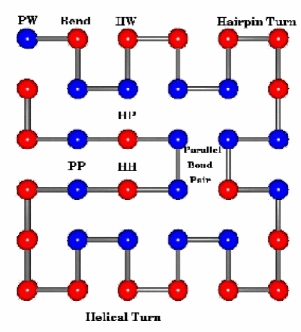
Figure 1: A 2-d model of a finite protein on a square lattice. The red spheres represent hydrophobic sites and the blue spheres represent hydrophilic sites.

III.1 Rooted or Anchored Protein

A proper model for protein folding will require using semiflexibility of the protein, for which we will use a recent model developed in our group GujSemiflex . It is the semiflexibility which gives rise to a crystalline phase; the latter represents the ordered native state of the protein at low temperatures. Therefore, we will treat a protein as a semiflexible self-avoiding copolymer chain on a lattice to study its folding by properly extending the above model GujSemiflex . The lattice is taken to be infinitely large ($N_{\text{L}}\rightarrow\infty$) so that the protein will never feel the effects of its boundary. Each amino acid residue (including any side group) is represented by a tiny sphere, which must lie on a lattice site; see Fig. 1. Each solvent also occupies a lattice site. We will consider an incompressible model so that no voids are allowed. A site is either occupied by a residue or by a solvent. The self-avoidance condition means that a lattice site cannot be occupied by more than one residue or a solvent. We consider a two-state model Dill ; Dill1999 in which each amino acid is classified either as a hydrophobic site (red spheres in Fig. 1 and denoted by H) or a hydrophilic/polar site (blue spheres in Fig. 1 and denoted by P). Due to the chemical structure of an amino acid, a protein is directional. One end of the protein has a free carboxyl group and is known as the C-terminus or carboxyl terminus. The other end of the protein has a free amino group and is known as the N-terminus or amino terminus. Proteins are always biosynthesized from the N-terminus to the C-terminus. On the other hand, most chemically synthesized proteins grow from the C-terminus to the N-terminus. Thus, a proper model should account for this directionality. Accordingly, in this work, we will incorporate the directionality of the protein, and treat both ends as dissimilar. This condition can always be relaxed without much complication. Treating both ends dissimilar basically doubles the number of distinct conformations of the protein, without any useful implication for the way the entropy behaves.

III.1.1 Compact and Unrestricted Protein Conformations

In our enumeration, we only consider a square lattice in this work. We will consider a protein to have either no restriction on its allowed conformations, or restrict it to only take a compact form, which we take to be rectangular. In the former case, the protein will be allowed to take all shapes including compact shapes by having it probe all allowed sites on an infinite lattice. In the second case, the protein will be restricted to have only compact shapes so that there are no solvent molecules in its interior; the surrounding of a compact region will be occupied by the solvent, i.e., water. The compact conformations are also present in the former unrestricted case. We will say that the conformations are unrestricted in the former case and compact in the latter case. In both cases, the end of the protein is rooted and is not allowed to move. There is a simple reason for rooting or anchoring the protein. The process of folding in vivo often begins co-translationally, so that the N-terminus of the protein begins to fold while the C-terminal portion of the protein is still being synthesized by the ribosome. Thus, it is the C-terminus that we root or anchor at the origin, and allow the N-terminus to be free to begin folding.

To generate compact rectangular shapes, we allow all possible rectangular shapes that could accommodate a given protein of size $M$. We give an example to clarify this point. Consider $M=24.$ For this case, we consider the following rectangular shapes in two dimensions: $1\times 24,2\times 12,3\times 8,$ and $4\times 6$. We do not need to separately consider $24\times 1,12\times 2,8\times 3$, and $6\times 4$ because of the rotational symmetry.

The anchoring has three important consequences for our computation. In the first place, this reduces the number of conformations that need to be counted. On an infinite lattice, an unanchored protein can start from any of the infinite lattice sites, making $W$ infinitely large. This trivial infinity due to nonanchoring has no bearing on thermodynamics. In the second place, anchoring allows us to uniquely define the distance between two conformations as we will discuss below. From now on, we will always root our protein at one of its ends on the lattice. In addition, we will also restrict the protein conformations so that its first bond from the root is along a fixed direction, which we take to be to the right, to limit the number of conformations. In order to further reduce the number of distinct conformations, we also restrict the first bend, as we start from the root, to be in the down direction of the square lattice. It is easily seen that any other conformation of the protein is related to one of the generated conformations by some trivial rotation. The last consequence of rooting is the following. There will be no doubling of conformations due to directionality that was discussed above.

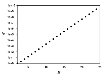
Figure 2: The rapid growth of $W$ (shown in the common log scale) with $M$ for an unrestricted protein on an infinite lattice. The allowed conformations are grown as described in the text.

The number of conformations $W$ for rooted proteins increases rapidly with the protein size, as is seen in Fig. 2. The number of conformations $W$ for rooted proteins increases rapidly with the protein size, as is seen in Fig.2 below. The growth of $W$ for the rooted protein with its first bond in a specified direction on an infinite lattice can be fitted by

$$W=0.102272\exp(0.990933M),$$

with $R^{2}=0.999876$ note2 . Correspondingly, the time required to generate all the conformations $W$ (but no other computation such as their energies, distances, etc.) also increases rapidly with the size $M$ as the following Table III.1.1 shows. The time reported here is on a PC. The time obviously increases if other computations are also carried out.

$$\text{Table \ref{Table_1}}-\text{Size and Computation Time on a PC}$$

III.2 Microscopic Interaction Energies

To account for the presence of water surrounding the protein, water molecules (to be denoted by W) are also allowed in the model. Each water molecule occupies a site of the lattice. To incorporate compressibility, voids can also be incorporated in the model. In that case, each void will be allowed to occupy a site of the lattice. We now turn to the complications induced by the compressibility.

III.2.1 Simplification Resulting from Incompressibility

Each conformation of the protein on the lattice results in certain sites of the lattice being occupied by the protein. In the incompressible model, rest of the sites will be occupied by the solvent. Thus, each conformation of the protein is associated with only one possible distribution of the solvent molecules on the lattice. Accordingly, there exists one and only one microstate of the system (the lattice containing the rooted protein) for each conformation of the protein. In other words, the number of possible microstates of the entire system is the total number of conformations $W$ of the rooted protein. It should be stressed that for sufficiently large volume $V$ or $N_{\text{L}}$ compared to $M$, the number of conformations $W$ will depend only on $M$ but not on $V$ or $N_{\text{L}}.$ This is a major simplification. The Gibbsian definition (14) of the entropy of the system refers to the sum over the microstates of the system. This means that the sum in (14) for the system is nothing but the sum over the conformations belonging to $W$.

This simplification is lost if we consider a compressible model containing voids. Then, there will be many more possible distributions of the solvent for each conformation of the protein. Let $k$ denote one of the microstates of the system, and $k(\Gamma)$ the set of microstates that are associated with a conformation $\Gamma$ of the protein. The set $k(\Gamma)$ depends not only on $M$ as above, but now it also depends on $N_{\text{L}}$ and $N_{0},$the number of voids, even if $N_{\text{L}}$ is sufficiently large. This is very different from the situation above for the incompressible limit. The entropy of the system is now given by the Gibbsian definition

$$S(T)=-{\displaystyle\sum}p_{k}\ln p_{k},$$ (16)

where $p_{k}$ is the probability of the $k$th microstate. This entropy can be reexpressed as follows:

$$S(T)=-{\displaystyle\sum_{\Gamma}}\sum_{k\in k(\Gamma)}p_{k}\ln p_{k}.$$

The number of microstates of the system which determine the sum in the Gibbsian definition (16) will far exceed the sum $W$ of protein conformations. This will make the computation much more extensive, depending on the amount of free volume (i.e. of the voids): larger the free volume, more extensive the computation. Because of this complication, we only deal with the incompressible model in this work.

III.2.2 Equal Size Approximation for Residues and Solvent

We do not allow voids in the present work, and take the solvent (water) molecule and the residue each to occupy a lattice site. This is an approximation as the water molecule and the residue do not have the same size. In a more realistic model, the water molecule and a residue may be allowed to occupy more than one lattice sites, depending on their relative size. While we can incorporate size difference in our lattice model, it makes the calculation harder. To avoid this, we adopt the simplification of equal size in this work.

III.2.3 Interaction Energies

The excluded-volume effects are accounted by enforcing that a lattice site cannot be occupied by more than one residue or water molecule. The interaction energies are restricted between chemically unbonded particles (residues H and P, and water molecules W) that are nearest neighbors of each other. Long range interactions are neglected, but can be incorporated later if so desired. We will not do that here. There are three species of particles (H,P, and W) in our model. As shown elsewhere Guj2003 , we need to only consider three independent energies of interaction between three chemically unbonded pairs of species. We have decided to use the following three van der Waals energies $e_{\text{HH}},$ $e_{\text{HW}},$ and $e_{\text{PH}}$ between the three unbonded pairs HH, HW, and PH. In the standard model due to Lau and Dill, only the first one in non-zero, as shown in Table III.2.3. To account for the semiflexibility of the protein, we use the model recently developed by us to study crystallization and glass transition in polymers GujSemiflex , but extend it to include preference of helical formation. The original model has a penalty $e_{\text{b}}>0$ for making a bend, an attractive energy $e_{\text{P}}<0$ between two parallel protein bonds, an attractive energy $e_{\text{hp}}<0$ for a hairpin turn (on top of the penalty for two consecutive bends in the same circulation direction), and an attractive energy $e_{\text{hl}}<0$ for a helical turn (on top of the energy for four bends and two hairpin turns).

We consider a protein with $M$ residues in a given sequence $\chi$ of H and P associated with the residues on a square lattice, with one of its end fixed at the origin so that the total number of conformations $W$ for a small protein remains finite even on an infinite lattice. We only consider the case in which the number of H and P are equal. This can be considered as the condition of charge neutrality. We generalize a recent model GujSemiflex , in which the number of bends $N_{\text{b}},$ pairs of parallel bonds $N_{\text{p}},$ and hairpin turns $N_{\text{hp}}$ characterize the semiflexibility; see Fig.1, where we show a protein in its compact form so that all the solvent molecules (W) such as water are expelled from the inside and surround the protein. The dark spheres denote hydrophobic residues (H) and light spheres denote hydrophilic (i.e., polar) residues (P). The nearest-neighbor distinct pairs PP, HH, HP, PW and HW between the residues and the water are also shown, but not the contact WW. Only three out of these six contacts are independent on the lattice Guj2003 , which we take to be HH, HW, and HP pairs. A bend is where the protein deviates from its collinear path. Each hairpin turn requires two consecutive bends in the same direction (clockwise or counterclockwise); see Fig. 1. Two parallel bonds form a pair when they are one lattice spacing apart. We also use the number of helical turns $N_{\text{hl}}.$ On a square lattice, a ”helical turn” is interpreted as two consecutive hairpin turns in opposite directions as shown in Fig. 1. The corresponding energies are $e_{\text{b}},$ $e_{\text{P}},$ $e_{\text{hp}}$, and $e_{\text{hl}},$ respectively. The interaction energies are $e_{\text{HH}}=-1,$ $e_{\text{HW}},$ and $e_{\text{HP}},$ corresponding to the HH, HW, and HP, respectively. The number of these pairs are $N_{\text{HH}},$ $N_{\text{HW}},$ and $N_{\text{HP}},$ respectively. We let $\mathbf{e}^{\prime}$denote the set containing all $\left\{e_{i}\right\},$ except $e_{\text{HH}}=-1,$ and $\mathbf{e}$ the entire set $\{e_{i}\},$where $i$ stands for b,p,hp,hl,HH,HW, and HP. Thus, $\mathbf{e,e}^{\prime}$ represent the sets

$$\mathbf{e} \equiv\left\{e_{\text{b}},e_{\text{P}},e_{\text{hp}},e_{\text{hl}},e_{\text{HH}},e_{\text{HW}},e_{\text{PH}}\right\},$$

$$\mathbf{e}^{\prime} \equiv\left\{e_{\text{b}},e_{\text{P}},e_{\text{hp}},e_{\text{hl}},e_{\text{HW}},e_{\text{PH}}\right\}.$$

Similarly, $\mathbf{N}\equiv\mathbf{N}(\Gamma)\equiv\{N_{i}(\Gamma)\}$ denotes the set

$$\mathbf{N}\equiv\left\{N_{\text{b}},N_{\text{P}},N_{\text{hp}},N_{\text{hl}},N_{\text{HH}},N_{\text{HW}},N_{\text{PH}}\right\},$$

and $\mathbf{N}^{\prime}$ denotes all $\left\{N_{i}\right\},$ except $N_{\text{HH}}:$

$$\mathbf{N}^{\prime}\equiv\left\{N_{\text{b}},N_{\text{P}},N_{\text{hp}},N_{\text{hl}},N_{\text{HW}},N_{\text{PH}}\right\}.$$

Let $W(\mathbf{N})$ denote the number of protein configurations on a lattice of size $N_{\text{L}}\geq M$. The energy of the configuration $\Gamma$ corresponding to the set $\mathbf{N}$ is given by

$$E(\mathbf{N})=\mathbf{e\cdot N=}\sum_{i}e_{i}N_{i}.$$ (17)

The energy varies from configuration to configuration as it depends on $\mathbf{N}$. But it does not depend on thermodynamic state parameters such as the temperature, pressure, etc.

The dimensionless entropy function corresponding to configurations with a given $\mathbf{N}$ is defined as

$$S(\mathbf{N})\equiv\ln W(\mathbf{N}).$$ (18)

(This definition amounts to setting the Boltzmann constant equal to 1.) There will in general be many sets $\mathbf{N}$ that will result in the same energy $E.$ We denote the collection of these sets by $\mathbf{N}(E).$ Thus, the number of configurations $W(E)$ for a given $E$ is obtained by summing $W(\mathbf{N})$ over this collection $\mathbf{N}(E):$

$$W(E)=\sum_{\mathbf{N}\in\mathbf{N}(E)}W(\mathbf{N}).$$ (19)

The corresponding entropy function for a given $E$ is given, as usual, by (5). The total number of all protein configurations, regardless of the energy $E$, is given by (2).

III.3 Various Model Energetics Choices

The three choices we have most often made for energies are described below in the form of three different models, the parameters for which are shown in Table III.2.3.

$$\text{Table \ref{Table_2}}-\text{Possible Models and their parameters}$$

III.3.1 Model (A)

In the standard model, the set $\mathbf{N}$ contains only one quantity, the HH contact number $N_{\text{HH}}.$ Thus, $\mathbf{e}^{\prime}=0,$ and the adimensional energy in this model is simply given by $E=N_{\text{HH}}.$ As $N_{\text{HH}}$ is going to be an integer, the corresponding density

$$n_{\text{HH}}\equiv N_{\text{HH}}/M$$

is going to be a discrete quantity, so will be the adimensional energy density $e\equiv E/M=n_{\text{HH}}$. The number of conformations $W(N_{\text{HH}})$ of a given $N_{\text{HH}}$ is

$$W(N_{\text{HH}})\equiv{\textstyle\sum}W(N_{\text{HH}},\mathbf{N}^{\prime}).$$ (20)

In the standard model, $E=N_{\text{HH}}$. It is clear from (20) that the entropy $S(N_{\text{HH}})=\ln W(N_{\text{HH}})$ for a given $N_{\text{HH}},$ regardless of $\mathbf{N}^{\prime}$, is maximum in the standard model Gujrati1 ; Guj0412548 . This feature of the standard model entropy is a possible justification of the observation made in Kolinski . As a consequence, the protein with a given $N_{\text{HH}}$ will probe many more states in the standard model than in any other model, which then slows down its approach to the native state. Thus, it is important to have non-zero $\mathbf{e}^{\prime}$ to step up the approach to the native state. (It is highly likely that the native states in different models are different, but this does not affect the above conclusion, provided the native states are unique.) There is another important consequences of having the remaining $\varepsilon_{i}=0.$ The fluctuations in the corresponding $N_{i}$ are maximum as there is no penalty no matter what $\mathbf{N}^{\prime}$ is. Hence, the protein will spend a lot of time probing a large number of conformations so as to maximize fluctuations in $\mathbf{N}^{\prime}.$ This also suggests that we need to go beyond the standard model to describe proteins that fold fast. Correspondingly, the entropy per residue is also discrete, with two successive values differing in the argument by $1/M.$ In other words, for small proteins, the entropy per residue $s(e)$ is not a continuous function, but a set of discrete values, as shown in Figs.4 and 5. It is clear from the figure that one can easily draw a concave envelop for the discrete values of $s(e).$ However, one can also draw a variety of other envelop functions that would not necessarily be concave such as those shown by the lines joining these points in the figures.

III.3.2 Weakly Perturbed Model (B₁,B₂)

In this model, we allow for other energies to be non-zero, but still small compared in strength. The model with the parameters in the above table will be called B₁ in the following. Another common choice we have made is $\mathbf{e}^{\prime}=(3/56,-1/56,-3/56,-3/56,21/56,5/56),$ and the corresponding model will be called B₂ in the following. The two models collectively will be simply denoted by B. The numerator of various energies are integers and are used to determine the energy $E$ as an integer, which makes it easy to classify energy levels in groups of a given energy. The energy is divided by the denominator at the end to ensure that $e_{\text{HH}}=-1.$ The energy corresponding to a HW-contact is the only energy close to $\left|e_{\text{HH}}\right|;$ this is to account for the strong repulsion between H and W. Otherwise, all other energies are extremely small compared to $\left|e_{\text{HH}}\right|.$ Consequently, this model will be identified as a model with weak perturbation on the standard model.

The model B₂ can also be treated as a model with small perturbations on the model B₁ (or vice versa) in which each residue is allowed to move about within the small cell surrounding the lattice site on which it is located. Such a disturbance will usually cause a small perturbation of B₁ (or vice versa) and can be described by the model B.

III.3.3 Strongly Perturbed Model (C₁,C₂)

In this model, we allow for other energies to be not only non-zero, but also comparable in strength to $e=1$. The most common choice we have made is the one shown in the Table III.2.3: $\mathbf{e}^{\prime}=(\ b,-b,-b,-b,2b,b),b=1/3(\simeq 1).$ We will call this the model C₁. Again, the numerators for various energies are integers for the reason explained above. Another model called C₂ has only one non-zero element $e_{\text{b}}=1$ in $\mathbf{e}^{\prime}.$ Both models will be collectively denoted simply by C.

The model A is the standard model. In the model B, we have most other interactions much weaker than $\left|e_{\text{HH}}\right|$, while they are comparable to $\left|e_{\text{HH}}\right|$ in the model C. Thus, the model B is closer to the model A than to the model C is. Despite this, we will see that the models B and C behave very different from A. It should be noted that $W$ does not depend on the model; it is its partition into $W(E)$ that depends on the model. Thus, the shape of the energy landscape changes from model to model, but not its total ”area” which is given by $W$ Guj0412548 .

III.4 Absence of Energy Gap

III.4.1 Semiflexible Homopolymers and Absence of Energy Gap

The semiflexibility of homopolymers has been exploited by Flory to explain crystallinity by using a very simple model, which contained only the bending penalty Flory . The energy was simply given by

$$E_{\text{Flory}}=e_{\text{b}}N_{\text{b}}.$$

No other interaction such as with the solvent was considered. Thus, the lowest energy is $E_{\text{Flory}}=0.$ At absolute zero, the polymer chains are going to be all straight with no bends (provided the chains are finite in length). Thus, it is anticipated that they would give rise to an ordered structure. One possibility is that of an aligned configuration in which all chains are parallel to each other, though this is by no means the only configuration as one can envision many other configurations of the same energy $E_{\text{Flory}}=0.$ The aligned configuration was considered by Flory to represent the crystalline state formed by linear polymers. Thus, it is expected that the above simple model will give rise to a melting transition from a disordered liquid state to a crystalline state at a melting temperature $T_{\text{M}}$.

To make connection with our protein model, we will henceforth consider the limiting case of a single macroscopically large semiflexible homopolymer chain. The original approximate solution due to Flory indeed shows such a melting transition at a non-zero melting temperature $T_{\text{M}}$. The approximation used by Flory gives rise to an energy gap, which is deduced by the observation that the resulting entropy based on the approximation becomes negative over the gap, similar to what happens in the random energy model discussed earlier in Sect. II.5. Over the gap, the entropy is replaced by $S(E)=0;$ we will use $E$ instead of $E_{\text{Flory}}$ in the following for convenience. This gap then makes the entropy non-concave and results in a melting transition in the model. The transition turns out to be a freezing transition in that the entropy of the frozen state (the crystal) remains zero below the melting temperature, just as was the case for the random energy model.

It was later shown by Gujrati and coworkers GujGoldstein that there was no energy gap in the Flory model of semiflexible homopolymers. A macroscopic chain with no solvent was considered. For the infinitely long polymer chain in the absence of any solvent, the problem is also known as the Hamilton walk problem, the problem in which the walk visits all sites once and only once. The demonstration of the absence of an energy gap was achieved by demonstrating that the entropy was never negative over the entire energy range in the model. The demonstration itself was done by obtaining a rigorous lower bound to the entropy $S(E)$. This required an explicit construction in which local excitations, the Gujrati-Goldstein excitations (GG excitations) which are pairs of oppositely oriented hairpin turns, populate the crystal. One such excitation is shown in Fig. 1 for the case of no solvent in the interior. It is the local excitation represented by the two hairpin turns where the parallel bond pair is shown in the figure: it is a ”bound” pair of oppositely oriented hairpin turns and represents a GG excitation. These GG excitations should be distinguished from unpaired hairpin turns. The unpaired hairpin turns either cannot be moved, or can be moved only by changing the number of bends or of parallel bonds or by introducing voids; see the hairpin turn in the second row (from the top) just above the shown HP pair in Fig. 1; it cannot be moved up or down without increasing the number of bends or of parallel bonds or by introducing voids. In contrast to these, the bound GG excitations are highly ”mobile” in that they can be moved about without changing the number of bends or of parallel bonds or by introducing voids until they hit another defect or the wall; see the excitation between the third and fourth row (from the top) in Fig. 1, which can be freely moved to the left. This ”agility” of the excitation increases the entropy in the system without changing the energy in the model. It should be noted, see Fig. 1, that an isolated hairpin turn can be turned into a GG excitation by increasing the number of bends by 4 and parallel bonds by 2, after which the excitation becomes ”agile” to move.

The distances over which the GG excitations can be moved can be easily estimated in a crude fashion by the defect density. This is similar to the interparticle distance between particles at a given concentration $c$, which is given by $c^{-1/d}$, where $d$ is the dimension of the lattice. We can use for $c$ the density $c_{\text{d}}$ of the defects (the bends, hairpin turns or the GG excitations) in the crystal. Thus, the number of possible moves for a single GG excitation is this distance and is on an average

$$W_{\text{GG}}\sim c_{\text{d}}^{-1/d}/a=c_{\text{d}}^{-1/d},$$ (21)

as we have set $a=1$. At $T=0,$ we surely have $c_{\text{d}}=0.$ The GG excitations along with other defects like the bends, the hairpin turns, etc. gradually populate and begin to destroy the perfect crystalline order by increasing the entropy as soon the temperature rises above $T=0,$ and the crystalline phase melts at the melting (or unfolding) temperature $T_{\text{M}}$ into a disordered phase GujSemiflex . The crystalline state has been shown to occur via a sharp first-order transition if we have either an infinitely long macroscopic polymer GujGoldstein or a bulk system containing a macroscopic number of finite length polymers GujSemiflex provided we allow other energies besides that for bending. As long as we have a single polymer, which is finite in length, the folding transition is not going to be sharp, but diffuse.

III.4.2 Semiflexible Copolymer and Absence of Energy Gap

The constructive proof of no energy gap also works for the current protein model, as we now discuss. The main difference is that while the calculation discussed above for the homopolymer is done rigorously, we do not have a rigorous calculation at present for the copolymer because of the complexity produced by the sequence structure. Our results are based on plausibility arguments, which we present below. As said earlier, the issue of an energy gap in proteins requires studying macroscopic proteins. We, therefore, consider a single macroscopic protein. We will also not consider any solvent, so that we are dealing with a Hamilton walk problem. Accordingly, $M=N_{\text{L}},$ and $c=1/a=1$. As we have just seen, the presence of the Gujrati-Goldstein excitations in a homopolymer implies that there is no energy gap in our model of melting for a homopolymer GujGoldstein ; GujSemiflex . We now extend the constructive proof to the copolymer case (or to the heteropolymer case). The complication arises from the presence of other interactions, such as the HH interaction. Let us for the moment only consider the bending penalty and the hairpin and parallel bond energies in addition to the contact interaction energy due to the HH pair contacts. Thus, we consider the variant models B and C and not the standard model in the following. We will return to the standard model later.

Consider a macroscopically large copolymer of a given sequence $\chi$ on a lattice. Let us consider the native state at $T=0.$ The attractive HH interaction and a favorable (negative) energy for a hairpin turn compete with the bending penalty in order to minimize the internal energy in the native state. In contrast, one only need to maximize the HH contact number without any regard to the number of bends in the standard model, and to only minimize the number of bends in the Flory model without any regards to the HH contacts. We will assume that there is only one unique native state (modulo any symmetry operation). For example, for $M=24,$ we show the native state for the model B₁ in (32), which is related to the native state in (34) by a symmetry transformation (30) as explained later. This does not prove but strongly suggests a unique native state even for larger $M$.

Because of the favorable nature of hairpin turns, the native state must have a non-zero density of them. Thus, the defect density $c_{\text{d}}$ would be non-zero at $T=0,$ which makes this problem inherently different from that of the semiflexible homopolymer. Some of the hairpin turns must be in the bound state in the form of the GG excitations. We assume that there is a non-zero density $c_{\text{GG}}$ of these excitations in the native state at $T=0$. The native state will usually have the maximum number of the HH contacts for most of the sequences $\chi$ as $e_{\text{HH}}$ has the maximum strength. If we move a GG excitation, this will require a rearrangement on the lattice of that portion of the protein that is contained between the two hairpin turns of the excitation under investigation. We can crudely estimate the number of residues on this portion of the protein as

$$n_{\text{R}}\sim M/c_{\text{d}}V=1/c_{\text{d}}a^{d}=1/c_{\text{d}}.$$

Half of this number is the average number of H residues in this portion.

The positions on the lattice of the residues belonging to this portion of the protein will change with the movement of the GG excitation. Even though this movement does not change the number of bends and parallel bonds, it will invariably reduce the number of HH contacts compared to that in the native state. Thus, the energy of the deformed conformation due to the GG excitation movement will be higher than that of the native state. Indeed, this is true of any deformation of the native conformation (including that generated by the movements of the GG excitations): Any deformation of the native state will always raise the energy since by definition, the unique native state has the lowest energy (at $T=0$). For the deformation due to the GG excitation movement, this increase is due to breaking some of the HH contacts.

Not much can be said about how much the increase in the energy will happen in displacing a GG excitation, as it depends strongly on the sequence $\chi$ and on the topology of the native state. Furthermore, not all newly generated conformations in $W_{\text{GG}}$ will have the same excess energy. We now pick an extensively large number of GG excitations and move each of them, which results in $W_{\text{GG}}$ new conformations. The new $W_{\text{GG}}$ is the product of $W_{\text{GG}}$  in 21 over the set of selected GG excitations in the construction. The resulting gain in the entropy density will be

$$\Delta s\sim(n_{\text{GG}}/d)\ln c_{\text{d}},$$

where $n_{\text{GG}}$ is the density of GG excitations used in the construction. We expect $n_{\text{GG}}$ to be proportional to the defect density $c_{\text{d}},$ at least for small $c_{\text{d}},$ so that the above entropy gain vanishes as $c_{\text{d}}\rightarrow 0$.

Let $W_{\text{GG}}(E)$ denote the number of conformations in the above construction to have the energy $E,$ where $E>E_{0},$ $E_{0\text{ }}$being the energy of the native state. Obviously,

$$W_{\text{GG}}\equiv\sum_{E}W_{\text{GG}}(E),$$

where the sum is over possible energies that appear in the construction due to the movement of the excitation. For a macroscopic system, the sum is going to be dominated by some energy $E=\overline{E}>E_{0},$ so that

$$W_{\text{GG}}\simeq W_{\text{GG}}(\overline{E}).$$

But a little reflection will convince the reader that the excess energy density $\overline{e}-e_{0}$ is also proportional to $n_{\text{GG}}.$ Thus, we will obtain a continuous energy density spectrum in our construction. As the construction only generates some of the conformations of energy $E=\overline{E},$ the actual entropy gain is at least as much as $\Delta s>0$ given above. Consequently, it does not seem possible to have an energy gap for most of the sequences.

IV Self-Averaging and Small Proteins

For a system with quenched randomness, which in our case is created by the fixed sequence of amino acids, an important question about self-averaging has been probed. The idea is quite simple. Consider a protein with $M$ amino acids in a given sequence $\chi.$ The sequence for a given protein is fixed in Nature (or in the lab, where it is synthesized). However, there are several possible sequences. For example, consider all possible sequences for any given $M$ in which there are exactly $s$ H-type residues and $(M-s)$ P-type residues. The number of possible distinct sequences is given by

$$C_{M,s}\equiv\frac{M!}{s!(M-s)!}.$$

On the other hand, if we consider all possible sequences without any restrictions on the number of H-residues, then the number of possible sequences is $2^{M}$ corresponding to all possible values of $s.$ The most probable value of $s$ is $s=\left[M/2\right],$ where $\left[x\right]$ is the integer part of $x,$ since $C_{M,\left[M/2\right]}$ is maximum. Let us denote the set of corresponding sequences by $\widetilde{\boldsymbol{\chi}}$. Loosely speaking, we will call these sequences the most probable sequences, knowing well that it is the value of $s$ or the corresponding set $\widetilde{\boldsymbol{\chi}}$ that is most probable and not one of the sequences.

Let $Q$ denote a certain thermodynamic property like the energy of the native state, the free energy of the protein, the number of helices in the native state, etc. This quantity will, in general, depend on the sequence $\chi,$ and one can determine its quenched average

$$<Q>_{\text{seq}}\equiv\frac{1}{\left|\chi\right|}\sum_{\chi}Q(\chi),$$ (22)

where $\left|\chi\right|$ is the number of possible sequences over which the averaging is done. The property $Q$ is said to be self-averaging if

$$\lim_{M\rightarrow\infty}Q(\chi)=\lim_{M\rightarrow\infty}<Q>_{\text{seq}}$$ (23)

for almost all $\chi$. As usually happens in the thermodynamic limit, $\widetilde{\boldsymbol{\chi}}$ contains almost all the sequences. This is evident from the behavior of  $C_{M,s}$ for large $M$. The most probable sequence contains $C_{M,\left[M/2\right]}\simeq 2^{M}$ for $M>>1.$ This is also the number of all sequences. Then, the above condition of self averaging really refers to any sequence belonging to $\widetilde{\boldsymbol{\chi}}.$ It is clear that the idea of self-averaging, which is not a trivial property, requires considering a macroscopic copolymer. If the property is self averaging, then the limit on the left in (23) is independent of the sequence $\chi$. This important property then gives rise to many simplifications. For example, it allows one to use the replica trick ReplicaTrick to calculate the quenched averages of quantities such as the free energy. The trick represents a major technical advantage that has been extensively used quite successfully to study macroscopic random systems. As shown in Kardar , there are strong indications that self averaging is valid for macroscopic proteins.

It is instructive now to see how well the equality (23) (without the limits on both sides) is obeyed for finite $M$. For this purpose, we consider the native state energy $E_{0}$ to be the the thermodynamic property $Q,$ and consider the quenched average of the native state energy density $e_{0}\equiv E_{0}/M$:

$$<e_{0}>_{\operatorname{seq}}\equiv\,\frac{1}{M}<E_{0}>_{\operatorname{seq}}\equiv\frac{1}{M\left|\chi\right|}\sum_{\chi}E_{0}(\chi)$$

over all sequences that belong to $\widetilde{\boldsymbol{\chi}},$ so that the average is taken over all sequences with the restriction of equal H and P (even $M$). Thus, not all sequences are allowed. This is done because of the importance of the most probable sequence noted above and requires evaluating $E_{0}(\chi)$ for each sequence in $\widetilde{\boldsymbol{\chi}}.$

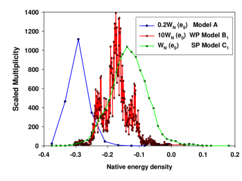
Figure 3: The scaled distribution of $\widetilde{W}(e_{0})$ as a function of the native state energy $e_{0}$ for 10,000 different sequences for unrestricted coformations of $M=24$. For the standard and the weakly perturbed models, we show the scaled distribution $\widetilde{W}(e_{0})/5$ and $10\widetilde{W}(e_{0})$ so that the scaled distributions can be shown on the same scale.

Let $W_{\text{N}}(e_{0})$ denote the number of times a given native energy $e_{0}\equiv E_{0}/M$ appears among all sequences in $\widetilde{\boldsymbol{\chi}}$. We then calculate the relative root mean square (rms) fluctuation

$$\,\left\langle\delta e_{0}\right\rangle_{\text{seq}}\equiv\frac{\sqrt{<e_{0}^{2}>_{\operatorname{seq}}-(<e_{0}>_{\operatorname{seq}})^{2}}}{\left|<e_{0}>_{\operatorname{seq}}\right|},$$ (24)

where

$$<e_{0}^{2}>_{\operatorname{seq}}\equiv\frac{1}{M\left|\chi\right|}\sum_{\chi}E_{0}^{2}(\chi).$$

Standard arguments ReplicaTrick show that the relative fluctuation $\left\langle\delta e_{0}\right\rangle_{\text{seq}}$ should decrease as $1/\sqrt{M}$ for large $M$:

$$\left\langle\delta e_{0}\right\rangle_{\text{seq}}\propto 1/\sqrt{M}.$$ (25)

We have done the calculations for the three models for $M=16,$ and $M=24$ on an infinite lattice. For $M=16,$ we have considered all the sequences in $\widetilde{\boldsymbol{\chi}}$, each with equal number of H and P residues. The total number of these restricted sequences is

$$C_{16,8}=12,870.$$

For $M=24$, we have only considered $10,000$ different sequences for the three different classes of energetics, which is a small fraction of all allowed sequences $C_{24,12}=2,704,156.$ We only show the distribution for $M=24$ in Fig.(3). The results for various quenched averages and the relative fluctuations are summarized in Table IV.

$$\text{Table \ref{Table_3}}-\text{Quenched averages and relative fluctuation}$$

We see that the relative fluctuation increases as the strength of the perturbation increases for both sizes. In addition, it appears that the relative increase ($0.4320/0.1079=3.8519$ for $M=16$) or ($0.6448/0.1674=4.0037$ for $M=24$) does not appreciably change with the size. This needs to be investigated further for other sizes. Moreover, the relative fluctuation is not small, implying that the spread of the distribution $W_{\text{N}}(e_{0})$ is not insignificant. If we calculate $\sqrt{M}\left\langle\delta e_{0}\right\rangle_{\text{seq}}$ from Table IV, we observe that this product is much smaller for $M=24$ than for $M=16,$ while according to (25), this product should not change. There are two possibilities for this behavior. It is quite conceivable that either $M=24$ is not large enough for (25) to be observed or that the choice of only $10,000$ sequences for $M=24$ does not give a good estimate of the relative fluctuation $\left\langle\delta e_{0}\right\rangle_{\text{seq}}.$ Thus, our results may not be reliable enough to prove or disprove self-averaging for a macroscopic protein. Nevertheless, the results in Table IV for the small proteins that we have considered in the present work clearly show that the average native state energy $<e_{0}>_{\operatorname{seq}},$ though highly probable, does not represent the native state energy of almost most of the random sequences in $\widetilde{\boldsymbol{\chi}}.$ There is no reason to believe that other thermodynamic quantities will have their sequence average equal the average of any randomly selected sequence. Thus, small proteins are not self-averaging. This is consistent with the accepted result in the literature, see for example, Bryngelson , that sequences play an important role in small proteins.

The situation in Fig.(3) does raise an interesting question. We see the most probable native energy is far from the lowest native energy for each of the three models. Does Nature prefer to design proteins whose native energies are close to the most probable native energies or to the lowest native energy? It should be remarked that all those sequences that have their native energies close to the most probable native energy do not fold into one unique native structure, though many sequences are found to have the same structure (conformations without any regard to the sequence). The native conformations, though compact, have varied structures.

For the standard model in Fig.(3), we observe that there are eight different native energies for the $10^{4}$ random sequences for the standard model. We find that $e_{0}\simeq-0.3$ is the most common native state energy; all these native states differ only in their sequences. None of the models ascribes a unique structure of the native conformation to a particular sequence. However, the standard model does point to an interesting fact. The number of sequences with the lowest native energy $e_{0}\simeq-0.38$ is an extremely small fraction of the $10^{4}$ sequences considered here. It should be remarked that the sequence $\chi_{0}$ described below in 26 gives a much lower native state energy $e_{0}=-0.4167,$ and is not part of the $10^{4}$ sequences whose results are shown in Fig.(3). For $M=16,$ there are seven different native energies between $e_{0}\simeq-0.44$ and $e_{0}=0$ for the standard model. The most dominant native energy is $e_{0}\simeq-0.31$ given by $5664$ sequences, but the number of sequences with the lowest energy ($430$) is not as small a fraction as for $M=24.$ Thus, it appears that the fraction of sequences among all sequences that gives the lowest possible native energy is small, this fraction becoming smaller as the protein size increases. This suggests that the most probable native energy distribution becomes narrower with the size $M.$ This observation, which seems to support the emergence of self-averaging for $M\rightarrow\infty$, needs to be checked further.

For the weakly perturbed model, the same distribution $W_{\text{N}}(e_{0}),$ see Fig. (3), exhibits a clear band structure; the number of bands seems to be clearly controlled by the number of possible energies in the corresponding standard model. However, the band structure is ”smoothed out” for the strongly perturbed model because the latter does not allow as many native state energies as the weakly perturbed model. Because of this difference in the allowed native state energies, the maximum $W_{\text{N}}(e_{0})$ for the weakly perturbed model is much smaller than the maximum $W_{\text{N}}(e_{0})$ for the strongly perturbed  model.

We have found that in the majority of cases that we have investigated, the following sequence containing a repetition of PHHP and which we denote by $\chi_{0}$

$$\chi_{0}:(\text{PHHP})_{n}$$ (26)

gives rise to the lowest energy or very close to it. Because of this, we mostly present results based on this particular sequence $\chi_{0}$ in this work, though we have considered other sequences also.

V Energetics and Native Conformations

Let us fix $M=24$ and consider unrestricted conformations. The sequence is fixed to $\chi_{0},$ i.e. to

PHHPPHHPPHHPPHHPPHHPPHHP

for the reason explained in the preceding section. For the standard model, there are $30$ native states, all of the same energy density $e_{0}=-0.4167,$ as discussed in the following. One of the native states is the following conformation:

$$\begin{array}[c]{cccc}1\text{P}&2\text{H}&3\text{H}&4\text{P}\\ 8\text{P}&7\text{H}&6\text{H}&5\text{P}\\ 9\text{P}&10\text{H}&11\text{H}&12\text{P}\\ 16\text{P}&15\text{H}&14\text{H}&13\text{P}\\ 17\text{P}&18\text{H}&19\text{H}&20\text{P}\\ 24\text{P}&23\text{H}&22\text{H}&21\text{P}\end{array},$$ (27)

and can be represented by the string

RRRDLLLDRRRDLLLDRRRDLLL, (28)

which is read from the left and refers to the sequential steps from the first residue along the right (R), left(L), up (U), and down (D) directions. The first step is always to the right direction, and the first bend is always in the D direction. This is done to cut down the number of conformations to be counted. All conformations in which the first bend is in the U direction is topologically identical to one of the conformations that we generate. Similarly, conformations that start not in the R direction are also topologically not distinct. Despite these restrictions, we still duplicate some conformations if the two ends of the protein are treated identically. This happens when the last step of the protein is in the L direction and the bend before the last step is in the U direction. We will explicitly demonstrate this below. However, this does not affect us as we deal the two ends as different.

We also report the nine other native states that are given by the strings

$$\begin{array}[c]{c}\text{{\normalsize RRRDLLLDRRRDLLLDRRRDLLD,}}\\ \text{{\normalsize RRRDLLLDRRRDLLLDRDDRUUR,}}\\ \text{{\normalsize RRRDLLLDRRRDLDRDLLLURUL,}}\\ \text{{\normalsize RRRDLLLDRDLDRDDRUURULUR,\ }}\\ \text{{\normalsize RRRDLDRDLDRDLLLURULURUL,\ }}\\ \text{{\normalsize RRDLURDRURRULLULDLULDLL,\ }}\\ \text{{\normalsize RRDLURDRURRULLULDLULDLU, }}\\ \text{{\normalsize RDLDRRRULURURRRULLLURRR,\ }}\\ \text{{\normalsize RDLDRRRULURURRRULLLURRU.\ }}\end{array}$$ (29)

We notice that the third and the eighth strings above are related by

$$\text{L}\Leftrightarrow\text{R,U}\Leftrightarrow\text{D, and the reversal of the strings;}$$ (30)

an example is given below for clarity. Thus, there are only $9$ distinct native states if the two ends are treated identically. Of course, the above symmetry transformation does not affect our calculation since we make a distinction between the N-terminus and the C-terminus.

For the weakly perturbed model B₁, there are two native states of energy density $e_{0}=-0.3717$. The native state string

RRRDLDRDLDRDLLLURULURUL (31)

represents the following native state

$$\begin{array}[c]{cccc}1\text{P}&2\text{H}&3\text{H}&4\text{P}\\ 24\text{P}&23\text{H}&6\text{H}&5\text{P}\\ 21\text{P}&22\text{H}&7\text{H}&8\text{P}\\ 20\text{P}&19\text{H}&10\text{H}&9\text{P}\\ 17\text{P}&18\text{H}&11\text{H}&12\text{P}\\ 16\text{P}&15\text{H}&14\text{H}&13\text{P}\end{array}.$$ (32)

The other native state string

RDLDRDLDRRRULURULURULLL (33)

represents the native state

$$\begin{array}[c]{cccc}24\text{P}&23\text{H}&22\text{H}&21\text{P}\\ 1\text{P}&2\text{H}&19\text{H}&20\text{P}\\ 4\text{P}&3\text{H}&18\text{H}&17\text{P}\\ 5\text{P}&6\text{H}&15\text{H}&16\text{P}\\ 8\text{P}&7\text{H}&14\text{H}&13\text{P}\\ 9\text{P}&10\text{H}&11\text{H}&12\text{P}\end{array}.$$ (34)

This native state is topologically identical to the previous native state, and is described by the string obtained by the symmetry transformation (30), as noted above if the two ends are identical. It is clear that the weak perturbation alone has drastically reduced the native state multiplicity from $30$ to $2$. This shows the importance of even the weak perturbation.

The strongly perturbed model, surprisingly, has three native states given in (27),(32), and (34); the last two are related to each other by the above transformation. This suggests that the relationship between a given native state and the energetics is quite complex. The set $\mathbf{N}$ for the first two native conformations are $(10,15,5,0,10,4,0)$, and $(18,12,9,7,10,4,0)$; the third native conformation has the same $\mathbf{N}$ as the second one above, which should not come as a surprise. The energy density of each of the three native conformations is $(-32/72).$ If we use $e_{\text{hp}}=-2/3=e_{\text{h}},$ then only the last two conformations survive as the native conformations; the first one is no longer a native conformation. Now, the native energy density is $(-48/72),$ and $\mathbf{N}$ is $(18,12,9,7,10,4,0),$ the same as for the previous set of energetics. This is a clear demonstration of the fact that the same native state can occur in various different models. Therefore, one cannot determine effectively the energetics of a protein by only studying the native states. For this, one must also investigate many of the non-native conformations.

VI Small System Thermodynamics

VI.1 Microcanonical Entropy

VI.1.1 Equilibrium

The dimensionless ME entropy corresponding to configurations with a given energy $E$ is given by the Boltzmann relation (5); as above, we have set the Boltzmann constant equal to 1. This entropy is relevant if the energy of the protein is held fixed. Keeping $E$ constant is not the same as keeping each term $e_{i}N_{i}$ in the sum in (17) constant; the latter can change as long as the sum in (17) remains constant. We define the equilibrium to mean that the protein explores all possible conformations included in $W(E)$ with equal probability given in (12).

Let us recall the arbitrary positive energy $\epsilon$ (we can take this to be the magnitude $\left|e_{\text{HH}}\right|$ for concreteness) that we have used to introduce the adimensional energy $E,$ which is really $E/\epsilon$ note . For  a small protein ($M<\infty$), each element in the set $\mathbf{N}$ is finite. Thus, the adimensional energy is also finite, with the closest spacing $\Delta_{\text{min}}E$ between two successive values of $E$ at least $\left|e_{\text{min}}\right|$ (which is really $\left|e_{\text{min}}\right|/\epsilon$), where $e_{\text{min}}$ is the element with the smallest magnitude in the set $\mathbf{e.}$ Therefore, for small proteins, $E$ is a discrete variable. The corresponding energy density per residue

$$e\equiv E/M$$

is also discrete and becomes continuous only when $M\rightarrow\infty.$ Thus, as long as $M$ is finite, the energy and the entropy density per residue

$$s(e)\equiv S(E)/M$$

remain discrete. In addition, they also depend on $M$ for small proteins note01 . To show this most clearly, we reproduce $s(e)$ for the strongly perturbed model C₁ in Fig. 4 for $M=16,24,32,40$, and $48;$ we restrict the conformations of the protein to be compact. There continues to be a dependence on $M,$ even though the largest value of $M$ is $\ 48.$ We also note that the discrete nature of the energy and entropy persists. There is a clear evidence of many local maxima in the entropy, each maximum surrounded by many energies of lower entropy forming an energy band. These bands are well separated by gaps in the energy, at least near the low end of the energy even for $M=48.$ It is surprising to observe the erratic form of the entropy in that the bands are highly irregular in shape, at least near the low energy end. The entropy function is becoming somewhat smoother (but still discrete) near it global maximum because the energy levels are becoming denser in this range.

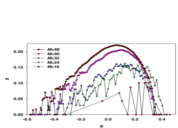
Figure 4: The behavior of $s(e)$ for the strongly perturbed model C₁ of a compact protein as a function of the protein size $M$. We observe that the both the lowest and the highest energy densities decrease with the protein size.

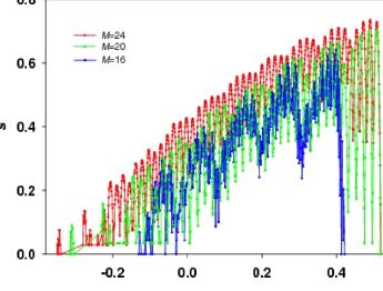
Figure 5: The behavior of $s(e)$ for the weakly perturbed model B₁ on an infinite lattice as a function of the protein size $M$. We observe that $s(e)$ for the larger size contains that for the smaller size inside it.

In Fig. 5, we show the ME entropy $s(e)$ when the protein conformations are unrestricted. We are considering a weakly perturbed model B${}_{1}.$ We again see a dependence of $s(e)$ on $M$, as before. Similarly, the allowed energy densities continue to depend on $M.$ This dependence is not so weak to be negligible, especially near the low energy range, the range more appropriate and influential in studying protein folding. This is a clear indication that one cannot treat the densities such as $s$, and $e$ to be independent of $M$. This point does not seem to be appreciated in the literature; see for example, Clementi1 . We notice that $s(e)$ remains discrete even for $M=24$, close to the largest protein we have investigated in the case when the conformations are unrestricted.

There are some common features in both figures 4 and 5. The first feature is the presence of gaps in bands of $s(e)$ at lower energies: there is a clear energy gap between the two lowest bands for $M$ ranging from $24$ to $48$ for compact conformations and for $M$ ranging from $20$ to $24$ for unrestricted conformations. The gap decreases with $M$ in both cases. This is consistent with the claim in Sect. III.4 of no energy gap in the model. Another feature we notice is that $s(e)$ is usually higher for larger $M$ over a wide range of energies. There is a certain pattern in the undulations present in $s(e):$ they seem to form a band structure with several peaks within each band; the number of peaks in a band keeps increasing with $M.$ The presence of these bands will be explained below.

The native state of the protein is, by definition, the lowest energy state at absolute zero. Depending on the interactions in the protein and the sequence $\chi$ of H and P residues in it, the native state may or may not be unique. In the latter case, the multiplicity of the lowest energy state will indicate that the protein functionality is not simply determined by the native state. (We will call this multiplicity the degeneracy of the native state.) The way out of this dilemma is to have the energetics tuned in such a way that the native state becomes unique. At present, our understanding of protein functionality is not so complete to answer this question unambiguously. Therefore, we will allow the occurrence of degenerate native states and study the effect of energetics on this degeneracy to learn how the energetics should be tuned to give a unique native state. It may be that there exist high energy barriers between these native states so that it is impossible for the protein to jump from one native state to another in a finite amount of time. However, it should be recognized that for a small protein ($M<\infty$), no energy barrier of any kind except due to excluded volume interactions (which occur when a site is occupied twice, but do not exist in our lattice model as only configuration satisfying excluded volume constraints are allowed) can be infinitely large; hence, the time required to transform from one native state to another will remain finite, though it may be large in some cases. Thus, this idea of a large barrier to explain the robustness of a protein may not be so reliable or relevant.

VI.1.2 Non-equilibrium

Away from equilibrium, the protein will not explore all the conformations in $W(E)$ with equal probability. In this case, the entropy of the non-equilibrium state is given by the Gibbsian relation (14) in which $p(\Gamma),$ where $\Gamma$ is one of the conformations in $W(E)$, is independent of the temperature. This non-equilibrium microcanonical Gibbsian entropy will eventually achieve its maximum under the constraint

$$\sum_{\Gamma}p(\Gamma)\equiv 1,$$ (35)

as the protein equilibrates. This is easily seen by the using the Lagrange multiplier trick to maximize the combination

$$\sum_{\Gamma}p(\Gamma)(-\ln p(\Gamma)+\lambda),$$

where $\lambda$ is the Lagrange multiplier. The resulting distribution is given by

$$p(\Gamma)=\exp(\lambda-1).$$

The use of (35) determines the Lagrange multiplier

$$\exp(\lambda-1)=1/W(E).$$ (36)

Thus, the resulting equilibrium distribution is given by the Boltzmann relation (5). This is the conventional law of increase of entropy in thermodynamics as the system moves towards equilibrium.

This formulation of the second law is obviously applicable to small systems such as our protein in our approach based on the Conjecture 3, and also justifies our Conjecture 1.

VI.2 Behavior of the Compact and Unrestricted Conformations

The behavior of $S(E)$ is different compact and unrestricted conformations. We first consider the standard model. For unrestricted conformations, the maximum energy corresponds to non-compact conformations of which there are many; the actual value depends on the value of $M.$ Thus, $S(E)$ does not vanish at the upper end of the energy. Here, the entropy continues to increase as the energy increases. This can be easily seen in Fig. 6. On the other hand, the situation is drastically different for compact conformations. Here, there are not that many configurations of the highest energy. Thus, the entropy first rises and then drops as the energy increases. This remains true for any of the three models, and we refer the reader to Fig. 4 where we have shown the results for compact conformations in the model C${}_{1}.$

Let us consider unrestricted conformations of the protein. The standard model entropy will be perturbed drastically even with weak perturbation of energies. This is because the number of conformations that contribute to $W(N_{\text{HH,max}})$ at the highest energy $E_{1}\equiv-N_{\text{HH,max}}$ in the standard model will redistribute themselves in a band due to weak energy perturbation. The spread of the band will now give zero or very small entropy at the highest energy in the two perturbed models. This causes a drastic change in the form of the entropy distribution: each energy level of the standard model turns into a band; see the bands of the perturbed models in Fig. 6. We see that there are exactly 11 bands, equal in number to the 11 energy levels in the standard model A. The energy gap between the bands at the low end of the energy spectrum in the weakly perturbed model is also a manifestation of the energy gap in the standard model. This gap is easy to notice in Fig. 5 where we have also shown the entropy at low energies for the model B${}_{1}.$ This gap seems to be almost filled up in the strongly perturbed model C; see Fig. 6.

As $M$ increases, the energy spectrum in $e$ becomes dense so that $e$ and, therefore, $s(e)$, become continuous.

VI.3 Canonical Partition Function

A protein in Nature is not a closed system as discussed above. Therefore, the ME is not the most suitable ensemble to investigate. As the protein interacts with its surrounding at a given temperature $T$, we need to consider the CE in which the temperature of the system and its surrounding is held fixed. This description is more realistic and can be characterized by the canonical partition function given by

$$Z(T)\equiv\sum_{E}W(E)\exp(-\beta E),$$ (37)

where $\beta\equiv 1/T$ is the inverse temperature in the units of the Boltzmann constant. The reader should be warned that we are using the partition function formalism, which is believed to give the correct thermodynamics of large systems, for the current case of a small protein. The thermodynamics of a small system is far from a complete understanding in that it is not known if the small system thermodynamics is the same as that predicted by the use of the above partition function (37). We will not be concerned with this issue here and adopt the most prevalent view in the field and use the above small-system partition function formalism to study the thermodynamics of the small system. A credible justification of this adoption will be provided at the end of the next section.

It is convenient to rewrite the partition function as a sum over $\mathbf{N}$ as follows:

$$Z(T)\equiv\sum_{\mathbf{N}}W(\mathbf{N})\exp[-\beta E(\mathbf{N})].$$

¿From this, we can calculate the thermodynamic averages $\overline{N_{i}}$ as follows:

$$\overline{N_{i}}\equiv\frac{\sum_{\mathbf{N}}N_{i}W(\mathbf{N})\exp[-\beta E(\mathbf{N})]}{Z(T)}=-\left(\frac{\partial}{\partial\beta e_{i}}\ln Z(T)\right),$$ (38)

where the derivative is taken at fixed $\beta\mathbf{e}_{i}^{\prime}$, where $\mathbf{e}_{i}^{\prime}$ represents the set of all the remaining energies in the set $\mathbf{e}$ except $e_{i}$, and may be a null set. If we introduce the fluctuation $\Delta N_{i}\equiv N_{i}-\overline{N_{i}},$ then

$$\overline{\left(\Delta N_{i}\right)^{2}}=\left[-\frac{\partial}{\partial\beta e_{i}}\right]^{2}\ln Z(T)=-\left(\frac{\partial\overline{N_{i}}}{\partial\beta e_{i}}\right)\geq 0.$$ (39)

It follows, therefore, that

$$\left(\frac{\partial\overline{N_{i}}}{\partial e_{i}}\right)\leq 0.$$ (40)

As said above, the derivative is taken at fixed $\beta\mathbf{e}_{i}^{\prime}$.

VI.4 Canonical Averages, Fluctuations, and Entropy

VI.4.1 Equilibrium

We define the system to be in equilibrium, when the canonical probability distribution for $\Gamma$ is given by

$$p(\Gamma)\equiv e^{-\beta E(\Gamma)}/Z(T),$$ (41)

where the partition function is given in (37), which can also be written as a sum over $\Gamma:$

$$Z(T)\equiv{\textstyle\sum\limits_{\Gamma}}e^{-\beta E(\Gamma)}.$$ (42)

One can also introduce the probability for the system to have a given energy $E:$

$$p(E)=W(E)e^{-\beta E(\Gamma)}/Z(T).$$ (43)

It is clear that

$${\textstyle\sum\limits_{\Gamma}}p(\Gamma)\equiv{\textstyle\sum\limits_{E}}p(E)\equiv 1.$$ (44)

The canonical probability distribution $p(\Gamma)$ can be used to directly evaluate the thermodynamic average (to be denoted by an overbar in the following) of any thermodynamically extensive quantity note3 $O(\Gamma)$ using

$$\overline{O}\equiv{\textstyle\sum\limits_{\Gamma}}O(\Gamma)p(\Gamma).$$ (45)

Similarly, we can use $p(E)$ to directly evaluate the thermodynamic average (again to be denoted by an overbar in the following) of any thermodynamically extensive quantity $O(E)$ using

$$\overline{O}\equiv{\textstyle\sum\limits_{E}}O(E)p(E).$$ (46)

Both averages are functions of the temperature $T.$ Two of the examples of such averages are $\overline{\mathbf{N}}(T),$ and $\overline{E}\equiv\mathbf{e}\cdot\overline{\mathbf{N}}(T)$; see (38). It is easy to see that

$$\overline{E}=-\left(\frac{\partial}{\partial\beta}\ln Z(T)\right),$$

and

$$\overline{\left(\Delta E\right)^{2}}=\left[-\frac{\partial}{\partial\beta}\right]^{2}\ln Z(T)=-\left(\frac{\partial\overline{E}}{\partial\beta}\right)\geq 0,$$ (47)

where $\Delta E\equiv E-\overline{E}$ is the energy fluctuation. Thus, $\overline{E}$ is a monotonic increasing function of $T.$

Let $E_{0}$ and $E_{1}$ denote the minimum and maximum allowed energies in the model, and $\widetilde{E}$ the energy at which $S(E)$ has its maximum. At absolute zero ($T=0$), it is easy to see that $\overline{E}(0)=E_{0}.$ At infinite temperatures,

$$\overline{E}(\infty)=\frac{1}{W}\sum W(E)E,$$

and can be very different from $\widetilde{E}$ due to the finite size. (Their equality occurs only for a macroscopic system.) Consider $M=48,$ Model C${}_{1},$ and all its conformations in the compact form. There are $1,194,244$ distinct conformations, and the exact calculation provides

$$\overline{e}(\infty)=0.0521,\text{ and }\widetilde{e}=0.0625,$$

where the energy density per residue $\overline{e}(\infty)\equiv\overline{E}(\infty)/M$ and $\widetilde{e}\equiv\widetilde{E}$ $/M.$ The energy density per residue $e_{0}\equiv E_{0}/M=-0.5764,$ and $e_{1}\equiv E_{1}$ $/M=0.3750.$ The number of conformations of energy $\widetilde{E}$ is $38,707,$ so that the entropy density per residue is $s(\widetilde{e})=0.2201.$ The two energies $\overline{e}(\infty)$ and $\widetilde{e}$ are very different. One can also obtain $\overline{e}(\infty)>$ $\widetilde{e}.$ Nevertheless, $\overline{E}$ monotonically increases with $T$ from $\overline{E}(0)$ to $\overline{E}(\infty).$ This does not guarantee that each $\overline{N_{i}}$ also increases monotonically with $T$ (except in the trivial case of the when the set $\mathbf{N}$ has a single member such as the standard model). Indeed, some of them may actually decrease with $T$.

It is convenient to introduce various densities associated with average extensive quantities of interest by diving by $M:$

$$\overline{e}\equiv\overline{E}/M,\overline{n_{i}}\equiv\overline{N_{i}}/M.$$

It is these densities that will approach a limit as $M$ becomes larger and larger note01 ; see Figs. 4 and 5. For finite $M,$ they remain functions of $M.$

VI.4.2 Non-equilibrium

If the system is not in equilibrium, then the canonical probability distribution is not given by (41). However, the entropy of the non-equilibrium state is still given by (14), where $p(\Gamma)$ is the non-equilibrium probability distribution; it will also depend on $T.$ This distribution should be used to calculate configuration averages by using (45). As the system approaches towards equilibrium, $p(\Gamma)$ changes so as to maximize the entropy under two constraints, one of which is the above constraint (35). The other one is the constraint on the constancy of the average energy

$${\textstyle\sum\limits_{\Gamma}}p(\Gamma)E(\Gamma)=\overline{E}=\text{constant.}$$ (48)

Again, using two Lagrange multipliers $\lambda$ and $\gamma,$ and maximizing the combination

$$\sum_{\Gamma}p(\Gamma)[-\ln p(\Gamma)+\lambda+\gamma E(\Gamma)],$$

we find that the resulting probability distribution is given by

$$p(\Gamma)=\exp[\lambda-1+\gamma E(\Gamma)].$$

This distribution can be used in (14) to find the corresponding entropy. Comparing this entropy with the relation (51) below, we conclude that the two Lagrange multipliers are

$$\gamma=-\beta,$$

and

$$\exp(\lambda-1)=1/Z(T);$$ (49)

consequently, the equilibrium probability distribution is given by given by (41), as expected.

¿From now on, we only carry out equilibrium calculations.

VI.5 Justification of Using (37) for Small Systems

The free energy in the canonical ensemble is the Helmholtz free energy

$$F(T)\equiv-T\ln Z(T),$$ (50)

from which we can also obtain the canonical entropy $S(T)$ by using (15). This entropy satisfies the conventional thermodynamic relation

$$S(T)\equiv\beta\left[\overline{E}(T)-F(T)\right]$$ (51)

as can be easily verified by using (50) in (15). ¿From this, we find that (at constant extensive quantities such as the ”lattice volume”, numbers of residues, etc.)

$$d\overline{E}=TdS+SdT+dF=TdS,$$ (52)

which is the first law of thermodynamics now valid for a small system.

Let us compare the canonical entropy in (15) with the $S(T)$ given by the Gibbsian relation (14). We find that

$$S(T)={\textstyle\sum\limits_{\Gamma}}\left[\beta E(\Gamma)+\ln Z(T)\right]p(\Gamma)=\beta\left[\overline{E}(T)-F(T)\right],$$

and is identical with the canonical entropy above in (15). The two ways of calculating the canonical entropy give the same result even for a small system. In other words, the Gibbsian relation (14) is also valid for a small system. This is a justification of adopting the partition function formalism for small systems, as discussed in the previous section.

VII Small System Microcanonical and Canonical Entropies

VII.1 $\overline{S}(\overline{E})\geq S(\overline{E})$

It should be stressed that one must always use the probability of a conformation (usually called a microstate in statistical mechanics) $p(\Gamma)$ in the Gibbsian relation (14). In other words, one cannot group these microstates and use the probabilities of the groups. We will demonstrate this by an example. let us group the microstates of a given energy together and use the probability $p(E)$ to construct the combination

$$\Sigma\equiv-\sum_{E}p(E)\ln p(E),$$ (53)

which looks similar to the combination in the Gibbsian relation (14). It is easily seen that

$$\Sigma=S(T)-\overline{S}(T),$$ (54)

where

$$\overline{S}(T)={\textstyle\sum\limits_{E}}S(E)p(E)$$ (55)

is the thermodynamic average entropy, so that $\Sigma$ does not give $S(T)$. Moreover, since $\Sigma$ is, in general, not zero, $S(T)$ in (15) or (14) is not the same as the thermodynamic average entropy $\overline{S}(T)$ in (55). Thus, the concept of microstates (or conformations in the context of proteins) is crucial in using the Gibbsian relation (14) to obtain the canonical entropy.

An important consequence of (53) is the following. Since $0\leq p(E)\leq 1,$ it is evident that $\Sigma\geq 0.$ Hence,

$$S(T)\geq\overline{S}(T).$$ (56)

¿From (55), we conclude that$\ \overline{S}(T)\geq 0,$ since it is an average of a non-negative quantity $S(E).$ Thus,

$$S(T)\geq 0.$$

This then proves that the free energy $F(T)$ is a monotonically decreasing function of $T$ even for a small system.

In the thermodynamic limit ($M\rightarrow\infty$), $\Sigma$ will approach zero from above, as the sum in (53) is replaced by a single term corresponding to $E=\overline{E}(T),$ for which $p($ $\overline{E})=1.$ Thus, $S(T)\$approaches $\overline{S}(T)$ from above.

Both $S$ and $\overline{E}$ are continuous function (except possibly at a phase transition, which is not relevant here as we are dealing with a finite protein) of the continuous variable $T.$ We now wish to express the canonical entropy $S(T)$ as a function of the average energy $\overline{E}$. To do so, we recognize that the derivative $\partial\overline{E}/\partial T$ is non-negative; see (47). Thus, it can be inverted to express $T$ as a function $T(\overline{e}),$ where $\overline{e}=\overline{E}/M$. This allows us to express $S(T)$ as an explicit function $\overline{S}(\overline{E})\equiv S\left[T(\overline{e})\right]$ of $\overline{E}.$ ($\overline{S}(\overline{E})$ should not be confused with $\overline{S}(T)$ in (55), as the two have different arguments.) The entropy $\overline{S}(\overline{E})$ can be thought of as the canonical equivalence of the microcanonical entropy $S(E).$ However, they are two different quantities for small proteins. In the first place, $S(E)$ is a discrete function since $E\$is discrete, while $\overline{S}(\overline{E})$ is a continuous function of the continuous variable $\overline{E}$. In the second place,

$$\overline{S}(\overline{E})\geq S(\overline{E}),$$ (57)

the equality holding as $M\rightarrow\infty$ Guj0412548 . This inequality should not be confused with the above inequality (56). To demonstrate (57), let us assume that $E=\overline{E}$ is one of the energies in the sum in the PF (37). We then rewrite

$$\overline{S}(\overline{E})\equiv S(T)=\ln Z(T)+\overline{E}/T,$$

and evaluate $\exp[\overline{S}(\overline{E})]$:

$$\exp[\overline{S}(\overline{E})]=W(\overline{E})+{\textstyle\sum\limits_{E\neq\overline{E}}}W(E)e^{-\beta(E-\overline{E})}.$$ (58)

The sum above is non-negative; hence, $\exp[\overline{S}(\overline{E})]\geq W(\overline{E}),$ which proves (57) above. The difference between $\overline{S}(\overline{E})=S(T)$ and $S(\overline{E})$ is due to the last term in (58), which is expected to vanish as $M\rightarrow\infty.$

In case, $\overline{E}$ is not one of the energies in the sum, we can use a suitable interpolation to define $\overline{W}(\overline{E}),$ without affecting the conclusion. We give a simple interpolation scheme to show this. Let $\overline{E}$ lie between two allowed energies $E_{1}$ (should not be confused with $E_{1}$ introduced earlier as the highest allowed energy in the model) and $E_{2}>E_{1}$ in the microcanonical energy spectrum, and introduce $\delta E=E_{2}-E_{1}>0.$ Let $\overline{E}=E_{1}+x\delta E,$ $E_{2}=$ $\overline{E}+(1-x)\delta E,S(E_{1})=S(\overline{E})-xS^{\prime}\delta E,S(E_{2})=S(\overline{E})+(1-x)S^{\prime}\delta E,$ where $S^{\prime}\equiv\left[S(E_{2})-S(E_{1})\right]/\delta E.$ The two terms in $\exp[\overline{S}(\overline{E})]$ in (58) containing $E_{1}$ and $E_{2}$ are

$$W(E_{1})e^{-\beta(E_{1}-\overline{E})}+W(E_{2})e^{-\beta(E_{2}-\overline{E})}$$

$$=W(\overline{E})\left[e^{x\alpha}+e^{-(1-x)\alpha}\right],$$

where $\alpha=\beta\left(1-TS^{\prime}\right)\delta E,$ as can be easily seen. Assuming $\alpha>0,$ we can write

$$e^{x\alpha}=1+\gamma,~{}~{}\gamma>0.$$ (59)

It is then obvious that we can express $\exp[\overline{S}(\overline{E})]$ as

$$\exp[\overline{S}(\overline{E})] =W(\overline{E})+W(\overline{E})\left[\gamma+e^{-(1-x)\alpha}\right]$$

$$+{\textstyle\sum\limits_{E\neq E_{1},E_{2}}}W(E)e^{-\beta(E-\overline{E})}$$

$$\geq W(\overline{E}),$$

which proves (57) for this case also. For $\alpha<0,$ we use $e^{-(1-x)\alpha}$ on the left side of (59), and proceed the same way with a similar conclusion. The same conclusion also remains valid for $\alpha=0$. Thus, we have succeeded in establishing (57) in all cases.

The above proof does not depend on the discrete nature of the energies in ME; thus, it is also valid for continuum models though more care is needed. We show in Fig. 6 the entropies per residue

$$s(e)\equiv(1/M)S(E)$$

by symbols, and

$$\overline{s}(\overline{e})\equiv(1/M)\overline{S}(\overline{E})$$

by curves, for the three models for the case $M=24$ as a function of the discrete variable $e\equiv E/M$ or $\overline{e}$ from our exact enumeration. The energy densities have been shifted by the lowest energy density $e_{0}\equiv E_{0}/M$ for each model separately so that all the the curves have the same origin.

VII.2 Concavity of $\overline{S}(\overline{E})\$and Its Absence in $S(E)$

VII.2.1 Concavity of $\overline{S}(\overline{E})$ and Thermodynamic Stability

We also see a distinct band structure in $s(e)$ for the two perturbed models (B₁ and C₁) in Fig. 6. The band structure is related to the nature of the perturbative interactions and has no implication for any phase transition as we now discuss. From (47), we see that

$$\left(\frac{\partial\overline{E}}{\partial T}\right)\geq 0,$$ (60)

which states that the canonical heat capacity is non-negative, and is one of the requirements of stability of the system regardless of the size. ¿From the relation (52), it is easily seen that the canonical entropy function satisfies the conventional thermodynamic relation Guj0412548

$$\partial\overline{S}(\overline{E})/\partial\overline{E}=1/T.$$ (61)

¿From (60) and above, we conclude that $\overline{S}(\overline{E})$ is, therefore, concave

$$\partial^{2}\overline{S}(\overline{E})/\partial\overline{E}^{2}<0$$

note1 even for a small system; compare with (7) for a macroscopic system. On the other hand, the microcanonical entropy need not be concave; see Fig. 6, where the bands seen in $s(e)$ have both positive and negative slopes, which is in contradiction with (61) valid for $\overline{s}(\overline{e}).$ The non-concave $S(E)$ does not violate the finite system thermodynamics. There is ample evidence that the above convexity is also present in the results presented in Sali . The canonical entropy is the physical entropy for proteins in its environment and remains concave in Fig. 6 as required by thermodynamics.

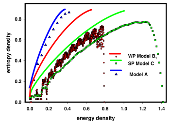
Figure 6: The canonical equivalence of the entropy $\overline{s}$ as a function of average energy $\overline{e}$ (continuous curves), and the microcanonical entropy (points) as a function of discreet energy $e$ for a given sequence $(M=24)$ for the three models. We consider unrestricted conformations here. The energy density has been shifted by the lowest energy density $e_{0}$ of each model so that the lowest shifted energy density is the same ($=0$) for all models. We notice a clear band band structure in $s$ in the perturbed models (B₁ and C₁). The bands become more pronounced and their separation also decreases, as $M$ increases (results not shown). We also see that the native state is almost disjoint from the rest of the bands. This is merely a reflection of the energy gap in the standard model A at low energies due to finite size of the protein.

VII.2.2 Convex Regions in $S(E)$

To understand the absence of concavity, we first consider the standard model A. The energy in this model is always negative, so there is no harm in considering the entropy as a function of the absolute energy $\left|E\right|=N_{\text{HH}}.$ In all cases that we have studied, $S(N_{\text{HH}})$ is found to be a concave discrete function. The number of states $W(N_{\text{HH}})$ can be partitioned into $W(N_{\text{HH}},\mathbf{N}^{\prime})$; see (20). In the model B, in which the energies are weakly perturbed, $\mathbf{e}^{\prime}\simeq 0;$ therefore, most of the conformations in $W(N_{\text{HH}})$ have energies that are close to $(-N_{\text{HH}});$ some of them will have energies that are outside the range ($-N_{\text{HH}}-1,-N_{\text{HH}}+1).$ The resulting $S(E)$ associated with this $N_{\text{HH}}$ is almost concave, as seen in each of the bands in Fig. 6; see the mathematical fits for the two of the bands blown up in Figs. 7, and 8 where the minibands within each of the bands are also evident. This then give rise to the lack of concavity or the emergence of convexity in the region where two nearby bands overlap. The number of bands equals the number of possible values of $N_{\text{HH}}$ in the model A. These convex portions of $s(e)$ should disappear and $s(e)$ should approach $\overline{s}(\overline{e})$ from below as $M\rightarrow\infty$   Guj0412548 . But for small systems, the convex regions persists. The band structure persists for all sequences that we have checked. The strongly perturbed energies in the model C provide enough spread for each band to strongly overlap, especially at the upper end of the energy spectrum, which reduces the size of convex regions. Even here, we find that the band nature survives at the upper end of the energies near the maximum; the bands at the lower end of the energy spectrum continue to persist even for strong perturbation. This is clear from Fig.(6). Thus, we are confident that convex regions in $S(E)$ will exist in any realistic model of small proteins. Their presence, however, does not imply any phase transition, as $\overline{S}(\overline{E})$ is always concave. This is true even though we note from Fig. 6, that there is a clear gap between the bands at the lowest energy; see also Fig. 22 for a clear evidence of such a gap near the native state where we have shown the entropy density for the model B₁ for low energies. The presence of bands alone and not the energy gaps between them give rise to convexity in $S(E),$ but not in $\overline{S}(\overline{E}).$ One does not need any energy gap for a convex $S(E)$ as was the case for the random energy model. The energy gaps between the bands in the present case are due to the discreteness inherent in small systems. As the bands disappear in $s(e)$ in the $M\rightarrow\infty$ limit, there will be no energy gap in this limit, as discussed earlier in Sect. III.4.

VII.3 Behavior of $S(E)$ in its bands

Let us now investigate the behavior of $s(e)$ in these bands by finding some smooth fits by neglecting its oscillatory pattern. We consider the two top most bands for the weakly perturbed model B₁, which are reproduced in Figs. 7 and 8, respectively, along with the best quadratic and cubic fits and their R values. It should be noted that the quadratic fit is equivalent to the Gaussian form (6), provided the coefficient of the quadratic term is negative. Because of the nature of each of these bands, this is true. If the linear term is positive (negative), then the most probable energy $\widetilde{E}_{\text{b}}$ within the band is positive (negative). From Fig. 7, we observe that the Gaussian fit is extremely poor in comparison with the cubit fit; even the latter fit is not too good. On the other hand, the result for the next band in Fig. 8 shows that both fits are similar in their R-values and that both are poor. This is because of the oscillating nature of $s(e)$ in the bands. It is interesting to note that the cubic fit is better for the top most band than the next lower one. But this cubic fit is not a concave function.

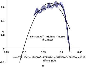
Figure 7: Entropy fit for the last band for the model B${}_{1\text{ }}$with $M=22$ and unrestricted conformations.

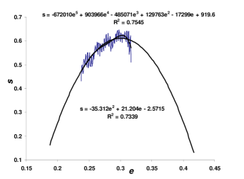
Figure 8: Entropy fit for the next to the last band for the model B${}_{1\text{ }}$with $M=22$ and unrestricted conformations.

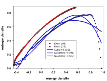
Figure 9: Exact ME and CE entropy density for the SP model C₁ (unrestricted conformations) along with quadratic and cubic fits.

VII.4 Numerical Fits for $S(E)$ and $\overline{S}(\overline{E})$

In Fig. 9 we reproduce the ME and CE entropy density for the strongly perturbed C₁ model (unrestricted conformations); we also show the best quadratic and cubic fits along their R values. The fits for the ME entropy are

$$s =0.3852+0.9875e+0.1136e^{2}-1.182e^{3}\ \ (R=0.9594),$$

$$s =0.4592+0.8717e-0.8221e^{2}\ \ (R=0.9197).$$

It is clear that between the two, the cubic fit is the better fit overall. However, both fits are extremely poor at the low energy end, which is the relevant range for the folded or the native state. Thus, the quadratic fit, which as said above is the Gaussian form (6), is not suitable to describe the ME entropy. Moreover, the quadratic fit gives rise to the vanishing of the entropy at an energy higher than the lowest allowed energy $e_{0}$, which is most certainly not true of the exact entropy, which is everywhere non-negative ($e\geq e_{0}$). It is not possible for the entropy to vanish at the lower end of the energy as $M\rightarrow\infty$, as there is not an energy gap in our model; see Sect. III.4. Hence, to conclude an ideal glass transition based on the vanishing of the Gaussian fit of the ME entropy is misleading even for small proteins. Even the prediction of an energy gap is misleading as there are several energy levels between the energy $E_{\text{F}}$ and $E_{0}.$ The presence of a convex region in the entropy $s\left(e\right)$ in both fits has nothing to do with any phase transition as the canonical entropy does not show any signature of a transition, as is clear from the figure.

The fits for the CE entropy are given by

$$\overline{s} =0.8236+0.9162\overline{e}-2.6895\overline{e}^{2}-0.27950\overline{e}^{3}\ (R=0.9843),$$

$$\overline{s} =0.5711+0.8511\overline{e}-0.5434\overline{e}^{2}\ (R=0.9994).$$

For the CE case, the quadratic fit is the better one; however, both fail in the low energy range. Thus, these fits also do not do justice to the native state. It should be noted, however, that both fits yield a positive CE entropy at all energies $e\geq e_{0}$.

In Fig.(10), we show the entropies and their best quadratic and cubic fits for the weakly perturbed model B₁. For the ME case, we have

$$s =0.4341+1.1203e-0.8863e^{2}-1.9502e^{3}\ (R=0.9663),$$

$$s =0.4406+0.9705e-1.1454e^{2}\ (R=0.9623).$$

Again, both fits are poor at the lower energy range; otherwise, they are very similar in their R-values. The Gaussian fit again predicts an energy gap, just as was the case for the strongly perturbed model in Fig.9, and has no significance for any folding transition. The exact discrete entropy $s(e)$ does show an energy gap between the two lower bands, which is expected to disappear in the limit $M\rightarrow\infty$. The prediction of negative ME entropy from the Gaussian fit is unphysical as above for the same reason, and cannot be taken seriously.

For the CE, the fits are:

$$\overline{s} =0.7029+0.9772\overline{e}-1.2906\overline{e}^{2}-0.8344\overline{e}^{3}\ (R=0.9995),$$

$$\overline{s} =0.7020+1.0448\overline{e}-1.3558\overline{e}^{2}\ (R=0.9994).$$

The behavior of the two fits are similar to that for the strongly perturbed case above. Once again, the ME entropy fits give non-negative entropy for all energies $e\geq e_{0}$.

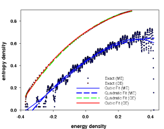
Figure 10: Exact ME and CE entropy density for the WP model B₁ (unrestricted conformations) along with quadratic and cubic fits.

VIII Energetics Effects on Densities and Specific Heat

VIII.1 Densities and Energetics

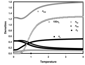
Figure 11: Densities for $M=16$ with only H residues (unrestricted conformations). The energetics belong to the strongly perturnbed case, with only $e_{\text{b}}=1,$ but all other elements in $\mathbf{e}^{\prime}$ are zero.

To understand the effect of bending only due to semiflexibility, we consider an unrestricted protein with $M=16$ that belongs to the strongly perturbed case; see Fig. 11. The only non-zero energies are $e_{\text{b}}=1,$ and $e_{\text{HH}}=-1.$ All other energies in $\mathbf{e}^{\prime}$ are zero. Thus, we are considering the model C${}_{2}.$ Furthermore, all residues are H; there is no P residue. This means that $n_{\text{PP}}=n_{\text{PW}}=0$ at all temperatures. There is a unique native state in which the protein bends around in a double strand

RRRRRRRDLLLLLLL

with $N_{\text{b}}=2,$ and $N_{\text{HH}}=7$ so that it has the energy $E=-5$. Other quantities of interest are: $N_{\text{p}}=7,N_{\text{hp}}=1,N_{\text{h}}=0,N_{\text{HW}}=20,$ and $N_{\text{PH}}=0.$ The fact that the entire protein is exposed to the water is understandable, as there is no interaction with water in this case. This is the state of the protein at $T=0.$ As $T$ is raised, the various densities behave as shown in Fig. 11. It is not surprising that $n_{\text{HH}}$ mostly decreases monotonically due to the penetration of water inside the protein.

What one notices from the figure is that around $T\simeq 0.5,$ there is not only a sudden rise in the helix density, a sudden drop in the parallel bond pair and HH-contact densities, but also a minimum in the HW-contact density. This minimum is due to the bending penalty as we now discuss. As said above, the native state corresponds to a double strand $(N_{\text{HH}}=7,$ and $N_{\text{HW}}=20).$ This state does not have the maximum HH-contact, which happens in a compact state ($N_{\text{HH}}=9$). However, the compact state corresponds to at least $4$ additional bends ($N_{\text{b}}=6$), so its energy is at least $E=-3,$ and is higher relative to the native state. At higher temperatures, the compact state, which has higher entropy, becomes more stable. This heuristically justifies the dip in $n_{\text{HW}}.$ While it is not noticeable in the figure, $n_{\text{HH}}$ has a maximum ($=0.4539$) at $T=0.42,$ exactly where the dip is in $n_{\text{HW}}$ ($=1.2172$ at $T=0.42$).

To understand the effects of the energetics better, we now give the results for a $M=24$ protein with a fixed sequence $\chi_{0}$. We consider the weakly perturbed model B${}_{1}.$ As said above, there are two native states related by the symmetry transformation (30). In the native state, we have $\mathbf{N}=(18,12,9,7,10,4,0),$ and $E=-446/50.$ The results for the densities as a function of $T$ are presented in Fig. 12. We observe that the rate of $n_{\text{PH}}$ rise is maximum around $T=0.58;$ in the neighborhood of this temperature, almost all densities in Fig. 12 have some unusual behavior. For example, $n_{\text{HH}}$ has a rapid drop around this temperature. Other densities seem to have a plateau around this temperature. As a matter of fact, all densities have an inflection point around this temperature.

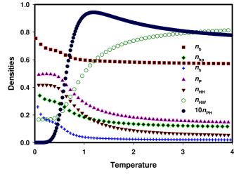
Figure 12: Densities for $M=24$ protein (unrestricted conformations). The energetics belong to the weakly perturnbed case. The sequence is prseset to the repeatation of PHHP.

VIII.2 Shifted Energy, Excitations, and Energetics

An interesting property of the three models should be noted from the above Fig.(6). The three entropies $\overline{s}(\overline{e})$ are drawn in such a way that the upper end of each of them corresponds to $T=4.0.$ What we see is that the corresponding shifted energies in the three models satisfy the following inequality:

$$\overline{E}_{\text{C}}(4.0)-\overline{E}_{\text{C}}(0)>\overline{E}_{\text{B}}(4.0)-\overline{E}_{\text{B}}(0)>\overline{E}_{\text{A}}(4.0)-\overline{E}_{\text{A}}(0).$$ (62)

Thus, at high temperatures, the excess energy above the native state of a given model is highest for the strongly perturbed model and lowest for the unperturbed model. This should not be taken as to mean that the heat capacity of the strongly perturbed model is the highest. We will return to this issue later.

We see from (62) that the excess energy of the strongly perturbed model is the highest at $T=4.$ In Fig. 13, we report the exact excess energies $\overline{E}(T)-\overline{E}(0)$ for the three models, A, B${}_{1},$ and C₁ $(M=24)$ on an infinite lattice. We see that the behavior changes at low temperatures, where the inequality of (62) is completely reversed. In other words, there are more excitations in the unperturbed model than in the perturbed models. This means that the net effect of the perturbations is to make the native state more robust to perturbations: The perturbations stabilize the native state to higher temperatures.

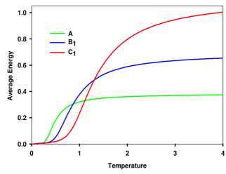
Figure 13: Shifted average energies for the three models for $M=24$ (unrestricted conformations).

VIII.3 Energy Fluctuations or Specific Heat

We report the energy fluctuations in Fig. 14 for the three models (unrestricted $M=24$ protein). The fluctuation is related to the specific heat in the model; see (47). The peaks in these fluctuations suggest strong fluctuations due to cooperativity in the models and are located at the inflection points in the average energies. As is known, these peaks usually provide a clue to an impending thermodynamically sharp transition in the thermodynamic limit. To understand such a claim better, we also report in the same figure the energy fluctuation for the unrestricted protein ($M=22)$ in model A. The peak of this fluctuation is somewhat lower in height than the corresponding peak for $M=24,$ thus suggesting that the peak height has increased with the protein size $M$. Standard statistical mechanical arguments require the energy fluctuations in the energy density to decrease with the size $M$ for macroscopic systems as follows:

$$\overline{(\Delta e)^{2}}\propto 1/M.$$

Thus, the fluctuations behave differently for small systems. The increase, however, is not very much, suggesting that the peaks may not diverge as will be the case for a continuous folding transition. We expect the folding transition to be a discontinuous one in the thermodynamic limit. However, more work is needed to settle this point.

The locations of the peak for the weakly perturbed model is at higher temperatures than the temperatures around $T=0.58,$ where the densities show unusual behavior. This is most probably due to the finite size effects, and should not be surprising.

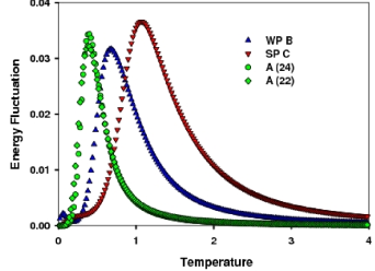
Figure 14: Energy fluctuations $\overline{(\Delta e)^{2}}$ for the three models for $M=24$ (unrestricted conformations). For comparision,we also show the fluctuation in the standard model for $M=22.$ We clearly see that the fluctuations become stronger as $M$ increases, but the postion of the peak does not shift much.

IX Conformational Space and Distance

IX.1 Distance Matrix

IX.1.1 Conformations or Microstates and Configurational Space $\mathbb{C}$

For monomeric systems, in which each monomer is treated as a particle, the energy landscape is easy to characterize. One labels the monomers $\alpha(=1,2,...,M)$ so that each monomer has a unique index $\alpha$. Then one considers their positions $\mathbf{r}^{(\alpha)}.$ The ordered set

$$\mathbf{R\equiv}\left\{\mathbf{r}^{(1)},\mathbf{r}^{(2)},\mathbf{r}^{(3)},...,\mathbf{r}^{(M)}\right\}$$

specifies a point in the $3M$-dimensional configuration space $\mathbb{C}$, and the energy $E$ associated with this configuration then defines the energy landscape in a $(3M+1)$-dimensional hyperspace. As only the ordered set $\mathbf{R}$ is used, permutation of particles positions is not allowed. Thus, each point in the configuration space represents a distinct microstate of the system. The ordered nature of the set $\mathbf{R}$ also takes into account for the connectivity of the protein: a residue occupying the lattice site $\mathbf{r}^{(k)}$ is connected to its neighboring residues located at lattice sites $\mathbf{r}^{(k-1)}$ (for $k>1$) and $\mathbf{r}^{(k+1)}$ (for $k<M$). To see this most easily, we proceed as follows. We take the C-terminus of the protein to be the starting point of the sequence. We index the starting point as the first residue, which is used to root the protein. Each successive residue in the sequence is, hereafter, given an index increasing by one, until the last residue is given the index $M$. The location of a site on the lattice is also given by a doublet $\mathbf{r}=(x,y)$ with the location of the root given by the doublet $(0,0).$ Because of the choice of the lattice spacing ($a=1$), the coordinates $x,y$ are integers. The conformation of the protein is uniquely given by the ordered sequence of the doublets $\mathbf{R\equiv}\left\{\mathbf{r}^{(\alpha)}\right\},$ where the residue $\alpha(=1,2,...,M)$ is located at the lattice site $\mathbf{r}^{(\alpha)}.$ We also require the first bond of the protein to be in a fixed direction. Each ordered sequence $\mathbf{R}$ specifies a protein conformation, a microstate, $\mathbf{\Gamma}$ uniquely. There are altogether $W$ distinct conformations or microstates. In the following, we will also use state to simply refer to a microstate or a conformation.

IX.1.2 Distance between Conformations

The distance between two conformations $\mathbf{R}$ and $\mathbf{R}^{\prime}\mathbf{\equiv}\left\{\mathbf{r}^{\prime(\alpha)}\right\}$ is defined here to be the Euclidean distance

$$d(\mathbf{R},\mathbf{R}^{\prime})=\sqrt{\sum\limits_{\alpha=1}^{M}[\mathbf{r}^{(\alpha)}-\mathbf{r}^{\prime(\alpha)}]^{2}.}$$

The distance provides useful information not only about the topology of the energy landscape but may also be relevant for the dynamical description of the folding process (even though we are not presently interested in the dynamics) by introducing the concept of a neighborhood of a point in the conformation space $\mathbb{C}$: two conformations are neighbors or are connected in $\mathbb{C}$ if their separation is less than or equal to some chosen distance.

IX.1.3 Distance or Neighborhood Matrix

The distance $d(\mathbf{R},\mathbf{R}^{\prime})$ can be used as an element to define a $W\times W$ distance or neighborhood matrix $\mathcal{D}\mathbf{,}$ whose diagonal elements are the only elements that are $0\mathbf{.}$ All other elements are non-zero. Thus, $\mathcal{D}$ is not going to be a sparse matrix. The distance between a compact conformation and a completely extended conformation will be among the largest. The shortest distances will usually be between two conformations that differ in a few elements. For example, assume that only the elements $\mathbf{r}^{(M)}$ and $\mathbf{r}^{\prime(M)}$ differ. The two elements can only differ in one of its components, and that too by only one lattice spacing. Thus, the distance between these two conformations will be $1.$ It is also possible that two conformations differ in only one interior element at the position $k\neq M.$ The vectors $\mathbf{r}^{(k)}$ and $\mathbf{r}^{\prime(k)}$ must differ in each of their components by $1.$ Hence, the distance between these conformations will be $\sqrt{2}.$

IX.1.4 Native (0) and Stretched (S) States

As $W$ is usually a large number, it is not possible to study the entire matrix $\mathcal{D}$. Therefore, we will consider the distance of each conformation from two selective conformations, viz. the native state (to be denoted by 0 in the following) and the completely stretched state (to be denoted by S in the following); the latter is the conformation in which the protein is given by the string of only R steps

$$\text{{\normalsize RRR...}}{\normalsize.\ }$$

so that the conformation is completely in the horizontal direction. If the native state is not unique, we pick the first one of the generated native states. The stretched conformation is unique in that it does not depend on the energetics. On the other hand, the native conformation depends strongly on the energetics and, therefore, is not unique as far as different energetics are concerned. This feature makes the stretched conformation a desirable reference state. This state can be used to compare proteins with different energetics. We denote the two distances by $d_{\text{0}}(\mathbf{R})$ (from the native conformation) and $d_{\text{S}}(\mathbf{R})$ (from the stretched conformation), respectively. In most cases of interest, there is a unique native state for a given energetics. It is the standard model which invariably gives rise to degenerate native states.

Let the set $\mathbf{R}_{l}\mathbf{\equiv}\left\{\mathbf{r}_{l}^{(\alpha)}\right\}$ denote the two reference conformations $\left(l=\text{0,S}\right)$, and

$$d_{l}(\mathbf{R})=\sqrt{\sum\limits_{\alpha=1}^{M}[\mathbf{r}^{(\alpha)}-\mathbf{r}_{l}^{(\alpha)}]^{2}}$$

the distance of some conformation $\Gamma$ specified by the set $\mathbf{R}$ from $\mathbf{R}_{l}$. This distance of a conformation of energy $E(\mathbf{R})$ gives information about how close that conformation is to the native state. Thus, we can classify each conformation by its distance $d_{l}$ and energy $E$ and present them in a two-dimensional plot as in Figs. 15,16,17,18,20,19 and 21. In all these plots, we have shifted the energy so that the native state energy is at $0,$ so that we can compare the configuration space $\mathbb{C}$ of proteins with different energetics. Moreover, we only consider one of the native states if there are several native states to save computational time. In this sense, our results are not complete in such cases. Therefore, we also present the result for a weakly interacting $M=16$ protein of a sequence for which there exists only one unique native state so that we can compare this complete case with the incomplete case. We will find that there is no dramatic difference.

IX.1.5 Reduction of $\mathbb{C}$ to a 2-dimensional plane $\mathbb{C}_{2l}$

The use of the two reference states will provide us with two distinct but partial perspectives of the configuration space $\mathbb{C}$ by projecting it on a lower dimensional space. Let us consider the perspective of $\mathbb{C}$ while looking at it from the native state. The projected plane is denoted by $\mathbb{C}_{2\text{0}}.$Imagine the energy distribution of conformations that are a distance $d_{\text{0}}$ from the native state. All these states are on a hypersphere of radius $d_{\text{0}}$ and have various energies. Let us further coalesce all of the conformations of a given energy $E$ that lie on this hypersphere to a single point. We will use $W(d_{\text{0}},e)$ to represent the number of these conformations associated with the single point in $\mathbb{C}_{2\text{0}}$. Such a transformation allows us to transform $\mathbb{C}$ to a two-dimensional surface $\mathbb{C}_{2\text{0}}$ on which a point is represented by ($d_{\text{0}},e$). On such a plane, a constant energy line represents the equipotential conformations at various distances from the native state. All these conformations are at the same height (from the native state) in the energy landscape. A constant $d_{\text{0}}$ line represents all conformation with various energies that lie on a hypersphere centered at the native state. A similar reduction from $\mathbb{C}$ to the two-dimensional surface ($d_{\text{S}},e$) provides another perspective of the energy landscape. We will use $W(d_{\text{S}},e)$ to represent the number of conformations associated with the single point in the above coalescing on the ($d_{\text{S}},e$) plane. The projected plane is denoted by $\mathbb{C}_{2\text{S}}.$

It is obvious that

$$W(e)\equiv\sum_{d_{l}}W(d_{l},e),\text{ }l=\text{0,S,}$$ (63)

so that the two perspectives only differ in the way $W(e)$ is partitioned into $W(d_{l},e)$ by the distance $d_{l}$. The total number of microstates $W(e)$ remains the same in the two perspectives. In addition, the allowed energies also do not change in the two representations of $\mathbb{C}.$

IX.2 Standard Model

The first two figures, Figs. 15 and Fig. 16 are for the standard model. Fig. 15 shows the energy density distribution vs. $d_{\text{0}}$ (red circles: $\mathbb{C}_{2\text{0}}$) or $d_{\text{S}}$ (blue triangles: $\mathbb{C}_{2\text{S}}$), respectively; they are two possible perspectives of $\mathbb{C}$. The two conformations at $d=0$ in Fig. 15 represents the native conformation (red circle at $e=0$) and the extended state (blue triangle at $e=3/8$) that are used as the origin of the distance for the two perspectives, respectively. We observe that both the maximum and the minimum $d_{\text{0}}$ increase with $e,$ the former more so than the latter. However, while the maximum $d_{\text{S}}$ increases with $e,$ the minimum $d_{\text{S}}$ decrease with $e.$ We observe that the maximum $d_{\text{0}},$ to be denoted by $d_{\text{0,max}},$ is about 120, while the maximum $d_{\text{S}},$ to be denoted by $d_{\text{S,max}},$ is about 200. As said above, the number of conformations $W(e)$ for a given energy, and the allowed energies ($7$ in total) are the same for both distributions. The left axis shows $e$ for the red circles and the left axis for the blue triangles. The left axis has been shifted by $0.02$ so that the two colors do not overlap. In Fig. 16, we show the $3$-d plot $d-e-W(d,e)$ as the projected energy landscape built on $\mathbb{C}_{2\text{0}}$ (red circles) and $\mathbb{C}_{2\text{S}}$ (blue triangles). The energies for blue triangles has been shifted by 0.02 so that the two symbols will not overlap. We observe that for a given $e$, $W(d,e)$ has a single peak in $\mathbb{C}_{2\text{0}}$ (red circles), while it has several peaks in $\mathbb{C}_{2\text{S}}$ (blue triangles). Moreover, the peaks in $\mathbb{C}_{2\text{0}}$ rise and move away from the native state as we approach higher energies.

Because of the sum rule (63) and the fact that the allowed $d$-range of $d_{\text{S}}$ is much larger than of $d_{\text{0}},$ it is not surprising that $W(d_{\text{0}},e)$ is much higher near its peak than $W(d_{\text{S}},e)$ near its peaks. It is clear that many high energy conformations are far from the extended conformation of the same high energy, but most of these high energy conformations are closer in distance from the native conformation. This suggests a very open landscape for the standard model with the native state in the middle, and which continues to narrow down with decreasing energy. We also note that $\mathbb{C}_{2\text{S}}$ is more symmetric than $\mathbb{C}_{2\text{0}}$. We also observe that the native state is around $d_{\text{S}}\simeq 90$ from the stretched state ($e=3/8$); see blue triangles. It follows from the figures that there are several other states of energy $e=7/16$ that are much closer to the native state. Indeed, there are high energy states as close as about $d_{\text{0}}=10.$

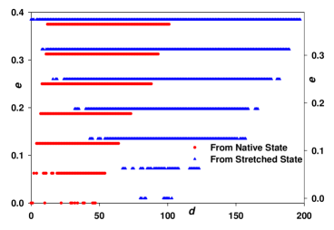
Figure 15: $E$ vs. $d_{\text{S}}$ distribution for for $M=16$ Model A protein (unrestricted conformations).

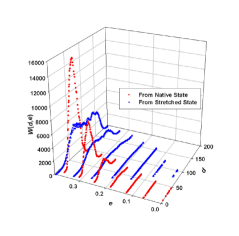
Figure 16: $E$ vs. $d_{\text{0}}$ distribution for $M=16$ Model A protein (unrestricted conformations).

We comment on some interesting features that is apparent in the figures. Consider Fig. 15. The best way to understand this figure is to imagine drawing a (hyper)circle of radius $d$ with its center at the chosen native state. Now draw a (hyper)cylinder on this circle along the energy direction. Then the microstates that lie on this cylinder are the microstates (red circles) that appear on the vertical line drawn at the distance $d$ (from the native state) in Fig. 15. All of these microstates are on the cylinder of radius $d,$ but the distances between them may be much different from $d$. In fact, some of them may be closer than $d,$ while others may be farther apart.

The conformation closest to the native state in Fig. 15 is not at $e=1/16,$ but another native state. Thus, there is no energy barrier between these two microstates (at the same energy). However, there are other microstates at the lowest energy that are widely separated in the radial direction of $d_{0}.$ The same is true of states at $e=1/16$. (At higher energies, the microstates are almost dense in $d_{0},$ so that can be treated as connected in that they lie on neighboring cylinders.) Consider the microstates at $e=1/16.$ Between various separations (in the direction of $d_{0}$) in these states exist many higher energy states at $e=2/16$. This is true in other figures also. Thus, this feature appears to be generic. But this is true only of the lowest lying microstates. The microstates at higher energies are connected in the sense note above. Thus, the energy barriers in the radial direction exist only for low-lying states. There are no barriers in the radial direction for highly excited states. This does not imply that there are no barriers in other transverse directions in the configurations space $\mathbb{C}.$ The implication of this for the possible dynamics can be easily appreciated if we recognize that only local moves are possible in a suitably chosen short duration $\tau$. During this time $\tau$, the protein can only change its conformation to a new conformation that is nearby in distance. Thus, in the process of folding, the protein will more efficiently move to the native state from $e=2/16$ than from $e=1/16,$ if the former is closer to the native state than the latter. We will not pursue this point further here as we are only considering equilibrium properties in this work. We hope to return to this issue in a future contribution.

IX.3 Weakly Perturbed Model

The energy density $e$ in the standard model changes by a non-zero but appreciable amount $\Delta e=1/16.$ This can be made smaller by introducing other energies in the model. For the model B₂, the results are shown in Figs. (17, and 18) for the sequence $\chi_{0}$. In Fig. 17, we show $\mathbb{C}_{2\text{0}}$ along with the distribution $W(d_{\text{0}},e)$ for some selected distances $d_{\text{0}}=20,30,40,50,$ and $60.$ In Fig. 18, we show $\mathbb{C}_{2\text{S}}.$ The discrete band structure of Figs. (15, and 16) still persists even to the higher energies, except that $\Delta e$ is smaller, and the energy spectrum begins to look more continuous at higher energies. At energies close to the native state, the spectrum is still very much discrete. Otherwise, the features of the model A have not disappeared. For example, the symmetry in $\mathbb{C}_{2\text{S}}$ is still present; see Figs. (16, and 18). In Fig. 19, we show the result for a weakly interacting Model B₂ $M=16$ unrestricted protein for the following sequence:

$$\chi:\text{ PPPPHHPPHHHHHHHPP.}$$

In this case, there is only one unique native state, which is given by the string

RRRDDDLUULDLULD

starting with the first residue. The energy of the native state has $\mathbf{N}=(9,6,4,2,4,4,4),$ and $E_{0}=-117/56.$ However, a comparison with Fig. 18 shows that the distributions of states in $\mathbb{C}_{2\text{S}}$ for the two cases are almost the same, except at low energies. Thus, we believe that our incomplete results are not different from the complete results at intermediate and higher energies.

The distribution $W(d_{\text{0}},e)$ in Fig. 17 shows that it has an oscillatory pattern and that the highest peak in it has a maximum around $d_{\text{0}}=60,$ and $e=0.7.$

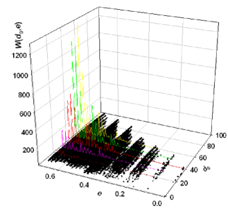
Figure 17: $E$ vs. $d_{\text{0}}$ distribution for for $M=16$ Model B₂ protein (unrestricted conformations).

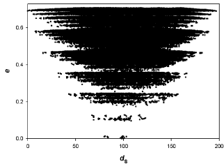
Figure 18: $E$ vs. $d_{\text{S}}$ distribution for $M=16$ Model B₂ protein (unrestricted conformations) for the sequence $\chi_{0}$.

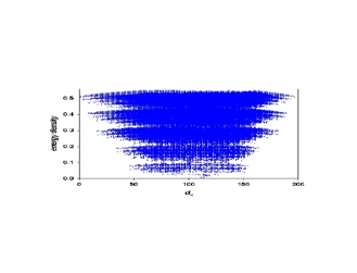
Figure 19: $E$ vs. $d_{\text{S}}$ distribution for $M=16$ Model B₂ protein (unrestricted conformations) for the sequence $\chi:$ PPPPHHPPHHHHHHHPP.

IX.4 Strongly Perturbed Model

The projected conformation spaces $\mathbb{C}_{2\text{0}}$ and $\mathbb{C}_{2\text{S}}$ for model C₁ are shown in Figs. 20 and 21, respectively. We again see the symmetry present in the distribution of states in $\mathbb{C}_{2\text{S}}.$ The energetics is such that there is a strong mixing of levels to the point that the clear cut band pattern is completely absent at high energies; their discrete nature is still present near the bottom. The energetics change the native state so that its distance from the extended state are different in the three models.

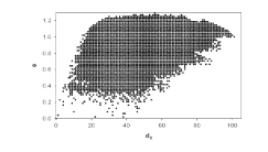
Figure 20: $E$ vs. $d_{\text{0}}$ distribution for $M=16$ Model C₁ protein (unrestricted conformations).

Figure 21: $E$ vs. $d_{\text{S}}$ distribution for $M=16$ Model C₁ protein (unrestricted conformations).

IX.5 Small System Energy Landscape and Convexity of $S(E)$

The distribution of points in the $\mathbb{C}_{2}$ plane allows us to draw certain conclusions about the form of the energy landscape. Assume that the energy landscape is a single inverted cone of a fixed (hyper-solid)angle. In that case, all conformations of a given energy $E$ will have the same radial distance from the native state in $\mathbb{C}$, and the energy-distance distribution in $\mathbb{C}_{2\text{0}}$ will be represented by points that lie along a single straight line at a fixed angle in the $e-d_{0}$ plane: For each energy, all states are collapsed into a single point on this line. This is most obviously not the case here in any of the $\mathbb{C}_{2\text{0}}$ for the three models shown here. Consider the standard model in Fig.(15). We see that there are a few allowed energies at a given distance $d_{\text{0}}$ from the native state. If we draw a hypercylinder of radius $d_{\text{0}},$ then this cylinder will cut the landscape at these energies. These energies are at different angles so they lie on different cones making different angles at its apex located at the native state. The number of points the hypercylinder cuts the landscape is given by the sum

$$W(d_{0})\equiv\sum_{E}W(d_{0},E),$$

where $W(d_{0},E)$ is the number of conformations of energy $E$ that are at the radial distance $d_{0}$ from the native state.

Because of conformational changes during folding, the folding is believed to be governed by the multiplicity $W(E),$ which in turn governs the energy landscape Guj0412548 : each point on the hypersurface represents a conformation. The lack of concavity discovered here has a profound effect on the shape of the landscape. It no longer narrows down as $E$ decreases. It will be interesting to pursue this point further. This is beyond the scope of the present work, but we hope to consider it elsewhere. It is evident, and as discussed above, several different $\mathbf{N}$ will usually mix together for a given $E$, except in the model (A) [in which $E=-N_{\text{HH}}$]. There will be a certain landscape topology for the standard model, which will change with $\mathbf{e}^{\prime}$. From (20), it is evident that the landscape will become narrower for $\mathbf{e}^{\prime}\neq 0.$ At the same time, the total ”surface area” $W$ of the landscape will not change (even though the allowed energies change) with $\mathbf{e}^{\prime}.$ It is possible that it is this narrowing at constant $W$ that makes the approach to native state more directional with the consequence that it would be fast. This issue needs to be probed carefully.

Since it is CE that is relevant for a real protein in its environment, it is the canonical multiplicity

$$W_{\text{CE}}(\overline{E})\equiv\exp[\overline{S}(\overline{E})]$$

that is relevant for folding. As shown above in (61), it continuously increases with $\overline{E},$ until we reach at infinite temperatures. Thus, the narrowing of the landscape with non-zero $\mathbf{e}^{\prime}$ may not be as relevant for protein folding as the observation that $W_{\text{CE}}(\overline{E})>W(\overline{E}).$ From (58), we observe that $W_{\text{CE}}(\overline{E})$ gets contribution from all conformations, not just the conformations $W$ associated with $\overline{E}.$ In particular, it also includes the contribution from the native state(s) though its probability is going to be small unless we are at very low temperatures. Thus, it is misleading to think that a small protein at a given $T$ only probes average conformations $W(\overline{E})$ when in equilibrium. As $T$ is reduced, the protein continues to probe all conformations although the probability for conformations of lower energies increases. It would be interesting to pursue the consequence(s) of this observation.

X Free Energy Landscape and $\partial S(E)/\partial E$

X.1 Free Energy Landscape

Let us consider the implications of the non-concavity of $S(E)$ on the free energy functional

$$F(E,T)\equiv E-TS(E),$$

which should not be confused with $F(T)$ introduced earlier in (50) and (51). The later represents the free energy of the equilibrium state of the system. It is a monotonic function of $T$, and because $\overline{E}$ is monotonic in $T,$ it is also a monotonic function of $\overline{E}.$ On the other hand, the functional $F(E,T)$ is defined at any $T$ as a function of $E$. Thus, it is also defined for energies different from the equilibrium energy at $T$. For a macroscopic system, it is well known that one must minimize globally $F(E,T)$ with respect to $E$ at fixed $\ T$ to obtain the equilibrium free energy $F(T)=F(\overline{E},T)$ evaluated at the minimum. For continuous functions, this minimization is equivalent to (61) for $S(E):$

$$\partial S(E)/\partial E=1/T.$$ (64)

Figure 22: The free energy functional $f(e,T)\equiv F(E,T)/M$ at three different temperatures $T=0.9,1.0,$ and $1.1$ for the model B${}_{1}.$ We also show the entropy $s(e)$ for low energies. The free energy functional describe the free energy landscape at a given temperature $T.$ The functions are discrete and the curves are drawn through their points only as a guide for the eye and to clearly show the undulations in them.

It is this relation (64) that was used for the Gaussian entropy (6) to obtain the Gaussian energy relation (8) earlier. The above discussion makes it clear that the derivation given there was valid for a macroscopic system, and not for a small system.

At a given temperature, the free energy functional $F(E,T)$ describes, what is customarily called the free energy landscape at that temperature with the energy $E$ playing the role of a reaction coordinate of the landscape. We show in Fig. 22 this landscape at three different temperatures $T=0.9,1.0,$ and $1.1$ for the weakly perturbed model B₁ $($unrestricted protein with $M=24).$ We have also shown the entropy density at low energies, which is a blow up of the entropy shown in Fig. 6.

X.2 Lack of Physical Significance of Global Minimum of $F(E,T)$

The global minima of the three landscapes occur at $e=-0.0783,-0.3717,$ and $0.0742,$ respectively. ($e_{0}=-0.3717.$) The depths of the minima are, respectively, $f=-0.4410,0,-0.4006,$ and $-0.5309.$ That the energy of the global minima and their depths as a function of temperature have no thermodynamic significance is obvious when we recognize that these energies and free energies are not monotonic in $T,$ whereas proper thermodynamics requires them to be monotonic even for small systems. It is interesting to compare these energies and the depth of the free energy minima with the exactly computed average energy density $\overline{e}(T)$ and the free energy $f(T).$ The computed average energies at these temperatures are $-0.0479,0.0054,$ and $0.0493,$ while the free energy densities are $-0.6294,-0.697,$ and $-0.7694.$

What is striking is the tremendous error in the computed values and those obtained by the application of macroscopic thermodynamic principle to small proteins. Neither the location nor their depth are close to the exact computed values. This is a sobering realization of the effects of the finite size of the protein on thermodynamics.

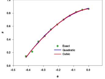
Figure 23: A quadratic and cubic fit for the ME entropy for $M=24$ Model A.

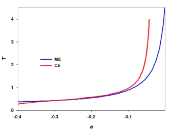
Figure 24: Calculation of $T$ using (64) for the cubic fit of the ME entropy in Fig.(23) and by using the CE entropy.

X.3 Error in Using $\partial S(E)/\partial E=1/T$

We consider the unperturbed model A for an unrestricted protein ($M=24$), whose ME entropy density as a function of the energy density is reproduced again in Fig. 23. As it is a discrete function, we cannot calculate its derivative to see if (64) is valid for small systems. However, it is possible to find a continuous fit for $s(e).$ We have shown a quadratic and a cubic fit in Fig. 23 along with the $R$-values. They are respectively

$$s =0.8737+0.5484e-3.0151e^{2};~{}\ \ R=0.9987,\$$

$$s =0.8650+0.2145e-5.1161e^{2}-3.361e^{3};~{}\ R=0.9990,\$$

and can be used to calculate the inverse derivative $\partial E/\partial S,$ which is plotted in Fig. 24 as the blue curve, along with the inverse derivative $\partial\overline{E}/\partial\overline{S}$ as the red curve. Here, we have used the cubic fit for the calculation of $\partial S/\partial E$. The difference shows the error caused by using (64) to calculate the inverse temperature. The correct temperature is given by the red curve. We find that the correct temperature from CE is lower than the incorrect temperature from ME at lower energies, with their nature reversed at higher temperatures. In other cases, it is also possible to observe the opposite relation for the two ways of computing the temperature.

XI Discussion and Conclusions

We have considered a lattice model of a small protein as a semiflexible copolymer in its solvent environment. The copolymer is random due to possible forms of its residue sequence, but this randomness is considered frozen (quenched). The model presented here is an extension of the original model of semiflexible homopolymer due to Flory; this extended model has been investigated recently by us. However, the model requires a very important modification because of the heteropolymer nature of the protein. Here, we have restricted our investigation to an incompressible copolymer representation of the protein. Another novelty is to restrict the analysis to a single protein size of a finite size $M$. Our previous investigation has involved either an infinitely long polymer or an infinite number of finite polymers. Thus, studying small system effects on the statistical mechanics of the protein has been a central feature of this investigation.

Our aim is to study exactly the statistical mechanics of the general model. For this, we take the approach of exact enumeration in which we count exactly the number of conformations of the protein by anchoring one of its ends, the C-terminus, at the origin of the lattice. We consider a square lattice and use its lattice symmetry to generate only those conformations whose first step from the origin is in the horizontal direction. This reduces the number of conformations by $4$. We also allow the first bend only in the downward direction, but not in the upward direction to further reduce the number of conformations that we generate. We consider two different kinds of conformations for enumeration. We either consider only compact conformations or consider unrestricted (compact and non-compact) conformations, and generate all conformations under the above two restrictions due to lattice symmetry. For compact conformations, we have considered $M\leq 64,$ and for unrestricted conformations, we have considered $M\leq 26$ so that the enumeration can be done in a reasonable amount of time. As real protein interactions are not well-understood, we have considered three different model energetics to study the effects of energetics on protein thermodynamics. One of the models (Model A) is the standard model, while the other two are obtained by weak perturbation (Model B), and strong perturbation (Model C).

Using plausible arguments under some very mild assumptions, we show that these models have no energy gap for $M\rightarrow\infty$, even though there appears to be some gap in the case of small proteins. Indeed, an energy gap is not the only way a discontinuous folding transition can occur. The latter is known to occur even in the absence of an energy gap such as the Flory model of semiflexible homopolymer as shown recently by us. However, the presence of a gap endows the microcanonical ensemble (Boltzmann) entropy $S(E)$ with non-concavity. For a macroscopic system, such a non-concave entropy implies a discontinuous folding transition. Thus, it is the non-concavity that drives the discontinuous folding transition and not the energy gap. However, we demonstrate that it is the canonical ensemble equivalent entropy function $\overline{S}(\overline{E})$ that shares the concavity requirement for small or macroscopic systems; the canonical entropy $S(E)$ is not required by thermodynamics to be concave. Moreover, we prove that $\overline{S}(\overline{E})\geq$ $S(\overline{E}).$Our exact enumeration confirm these facts. We show that a Gaussian fit is not very good for exact entropies that we calculate, especially at low energies, the energies most relevant for the folding transition. The Gaussian fit invariably gives rise to negative entropies that are then avoided by advocating an energy gap. This is despite the fact that the exact enumeration never leads to a negative entropy. Thus, the usefulness of the random energy model for small proteins is highly questionable.

It is plausible that infinite random copolymers are self-averaging. As a consequence, all thermodynamic densities are the same for almost all sequences. However, we find that small proteins are far from being self-averaging. Therefore, as is commonly believed, the protein sequence is extremely relevant for its proper or desired functioning. In other words, we cannot overlook the importance protein sequences have in determining the native state. Also, as expected, various densities such as the entropy and energy densities retain a strong dependence on $M$; this dependence should not be neglected. While a small protein is not supposed to show a sharp folding transition, a signature of a rounded folding transition appears in the peak in the specific heat.

We introduce a notion of a distance between conformations and show how the multi-dimensional configuration space $\mathbb{C}$ can be mapped onto a two-dimensional configuration space $\mathbb{C}_{2l}$,$l=$0,S. These two-dimensional projections provide a glimpse of the form of $\mathbb{C},$ and from which we obtain some limited perspective of the energy landscape. We also calculate the free energy landscape by using the energy density as the coordinate. These free energy landscape appear very flat with undulations that are not very high.

We have also shown that applying thermodynamic relations that are valid for macroscopic systems to small system microcanonical entropy will cause errors in estimating thermodynamic properties, and should be avoided.

- (1) C. Anfinsen, Science 181, 223 (1973). C. Anfinsen and H. Scheraga, Adv. Protein Chem. 29, 205 (1975). Y.H. Taketomi and N. Gō, Int. J. Pept. Protein Res. 7, 445 (1975). S. Govindarajan and RA Goldstein, Proc. Natl. Acad. Sci. USA 95, 5545 (1998).
- (2) It should be noted that proteins are in their native states only in an intermediate temperature range and unfold outside this range. Thus, the native state of a protein is an intermediate phase and not a phase that remains intact as we approach absolute zero. In this work, we will avoid this complication and consider the native state to be a state that can occur all the way down to absolute zero. Thus, the entropy of the native state at absolute zero will be zero in accordance with the third law of thermodynamics. On the other hand, a completely flexible copolymer in general will not have a zero entropy even at absolute zero. This again shows that we need to incorporate semiflexibility in our protein medeling.
- (3) According to our definition, a single protein system is small if is finite, even if the volume is infinitely large. In this case, will converge to zero. If also diverges with (the limiting concentration ), we will refer to this system as macroscopic. A system with can be either small or macroscopic depending on whether remains finite or not as diverges. A bulk system will always refer to the case of many proteins, which we do not consider here. For a single protein of finite , it is clear that if one of the ends of the protein is rooted at the center of the volume , then one does not need to take the limit , as long as the interactions are short-ranged. Then the rooted protein will never feel the effects of the boundary of as long as is sufficiently large.
- (4) A. Finkelstein and O.B. Ptitsyn, Protein Physics (Academic Press, London, 2002).
- (5) M-H Hao and H.A. Scheraga, J. Chem. Phys. 100, 14540 (1996).
- (6) K.F. Lau and K.A. Dill, Macromolecules 22, 3986 (1989).
- (7) S. Miyazawa and R. Jernigan, Macromolecules 18, 534 (1985).
- (8) A. Kolinski, W. Galazka, and J. Skolnick, Proteins: Struct. Funct. Genet. 26, 271 (1996).
- (9) M-H Hao and H.A. Scheraga, J. Mol. Biol. 277, 973 (1988); J. Chem. Phys. 107, 8089 (1997); Struct. Biol. 9, 18 (1999).
- (10) E. Shakhnovich, Phys. Rev. Lett. 72, 3907 (1994).
- (11) J. Venkatraman, S.C. Shankaramma, and P. Balaram, Chem. Rev. 101, 3131-3152 (2001).
- (12) C. Clementi, H. Nymeyer and J.N. Onuchic, J. Mol. Biol. 298, 937 (2000).
- (13) The number of conformations depends on the size of the protein, the residence sequence the topology of the lattice, etc. In the rest of the paper, we will not show this dependence explicitly for the sake of notational economy, but should not be forgotten. As we will discuss later, by rooting or anchoring the protein, as we do in this work, we make independent of
- (14) Since is a number, it can only be a function of a dimensionless quantity. Indeed, the arguments of any dimensionless function must be dimensionless. For , this requires introducing an arbitrary energy scale so that becomes a pure number. Then, we can introduce as a function of this dimensionless energy However, following the tradition, in the rest of this work, we will continue to express various quantities as functions of variables that customarily have dimensions such as or (in the units of the Boltzmann constant), keeping in mind that they have been made dimensionless by dividing by
- (15) E.J. Janse van Rensburg, A. Rechnitzer, M.S. Causo, and S.G. Wittington, J. Phys. A 34, 6381 (2001).
- (16) J.D. Bryngelson, J.N. Onuchic, N.D. Socci, and P.G. Wolynes, Proteins,21, 167 (1995).
- (17) J. Chuang, A Yu. Grosberg, and M. Kardar, Phys. Rev. Lett. 87, 078104 (2001);cond-mat/0102065.
- (18) F. Semerianov and P.D. Gujrati, Phys. Rev. E72, 011102 (2005).
- (19) N. Gō and H. Taketomi, Proc. Natl. Acad. Sci., USA 75, 559 (1978).
- (20) J. Skolnick, Proc. Natl. Acad. Sci., USA 102, 2265 (2005).
- (21) P.D. Gujrati, cond-mat/0412548.
- (22) P.D. Gujrati, and B. Lambeth, cond-mat/0708.2253.
- (23) In the thermodynamic limit () of an infinitely large macroscopic system, does not exist mathematically as it will be usually infinitely large in magnitude, and one must consider its density . For a small system under investigation here, one can study either or as both remain bounded.
- (24) An extensive quantity is a thermodynamic quantity that increases asymptotically linearly with the size (in our case ) of the system. Thus, the energy is extensive, but is not.
- (25) M.A. Miller and D.J. Wales, J. Chem. Phys. 111, 6610 (1999).
- (26) D.J. Wales, Energy Landscape: With Applications to Clusters, Biomolecules and Glasses (Cambridge University Press, Cambridge, 2003).
- (27) A. Sali, E. Shakhnovich, and M. Karplus, Nature 369,248 (1994); J. Mol. Bio. 235,1614 (1994).
- (28) D.A. Lidar, D. Thirumalai, R. Elbert, and R.B. Gerber, cond-mat/9808202.
- (29) B. Derrida, Phys. Rev. B24, 238 (1981).
- (30) The graph of a concave function (discrete or continuous) is one in which the line connecting its values at any two points must never lie above the function at intermediate points.
- (31) It should be noted that the Gaussian distribution in (3) cannot be truly a realistic distribution as it violates the constraint However, this violation is usually interpreted to imply a folding transition in proteins because of the resulting non-concavity of the entropy, as discussed later in this section. It should also be noted that (3) cannot be valid for small energies, where since is supposed to be an integer, while in (3) is a continuous variable. This is a serious matter, as the distribution function at small energies are crucial in determining the behavior of the folded state.
- (32) J.F. Nagle, Math. Phys. 13, 62 (1969).
- (33) J.F. Nagle, P.D. Gujrati, and M. Goldstein, J. Phys. Chem. 88, 4599 (1984).
- (34) C. Clementi and S.S. Plotkin, Protein Science, 13, 1750 (2004).
- (35) P.D. Gujrati, cond-mat/0309143.
- (36) P.D. Gujrati, and A. Corsi, Phys. Rev. Lett. 87, 025701 (2001); P.D. Gujrati, S.S. Rane, and A. Corsi, Phys. Rev. E 67, 052501 (2003); A. Corsi and P.D. Gujrati, Phys. Rev. E 68, 031502 (2003); S.S. Rane and P.D. Gujrati, Macromolecules 38, 8734 (2005).
- (37) H.S. Chan and K.A. Dill, J. Chem. Phys. 95, 3775 (1991); H.S. Chan and K.A. Dill, J. Chem. Phys. 100, 39238 (1994); K.A. Dill, S. Bromberg, K. Yue, K.M. Fiebig, D.P. Yee, P.D. Thomas, and H.S. Chan, Protein Sci. 4, 561 (1995). K.A. Dill, Protein Sci. 8,1166 (1999).
- (38) A better choice for the fit would have been which is known to be an appropriate asymptotic behavior for large . We have not done that. Our simple fit gives the -value shown in Fig. (2).
- (39) P.D. Gujrati, J. Chem. Phy. 112, 4806 (2000).
- (40) P.D. Gujrati, Phys. Rev. E 51, 957 (1995).
- (41) P.J. Flory, J. Chem. Phys. 10, 51(1942).
- (42) P.D. Gujrati, J. Phys. A 13, L437 (1980); P.D. Gujrati and M. Goldstein, J. Chem. Phys. 74, 2596 (1981); P.D. Gujrati, J. Stat. Phys. 28, 241 (1982).
- (43) M. Mezard, G. Parisi, and M.A. Virasoro, Spin Glass Theory and Beyond (World Scientific, Singapore, 1987).