Joint deprojection of Sunyaev–Zeldovich and X–ray images of galaxy clusters

Abstract

We present two non–parametric deprojection methods aimed at recovering the three-dimensional density and temperature profiles of galaxy clusters from spatially resolved thermal Sunyaev–Zeldovich (tSZ) and X–ray surface brightness maps, thus avoiding the use of X–ray spectroscopic data. In both methods, the cluster is assumed spherically symmetric and modeled with an onion–skin structure. The first method follows a direct geometrical approach, in which the deprojection is performed independently for the tSZ and X–ray images, and the resulting profiles are then combined in order to extract density and temperature. The second method is based on the maximization of a single joint (tSZ and X–ray) likelihood function. This allows to fit simultaneously the two signals by following a Monte Carlo Markov Chain approach. These techniques are tested against both an idealized spherical $\beta$–model cluster and against a set of clusters extracted from cosmological hydrodynamical simulations with and without instrumental noise. In the first case, the quality of reconstruction is excellent and demonstrates that such methods do not suffer of any intrinsic bias. As for the application to simulations, we projected each cluster along the three orthogonal directions defined by the principal axes of the momentum of inertia tensor. This enable us to check any bias in the deprojection associated to the cluster elongation along the line of sight. After averaging over all the three projection directions, we find an overall good reconstruction, with a small ($\raise-2.0pt\hbox{\hbox to0.0pt{\hbox{$\sim$}\hss}\raise 5.0pt\hbox{$<$}\ }10$ per cent) overestimate of the gas density profile. This turns into a comparable overestimate of the gas mass within the virial radius, which we ascribe to the presence of residual gas clumping. A part from this small bias the reconstruction has an intrinsic scatter of about 5 per cent, which is dominated by gas clumpiness. Cluster elongation along the line of sight biases the deprojected temperature profile upwards at $r\raise-2.0pt\hbox{\hbox to0.0pt{\hbox{$\sim$}\hss}\raise 5.0pt\hbox{$<$}\ }0.2r_{\rm vir}$ and downwards at larger radii. A comparable bias is also found in the deprojected temperature profile. Overall, this turns into a systematic underestimate of the gas mass, up to 10 percent. We point out that our recovered temperature profiles are much closer to the mass–weighted profiles than those obtained from the X–ray spectroscopic–like temperature. These results confirm the potentiality of combining tSZ and X–ray imaging observations to the study of the thermal structure of the intracluster medium out to large cluster-centric distances.

1 Introduction

A precise observational characterization of the thermal structure of the intra–cluster medium (ICM) is of crucial relevance for at least two reasons. On one hand, the ICM thermodynamics is determined not only by the gravitational accretion of gas into the dark matter (DM) potential wells forming clusters, but also by energy feedback processes (i.e., from supernova explosions and active galactic nuclei), which took place during the cosmic history of the cluster assembly. On the other hand, a precise characterization of the temperature structure of clusters is highly relevant to infer the cluster masses, under the assumption of hydrostatic equilibrium, and, therefore, to calibrate clusters as precision tools for cosmological applications (e.g., Rosati et al., 2002; Voit, 2005; Borgani, 2006, for reviews).

The study of the ICM properties has been tackled so far through X–ray observations. Data from the Chandra and XMM–Newton satellites are providing precise measures of the temperature and surface brightness profiles for a fairly large number of nearby ($z\raise-2.0pt\hbox{\hbox to0.0pt{\hbox{$\sim$}\hss}\raise 5.0pt\hbox{$<$}\ }0.3$) clusters, reaching $z\simeq 0.5$ for the brightest objects (e.g., Piffaretti et al., 2005; Pratt & Arnaud, 2005; Vikhlinin et al., 2005; Kotov & Vikhlinin, 2006).

These observations have indeed allowed to trace in detail the mass distribution in galaxy clusters for the first time. However in the X-rays the accessible dynamic range is limited by the $\rho_{gas}^{2}$ dependence of the emissivity which causes measurements of the temperature profiles to be generally limited to 2–3 core radii, extending out to $r_{500}$ only in the most favorable cases. This is not the case for clusters’ studies performed with the Sunyaev–Zeldovich effect (Sunyaev & Zeldovich 1972, tSZ hereafter; see Birkinshaw 1999; Carlstrom et al. 2002 for reviews). Since the tSZ signal has a weaker dependence on the local gas density, it is in principle better suited to sample the outer cluster’s regions, which can be accessed by X–ray telescopes only with long exposures and a careful characterization of the background noise. Clusters are currently observed through their thermal SZ (tSZ) signal and tSZ surveys of fairly large area of the sky promise to discover in the next future a large number of distant clusters out to $z\raise-2.0pt\hbox{\hbox to0.0pt{\hbox{$\sim$}\hss}\raise 5.0pt\hbox{$>$}\ }1$.

Thanks to the different dependence of the tSZ and X–ray emission on the electron number density $n_{e}$, and temperature $T_{e}$, the combination of these two observations offers in principle an alternative route to X–ray spectroscopy for the study of the structural properties of the ICM. Indeed, while the X–ray emissivity scales as $n_{e}^{2}\Lambda(T)$ (where $\Lambda(T)$ is the cooling function), the tSZ signal is proportional to the gas pressure, $n_{e}T_{e}$, integrated along the line-of-sight. Recovering the temperature structure of galaxy clusters through the combination of X–ray and tSZ data has several advantages with respect to the more traditional X–ray spectroscopy. First of all, surface brightness profiles can be recovered with a limited number ($\sim 10^{3}$) of photons, while temperature profiles require at least ten times more counts. Therefore, the combination of X–ray surface brightness and tSZ data should allow to probe more easily the regimes of low X–ray surface brightness (i.e. external cluster regions and high–redshift galaxy clusters), which are hardly accessible to spatially resolved X–ray spectroscopy. Furthermore, fitting X–ray spectra with a single temperature model is known to provide a temperature estimate which is generally biased low by the presence of relatively cold clumps embedded in the hot ICM atmosphere (Mazzotta et al., 2004; Vikhlinin, 2006). On the other hand, combining X–ray and tSZ does not require any spectral fitting procedure and, therefore, yields a temperature which is basically mass–weighted.

The combination of X–ray and tSZ observations is currently used to estimate the angular diameter distance of clusters (e.g., Bonamente et al., 2006; Ameglio et al., 2006, , and references therein) and to recover the gas mass fraction (e.g., LaRoque et al., 2006). Clearly, performing a spatially–resolved reconstruction the thermal structure of the ICM requires the availability of high–resolution tSZ observations with a sub-arcmin beam size, with a sensitivity of few $\mu$K on the beam. Although observations of this type can not be easily carried out with millimetric and sub–millimetric telescopes of the present generation, they are certainly within the reach of forthcoming and planned instruments of the next generation, based both on interferometric arrays (ALMA: Atacama Large Millimeter Array) and on single dishes with large bolometer arrays (Cornell–Caltech Atacama Telescope: CCAT; Large Millimeter Array: LMT).

Combining X–ray and tSZ data to reconstruct the three dimensional gas density and temperature structure of galaxy clusters is not a new idea and different authors have proposed different approaches. Zaroubi et al. (1998) used a deprojection method, based on Fourier transforming tSZ, X–ray and lensing images, under the assumption of axial symmetry of the cluster. After applying this method to simple analytical cluster models, they concluded that the combination of the three maps allows one to measure independently the Hubble constant $H_{0}$ and the inclination angle. This same method was then applied by Zaroubi et al. (2001) to cosmological hydrodynamical simulations of galaxy clusters, who found that a reliable determination of the cluster baryon fraction, independent of the inclination angle. Reblinsky (2000) applied a method based on the Richardson–Lucy deconvolution to combined tSZ, X–ray and weak lensing data to a set of simulated clusters. Doré et al. (2001) used a perturbative approach to describe the three dimensional structure of the cluster, to combine tSZ and lensing images. In this way, they were able to predict the resulting X–ray surface brightness. After testing their method against numerical simulations of clusters, they conclude that the DM and gas distributions can both be recovered quite precisely. Lee & Suto (2004) proposed a method, based on assuming a polytropic equation of state for gas in hydrostatic equilibrium, which allowed them to recover the three dimensional profiles of clusters using the tSZ and the X–ray signals. Puchwein & Bartelmann (2006) applied the same method of Reblinsky (2000) to deproject X–ray and tSZ maps, so as to recover the gas density and the temperature structure of clusters, under the assumption of axial symmetry. Cavaliere & Lapi (2006) applied the combination of tSZ and X–ray observations to recover determine the ICM entropy profile.

As for applications to real clusters, Zhang & Wu (2000) combined X-ray surface brightness and tSZ data, for a compilation of clusters, to estimate the central cluster temperature, and found it to be in reasonable agreement with the X–ray spectroscopic determination. Pointecouteau et al. (2002) used ROSAT–HRI imaging data of a relatively distant cluster ($z\simeq 0.42$) with tSZ observations to infer the global temperature of the system.

De Filippis et al. (2005) combined X–ray and tSZ data to constrain the intrinsic shapes of a set of 25 clusters. By applying a deprojection method based on assuming the $\beta$–model (Cavaliere & Fusco-Femiano, 1976), they confirmed a marginal preference for the clusters to be aligned along the line-of-sight, thus concluding that X–ray selection may be affected by an orientation effect. Sereno (2007) analyzed the potentiality of combining tSZ, X–ray and lensing data to constrain the 3D structure of the clusters. He found that these data are enough to determine the elongation along the line of sight (together with the distance), without however fully constraining shape and orientation.

Some of the detailed methods applied to numerical cluster models account for the presence of a realistic noise in the tSZ and X–ray maps. However, they generally do not present any detailed assessment of how this noise determines the uncertainties in the deprojected profiles, which ultimately characterize the ICM thermodynamics. Having a good control on the errors is especially crucial in any deprojection technique, since errors at a given projected separation affect the deprojected signal in the inner regions, thereby introducing a non–negligible covariance in the reconstruction of the three-dimensional profiles.

In this paper we discuss a method to recover the three–dimensional temperature and gas density profiles from the joint deprojection of X–ray surface brightness and spatially resolved tSZ data, testing its performance against idealized spherical clusters and full cosmological hydrodynamical simulations. This method is based on the assumption of spherical symmetry, but do not assume any specific model for the gas density and temperature profiles. We will describe two different implementations. The first one is analogous to that already applied to deproject spectroscopic X–ray data (e.g., Kriss et al., 1983) and is based on assuming a onion–like structure of the cluster, in which projected data of X–ray and tSZ “fluxes” are used to recover gas density and temperature in the external layers and then propagated to the internal layers in a iterative way. The second implementation is based instead on a multi–parametric fitting procedure, in which the fitting parameters are the values of gas density and temperature within different three–dimensional radial bins. The values of these parameters are then obtained through a Monte Carlo Markov Chain maximum likelihood fitting by comparing the resulting projected X–ray and tSZ profiles to those obtained from the maps. As we shall discuss in detail, this second method naturally provides the error correlation matrix, which fully accounts for the covariance between error estimates at different radii and among different (i.e. gas density and temperature) profiles. The quality of the X–ray data required by our methods are basically already available with the current generation of X–ray telescopes. As for the tSZ data, exploiting the full potentiality of the deprojection requires spatially resolved data. For illustrative purposes, we will assume the forecast observing conditions and sensitivity of the CCAT (Sebring et al., 2006, see also http://www.submm.caltech.edu/$\sim$sradford/ccat/doc/2006-01-ccat-feasibility.pdf), although our computations can be easily repeated for other telescopes.

The plan of the paper is as follows. In Section 2 we describe the two implementations of the deprojection method, while we describe in Section 3 their application on a spherical polytropic $\beta$–model. Section 4 presents the results of the analysis on the hydrodynamical simulations of clusters. The main conclusions of our analysis are summarized in Section 5.

2 The methods of deprojection

2.1 The geometrical deprojection technique

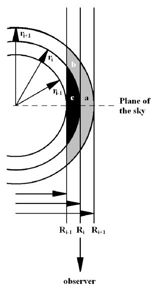
Figure 1: Illustration of the onion–skin model adopted for the geometrical deprojection (see text in Sect. 2.1; adapted from McLaughlin 1999).

The first method that we apply to recover the three–dimensional profiles of temperature and gas density is based on a geometrical technique originally introduced by Kriss et al. (1983), and subsequently adopted by (e.g., Buote, 2000; Ettori et al., 2002; Morandi et al., 2007) to deproject X–ray images and spectra of galaxy clusters. This method of geometrical deprojection is fully non–parametric and allows to reconstruct the 3-dimensional profile of a given quantity from its 2-dimensional observed projection, under the assumption of spherical symmetry.

Following Kriss et al. (1983), the cluster is assumed to have a onion–like structure (see Figure 1), with $N$ concentric spherical shells, each characterized by uniform gas density and temperature within it. Therefore, the cluster image in projection is divided into rings, which are generally assumed to have the same radii of the 3D spherical shells. Let us define $\epsilon_{i}$ as the signal to be recovered from the deprojection method within the $i$-th shell. In our analysis $\epsilon_{i}$ will be proportional to either $n_{e}T_{e}$ for the tSZ signal, or to $n_{e}^{2}\Lambda(T)$ for the X–ray emissivity. In this way, the contribution of the $i$-th shell to the surface brightness in the ring $j$ of the image will be given by $s_{i,j}=\epsilon_{i}\cdot V_{i,j}/A_{j}$, where the matrix $V_{i,j}$ has as entries the values of the volume of the shell $i$ which is projected on the ring $j$, whose area is $A_{j}$. By definition, $s_{i,j}=0$ for $j>i$. Accordingly, the surface brightness $S^{\prime}_{j}$ in the ring $j$ can be obtained by summing up the contributions from all the shells,

$$S^{\prime}_{j}={1\over A_{j}}\sum_{i=j}^{N}s_{i,j}={1\over A_{j}}\sum_{i=j}^{N}\epsilon_{i}\cdot V_{i,j}\,,$$ (1)

where the sums extend over the $N$ radial bins. The deprojection amounts to invert the above equation, i.e. to recover the values of $\epsilon_{i}$ from the observed projected signal $S^{\prime}_{j}$. We refer to Figure 1 to illustrate how this deprojection is performed in practice. Let the shell $i$, limited by $r_{i}$ and $r_{i+1}$, be the outermost one. Then, from the surface brightness $S^{\prime}_{i}$ in the ring $i$ (limited by $R_{i}$ and $R_{i+1}$), one can directly compute the emissivity of the shell $i$ simply by knowing the volume of the region (a) and the area of the ring. In this case, the sum in eq. 1 has only the term $j=i=N$. The adjacent inner ring, having index $i-1$ and limited by $R_{i-1}$ and $R_{i}$, takes instead a contribution from both the $i-1$ and $i$ shells. The former is computed by multiplying the emissivity of that shell by the volume of the region (b). After subtracting it, the only remaining contribution is that of the sell $i-1$ from which the emissivity $\epsilon_{i-1}$ is computed. This procedure is then repeated from ring to ring down to the center of the cluster.

For this simple scheme to be applied, one requires to have images extended out to the true external edge of the cluster, i.e. out to the radius where the surface brightness goes virtually to zero. Clearly, this situation is never attained in practical applications for at least two reasons. First, clusters are always embedded in a large–scale cosmic web, which makes it difficult to define a sharp outer boundary. Second, and more important, both instrumental and cosmic backgrounds often dominate the genuine signal from the cluster well before its virial boundary is reached.

To overcome this problem, it is then necessary to take into account the emission from the gas, which extends outside the $N$-th shell. This emission does not have a corresponding ring in the image but can give a non–negligible contribution to the surface brightness in all rings. To account for this contribution, we follow the approach of McLaughlin (1999), who modeled the volume emission from the gas beyond the last observable annulus as a power law, $\epsilon(r)\propto r^{-\alpha}$ (we refer to their Appendix A for a more detailed description). The idea behind this method is that the exact contribution to each ring from the external part can be calculated by integrating the volume emission $\epsilon(r)$. Then, the normalization of the power law shape of $\epsilon(r)$ is fixed by the requirement of matching the total surface brightness of the last ring. This correction can be expressed as an additional term to eq.(1), which is proportional to the surface brightness of the last ring:

$$S_{j}=S^{\prime}_{j}+f_{j}\cdot S_{N}\,,$$ (2)

Here, $f_{j}$ is a geometrical factor which is uniquely specified by the values of the limiting radii of the $j$-th ring and by the exponent $\alpha$. Eq.(2) must be actually interpreted as a set of $2N$ equations, which corresponds to the separate deprojection of the tSZ and of the X–ray signal, each performed for $N$ radial bins. The geometrical deprojection is then performed by inverting each set of $N$ equations, starting from the outermost bin and proceeding inward. This procedure provides the radial profiles of $n_{e}T_{e}$ and of $n_{e}^{2}\Lambda(T)$, whose combination finally gives the 3D profiles of electron number density and of temperature. We emphasize that the temperature so obtained is the actual electron temperature and not the deprojected spectroscopic temperature, usually obtained from the fitting of X–ray spectra.

Given the iterative nature of this procedure, the uncertainty associated to each ring propagates not only to the corresponding 3D shell, but also to all the inner shells. For this reason, it is very difficult with this method to have a rigorous derivation of the statistical uncertainties associated to the deprojected profiles. This is particularly true for the X–ray profiles, that also involve a derivative of the cooling function with respect to the temperature. The commonly adopted solution is based on realizing MonteCarlo simulations, over which to compute the errors (e.g. Ettori et al., 2002).

Furthermore, errors associated to different radial bins are not independent. This is due to the fact that the projected signal in a given ring is contributed by several shells. The resulting covariance in the signals recovered in different shells is not provided by this deprojection method. This is a rather important point on which we will come back in Section 4.

2.2 The maximum likelihood deprojection

This technique is based on performing the deprojection by maximizing a likelihood function, which is computed by comparing the observed tSZ and X–ray profiles with the ones obtained by projecting the onion–skin model in the plane of the sky. This approach offers more than one advantage with respect to the geometrical deprojection, described in the previous section. First, the deprojection of both X–ray and tSZ profiles is performed simultaneously, directly obtaining the whole density and temperature profiles and their errors. Second, besides the variance, it is also possible to compute the correlation matrix for all parameters, without any extra computational cost. Finally, it is possible to introduce in the likelihood extra terms in order to improve the accuracy and robustness of the technique. As we shall describe in the following, we adopt a regularization technique, which is based on imposing a suitable constraint to the likelihood function, to smooth out spurious oscillations in the recovered profiles induced by the covariance in the parameter estimate.

The definition of the likelihood is the most important part of the whole procedure. We define a joint likelihood for the tSZ profile, $\mathcal{L}_{tSZ}$, and for the X–ray surface brightness profile, $\mathcal{L}_{Xray}$, also including a term associated to the regularization constraint, $\mathcal{L}_{reg}^{\lambda}$. Since these three terms are independent, the total likelihood is given by the product of the individual ones:

$$\mathcal{L}\equiv\mathcal{L}_{tSZ}\cdot\mathcal{L}_{Xray}\cdot\mathcal{L}_{reg}^{\lambda}.$$ (3)

For both the tSZ and the X–ray profiles, the take the Gaussian form for the likelihood,

$$ln(\mathcal{L}_{tSZ,X-ray})=-{1\over 2}\chi^{2}=-{1\over 2}\sum_{i}\left({O_{i}-M_{i}\over\sigma_{i}}\right)^{2},$$ (4)

where $O_{i}$ are the values of the profiles, in the $i$-th bin, measured from the maps, while $M_{i}(x)$ are the model–predicted profile values, as obtained for the set $x$ of parameters. Finally, $\sigma_{i}$ is the uncertainty on the measured values $O_{i}$.

While the Gaussian expression is adequate for the tSZ signal, its application for the X–ray, instead of the Poisson distribution, requires the number of photons sampling the surface brightness map in each radial shell to be large enough to neglect the Poisson noise. As we shall discuss in the following, even in the outermost rings, we always have at least 20 photons in the “noisy” X–ray maps.

For the regularization constraint, we adopt the Philips-Towmey regularization method (Bouchet, 1995, and references therein). This method has been already used also by Croston et al. (2006) to deproject X–ray imaging and spectral data. The method consists of minimizing the sum of the squares of the $k^{th}$-order derivatives around each data-point, so as to smooth out oscillations in the profiles. Here we choose to minimize the second–order derivative, since we aim to eliminate fluctuations in the profiles, but not the overall gradient. As we shall discuss in the following, such oscillations are due either to genuine substructures or to noise which propagates from adjacent bins in the deprojection. The local derivative of the function $x_{i}$ at the $i$-th radial interval is computed by fitting it value and the values at the adjacent points, $x_{i-1}$ and $x_{i+1}$), with a second order polynomial. Let $r_{i}$ be the value of the equally–spaced cluster–centric distances, at which the profiles are sampled, and $\Delta_{r}$ the spacing. Then, the regularization likelihood can be cast in the form

$$ln(\mathcal{L}_{reg}^{\lambda})=-{1\over 2}\lambda^{\prime}\sum_{i=3}^{N-1}\left({2f_{i}-f_{i-1}-f_{i+1}\over\Delta_{x}^{2}}\right)^{2}\equiv$$

$$\equiv-\lambda\sum_{i=3}^{N-1}\left({2f_{i}-f_{i-1}-f_{i+1}}\right)^{2}$$ (5)

The quantity between parenthesis in the line formula is the exact value of the local second–order derivative around $r_{i}$. All the constant factors are included in the coefficient $\lambda$, which is called the regularity parameter. The choice of its value is determined by the compromise one wants to achieve between the fidelity to the data (low $\lambda$) and the regularity of the solution (high $\lambda$). A small $\lambda$ value will give an inefficient regularization, while a too high $\lambda$ will force the profile to a straight line, especially if the signal-to-noise ratio, S/N, is low. We apply the regularization constraint only to the temperature profile, which is that generally showing large oscillations, while the density profile has always a rather smooth shape. The sum in eq.(5) starts from $i=3$ since we prefer to exclude the innermost point from the regularization procedure.

With this approach, the values of the 3D gas density and temperature profiles are computed at $N=15$ radii each. Therefore, the total number of parameters to be determined with the maximum likelihood approach is 30. In order to optimize the sampling of such a large parameter space, we adopt a Markov Chain Monte Carlo (MCMC) fitting technique (Neal, 1993; Gilks et al., 1996; MacKay, 1996).

What the MCMC computes is the (marginalized) distribution of each parameter of a set, $x_{i}$ (i.e. the values of density and temperature into each bin), for which the global (posterior) probability $P(x)$, which is proportional to the likelihood function, is known at any point in the parameter space. In the case of an high number of parameters or of a particularly complex $P(x)$, this is quite difficult to be done analytically, or simply computationally very expensive. Instead, the MCMC performs the exploration of the parameter space with a limited computational cost, thanks to an iterative Monte Carlo approach, by sampling the $P(x)$ distribution. At each iteration, new values of the parameters are drawn from a symmetric proposal distribution, that in our case is a Gaussian,

$$q(x_{i},\hat{x}_{i})\propto e^{-{(x_{i}-\hat{x}_{i})}^{2}/2\alpha_{i}^{2}}\,.$$ (6)

Here $x_{i}$ and $\hat{x}_{i}$ are the entries of two vectors, having 30 components each, which represent the updated and the old values of the fitting parameters, respectively. The parameter $\alpha_{i}$ determines the possible range for $x_{i}$ given $\hat{x}$ .

After the likelihood function is computed for a new set of parameters $x$, these new values are accepted or rejected with a probability (A) given by the so–called Metropolis criterion (Metropolis et al., 1953):

$$A(x,\hat{x})=min\left\{1,{P(x)\over P(\hat{x})}\right\},$$ (7)

where $P(x)$ is the distribution sampled by the MCMC .

The width of the proposal distribution appearing in eq.(6), $\alpha_{i}$, determines the behavior of the chain: a small value of $\alpha_{i}$ increases the acceptance rate since the new proposed value is close to the old one, while a high value provides a faster exploration of the parameter space. Our criterion to choose the values of $\alpha_{i}$ is that the resulting acceptance rate, given by eq.(7), is around 10 per cent.

Each parameter is allowed to vary within a finite interval, in order to avoid that the MCMC finds secondary maxima in unphysical regions of the parameter space. As for gas density, we allow it to vary within a large range, $0.1<n_{e}<10^{-6}$ cm^-3. Since density is mostly constrained by the X–ray signal, which is proportional to $n_{e}^{2}$, it is always fairly well constrained and the above large interval of variation does not create convergence problems in any of our objects. The upper and lower limits allowed for the temperature are 25 keV (never reached along the chain) and 0.5 keV. Even though none of our clusters reach such low temperatures within the virial radius, the exploration of the parameter space during the Markov Chain run could reach such a low temperature regime. When this happens, the rapid drop of the cooling function $\Lambda(T)$ below 0.5 keV generates a maximum in the likelihood probability distribution, with unphysically low temperature and very high density.

The iterative procedure described above is repeated until a suitable number of new sets of parameters are accepted in the chain (typically $\raise-2.0pt\hbox{\hbox to0.0pt{\hbox{$\sim$}\hss}\raise 5.0pt\hbox{$>$}\ }5\times 10^{4}$). In this condition, the frequency of the occurrence in the chain of the $i$-th parameter $x_{i}$ approaches its true probability distribution, $P(x_{i})$. Note that each parameter distribution is already marginalized over the distributions of all the other parameters.

We perform the statistical analysis of the chain by using the code getdist of the COSMOMC package (Lewis & Bridle, 2002). In addition to a complete statistical analysis of the chain, the code performs a series of convergence tests: the Gelman & Rubin R statistics (Gelman & Rubin, 1992), the Raftery & Lewis test (Raftery, 2003) and a split–test (which essentially consists in splitting the chain into 2, 3 or 4 parts and comparing the difference in the parameter quantiles). We check the convergence of our result against all these three tests.

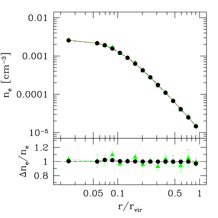
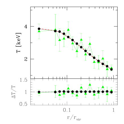
Figure 2: Results of the geometrical deprojection of the analytical model: density profile (left panel), temperature profile (right panel). The dashed line represents the true profile. The circles (triangles) connected by a solid line represent the reconstructed profiles without (with) the inclusion of the noise. Errorbars represent 1$\sigma$ deviations over 1000 Monte Carlo resamplings over the data (see text for details, Section 3.1)

3 Application to an idealized cluster model

In order to investigate the presence of possible systematics in the geometrical deprojection technique, we carry out a test on an ideal cluster model. We construct this model cluster by assuming the $\beta$–model for the gas density profile, with an effective polytropic equation of state to define the temperature profile:

$$n_{e} = n_{e0}\left(1+{r^{2}\over r_{c}^{2}}\right)^{-3\beta/2}$$

$$T = T_{0}\left({n_{e}\over n_{e0}}\right)^{\gamma-1}=T_{0}\left(1+{r^{2}\over r_{c}^{2}}\right)^{-3\beta(\gamma-1)/2}$$ (9)

The values of the model parameters are fixed as follows: $\beta=0.8$, $\gamma=1.2$ for the effective polytropic index, $n_{e0}=3\cdot 10^{-3}$ cm^-3 for central electron number density, $T_{0}=4$ keV for the central temperature, $r_{c}=200$ kpc for the core radius. The “virial” radius, which represents here the largest cluster-centric distance out to which the profiles are followed, is fixed at $r_{vir}=2$ Mpc. We assume the cluster to be placed at redshift $z=0.1$.

We create tSZ and X–ray images of this model in X–ray and tSZ. The maps are composed by a grid 512x512 pixels. The physical dimension of the pixel is $\sim 16$ kpc, which corresponds to an angular scale of $\sim 4$ arcsec at this redshift. In realizing the map of X–ray surface brightness, we adopt for the cooling function the pure bremsstrahlung expression $\Lambda(T)=\Lambda_{0}(T/T_{0})^{0.5}$ where $\Lambda_{0}=5\cdot 10^{-23}$ erg/s cm³. We prefer this simple formula since at this stage our main interest is to investigate the systematics of the deprojection itself, rather than the uncertainties introduced by the dependence of the X–ray emissivity on the temperature (which we expect anyway to be quite small).

We adopt the same binning strategy for both the ideal cluster and for the simulated objects, that we shall describe in the next Section. The first bin is taken from $r=0$ to $r=0.05r_{vir}$ which always corresponds to $\sim$$>$ 100 kpc in our set of simulated clusters. Then, we compute the profile in 10 (15) bins out to $R_{500}$ ($R_{vir}$) which are equally spaced in logarithm. This choice represents a good compromise between the needs of accurately resolving the profile and of having an adequate signal-to-noise (S/N $\sim$$>$ 5) in each bin. We point out that a proper binning criterion is important in order to get an unbiased reconstruction of the profiles. One should keep in mind that the spherical shells are assumed to have homogeneous gas density and temperature structures, thus neglecting any internal radial gradient. On the other hand, the portion of each shell, which is projected on the corresponding ring in the image, is located at a larger radial distance from the center than the portion of the same shell which is projected into the inner rings. Therefore, if the bin width is comparable or larger larger than the scale length of the internal radial gradient of the shell, the emissivity contributed to the correspondent ring is lower than expected from a homogeneous gas density, while it is larger for all the inner rings. As a consequence, the emissivity of the shell is underestimated while that of all the inner shells is overestimated in order to correctly reproduce the cluster image.

In order to check for the presence of such systematics, we first apply the deprojection technique in the case of an ideal observation, free of any noise. The reconstructed density and temperature profiles are shown in Figure 2. The reconstruction in this extremely idealized case is excellent, with very small or no deviations in all bins. Larger deviations are in the outermost bins and are related to the subtraction of the contribution of the fore–background contaminations. This contamination is due to the fact that the $\beta$–model used to produce our maps ideally extends out to infinity. Nevertheless, all deviations are smaller than a few percent and are negligible with respect to any observational noise. The results obtained in this test case show that taking equally log-spaced bins is in fact a good choice.

3.1 Geometrical deprojection of the noisy maps

The case of noiseless observations discussed in the previous section is highly idealized. The impact of including a realistic noise is instead very important and cannot be neglected. The recipe to add noise to the maps, that we describe here, will also be used in the study of the simulated clusters, discussed in Section 4.

As already mentioned in the Introduction, recovering detailed temperature profiles from the combination of X–ray imaging and tSZ data requires both of them to have an adequate spatial resolution. While this is certainly the case for the present generation of X–ray satellites, the combination of good sensitivity and spatial resolution for tSZ observations should await the next generation of sub-millimetric telescopes. For the purpose of our analysis, we model the noise in the tSZ maps by using as a reference the performances expected for the planned Cornell–Caltech Atacama Telescope (CCAT), which is expected to start operating at the beginning of the next decade(Sebring et al., 2006). The telescope will be a single–dish with 25 m diameter. The required field–of–view is of about $10\times 10$ arcmin², with the goal of covering a four times larger area, so as to cover one entire rich cluster down to a relatively low redshift. The best band for tSZ observations will be centered on 150 GHz. At this frequency CCAT is expected to have Gaussian beam of 0.44 arcmin FWHM. The first step of noise setup is to convolve the maps with this beam. Then we add a Gaussian noise of 3$\mu$K/beam. This level of noise should be reached with about 6 hours of exposure with CCAT. In the present study, we neglect in the tSZ maps any contamination, in particular we do not consider the presence of unresolved radio point sources. A detailed analysis of the contaminations in the tSZ signal has been provided by Knox et al. (2004) and by Aghanim et al. (2004).

As for X–ray observations, the Chandra satellite is currently providing imaging of superb quality, with a sub–arcsec resolution on axis. A proper simulation of X–ray observations should require generating spectra for each pixel, to be convolved with the response function of a given instrument. However, in order to apply our reconstruction method we only need to generate X-ray surface brightness maps with a given number of events (photons), regardless of their energy. For this purpose we simulate the X–ray photon counts by using a Monte Carlo sampling of the surface brightness map. We fix to $N=10^{4}$ the total number of photons within the virial radius of the cluster, which is quite typical for medium–deep observations of relatively nearby clusters. Each photon event is generated in a particular pixel $i$, with probability

$$P_{i}={s_{i}\over\sum_{j}s_{j}},$$ (10)

where $s_{i}$ is the surface brightness of the pixel and the sum is extended to all the pixels of the map. The number of expected counts into each pixel will be given by a Poisson probability distribution with mean $n_{i}=NP_{i}$. The conversion between counts and surface brightness is then given by $\Sigma=\sum_{i}s_{i}/N$, so that the total flux in the map is conserved.

Clearly, this method of introducing noise in the X–ray maps only takes into account the statistical errors associated to finite exposures. However, it neglects the effects of any systematics (e.g., contribution of the instrumental and cosmic background, etc.) which should be included in a more realistic observational setup. A comprehensive description of the instrumental effects on the recovery of X–ray observables, calibrated on hydrodynamical simulations, has been provided by Gardini et al. (2004) (see also Rasia et al., 2006). Probably the most serious limitation in our approach is that we assume the absence of any background or, equivalently, that the background can be characterized and removed with arbitrary accuracy.

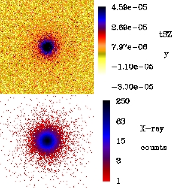
Figure 3: tSZ (upper panel) and X–ray (lower panel) maps of the ideal cluster. The side of the map corresponds to $2R_{vir}=4$ Mpc. In the bottom left corner of the tSZ map is the beam. Note that the scale is linear in the tSZ map and logarithmic in the X–ray one.

In Figure 3 we show are the tSZ and X–ray images of the idealized cluster, once noise is added as described above. In Figure 2 we show the results of the deprojection of the noisy maps of the idealized cluster, for both the density and the temperature profiles. In order to estimate the errors in the deprojected profiles, we perform a MonteCarlo resampling of the projected X–ray and tSZ profiles: the value of the profile within each radial ring is randomly scattered according to a Gaussian distribution, whose width is given by the error associated to the noise introduced in the map. The 1$\sigma$ errors in the deprojected profiles is then obtained as the scatter within a set of 1000 deprojections of the MonteCarlo–resampled tSZ and X–ray profiles.

The density is the best determined quantity, with uncertainty lower than 10 per cent. This is quite expected, owing to the sensitive dependence on gas density of both the X–ray signal ($\propto n_{e}^{2}$) and of the tSZ one ($\propto n_{e}$). The temperature has instead higher errors, of about 20–30 per cent. This is due to the fact that the X–ray signal has a weaker dependence on the temperature (only contained in the cooling function $\Lambda(T)$). For this reason, the determination of the temperature profile, independent of any X–ray spectroscopic analysis, is strictly related to the possibility of having high–quality tSZ data.

The introduction of noise generates fluctuations in the tSZ and X–ray profiles which translate into variations of the recovered density and temperature. Looking at the bottom panels of Fig. 2, positive fluctuations in the density correspond to negative fluctuations in the temperature (and viceversa). Furthermore, any fluctuation in a given direction in one radial bin generally corresponds to a fluctuation in the opposite direction in an adjacent bin, within the same profile. This pattern in the fluctuations witnesses the presence of a significant covariance among nearby bins in the same profile and between the values of density and temperature recovered within the same radial bin. As for the covariance between neighbor bins, it is due to the onion–skin structure assumed in the deprojection: every time that a quantity is over(under)estimated in a radial bin, the deprojection forces the same quantity to be under(over)estimated in the adjacent inner bin, so as to generate the correct projected profile. As for the covariance between different profiles, it is mostly induced by the tSZ signal, which has the same dependence on both $n_{e}$ and $T$. Although such oscillations are present for both density and temperature, they are smaller for the former, due to its faster decrease with radius.

3.2 Maximum likelihood deprojection of the noisy maps

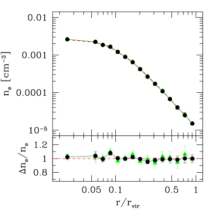
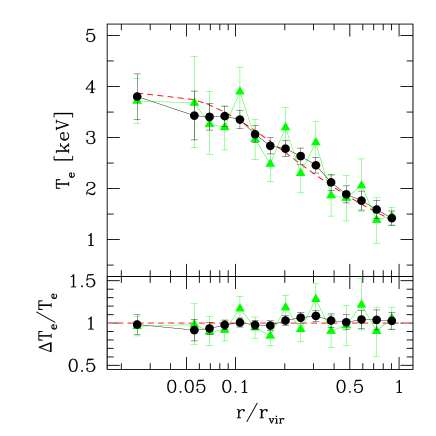
Figure 4: Results of the maximum–likelihood deprojection on the density profile (left panel) and temperature profile (right panel) for the idealized cluster. In the upper part of each panel we show the correct profile (dashed curve) and the reconstructed profile with and without the regularization constraint (circles and triangles, respectively). In the lower part we show the fractional deviation of the recovered profiles from the true one.

We verified that using the maximum–likelihood technique, as described in Sect. 2.2, generally produces very similar results to those of the geometrical deprojection, at least when the regularization term, $\mathcal{L}_{reg}^{\lambda}$ is not included in the analysis. The results of this deprojection method on the polytropic $\beta$-model are shown in Figure 4, where we also show the effect of introducing the regularization term. The effect of the regularization constraint is evident: most of the fluctuations, which are due to the degeneracies between fitting parameters, disappear and the deprojected profiles become much more regular, and with smaller errorbars in the profiles, while the accuracy of the reconstruction remains essentially unbiased.

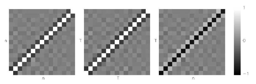
Figure 5: The correlation matrix of density and temperature without the regularization constraint: density-density (left panel), temperature-temperature (central panel) and density-temperature (right panel). White pixels correspond to the presence of strong positive correlation, while black pixels are for strong anti–correlation.

Figure 6: The correlation matrix of density and temperature while using regularization constraint: density-density (left panel), temperature-temperature (central panel) and density temperature (right panel). The color-coding of the pixels is the same as in Figure 5.

In order to study in detail the presence of correlations among the fitting parameters, we compute the correlation matrix, which is defined as $C_{ij}=\sigma_{ij}/\sigma_{i}\sigma_{j}$, where $\sigma_{ij}$ is the covariance between the $x_{i}$ and the $x_{j}$ fitting parameters, while $\sigma_{i}^{2}$ is the variance for the $x_{i}$ parameter. The covariance matrix is computed along the Markov Chain. Therefore, $C_{ij}$ is in our case a matrix with $30\times 30$ entries. In Figures 5 and 6 we plot the entries of the correlation matrix for the density–density (DD), temperature–temperature (TT) and density–temperature (DT) “blocks”, before and after introducing the regularization term in the likelihood function, respectively. By definition, the variance terms in the diagonal of the DD and TT matrices are characterized by the maximum correlation. On the contrary, the diagonal of the DT matrix has the maximum anticorrelation, thus demonstrating that any positive fluctuation in the recovered profile of one quantity corresponds to a negative fluctuation of the other quantity at the same radius. We also note that the next-to-diagonal terms in the DD and TT blocks have a degree on anticorrelation, thus explaining the fluctuating profile shown in Figs. 2 and 4. When the regularization is introduced, the correlations between density or temperature of adjacent bins is efficiently suppressed.

4 Application to simulated clusters

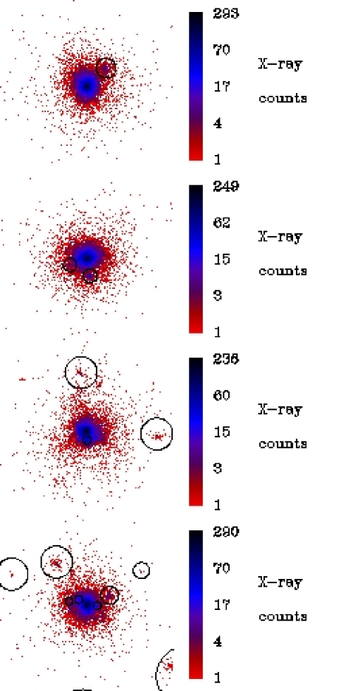
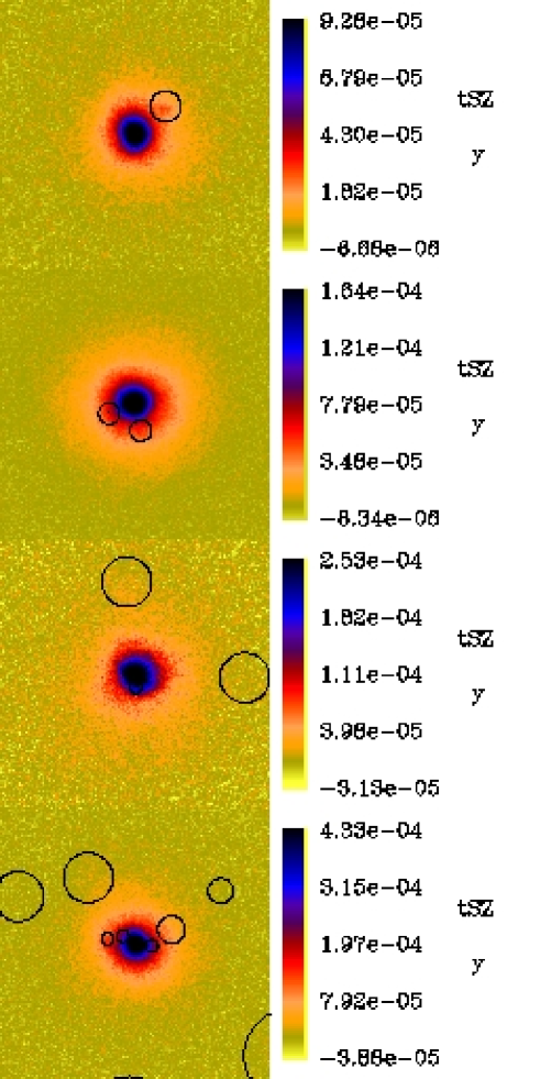
Figure 7: Maps of the X–ray surface brightness (left panel) and of the Comptonization parameter (right panel) for the C1 to C4 simulated clusters (from top to bottom). Each map extends out to $R_{vir}$. Noise is added according to the recipe described in Section 3.1. Circles mark the regions which have been masked, due to the presence of detected substructures.

The sample of simulated galaxy clusters used in this paper has been extracted from the large-scale cosmological hydro-N-body simulation of a “concordance” $\Lambda$CDM model with $\Omega_{m}=0.3$ for the matter density parameter at present time, $\Omega_{\Lambda}=0.7$ for the cosmological constant term, $\Omega_{\rm b}=0.019\,h^{-2}$ for the baryons density parameter, $h=0.7$ for the Hubble constant in units of 100 km s^-1Mpc^-1 and $\sigma_{8}=0.8$ for the r.m.s. density perturbation within a top–hat sphere having comoving radius of $8\,h^{-1}{\rm Mpc}$ (see Borgani et al. 2004, for further details). The run, performed with the Tree+SPH code GADGET-2 (Springel et al., 2001; Springel, 2005), follows the evolution of $480^{3}$ dark matter particles and an equal number of gas particles in a periodic cube of size $192h^{-1}$ Mpc. The mass of the gas particles is $m_{\rm gas}=6.9\times 10^{8}h^{-1}M_{\odot}$, and the Plummer-equivalent force softening is $7.5h^{-1}$ kpc at $z=0$. The simulation includes the treatment of radiative cooling, a uniform time–dependent UV background, a sub–resolution model for star formation and energy feedback from galactic winds (Springel & Hernquist, 2003). The sample of clusters analyzed here includes 14 clusters extracted at $z=0$ and having virial mass $M_{vir}\raise-2.0pt\hbox{\hbox to0.0pt{\hbox{$\sim$}\hss}\raise 5.0pt\hbox{$>$}\ }4\times 10^{14}M_{\odot}$. For these clusters we compute the electron temperature,

$$T_{e}\,=\,{\sum_{i}m_{i}T_{i}\over\sum_{i}m_{i}}\,,$$ (11)

whose definition coincides with the mass–weighted one under the assumption of a fully ionized plasma. In the above equation, $m_{i}$ and $t_{i}$ are the mass and the temperature of the $i$-th gas particle.

Due to the finite box size, the largest cluster found in the cosmological simulation has $T_{e}\approx 5$ keV. In order to extend our analysis to more massive and hotter systems, which are mostly relevant for current tSZ observations, we include four more galaxy clusters having $M_{\rm vir}>10^{15}\,h^{-1}M_{\odot}$ and belonging to a different set of hydro-N-body simulations (Borgani et al., 2006). Since these objects have been obtained by re-simulating, at high resolution, Lagrangian regions of a pre-existing cosmological simulation (Yoshida et al., 2001), they have a better mass resolution, with $m_{\rm gas}=1.69\times 10^{8}h^{-1}M_{\odot}$, and a correspondingly smaller softening of $5h^{-1}$kpc at $z=0$. These simulations have been performed with the same choice of the parameters defining star–formation and feedback. The cosmological parameters also are the same, except for a higher power spectrum normalization, $\sigma_{8}=0.9$.

Cluster $T_{e}$ $M_{vir}$ $R_{vir}$ keV $10^{14}M_{\odot}$ Mpc C1 2.5 4.0 2.1 C2 4.3 10.1 2.6 C3 5.5 26.6 3.1 C4 7.0 30.5 3.3

Table 1: Characteristics of the simulated clusters, for which the detail of the analysis are presented. Col. 1: electron (mass–weighted) temperature; Col. 3: virial mass; Col. 4: virial radius.

In the following, we will show detailed results for a subset of 4 clusters. The basic characteristics of these four selected clusters are reported in Table 1. The first three of them are extracted from the cosmological hydrodynamical simulation, while C4 is one of the massive clusters simulated at higher resolution. C2, C3 and C4 are typical examples of clusters at low, intermediate and high temperature, while C1 is an interesting case to understand the effect of fore–background contaminations. We show in Figure 7 the X–ray surface brightness and Compton–$y$ maps for these four clusters. All the maps are generated by placing the cluster at redshift $z=0.1$, so that the maps, which extend out to $r_{vir}$, have an angular size ranging from about 9 arcmin for C1 to 14 arcmin for C4.

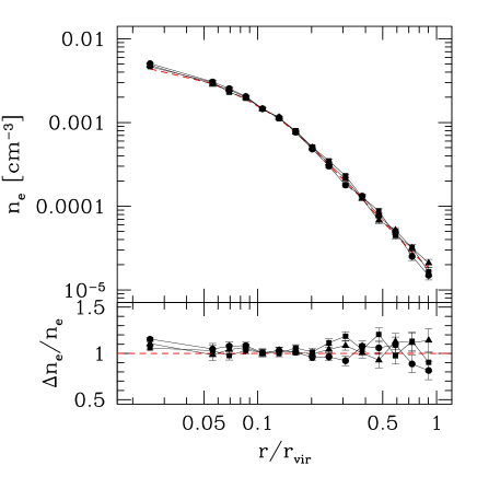
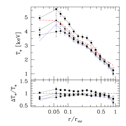
Figure 8: Application of the regularized maximum likelihood deprojection on the cluster C1, out to $R_{vir}$. The tree solid lines connecting dots with errorbars represent the reconstructed profile, for three orthogonal projection directions: along the $x$ (squares), the $y$ (triangles) and the $z$ (circles) axes. Errorbars corresponds the asymmetric 68 per cent confidence levels, computed from the distribution of values taken by the likelihood function along the Markov Chain. The dashed line represents the true 3-dimensional profile. The dotted line in the right panel shows the profile of the spectroscopic–like temperature. In the bottom panels, we plot the fractional deviation of the reconstructed profiles from the true electron temperature.

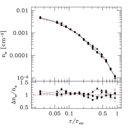
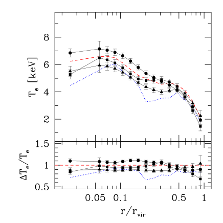
Figure 9: The same as in Figure 8, but for the C2 cluster.

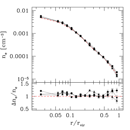
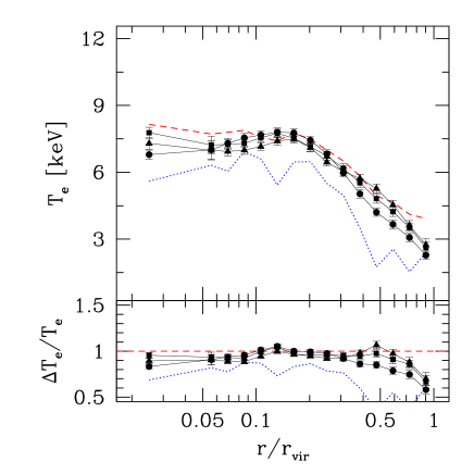
Figure 10: The same as in Figure 8, but for the C3 cluster.

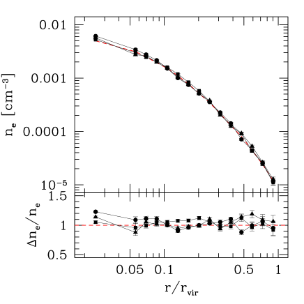
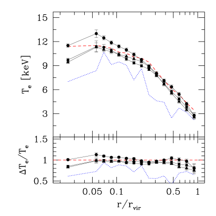
Figure 11: The same as in Figure 8, but for the C4 cluster.

4.1 tSZ and X–ray maps

Around each cluster we extract a spherical region extending out to 6 $R_{vir}$. Following Diaferio et al. (2005), we create maps of the relevant quantities along three orthogonal directions, extending out to about 2 $R_{vir}$ from the cluster center, by using a regular $512\times 512$ grid.

A number of different analyses, based on a joint deprojections of SZ and X–ray cluster maps under the assumption of axial symmetry, indicate that the X–ray selection tends to favor objects which are elongated along the line-of-sight (e.g., De Filippis et al., 2005, , and references therein). In order to control the effect of this selection bias, we decided to choose the axes of projection to be aligned with the principal axes of inertia of the cluster. This will allow us to quantify the difference in the reconstructed profiles when the projection direction is that of maximum cluster elongation.

To derive these axes, we diagonalize the inertia tensor, which is given by

$$I_{ij}=\sum_{p=0}^{N}(r_{i}r_{j})\rho_{p}^{2}$$ (12)

where $i,j=0,1,2$ are the coordinate axes, $r_{i}$ is the $i$-th coordinate of the particle $p$ with density $\rho_{p}$ and the sum is extended over all the gas particles. We weight each particle by $\rho_{p}^{2}$ so as to mimic the elongation in the X–ray emissivity.

The eigenvectors of the $I$ tensor provide the principal axes of the best–fitting ellipsoid. The semi–axes $a_{i}$ of this ellipsoid are proportional to square root of the corresponding eigenvalue $a_{i}\propto\sqrt{\lambda}_{i}$ (e.g. Plionis et al., 1991). We choose the direction of projection $z$ to be that corresponding to the largest semi–axis (i.e. the maximum elongation), while the $y$ and $x$ directions correspond to the medium and to the lower semi–axes, respectively.

In the Tree+SPH code, each gas particle has a smoothing length $h_{i}$ and the thermodynamical quantities it carries are distributed within the sphere of radius $h_{i}$ according to the compact kernel:

$$W(x)=\frac{8}{\pi h_{i}^{3}}\left\{\begin{array}[]{ll}1-6x^{2}+6x^{3}&0\leq x\leq\frac{1}{2}\\ 2(1-x)^{3}&\frac{1}{2}\leq x\leq 1\\ 0&x\geq 1\end{array}\right.$$ (13)

Here, it is $x=r/h_{i}$ with $r$ the distance from the particle position. Therefore, we distribute the quantity of each particle on the grid points within the circle of radius $h_{i}$ centered on the particle. Specifically, we compute a generic quantity $q_{jk}$ on the $(j,k)$ grid point as $q_{jk}d^{2}_{p}=\int q(r)dld^{2}_{p}=\sum q_{i}(m_{i}/\rho_{i})w_{i}$ where $d^{2}_{p}$ is the pixel area, the sum runs over all the particles, and $w_{i}\propto\int W(x)dl$ is the weight proportional to the fraction of the particle proper volume, $m_{i}/\rho_{i}$, which contributes to the $(j,k)$ grid point. For each particle, the weights $w_{k}$ are normalized to satisfy the relation $\sum w_{k}=1$ where the sum is over the grid points within the particle circle. When $h_{i}$ is so small that the circle contains no grid point, the particle quantity is fully assigned to the closest grid point.

As for the X–ray maps, they have been generated in the [0.5-2] keV energy band, by computing the emissivity of each gas particle with a Raymond-Smith code (Raymond & Smith, 1977), assuming zero metallicity in the cooling function.

Noise is finally added as described in Section 3.1. We fix the total number of photons in the virial radius to $10^{4}$ also for simulated clusters. For the tSZ map, we adopt a noise level of 10 $\mu$K/beam for the objects having spectroscopic temperature $T_{sl}>4$ K and 3 $\mu$K/beam for those having $3$ K $<T_{sl}<4$ K.

4.2 Results

Having tested the reliability of the deprojection method, with the regularization of the likelihood, we apply now this technique to the more realistic case of hydrodynamical simulations. In this case, a number of effects, such as deviations from spherical symmetry, presence of substructures and presence of fore/background contaminating structures, are expected to degrade the capability of the deprojection to recover the three-dimensional profiles.

We show in detail the results on the density and temperature deprojection the selected subset of four clusters presented in Table 1 while the whole set of 14 clusters will be used to assess on a statistical basis the efficiency with which the total gas mass can be recovered.

The C2 and C4 objects are rather typical examples of our set of clusters. They are fairly relaxed and with a modest amount of substructures. As for the presence of substructures, they are well known to represent an important source of bias in the deprojection, especially of the X–ray signal, which is highly sensitive to gas clumping. In order to remove this contaminating signal, we follow the same method that is often adopted in the analysis of observational data. We first identify the detectable clumps by visual inspection of the X–ray maps. The corresponding regions are then masked out both in the X–ray and in the tSZ maps. The masked regions are excluded from the computation of the signals to be deprojected. This leads to an increase of the statistical uncertainties in those rings which have a significant overlap with the masked regions. Clearly, due to the finite photon statistics in the X–ray maps, small clumps may fall below the detection threshold, while their presence may still affect the emissivity.

The recovered density and temperature profiles of C2 and C4 are shown in Figures 9 and 11. Once all the detectable clumps are masked out the reconstruction of the density profile is generally good, but with a systematic overestimate of $\sim$5 per cent, that we attribute to a residual small–scale gas clumping. Although this effect is rather small, its presence highlights the need to have a sufficient photon–count statistics to identify gas inhomogeneities and remove their contribution in the deprojection procedure. The slight density overestimate corresponds, as expected, to a small underestimate of the temperature, which is forced by the requirement of reproducing the tSZ signal, $y\propto n_{e}T_{e}$. For these two objects we also note that there are rather small differences in the 3D profiles recovered from three orthogonal projection directions, thus indicating that they are almost spherical and without significant substructures along the different projection directions. Errorbars are always of the order of a few percent, in both density and temperature. We stress that these very small errorbars, especially in temperature, are partly a consequence of the regularization constraint.

As for the C3 cluster, we note that it has larger substructures which will have a stronger impact on the recovered profiles. Even after masking all the detectable substructures, we still have a number of unresolved clumps. As expected, in this case the density profile (see Figure 10) is overestimated by a larger factor, $\sim 10$ cent, with a corresponding more significant underestimate of the temperature. The deviations of the deprojected profiles in the outer parts are also larger. This is due to stronger contaminations from the fore/background structures, which are both placed at the outskirts of the cluster and along the projection direction, in the cosmic web surrounding the cluster. In fact, both tSZ and X–ray maps are produced by projecting a region of 6 $R_{vir}$ in front and in the back of the cluster center.

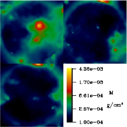
Figure 12: Projected surface gas mass density of the C1 cluster along the $z$ (top left), $y$ (top right) and $x$ (bottom left) directions, after removing the contribution from all gas particles which inside the virial region of the cluster.

In this respect, the C1 cluster is particularly interesting. Along the $x$-axis projection there is a merging groups along the same line of sight, at a distance of $\sim 1.2R_{vir}$ from the center of the main cluster. In Figure 12 we show the projected mass surface density of the gas along the three projection directions, after removing the mass of the main cluster within $R_{vir}$. While the residual mass surface density is quite small along the $x$ and $y$ directions, a presence of a gas clump are shows up in the $z$ projection. While this structure provides a rather small contribution to the X–ray signal, its gas pressure is comparable to that of the main cluster, thereby significantly contaminating the tSZ effect signal. As a consequence, the density profile (see Figure 8) is essentially unaffected, while the temperature is clearly boosted by $\sim 20$ per cent with respect to the that obtained from the other two projections. Although this is a quite peculiar case, in which the secondary structure is relatively large and aligned with the main cluster along the line of sight, it illustrates the role of projection contamination from unidentified structures in recovering the 3D thermal structure of the ICM.

We note in Figs.8–11 that the density profiles recovered from the projection of maximum elongation are overestimated at small radii, while they are underestimated in the outskirts. In order to quantify this effect, we show in the left panel of Figure 13 the ratio between the true and the reconstructed density profiles, after averaging over the sample of simulated clusters. By averaging over all the projection directions, the density is generally overestimated by about 5 per cent at all cluster radii. This result is confirmed also by analyses performed on synthetic X–ray observations of simulated clusters (Rasia et al., 2006; Nagai et al., 2007). On the other hand, the density profile reconstructed from the projection along the $z$ axis is confirmed to be significantly larger than along the other direction in the very inner part, with an inversion at $r\raise-2.0pt\hbox{\hbox to0.0pt{\hbox{$\sim$}\hss}\raise 5.0pt\hbox{$>$}\ }0.2r_{\rm vir}$. Indeed, the elongation causes the objects to appear more compact in the X–ray maps, which drive the density reconstruction. This boosts the deprojected central density, while depletes it in the outskirts.

As shown in the right panel of Fig. 13, the temperature is generally underestimated by $\sim$$<$ 10 per cent out to $\simeq 0.7r_{vir}$. At larger radii this underestimate increases, reaching a mean value of about 20 per cent at $r_{vir}$, as a consequence of the relatively larger contamination by fore/background structures. The scatter is generally larger than the uncertainty introduced by the noise, so that it has to be considered as intrinsic to the measure. This scatter has different origins, such as unresolved gas clumps, asphericity of the clusters, fore–background contaminations. In general, the temperature recovered from the projection along the $z$ axis is slightly larger than the one from the other two axes. The difference is more apparent in the central regions and becomes smaller in the outskirts. The reason for this behaviour is that the temperature reconstruction is more affected by the tSZ signal. Along the direction of maximum elongation, this signal in enhanced since the ICM pressure is integrated along a larger path. The tSZ signal receives then an important contribution from cluster regions where the density is underestimated. As a result the reconstructed temperature is correspondingly increased to compensate for this effect.

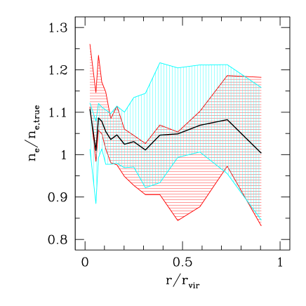
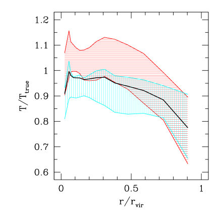
Figure 13: The ratio between the reconstructed and the true (mass–weighted) temperature and density profiles. The shaded areas encompass the $\pm 1\sigma$ regions of the recovered profiles over the ensemble of simulated clusters. The horizontally shaded area is for the projections along the $z$ axis, while the vertically shaded area is for the projections along the other two axes. The black line shows the mean over all projections of all clusters.

In Figs. 8–11 we also show the three–dimensional profile of the spectroscopic–like temperature (dotted line), which has been shown by Mazzotta et al. (2004) to represent a quite close proxy to the actual X–ray temperature obtained from a spectroscopic fit (see also Vikhlinin, 2006). This temperature is computed as

$$T_{sl}\,=\,{\sum_{i}\rho_{i}m_{i}T_{i}^{\alpha-1/2}\over\sum_{i}\rho_{i}m_{i}T_{i}^{\alpha-3/2}}\,,$$ (14)

with $\alpha\simeq 0.75$ and the sum extends over all the gas particles having internal energy larger than 0.5 keV. According to its definition, this temperature gives more weight to the low–temperature phase in a thermally complex ICM. This is the reason for the drop of the $T_{sl}$ profile at the cluster center and for the wiggles which mark the positions of merging sub-clumps which are relatively colder than the ambient ICM. In general, the profile of $T_{sl}$ are lower than those of the electron temperature, by an amount which is larger for hotter systems (see also Rasia et al., 2005). These figures highlight that the temperature profiles, as obtained from our deprojection analysis, are much closer to the mass–weighted temperature, which measures the total thermal content of the ICM, than to $T_{sl}$. An important consequence of this difference will clearly be the estimate of the total cluster mass from the application of hydrostatic equilibrium. We will discuss the application of our deprojection method to cluster mass estimates in a forthcoming paper.

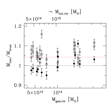
Figure 14: The ratio between the recovered and the true values of the total gas mass for simulated clusters out to For each cluster we show the result of the deprojection along the three orthogonal directions, with the projection corresponding to the maximum elongation being marked with a filled circle. Errorbars correspond to the $1\sigma$ confidence level, by accounting for the full error correlation matrix when integrating the 3D gas density profiles. The horizontal dotted line shows the average value of the ratio.

Figure 15: The same of figure 14, but as a function of cluster ellipticity (left panel), prolateness (central panel) and elongation along the line of sight (right panel).

4.3 Recovering the gas mass

As a first application of our deprojection procedure, we compute the gas mass of the clusters, which is calculated simply by summing up the mass contained into each radial bin. Since the bins are not independent, the errors on the total gas mass have been calculated by using both variances and covariances of the values of the density at different radii.

$$\sigma_{M}^{2}={1\over N-1}\sum_{i=0}^{N}\sum_{j=0}^{N}\sigma_{m,ij},$$ (15)

where $\sigma_{m,ij}$ is the covariance between the mass content of the $i$-th and of the $j$-th shells, directly obtained from the covariance between the gas density in different bins (e.g., see left panel of Fig. 6). Note that since the covariance between the density in adjacent bins is generally negative, neglecting it would lead to a systematic overestimate of the error on the mass.

We give the results on the estimate of gas mass for the whole set of 14 simulated clusters. The small overestimate found for the density profiles is obviously propagated to the estimate of the total gas mass. The resulting bias turns out to be very small, and amounts to about 4 percent, with no obvious trend with the cluster mass. This demonstrate that residual gas clumping, after the removal of the substructures identified in the X–ray maps, has a small effect on the our capability of the recovering the total mass of the ICM. We note that cluster-by-cluster variance is often comparable to the “projection variance”, i.e. to the differences found when projecting the same clusters along different directions. We also note that the uncertainties in the individual $M_{gas}$ estimates, typically of the order of a few per cent, are smaller than the scatter. This indicates that the intrinsic scatter in the recovered gas mass is in fact associated to the deviations of the simulated clusters from perfect spherical symmetry.

4.4 The effect of morphology

In order to better understand how morphology affects the deprojection, we plot in Figure 15 the recovered gas mass as a function of cluster ellipticity, prolateness and elongation along the line of sight. The ellipticity of a triaxial object is defined as:

$$\epsilon={1\over 2}{{1\over a_{min}}-{1\over a_{max}}\over{1\over a_{min}}+{1\over a_{med}}+{1\over a_{max}}}$$ (16)

and the prolateness as:

$$p={1\over 2}{{1\over a_{min}}-{2\over a_{med}}+{1\over a_{max}}\over{1\over a_{min}}+{1\over a_{med}}+{1\over a_{max}}}$$ (17)

The elongation is defined as the ratio between the semi–axis aligned with the line of sight and the larger of the other two semi–axes.

The gas mass recovered from the projection along the principal axis is generally lower than those from the other two projections. This underestimate generally is anticorrelated with the elongation of the cluster, although with a substantial scatter. From the left and the central panels of Figure 15, we do not find any significant correlation between the global 3D morphology of the clusters (prolateness and ellipticity) and the bias in the deprojection. Instead, as shown in the right panel, any effect in the gas mass recovery is driven by the orientation of the cluster.

5 Discussion and conclusions

We have presented results of deprojection methods, aimed at recovering the three-dimensional density and temperature profiles of galaxy clusters, by combining X–ray surface brightness and thermal SZ (tSZ) maps. The main aim of our analysis is to verify to what accuracy one can recover the thermal structure of the ICM by taking advantage of the different dependence of the X–ray and tSZ signal on the gas density and temperature, thereby avoiding performing X–ray spectroscopy. The two deprojection methods considered are both based on assuming spherical symmetry of the clusters.

The first one follows a geometrical approach, in which the 3D profiles are recovered with an iterative procedure that deprojects the observed images starting from the outermost ring and proceeding inwards. The second method assumes the values of the 3D gas density and temperature profiles at different radii and computes from them the expected SZ and X–ray surface brightness which is then compared to the observations with a maximum likelihood approach. In the computation of the likelihood, we also introduced a regularization term, which allows us to suppress spurious oscillations in the recovered profiles. Using a Monte Carlo Markov Chain (MCMC) approach to optimize the sampling of the parameter space, this second method also allows us to recover the full correlation matrix of the errors in the parameter fitting.

The main results of our analysis can be summarized as follows.

• The application of both methods to an idealized spherical polytropic $\beta$–model shows that the 3D profiles are always recovered with excellent precision (of about 3–4 per cent), thus demonstrating that such methods do not suffer from any intrinsic bias.

• The application of the maximum–likelihood method to hydrodynamical simulations of galaxy clusters always provides deprojected profiles of gas density and temperature, which are in good agreement with the true ones, out to the virial radius. We find a small ($\raise-2.0pt\hbox{\hbox to0.0pt{\hbox{$\sim$}\hss}\raise 5.0pt\hbox{$<$}\ }10$ per cent) systematic overestimate of the gas density, which is due to the presence of some residual gas clumping, which is not removed by masking out the obvious substructures identified in the X–ray maps.

• The total gas mass is recovered with a small bias of 4 per cent, with a sizable scatter of about 5 per cent. This result shows that residual gas clumping should have a minor impact in the estimate of the total gas mass. We do not find any trend in the recovery of the gas mass with the total cluster mass.

• The gas mass reconstructed along the maximum elongation axis is generally lower (by up to 10 per cent) with respect to the mass reconstructed along the other two projection axes, the size of this effect being larger for more elongated clusters.

• The temperature is generally well recovered, with $\sim 10$ per cent deviations from the true one out to $\simeq 0.7R_{\rm vir}$. The rather small size of this bias confirms that the combination with tSZ data is a valid alternative to X–ray spectroscopy for temperature measurements. The temperature reconstructed from the projection along the axis with maximum elongation is slightly higher than those from the other two axes, particularly in the inner regions.

Our results confirm the great potentials of combining spatially resolved tSZ and X–ray observations to recover the thermal structure of the ICM. This approach has several advantages with respect to the traditional one based on X–ray spectroscopy. First, the temperature recovered from the fit of the X–ray spectra is known to provide a biased estimate of the total thermal content of the ICM, the size of this bias increasing with the complexity of the plasma thermal structure (e.g., Mazzotta et al., 2004; Vikhlinin, 2006). Secondly, X–ray surface brightness profiles can be obtained with good precision with a relatively small number of photon counts. Also, once the cosmic and instrumental backgrounds are under control, the surface brightness can be recovered over a large portion of the cluster virial regions, as already demonstrated with ROSAT-PSPC imaging data (e.g., Vikhlinin et al., 1999; Neumann, 2005). Since the tSZ has the potential of covering a large range in gas density, then its combination with low–background X–ray imaging data will allow one to recover the temperature profiles out to the cluster’s outskirts.

A limitation of the analysis presented in this paper is that we did not include realistic backgrounds in the generation of the X–ray and tSZ maps. As we have just mentioned, there are reasonable perspectives for a good characterization of the X–ray background. However, the situation may be more complicated for the tSZ background. In this case, contaminating signals from unresolved point–like radio sources (e.g., Bartlett & Melin, 2006) and fore/background galaxy groups (e.g., Hallman et al., 2007) could affect the tSZ signal in the cluster outskirts. In this respect, the possibility of performing multi–frequency observations with good angular resolution will surely help in characterizing and removing these contaminations.

Single–dish sub-millimetric telescopes of the next generation promises to provide tSZ images of clusters with a spatial resolution of few tens of arcsec, while covering fairly large field of views, with 10–20 arcmin aside, with a good sensitivity. At the same time, planned satellites for X–ray surveys will have the capability of surveying large areas of the sky with a good quality imaging and control of the background. These observational facilities will open the possibility of carrying out in survey mode high–quality tSZ and X–ray imaging for a large number of clusters. The application of deprojection methods, like those presented in this paper will provide reliable determinations of the temperature profiles and, therefore, to exploit their potentiality as tools for precision cosmology.

References

- Aghanim et al. (2004) Aghanim N., Hansen S. H., Lagache G., 2004, ArXiv Astrophysics e-prints
- Ameglio et al. (2006) Ameglio S., Borgani S., Diaferio A., Dolag K., 2006, MNRAS, 369, 1459
- Bartlett & Melin (2006) Bartlett J. G., Melin J.-B., 2006, A&A, 447, 405
- Birkinshaw (1999) Birkinshaw M., 1999, Phys. Rep., 310, 97
- Bonamente et al. (2006) Bonamente M., Joy M. K., LaRoque S. J., Carlstrom J. E., Reese E. D., Dawson K. S., 2006, ApJ, 647, 25
- Borgani (2006) Borgani S., 2006, ArXiv Astrophysics e-prints
- Borgani et al. (2006) Borgani S., Dolag K., Murante G., Cheng L.-M., Springel V., Diaferio A., Moscardini L., Tormen G., Tornatore L., Tozzi P., 2006, MNRAS, pp 270–+
- Borgani et al. (2004) Borgani S., Murante G., Springel V., Diaferio A., Dolag K., Moscardini L., Tormen G., Tornatore L., Tozzi P., 2004, MNRAS, 348, 1078
- Bouchet (1995) Bouchet L., 1995, A&AS, 113, 167
- Buote (2000) Buote D. A., 2000, ApJ, 539, 172
- Carlstrom et al. (2002) Carlstrom J. E., Holder G. P., Reese E. D., 2002, ARAA, 40, 643
- Cavaliere & Fusco-Femiano (1976) Cavaliere A., Fusco-Femiano R., 1976, A&A, 49, 137
- Cavaliere & Lapi (2006) Cavaliere A., Lapi A., 2006, ApJ, 647, L5
- Croston et al. (2006) Croston J. H., Arnaud M., Pointecouteau E., Pratt G. W., 2006, A&A, 459, 1007
- De Filippis et al. (2005) De Filippis E., Sereno M., Bautz M. W., Longo G., 2005, ApJ, 625, 108
- Diaferio et al. (2005) Diaferio A., Borgani S., Moscardini L., Murante G., Dolag K., Springel V., Tormen G., Tornatore L., Tozzi P., 2005, MNRAS, 356, 1477
- Doré et al. (2001) Doré O., Bouchet F. R., Mellier Y., Teyssier R., 2001, A&A, 375, 14
- Ettori et al. (2002) Ettori S., De Grandi S., Molendi S., 2002, A&A, 391, 841
- Gardini et al. (2004) Gardini A., Rasia E., Mazzotta P., Tormen G., De Grandi S., Moscardini L., 2004, MNRAS, 351, 505
- Gelman & Rubin (1992) Gelman A., Rubin D., 1992, Stat. Science, 7, 457
- Gilks et al. (1996) Gilks W., Richardson S., Spiegelhalter D., 1996, Markov Chain Monte Carlo in practice. Chapman and Hall
- Hallman et al. (2007) Hallman E. J., O’Shea B. W., Burns J. O., Norman M. L., Harkness R., Wagner R., 2007, ArXiv e-prints, 704
- Hastings (1970) Hastings W., 1970, Biometrika, 57, 97
- Knox et al. (2004) Knox L., Holder G. P., Church S. E., 2004, ApJ, 612, 96
- Kotov & Vikhlinin (2006) Kotov O., Vikhlinin A., 2006, ApJ, 641, 752
- Kriss et al. (1983) Kriss G. A., Cioffi D. F., Canizares C. R., 1983, ApJ, 272, 439
- LaRoque et al. (2006) LaRoque S. J., Bonamente M., Carlstrom J. E., Joy M. K., Nagai D., Reese E. D., Dawson K. S., 2006, ApJ, 652, 917
- Lee & Suto (2004) Lee J., Suto Y., 2004, ApJ, 601, 599
- Lewis & Bridle (2002) Lewis A., Bridle S., 2002, Phys. Rev. D, 66, 103511
- MacKay (1996) MacKay D., 1996, Markov Chain Monte Carlo in practice. Chapman and Hall
- Mazzotta et al. (2004) Mazzotta P., Rasia E., Moscardini L., Tormen G., 2004, MNRAS, 354, 10
- McLaughlin (1999) McLaughlin D. E., 1999, AJ, 117, 2398
- Metropolis et al. (1953) Metropolis N., Rosenbluth A., Rosenbluth M., Teller A., Teller E., 1953, Journal of Chemical Physics, 21, 1087
- Morandi et al. (2007) Morandi A., Ettori S., Moscardini L., 2007, MNRAS, pp 541–+
- Nagai et al. (2007) Nagai D., Vikhlinin A., Kravtsov A. V., 2007, ApJ, 655, 98
- Neal (1993) Neal R. M., , 1993, Probabilistic inference using Markov Chain Monte Carlo methods
- Neumann (2005) Neumann D. M., 2005, A&A, 439, 465
- Piffaretti et al. (2005) Piffaretti R., Jetzer P., Kaastra J. S., Tamura T., 2005, A&A, 433, 101
- Plionis et al. (1991) Plionis M., Barrow J. D., Frenk C. S., 1991, MNRAS, 249, 662
- Pointecouteau et al. (2002) Pointecouteau E., Hattori M., Neumann D., Komatsu E., Matsuo H., Kuno N., Böhringer H., 2002, A&A, 387, 56
- Pratt & Arnaud (2005) Pratt G. W., Arnaud M., 2005, A&A, 429, 791
- Puchwein & Bartelmann (2006) Puchwein E., Bartelmann M., 2006, A&A, 455, 791
- Raftery (2003) Raftery 2003, Information Theory, Inference, and Learning Algorithms. Cambridge University Press (http://www.inference.phy.cam.ac.uk/mackay/itprnn/book.html
- Rasia et al. (2006) Rasia E., Ettori S., Moscardini L., Mazzotta P., Borgani S., Dolag K., Tormen G., Cheng L. M., Diaferio A., 2006, MNRAS, 369, 2013
- Rasia et al. (2005) Rasia E., Mazzotta P., Borgani S., Moscardini L., Dolag K., Tormen G., Diaferio A., Murante G., 2005, ApJ, 618, L1
- Raymond & Smith (1977) Raymond J. C., Smith B. W., 1977, ApJS, 35, 419
- Reblinsky (2000) Reblinsky K., 2000, A&A, 364, 377
- Rosati et al. (2002) Rosati P., Borgani S., Norman C., 2002, ARAA, 40, 539
- Sebring et al. (2006) Sebring T. A., Giovanelli R., Radford S., Zmuidzinas J., 2006, in Ground-based and Airborne Telescopes. Edited by Stepp, Larry M.. Proceedings of the SPIE, Volume 6267, pp. 62672C (2006). Cornell Caltech Atacama Telescope (CCAT): a 25-m aperture telescope above 5000-m altitude
- Sereno (2007) Sereno M., 2007, ArXiv e-prints, 707
- Springel (2005) Springel V., 2005, ArXiv Astrophysics e-prints
- Springel & Hernquist (2003) Springel V., Hernquist L., 2003, MNRAS, 339, 289
- Springel et al. (2001) Springel V., Yoshida N., White S., 2001, New Astronomy, 6, 79
- Sunyaev & Zeldovich (1972) Sunyaev R. A., Zeldovich Y. B., 1972, Comments on Astrophysics and Space Physics, 4, 173
- Vikhlinin (2006) Vikhlinin A., 2006, ApJ, 640, 710
- Vikhlinin et al. (1999) Vikhlinin A., Forman W., Jones C., 1999, ApJ, 525, 47
- Vikhlinin et al. (2005) Vikhlinin A., Markevitch M., Murray S. S., Jones C., Forman W., Van Speybroeck L., 2005, ApJ, 628, 655
- Voit (2005) Voit G. M., 2005, Reviews of Modern Physics, 77, 207
- Yoshida et al. (2001) Yoshida N., Sheth R., Diaferio A., 2001, MNRAS, 328, 669
- Zaroubi et al. (2001) Zaroubi S., Squires G., de Gasperis G., Evrard A. E., Hoffman Y., Silk J., 2001, ApJ, 561, 600
- Zaroubi et al. (1998) Zaroubi S., Squires G., Hoffman Y., Silk J., 1998, ApJ, 500, L87+
- Zhang & Wu (2000) Zhang T.-J., Wu X.-P., 2000, ApJ, 545, 141