Pattern formation in the damped Nikolaevskiy equation

Abstract

The Nikolaevskiy equation has been proposed as a model for seismic waves, electroconvection and weak turbulence; we show that it can also be used to model transverse instabilities of fronts. This equation possesses a large-scale “Goldstone” mode that significantly influences the stability of spatially periodic steady solutions; indeed, all such solutions are unstable at onset, and the equation exhibits so-called soft-mode turbulence. In many applications, a weak damping of this neutral mode will be present, and we study the influence of this damping on solutions to the Nikolaevskiy equation. We examine the transition to the usual Eckhaus instability as the damping of the large-scale mode is increased, through numerical calculation and weakly nonlinear analysis. The latter is accomplished using asymptotically consistent systems of coupled amplitude equations. We find that there is a critical value of the damping below which (for a given value of the supercriticality parameter) all periodic steady states are unstable. The last solutions to lose stability lie in a cusp close to the left-hand side of the marginal stability curve.

I Introduction

The Nikolaevskiy equation

$${\partial u\over\partial t}+u{\partial u\over\partial x}=-{\partial^{2}\over\partial x^{2}}\left(ru-\left(1+{\partial^{2}\over\partial x^{2}}\right)^{2}u\right)$$ (1)

has been widely studied, because of its application to several physical systems and its interesting nonlinear dynamics. It can also be written in the alternative form

$${\partial\phi\over\partial t}+\frac{1}{2}\left({\partial\phi\over\partial x}\right)^{2}=-{\partial^{2}\over\partial x^{2}}\left(r\phi-\left(1+{\partial^{2}\over\partial x^{2}}\right)^{2}\phi\right)$$ (2)

after introducing $u=\phi_{x}$.

The equation (1) was first derived, in an extended form, by Nikolaevskiy as a model for seismic waves in the earth’s crust ber ; nik . More recently, other applications of (1) or (2) have been proposed. Fujisaka and Yamada fy and Tanaka tan04 have derived (2) as a possible phase equation arising in reaction–diffusion systems. Turbulence in electroconvection was studied experimentally by Hidaka et al. hia , who proposed that the chaotic dynamics was of a type described qualitatively by (1). More generally, the Nikolaevskiy equation can be regarded as a canonical model for a pattern-forming system with the additional feature of symmetry under the transformation $\phi\to\phi+{}$constant, in the form (2) trt , or with Galilean symmetry, in the form (1) mat . Therefore, (1) is a suitable model for pattern-forming systems with these additional symmetries. Finally, as we show in Section II below, (2) can be used to describe finite-wavelength instabilities of travelling fronts.

The Nikolaevskiy equation exemplifies what is known as “soft-mode turbulence”. This form of chaotic dynamics arises from the interaction between a pattern of finite wavenumber, which appears for $r>0$, and a long-wave neutral (or “Goldstone”) mode. The neutral mode arises as a direct consequence of the additional symmetries discussed above. In a sufficiently large domain, all spatially periodic steady states are unstable, as was shown by Tribelsky and Velarde triv , and numerical investigations of (1) show irregular chaotic patterns mat ; trt ; st07 . In Ref. mat we showed that in this turbulent regime, (1) exhibits an unusual scaling, with the amplitude of $u$ proportional to the $3/4$ power of the supercriticality parameter $r$, whereas it is more usually proportional to the $1/2$ power in other pattern-forming systems. Fujisaka et al. fhy extended (2) to two spatial dimensions and found that this same scaling law holds.

In this paper, we consider the effect of adding a weak damping term to the neutral mode in (1). The motivation for this is that in real experimental systems, the symmetry that gives rise to the neutral mode will often be weakly broken. For example, true Galilean symmetry is broken by the existence of distant boundaries. In the case of electroconvection, a weak magnetic field damps the neutral mode htk . A second motivation for including the damping term is to improve our understanding of the appearance of chaotic dynamics in the undamped equation (1). If the neutral mode is strongly damped, then the dynamics of patterns is governed by the Ginzburg–Landau equation and stable, steady patterns are observed. As the damping is reduced, a transition to Nikolaevskiy chaos can be observed and investigated. Our work extends the recent study by Tribelsky try06 .

In Sections II and III, we motivate and discuss the undamped and damped versions of the Nikolaevskiy equation. Then in Section IV we compute numerically the steady spatially periodic “roll” solutions of the damped equation and compute their secondary stability. This numerical calculation shows that there is an additional pocket of stable rolls, beyond those considered by Tribelsky try06 ; indeed this pocket is significant in containing the last rolls to remain stable as the damping coefficient is reduced. Most of the stability boundary of the rolls corresponds to large-scale modulational instabilities; we then analyse these instabilities in three regimes, depending on the relative sizes of the supercriticality and damping parameters. In the strong-damping regime, the relevant weakly nonlinear description is a modified Ginzburg–Landau equation. In the two other regimes, where the damping is either moderate or weak, our analyses are based on three coupled amplitude equations, for the amplitude and phase of the rolls and for an associated large-scale field; in each case, these amplitude equations may be reduced to a single, third-order evolution equation for the phase. In all three regimes, we examine the secondary stability of rolls, and in certain cases we are also able to determine the effects of the leading nonlinear term and comment on the direction of the bifurcation. We demonstrate the subcritical onset of instability in some cases, including the no-damping case, consistent with the observed sudden onset of the instability in numerical simulations of (1).

II The Nikolaevskiy equation as a model for transverse instability of fronts

In this section we explain how the Nikolaevskiy equation may arise as a model for finite-wavenumber transverse instabilities of planar fronts. Consider a planar travelling front in a homogeneous, isotropic medium, arising from, for example, a combustion problem or a system of reaction–diffusion equations. Suppose that the front is travelling at speed $c$ in the $z$ direction and that the $x$ coordinate is directed along the front. Consider now small perturbations to the uniform front. Let the position of the front under perturbation be denoted by $z=ct+\phi(x,t)$. Now the evolution equation for $\phi$ must have the property that it does depend on the value of $\phi$, because of translational invariance; the equation can depend only on $x$-derivatives of $\phi$. Furthermore, reflection symmetry in $x$ means that the only permissible linear terms involve even derivatives of $\phi$. Therefore, the linearized equation for $\phi$ must have the form

$${\partial\phi\over\partial t}=a_{2}\frac{\partial^{2}\phi}{\partial x^{2}}+a_{4}\frac{\partial^{4}\phi}{\partial x^{4}}+a_{6}\frac{\partial^{6}\phi}{\partial x^{6}}+\cdots,$$ (3)

where the $a_{j}$ are constants. The corresponding dispersion relation is

$$\lambda=-a_{2}k^{2}+a_{4}k^{4}-a_{6}k^{6}+\cdots,$$ (4)

for the growth of modes $\phi\sim\exp(\lambda t+{\rm i}kx)$. From (4) it is apparent that there are two possible types of instability of the front. If $a_{2}<0$ and $a_{4}<0$, then the planar front is unstable to a band of wavenumbers near $k=0$ (Figure 1, dashed line). This case has been widely studied, and leads, in the weakly nonlinear regime, to the Kuramoto–Sivashinsky equation kurbook ; siva , which, with suitable rescalings of $x$ and $t$, may be written in the form

$${\partial\phi\over\partial t}+\frac{1}{2}\left({\partial\phi\over\partial x}\right)^{2}=-{\partial^{2}\over\partial x^{2}}\left(r\phi+{\partial^{2}\phi\over\partial x^{2}}\right).$$ (5)

But if $a_{2}$, $a_{4}$ and $a_{6}$ are all positive, then long-wave modes are stable and a finite-wavenumber instability is possible, as illustrated by the solid line in Figure 1. After a rescaling of $x$ and $t$, (3) then corresponds to the linear terms in (2). These two possible types of instability are sometimes referred to as “type II” and “type I”, respectively bansagi ; cross .

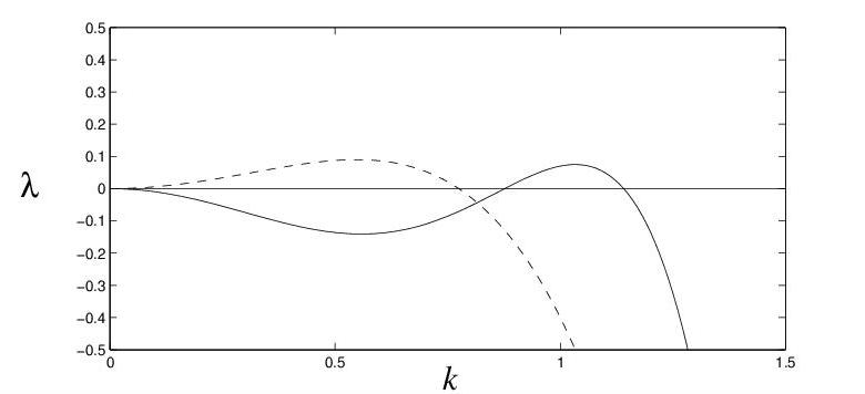
Figure 1: Curves illustrating two possible dispersion relations for front instabilities. Solid line: finite-wavenumber instability, leading to Nikolaevskiy equation (type I). Dashed line: long-wave instability, leading to Kuramoto–Sivashinsky equation (type II).

In either case, a nonlinear term must be added to the equation to limit the growth of the instability; its derivation is the same for either type of instability, and, as with the linear terms, only $x$-derivatives of $\phi$ may appear. The nonlinear term can be derived by a simple geometrical argument, considering the propagation of a tilted front kurbook . Such an argument leads to a nonlinear term which in our scaling takes the form $(\partial\phi/\partial x)^{2}/2$, as in (2) and (5).

We have shown that (2) may be regarded as a model equation for the transverse instability of a planar front at finite wavenumber. More generally, it is apparent that any physical system that gives rise to the Kuramoto–Sivashinsky equation might also lead to the Nikolaevskiy equation, depending on which of the two possible forms shown in Figure 1 is taken by the dispersion relation. Another example fy ; tan04 ; tk is the derivation of nonlinear phase equations; this leads to the Nikolaevskiy and Kuramoto–Sivashinsky equations, in different parameter regimes, as the dispersion relation changes from type I to type II. The argument in the case of phase equations is essentially identical to that given above for fronts, following from the invariance under addition of a constant to the phase, and under reflection in $x$.

There are many studies of the transverse linear stability of fronts in the literature, arising from a variety of different physical and chemical systems. A review of the literature reveals several examples of a finite-wavenumber (type I) instability, consistent with the Nikolaevskiy equation. For example, in their study of an evaporation front for condensed matter heated by a laser, Anisimov et al. ate found a linear spectrum of type I for transverse instability. Both types of instability were found in an experimental and theoretical study of a reaction front between two chemicals in a Hele-Shaw cell bansagi ; dhkdw ; kydw .

III The damped Nikolaevskiy equation

The complex chaotic behavior of the Nikolaevskiy equation at onset arises from the interaction between the unstable modes near $k=1$ and the neutral mode at $k=0$. However, in real physical systems it is likely that the symmetry giving rise to the neutral mode (such as translation or Galilean symmetry) will be weakly broken. For example, in the case of a propagating front, considered in Section II, the translation symmetry may be broken by the presence of boundaries, or by a slight variation in the basic state with position. With such a weak symmetry breaking, the $k=0$ mode will not be truly neutral, but will be weakly damped instead.

A further motivation for including a damping term in the Nikolaevskiy equation is that it allows us to study the transition from ordered stable patterns to soft turbulence. Such a probing of the origins of the turbulent state is not possible in the original Nikolaevskiy equation (1), since chaos is observed directly at onset (provided the domain is sufficiently large). Introduction of a damping term gives another parameter, which can be used to control and investigate the onset of chaos. A similar approach has been used to examine the dynamics of the Kuramoto–Sivashinsky equation brunet ; misbah .

We thus consider in this paper the “damped Nikolaevskiy” equation

$${\partial u\over\partial t}+u{\partial u\over\partial x}=-{\partial^{2}\over\partial x^{2}}\left(ru-\left(1+{\partial^{2}\over\partial x^{2}}\right)^{2}u\right)-\nu\left(1+{\partial^{2}\over\partial x^{2}}\right)^{2}u,$$ (6)

with damping coefficient $\nu\geq 0$; in particular we shall be concerned with the dynamics of (6) near the onset of pattern formation. In examining the stability of roll solutions, we shall find it useful to consider various cases for the relative sizes of the supercriticality parameter

$$r=\epsilon^{2}$$

and the damping coefficient $\nu$, and hence we write

$$\nu=\epsilon^{s}\mu,$$ (7)

where $\mu=O(1)$; we shall examine below a variety of pertinent values for $s$.

Of course there are many ways in which one might add damping to the Nikolaevskiy equation. The damping term in (6) is chosen so that all modes are linearly damped (with the exception of the mode with wavenumber $k=1$); large-scale modes decay at a rate $-\nu$. Furthermore, significant analytical simplifications follow from the fact that in (6) the onset of linear instability is independent of $\nu$ (i.e., the critical value of $r$ is $r_{c}=0$ and the critical wavenumber is $k_{c}=1$, for any $\nu\geq 0$). Note that our choice of damping term differs from that of Tribelsky try06 , who considers instead a damping term proportional to $-u-\partial^{2}u/\partial x^{2}$. Consequently, in his formulation both $r_{c}$ and $k_{c}$ become functions of $\nu$, leading to additional algebraic complications. However, the two formulations are equivalent under appropriate rescalings of $x$ and $t$, and appropriate mappings between the two parameter sets.

IV Secondary stability of rolls: numerical results

We begin our investigation of (6) by numerically computing spatially periodic steady “roll” solutions, and determining their secondary stability. To do so, first we fix $\epsilon$ and compute the roll solution $\bar{u}(x)$ for a given choice of $k$ and $\nu$ by integrating (6) forwards in time in a box of length $2\pi/k$. In our pseudospectral numerical code to achieve this, $\bar{u}$ is approximated by the truncated Fourier series

$$\bar{u}(x)=\sum_{-N}^{N}\bar{u}_{n}{\rm e}^{n{\rm i}kx}.$$

Disturbances $u^{\prime}(x)$ to this roll solution then satisfy, from (6),

$${\partial u^{\prime}\over\partial t}+u^{\prime}{\partial\bar{u}\over\partial x}+\bar{u}{\partial u^{\prime}\over\partial x}=-{\partial^{2}\over\partial x^{2}}\left(ru^{\prime}-\left(1+{\partial^{2}\over\partial x^{2}}\right)^{2}u^{\prime}\right)-\nu\left(1+{\partial^{2}\over\partial x^{2}}\right)^{2}u^{\prime},$$ (8)

and these disturbances are sought in the form

$$u^{\prime}(x)={\rm e}^{\sigma t+{\rm i}px}\sum_{-N}^{N}u_{n}^{\prime}{\rm e}^{n{\rm i}kx}$$ (9)

(where the sum is again truncated for numerical purposes). Equation (8) is thus reduced to a matrix eigenvalue problem for the growth rate $\sigma$. By computing $\sigma(p;k,\epsilon,\nu)$ for $p$ in the range $-k/2\leq p\leq k/2$, we are then able to determine the stability of the roll solution $\bar{u}(x)$.

(a)

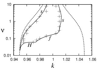
(b)

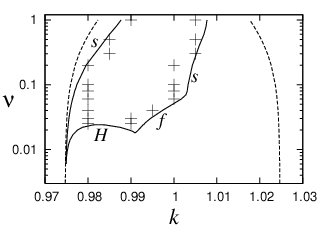
Figure 2: Stability boundaries of rolls in (6), computed numerically for (a) $\epsilon=0.1$ and (b) $\epsilon=0.05$. Rolls with wavenumber $k$ exist between the dashed curves, and are stable inside the region enclosed by solid curves. The annotations on the stability boundary indicate the type of instability suffered by the rolls upon crossing that part of the boundary: modulational steady (“s”), modulational Hopf (“H”) or finite-wavelength (“f”) instability. The crosses correspond to numerical simulations of the initial-value problem (6) in a large computational box and indicate the most extreme values of the wavenumber for which rolls are found to be stable to small perturbations (necessarily restricted to those that fit into the computational box); that all crosses lie inside the roll stability boundary provides a consistency check on our results.

Results for $\epsilon=0.1$ and $\epsilon=0.05$ are summarized in Figure 2, where rolls are stable inside the regions bounded by solid curves. For large enough damping (i.e., towards the top of each plot), the familiar Eckhaus stability boundaries are recovered. For sufficiently small damping, by contrast, all rolls are unstable – this shows that the known instability of all rolls in the undamped Nikolaevskiy equation extends to the case of (sufficiently small) finite damping, for a fixed value of the supercriticality parameter. Intermediate numerical results show the transition between the two limits.

Several features of Figure 2 merit comment. First, the region of stable rolls, which is roughly symmetrical about $k=1$ at large damping, becomes distinctly asymmetrical as the damping is reduced; rolls with $k>1$ tend to be less stable than those with $k<1$. Second, stability is finally lost, as $\nu$ is decreased, in a small cusp near the left-hand side of the marginal stability curve. For $\epsilon=0.1$, this corner is at $\nu\approx 0.02$ and $k\approx 0.950$ (the roll existence boundary is, for this value of $\nu$, at $k\approx 0.9493$); for $\epsilon=0.05$, we have found it much harder to compute the very thin cusp right down to its tip. The left and right sides of the cusp correspond, respectively, to monotonic and oscillatory long-wavelength instabilities. In fact the entire boundary corresponds to long-wavelength instabilities ($|p|\ll 1$), with the exception of the segment marked “f”, where the instability has finite wavelength ($p=O(1)$). For even smaller values of $\epsilon$ than shown in the figure, this finite-wavelength segment is absent, a point to which we shall return in Section V.3.1.

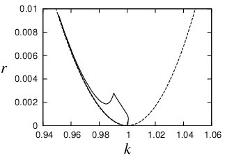
Figure 3: Stability boundaries of rolls in (6), computed numerically for $\nu=0.02$. Rolls with wavenumber $k$ exist between the dashed curves, and are stable inside the region enclosed by solid curves.

A more conventional picture of the stability balloon for rolls is shown in Figure 3, where the damping parameter $\nu$ is fixed to be $0.02$ and the stability of rolls is shown in the $(k,r)$-plane. Again rolls are stable inside the solid curves. The region of stable rolls lies almost entirely in the region $k<1$. For $r>0.003$, all rolls are unstable, except those exceedingly close to the left-hand part of the marginal stability curve; these rolls are last to lose stability as $r$ is increased. Finally, for $r>0.01$, all rolls are unstable. A corresponding picture for smaller damping coefficient $\nu$ would show stable rolls in a similar, but smaller region, confined closer to the point of onset ($r=0$, $k=1$). In the next section, we shall argue on the basis of asymptotic arguments that in the limit $\nu\to 0$ (approaching the undamped Nikolaevskiy equation), the size of the stable region shrinks to zero. Crucially, however, we expect a small, but finite, region of stable rolls in the $(k,r)$-plane for any nonzero value of the damping coefficient $\nu$. It is only for the undamped case $\nu=0$ that all rolls are unstable at onset.

V Secondary stability of rolls: analytical results

The numerical results in the previous section reveal a number of different instabilities of rolls in the damped Nikolaevskiy equation. In this section, we consider in detail three scalings for $\nu$ in (6) which shed particular light on the numerical stability results illustrated above: these correspond to choosing in turn $s=1$, $s=3/2$ and $s=2$ in (7).

V.1 Strong damping: $s=1$

The case $s=1$ represents strong damping, in the sense that the decay rate $\nu=\epsilon\mu$ of the large-scale mode is $O(\epsilon)$, which is much greater than the $O(\epsilon^{2})$ growth rate of the pattern-forming mode. The effect of this strong damping is simply to modify the usual Ginzburg–Landau amplitude equation and thus modify the Eckhaus stability boundary, as we now demonstrate. Our conclusions below are consistent with those obtained by Tribelsky try06 , although his analysis proceeds directly from a substitution of (9) into (8), rather than the amplitude-equation framework developed below.

We apply to (6) the usual weakly nonlinear scalings and expand the solution as

$$u=\epsilon(A(X,T){\rm e}^{{\rm i}x}+{\rm c.c.})+\epsilon^{2}u_{2}+\epsilon^{3}u_{3}+\cdots,$$ (10)

where $X=\epsilon x$ and $T=\epsilon^{2}t$, and where c.c. denotes the complex conjugate of the preceding term. At $O(\epsilon)$, (6) is satisfied. At $O(\epsilon^{2})$, we find

$$u_{2}=(-{\textstyle\frac{1}{36}}{\rm i}A^{2}{\rm e}^{2{\rm i}x}+{\rm c.c.})+f(X,T),$$

where the large-scale mode $f(X,T)$ is arbitrary. At $O(\epsilon^{3})$, an equation arises for the mean mode $f$, which represents a balance between the driving term $(|A|^{2})_{X}$ and the damping term $-\mu f$:

$$0=-(|A|^{2})_{X}-\mu f.$$ (11)

Note that the linear terms $f_{T}$ and $f_{XX}$ do not appear at this order. The governing equation for $A$ is also obtained at $O(\epsilon^{3})$, by applying the usual solvability condition. It turns out to be

$$A_{T}=A+4A_{XX}-{\textstyle\frac{1}{36}}|A|^{2}A-{\rm i}fA,$$ (12)

from which $f$ may be eliminated using (11) to give a single amplitude equation for $A$ in the form

$$A_{T}=A+4A_{XX}-{\textstyle\frac{1}{36}}|A|^{2}A+{\rm i}(|A|^{2})_{X}A/\mu.$$ (13)

This is the usual Ginzburg–Landau equation for $A$, but with an additional nonlinear derivative term arising from the damping. Extensions to the Ginzburg–Landau equation including terms such as ${\rm i}(|A|^{2})_{X}A$ are well known doe ; hoy , but the different scalings involved here have the consequence that no further terms need be included to ensure that all terms of a given asymptotic order are present: with our scalings, (13) is complete. Note that in the limit $\mu\to\infty$, we recover the usual Ginzburg–Landau equation for $A$.

It is straightforward to analyse the stability of patterns in (13) – see Mancebo and Vega man . Steady patterns with $A=a_{0}\exp{{\rm i}qX}$ exist for $q^{2}<q_{c}^{2}=1/4$, with the real amplitude $a_{0}=6(1-4q^{2})^{1/2}$. The stability of these solutions may be determined by writing $A=(a_{0}+a(X,T))\exp{{\rm i}qX}$ and linearizing in the perturbation $a$, to give

$$a_{T}=-{\textstyle\frac{1}{36}}a_{0}^{2}(a+a^{*})+8{\rm i}qa_{X}+4a_{XX}+{\rm i}a_{0}^{2}(a_{X}+a^{*}_{X})/\mu.$$ (14)

After writing $a=b+{\rm i}c$, and separating (14) into real and imaginary parts, we find that $b$ and $c$ obey

$$b_{T} = -{\textstyle\frac{1}{18}}a_{0}^{2}b-8qc_{X}+4b_{XX},$$ (15)

$$c_{T} = 8qb_{X}+4c_{XX}+2a_{0}^{2}b_{X}/\mu.$$ (16)

Then by supposing $b$ and $c$ each to be proportional to $\exp({\lambda T+{\rm i}lX})$, we find that the growth rate $\lambda$ satisfies

$$\lambda^{2}+({\textstyle\frac{1}{18}}a_{0}^{2}+8l^{2})\lambda+16l^{4}+{\textstyle\frac{2}{9}}a_{0}^{2}l^{2}-64q^{2}l^{2}-16ql^{2}a_{0}^{2}/\mu=0;$$ (17)

only monotonic instability is possible, and there can be instability if and only if

$$l^{2}(72l^{2}+a_{0}^{2}-288q^{2}-72qa_{0}^{2}/\mu)<0.$$ (18)

It is clear from (18) that the most “dangerous” modes are those with small $l$, so the pattern is stable if

$$(1-12q^{2})>72q(1-4q^{2})/\mu.$$ (19)

The corresponding stability boundaries are shown in Figure 4.

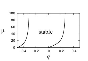
Figure 4: Stability boundaries of rolls according to (19), in $(q,\mu)$-space, where the damping coefficient $\nu=\epsilon\mu$. Rolls exist for $-1/2<q<1/2$ and are stable in the region between the two curves, where indicated. In the limit $\mu\to 0$, the stable rolls are those with $q<0$. In the limit as $\mu\to\infty$, the usual Eckhaus stability boundary is recovered, so that rolls are stable for $-(1/12)^{1/2}<q<(1/12)^{1/2}$.

In the limit $\mu\to\infty$, the usual Eckhaus stability condition (that rolls are stable for $q^{2}<q_{e}^{2}\equiv{\textstyle\frac{1}{3}}q_{c}^{2}={\textstyle\frac{1}{12}}$) is recovered from (19). As $\mu$ is decreased, however, an asymmetry develops in the stability region: patterns are stable for $f(\mu)<q<g(\mu)$, where $f(\mu)\in[-{\textstyle\frac{1}{2}},-q_{e})$ and $g(\mu)\in[0,q_{e})$ are each increasing functions of $\mu$. When $\mu$ is small, the stability condition is roughly $q(1-4q^{2})<0$, so that patterns with $q>0$ are unstable and patterns with $q<0$ are stable. A corresponding conclusion is reached by Tribelsky (whose results are plotted in his Figure 1(a)). If we compare the results of this analysis with the numerical stability calculations described above in Section IV, we see that the stability boundaries in Figure 4 correspond, roughly, to those in Figure 2 above $\nu\approx 0.2$ (for $\epsilon=0.1$) and above $\nu\approx 0.07$ (for $\epsilon=0.05$).

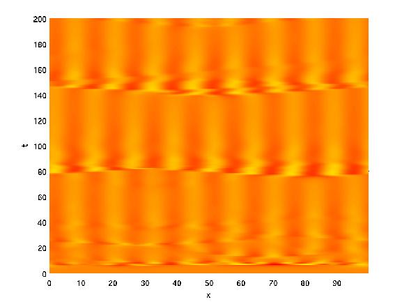
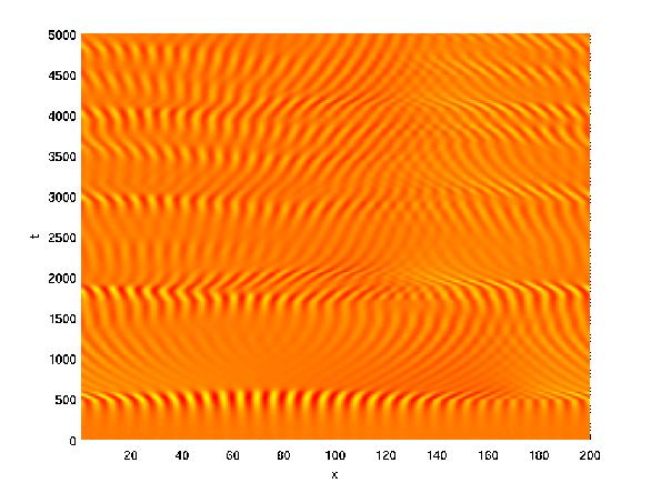
Figure 5: Space–time plots of numerical solutions of (13), for $\mu=0.1$ (left, real part of $A$ plotted), and the undamped Nikolaevskiy equation (1) with $r=0.01$ (right).

The above analysis shows that for small $\mu$, patterns with $q<0$ are stable in (13). However, numerical simulations of (13) in a periodic domain, started from a random, small amplitude initial condition do not always lead to stable patterns. A typical simulation, for $\mu=0.1$, in a domain of size 100, is shown in Figure 5 (left). The solution is dominated by a state with 8 rolls in the domain, with a wavenumber $q=-8\times 2\pi/100\approx-0.5026$, which is just outside the range of wavenumbers for which steady patterns exist. This mode must therefore decay, until a bursting event occurs, involving other wavenumbers, from which the 8-roll state again emerges. Simulations with different domain sizes show that (13) seems to exhibit a preference for modes near to the left-hand limit of the region of existence of steady states, $q=-1/2$. Note that this behavior is shared by the damped Nikolaevskiy equation (6), as shown in Figure 2. Another qualitative similarity between the behavior of (13) and the Nikolaevskiy equation is that both exhibit irregular bursting behavior (albeit with rather different detailed structures). For comparison, a simulation of the undamped Nikolaevskiy equation (1) in a domain of size 200, for $r=0.01$, is shown in Figure 5 (right).

In the limit $\mu\to 0$, it is clear from (17) that the eigenvalues $\lambda$ become large, of order $\mu^{-1/2}$. This indicates that a different scaling is required in which the damping $\nu$ is smaller than $O(\epsilon)$ and the growth rate of the instability is greater than $O(\epsilon^{2})$; this next scaling is considered in the following section.

V.2 Intermediate damping: $s=3/2$

The analysis above corresponds to damping that is sufficiently strong to enslave the large-scale mode to gradients of the pattern amplitude. More subtle effects of damping can be explored if it is rather weaker: if $s=3/2$ in (6). Our starting point is now the general roll solution of (6) with $\nu=\epsilon^{3/2}\mu$, which may be written in the form

$$u=\epsilon a_{0}{\rm e}^{(1+\epsilon q){\rm i}x}+\mbox{c.c.}+O(\epsilon^{2}),$$

where $a_{0}=6(1-4q^{2})^{1/2}$.

A proper treatment of the stability of rolls requires consideration of the evolution of both amplitude and phase of the rolls, together with a large-scale mode. All three modes couple together, and their relative scalings, together with appropriate length and time scales for their evolution, are chosen below to enable a balance in the linearized perturbation problem; this is essentially the balance considered in mat . However, by making appropriate absolute scalings for the three perturbation quantities, we are able to extend the linear results in mat and accommodate the first nonlinear term in the evolution equations that follow. We shall see below that this enables us to describe the sub- or supercritical nature of the onset of instability of the rolls. It turns out that the appropriate scaling for the three perturbation quantities is accomplished by writing

$$u=\epsilon(a_{0}+\epsilon^{1/2}a(X,T)){\rm e}^{{\rm i}x}{\rm e}^{{\rm i}q\epsilon x}{\rm e}^{{\rm i}\epsilon^{1/4}\phi(X,T)}+\mbox{c.c.}+\cdots+\epsilon^{7/4}f(X,T)+\cdots,$$ (20)

where now

$$X=\epsilon^{3/4}x,\qquad T=\epsilon^{3/2}t.$$

Note that in order to simplify notation we use the same symbols ($X$ and $T$) in different sections to represent different length and time scales. Notation within any one section is consistent, so no confusion should arise.

Then after a systematic substitution of (20) in (6) and a consideration of terms at successive powers of $\epsilon^{1/4}$ we eventually find

$${\partial\phi\over\partial T} = 4{\partial^{2}\phi\over\partial X^{2}}-f,$$ (21)

$${\partial f\over\partial T} = {\partial^{2}f\over\partial X^{2}}-\mu f-2a_{0}{\partial a\over\partial X},$$ (22)

$${\partial a\over\partial T} = 4{\partial^{2}a\over\partial X^{2}}-4a_{0}\left({\partial\phi\over\partial X}\right)^{2}-8qa_{0}{\partial\phi\over\partial X}.$$ (23)

The linear terms in this equation may be identified with the linear system considered in mat , with the addition here of the new damping term $-\mu f$ in (22) (the quantities $b$, $c$ and $f$ in mat correspond, respectively, to our $a$, $a_{0}\phi$ and $f$); the nonlinear term was not computed in mat . These three equations may then be reduced to the nonlinear phase equation

$$\left({\partial\over\partial T}-4{\partial^{2}\over\partial X^{2}}\right)^{2}\left({\partial\over\partial T}-{\partial^{2}\over\partial X^{2}}+\mu\right)\phi=-16a_{0}^{2}\left(q+{\partial\phi\over\partial X}\right){\partial^{2}\phi\over\partial X^{2}}.$$ (24)

In analysing (24), it is useful to consider first the linearized problem, for which the right-hand side is simply $-16a_{0}^{2}q\phi_{XX}$. This term represents the coupling between $\phi$, $a$ and $f$: in its absence, no instability can result in (24). Thus in Sections V.2.1 and V.2.2 below we assume $a_{0}^{2}q=O(1)$. However, we should note that the analysis described below must be reconsidered when $|a_{0}^{2}q|$ is small (cf. triv ) – we see immediately that there are two circumstances in which a separate consideration is warranted ($a_{0}\ll 1$ and $|q|\ll 1$); we shall return to this important point below, in Section V.3.

V.2.1 No damping

We begin by summarizing relevant results in the absence of damping. When $\mu=0$ we recover from (24) the secondary stability results obtained by Tribelsky and Velarde triv and elsewhere by ourselves mat : there is monotonic instability of the rolls with $q>0$, and such rolls are unstable to disturbances with wavenumbers $l$ in the range $0<|l|<l_{cm}\equiv(a_{0}^{2}q)^{1/4}$; there is oscillatory instability for $q<0$, and here the instability strikes for $0<|l|<l_{co}\equiv(-2a_{0}^{2}q/25)^{1/4}$. Thus all rolls are unstable at onset in the undamped problem.

It is instructive to extend the linearized analysis by considering the weakly nonlinear development of these instabilities, according to (24). We shall focus on computing the coefficients of the nonlinear terms in Landau equations for the amplitudes of the disturbances; the signs of the real parts of these coefficients will indicate the direction of bifurcation to the perturbed state. We consider first the monotonic instability for $q>0$, and examine the evolution of a disturbance whose wavenumber satisfies $|l-l_{cm}|=O(\delta)$, where $0<\delta\ll 1$. Expanding

$$\phi=\delta\phi_{1}+\delta^{2}\phi_{2}+\cdots,$$ (25)

where

$$\phi_{1}=A(T_{2})\sin lX$$

and $T_{2}=\delta^{2}T$, we find at $O(\delta^{3})$ that

$${\frac{{\rm d}A}{{\rm d}T_{2}}}=\frac{a_{0}^{2}}{180q}A^{3}.$$

Thus the bifurcation is always subcritical and hence leads to the observed explosive growth of the instability in simulations of the undamped Nikolaevskiy equation mat ; triv . For the oscillatory instability for $q<0$, we instead suppose that $|l-l_{co}|=O(\delta)$; again expanding $\phi$ as in (25), but now with

$$\phi_{1}={\rm e}^{{\rm i}\omega T}\left(B(T_{2}){\rm e}^{{\rm i}lX}+C(T_{2}){\rm e}^{-{\rm i}lX}\right)+\mbox{c.c.},$$

where $\omega=(-48a_{0}^{2}q/25)^{1/2}$, we find at $O(\delta^{3})$ the Landau equations

$$\frac{-q}{a_{0}^{2}B}{\frac{{\rm d}B}{{\rm d}T_{2}}} = \left(-\frac{740}{72639}+\frac{55\sqrt{6}}{8071}{\rm i}\right)|B|^{2}+\left(-\frac{40}{1197}-\frac{10\sqrt{6}}{399}{\rm i}\right)|C|^{2},$$ (26)

$$\frac{-q}{a_{0}^{2}C}{\frac{{\rm d}C}{{\rm d}T_{2}}} = \left(-\frac{740}{72639}+\frac{55\sqrt{6}}{8071}{\rm i}\right)|C|^{2}+\left(-\frac{40}{1197}-\frac{10\sqrt{6}}{399}{\rm i}\right)|B|^{2}.$$ (27)

Since $q<0$, both travelling waves and standing waves branch supercritically, with the travelling wave stable. In practice we expect the explosive development of the monotonic instability to dominate the smooth onset of the oscillatory instability in simulations of the undamped Nikolaevskiy equation, except under extremely controlled (and contrived) conditions.

V.2.2 Nonzero damping

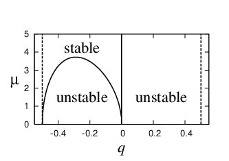
Figure 6: Stability boundaries of rolls, based on analysis of the case of intermediate damping, $\nu=\epsilon^{3/2}\mu$. Rolls exist between the dashed lines and are stable or unstable as indicated. The solid vertical straight line represents the onset of a monotonic bifurcation and the solid curve represent a Hopf bifurcation.

For $\mu>0$, we again begin by examining the linearized behavior of (24). A monotonic instability again occurs for all rolls with $q>0$, with the stability margin being given by $l_{cm}^{4}+\mu l_{cm}^{2}-qa_{0}^{2}=0$. It thus follows that

$$l^{4}_{cm}(\mu)=qa_{0}^{2}-\mu l_{cm}^{2}<qa_{0}^{2}=l^{4}_{cm}(0),$$

and hence the rolls are unstable to a smaller range of disturbance wavenumbers than in the undamped case. An oscillatory instability arises for rolls with $q<q_{0}$, where $q_{0}=-\mu^{2}/(2a_{0}^{2})$; such rolls are unstable to disturbances with $0<|l|<l_{co}$, where now $5l_{co}^{2}=-\mu+(-2qa_{0}^{2})^{1/2}$. We may rewrite the condition $q<q_{0}$ for instability as

$$72q(1-4q^{2})<-\mu^{2}.$$ (28)

Then since the cubic function in (28) has a minimum value of $-8\sqrt{3}$ at $q=-\sqrt{3}/6$, this oscillatory instability can occur only for $\mu^{2}<8\sqrt{3}$, that is, for sufficiently weak damping (this is consistent with no oscillatory instability being observed in the previous scaling of stronger damping in Section V.1). In the limit of small $\mu$ the stability boundaries in (28) approach $q=0$ and $q=-1/2$, so that all rolls with $q<0$ are predicted to be unstable to an oscillatory disturbance, just as in the undamped case.

The stability boundaries for this scaling are illustrated in Figure 6. Note that the curved line of the Hopf bifurcation is consistent with the numerical stability results for the full damped Nikolaevskiy equation (6) shown in Figure 2 (except, of course, that the analysis above does not capture the finite-wavelength instability denoted by “f” in Figure 2). Figure 6 suggests that two regions of stable rolls, near $q=0$ and $q=-1/2$, extend right down to zero damping. But in each of these cusped regions, $|a_{0}^{2}q|=|6q(1-4q^{2})^{1/2}|\ll 1$, and we recall that the present scaling is not valid in this limit. Thus we should disregard the two cusps in Figure 6 at small damping and instead examine more closely the stability of rolls in this limit; to resolve the correct behavior of the stability boundary at small damping, we consider in the next section a further (and final) scaling for $\nu$.

V.3 Weak damping: $s=2$

The final small-$\epsilon$ asymptotic description of the roll stability boundary may be described by setting $s=2$, so that $\nu=\epsilon^{2}\mu$. In this case, the damping rate of the mean mode is of the same order as the growth rate of the pattern-forming mode. There are two cases to consider where the scaling of the previous section breaks down, corresponding to $|q|\ll 1$ and $a_{0}\ll 1$.

V.3.1 Central corner ($|q|\ll 1$)

As Tribelsky and Velarde triv have pointed out for the case of no damping, the scalings of Section V.2 break down when $q$ is small. To resolve the small-$q$ behavior, we adopt Tribelsky and Velarde’s scalings (but in an amplitude-equation framework) and consider

$$u\sim\epsilon(a_{0}+\epsilon^{2}a(X,T)){\rm e}^{{\rm i}x}{\rm e}^{{\rm i}\epsilon^{2}qx}{\rm e}^{{\rm i}\epsilon\phi(X,T)}+\mbox{c.c.}+\cdots+\epsilon^{3}f(X,T)+\cdots,$$ (29)

where now $X=\epsilon x$ and $T=\epsilon^{2}t$ and $a_{0}=6$. Note that whereas (20) concerns basic roll wavenumbers $k=1+O(\epsilon)$, (29), by contrast, concerns the much narrow wavenumber band $k=1+O(\epsilon^{2})$. We find, after a substitution of (29) in (6),

$${\partial\phi\over\partial T} = 4{\partial^{2}\phi\over\partial X^{2}}-f,$$ (30)

$${\partial f\over\partial T} = {\partial^{2}f\over\partial X^{2}}-\mu f-2a_{0}{\partial a\over\partial X},$$ (31)

$${\partial a\over\partial T} = 4{\partial^{2}a\over\partial X^{2}}-\frac{1}{18}a_{0}^{2}a+a_{0}\left(\frac{11}{54}a_{0}^{2}-8q+12{\partial^{2}\over\partial X^{2}}\right){\partial\phi\over\partial X}-4a_{0}\left({\partial\phi\over\partial X}\right)^{2}-a_{0}{\partial f\over\partial X}.$$ (32)

These three equations may then be reduced to the single nonlinear phase equation

$$\left({\partial\over\partial T}-4{\partial^{2}\over\partial X^{2}}\right)\left({\partial\over\partial T}-4{\partial^{2}\over\partial X^{2}}+\frac{1}{18}a_{0}^{2}\right)\left({\partial\over\partial T}-{\partial^{2}\over\partial X^{2}}+\mu\right)\phi=$$

$$2a_{0}^{2}\left(\frac{11}{54}a_{0}^{2}-8q+{\partial\over\partial T}+8{\partial^{2}\over\partial X^{2}}\right){\partial^{2}\phi\over\partial X^{2}}-16a_{0}^{2}{\partial\phi\over\partial X}{\partial^{2}\phi\over\partial X^{2}}.$$ (33)

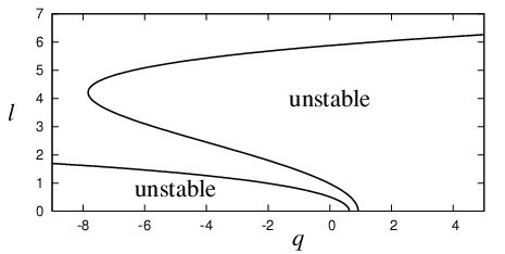
Figure 7: Stability boundaries of small-$q$ rolls, according to (33), in the undamped case $\mu=0$ (cf. triv ). To the right is the monotonic stability boundary for rolls; to the left is the oscillatory stability boundary.

We now consider the linearized version of (33) and examine the dispersion relation for infinitesimal disturbances proportional to $\exp(\sigma T+{\rm i}lX)$. It is helpful first to recall the stability results of Tribelsky and Velarde triv for the case $\mu=0$, which are summarized in Figure 7, and which are a special case of the more general analysis to be presented below. As can be seen in the figure, all rolls are unstable for $\mu=0$.

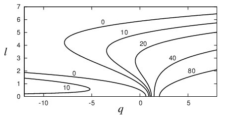
Figure 8: Stability boundaries of rolls with damping coefficient $\nu=\epsilon^{2}\mu$, according to (33), for values of $\mu$ as indicated. To the right are the monotonic stability boundaries; to the left are the oscillatory stability boundaries. As the damping coefficient increases, the rolls become less unstable. For sufficiently large $\mu$, a stable band of wavenumbers emerges.

For general values of $\mu$, rolls undergo a monotonic instability ($\sigma=0$) when $q=q_{m}(l,\mu)$, where

$$72q_{m}(l,\mu)=2l^{4}+(2\mu-71)l^{2}+66+\mu.$$

Since $q_{m}(l,\mu)>q_{m}(l,0)$, it follows that the stability margin tends to move to the right as the damping is increased, tending to stabilize the rolls (see Figure 8). Rolls undergo an oscillatory instability ($\sigma={\rm i}\omega$) when

$$q=-\frac{\mu(2+\mu)}{288}l^{-2}-\left(\frac{\mu^{2}}{72}+\frac{3\mu}{16}-\frac{91}{144}\right)-\left(\frac{5\mu}{36}+\frac{677}{288}\right)l^{2}-\frac{25}{72}l^{4},$$ (34)

with onset frequency given by

$$\omega^{2}=24l^{4}+2(4\mu+41)l^{2}+2\mu.$$

The oscillatory stability boundary is plotted in Figure 8 for various values of $\mu$. Damping is seen to shift the oscillatory stability curve to the left, again stabilizing the rolls. A further effect of nonzero damping is to stabilize rolls to oscillatory disturbances in the limit that the perturbation wavenumber $l\to 0$.

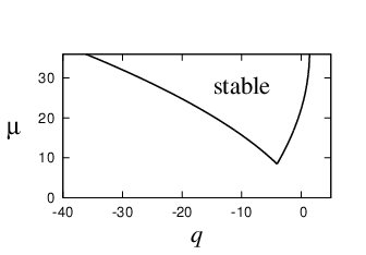
Figure 9: Stability boundary for rolls with wavenumber $1+\epsilon^{2}q$, according to (33), for weak damping, with $\nu=\epsilon^{2}\mu$. Rolls are stable inside the wedge. At the right-hand boundary they become susceptible to a monotonic instability, at the left-hand boundary an oscillatory instability. The wedge terminates at the point $(\mu,q)\approx(8.445,-4.049)$.

As can be seen from Figure 8, with increasing damping the two stability boundaries separate and eventually part, allowing a small band of stable rolls. We find that stable rolls exist for $\mu>\mu_{c}\approx 8.445$ (the corresponding critical value of $\nu$ is $\nu_{c}=\mu_{c}\epsilon^{2}$); thus, for a given value of the supercriticality parameter, there is a threshold value of the damping coefficient to allow stable rolls near $k=k_{c}$, as previously shown by Tribelsky try06 . Figure 9 shows the region of stable rolls in $(\mu,q)$-space (thus the apparent small-$q$ cusp in Figure 6, which appears to extend down to zero damping, is in fact a wedge terminating at finite damping).

The results above seem at odds with the numerical results presented in Figure 2, since there is no central wedge in the numerical stability boundary. However, it turns out that for the values of $\epsilon$ used in Figure 2, the small-$q$ wedge is masked by an additional finite-wavenumber instability. For a smaller value of $\epsilon$, the theory in this section does indeed correctly predict the shape of the stability boundary, as shown in Figure 10 for $\epsilon=0.01$. (It becomes increasingly challenging to compute the entire stability boundary numerically, so only the relevant part is presented for this value of $\epsilon$.) Rolls are stable in the wedge down to $\nu\approx 8.445\epsilon^{2}$, and the last rolls to destabilize have wavenumber approximately $1-4.049\epsilon^{2}$. These results agree with corresponding results of Tribelsky try06 .

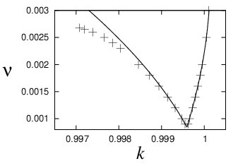
Figure 10: Stability boundary for rolls in (6), computed numerically for $\epsilon=0.01$, near the central wedge region corresponding to Figure 9. Crosses indicate numerical results and the solid line corresponds to our analytical results (cf. Figure 9). Note that for this value of $\epsilon$ (and presumably also for even smaller values) the numerical stability boundary contains this central wedge rather than a section corresponding to that marked “f” in Figure 2.

V.3.2 Left-hand corner ($a_{0}\ll 1$)

We now examine the second case in which the asymptotic results of Section V.2 break down: $a_{0}\ll 1$. This regime proves to include the last rolls to become destabilized as the damping is reduced. We thus investigate the stability of rolls close to the marginal stability boundary. Recall from Section V.2 and in particular Figure 6 that we expect stable rolls to persist to small values of the damping near the left-hand side of the marginal stability curve.

We introduce the notation $k=k_{m}^{-},k_{m}^{+}$ for the left- and right-hand marginal stability boundaries, respectively (that is, for given values of $r$ and $\nu$, rolls exist for wavenumbers $k$ in the range $k_{m}^{-}<k<k_{m}^{+}$). We shall begin by considering both left- and right-hand parts of the marginal stability curve, since both lead to $a_{0}\ll 1$. Our analysis will then show that only the left-hand part of the marginal curve is relevant, being capable of supporting stable rolls. We find, from substitution in the equation $k_{m}^{2}[\epsilon^{2}-(1-k_{m}^{2})^{2}]-\epsilon^{2}\mu(1-k_{m}^{2})^{2}=0$ for the marginal curve, that

$$k_{m}^{\pm}=1\pm{\textstyle\frac{1}{2}}\epsilon-{\textstyle\frac{1}{8}}\epsilon^{2}\pm({\textstyle\frac{1}{16}}-{\textstyle\frac{1}{4}}\mu)\epsilon^{3}+\cdots.$$

It turns out that the correct scaling to resolve the stability boundary of the rolls is obtained by setting $|k-k_{m}^{\pm}|=O(\epsilon^{2})$, in which case $|\bar{u}|=O(\epsilon^{3/2})$, with the relevant space and time scales for the evolution of perturbations being $X=\epsilon x$ and $T=\epsilon^{2}t$. We consider here only the linearized secondary stability problem and we are thus at liberty to scale arbitrarily the absolute sizes of the three perturbation quantities, keeping their relative sizes fixed. Thus we suppose that

$$u\sim\epsilon^{3/2}(a_{0}+a(X,T)){\rm e}^{{\rm i}kx}{\rm e}^{{\rm i}\phi(X,T)}+\mbox{c.c.}+\cdots+\epsilon^{2}f(X,T)+\cdots,$$ (35)

where the wavenumber of the rolls under consideration is just inside the marginal curve, so that

$$k=k_{m}^{\pm}\mp\epsilon^{2}\kappa.$$

A weakly nonlinear calculation of the roll solution itself shows that the amplitude and wavenumber are related by

$$a_{0}^{2}=144\kappa.$$ (36)

Then a consideration of the terms in (6) which are linear in the perturbation quantities $\phi$, $a$ and $f$ shows that their evolution is governed by

$$a_{0}{\partial\phi\over\partial T} = 4a_{0}{\partial^{2}\phi\over\partial X^{2}}-a_{0}f\pm 4{\partial a\over\partial X},$$ (37)

$${\partial f\over\partial T} = {\partial^{2}f\over\partial X^{2}}-\mu f-2a_{0}{\partial a\over\partial X},$$ (38)

$${\partial a\over\partial T} = 4{\partial^{2}a\over\partial X^{2}}\mp 4a_{0}{\partial\phi\over\partial X}.$$ (39)

These three equations may then be combined to yield a single linearized phase equation in the form

$$\left({\partial\over\partial T}-{\partial^{2}\over\partial X^{2}}+\mu\right)\left[\left({\partial\over\partial T}-4{\partial^{2}\over\partial X^{2}}\right)^{2}+16{\partial^{2}\over\partial X^{2}}\right]\phi=\mp 8a_{0}^{2}{\partial^{2}\phi\over\partial X^{2}}.$$ (40)

For modes proportional to $\exp(\sigma T+{\rm i}lX)$, this gives the dispersion relation

$$\left(\sigma+l^{2}+\mu\right)\left[\left(\sigma+4l^{2}\right)^{2}-16l^{2}\right]=\pm 8a_{0}^{2}l^{2}.$$ (41)

In the limit $a_{0}\to 0$, (41) gives the growth rates $\sigma=-(\mu+l^{2})<0$, $\sigma=4l(1-l)$ and $\sigma=4l(-1-l)$, and hence all rolls are unstable (to a monotonic disturbance) sufficiently close to the marginal curve. We gain some insight into the possible existence of stable rolls near the marginal curve by next considering the limit of small perturbation wavenumbers, $l\to 0$. For fixed $a_{0}$ and $\mu$, in the limit $l\to 0$, the leading-order balance in (41) is

$$\sigma^{2}\sim 8l^{2}(2\pm a_{0}^{2}/\mu).$$ (42)

Thus near $k=k_{m}^{+}$ rolls are unstable, to monotonic disturbances, since $(2+a_{0}^{2}/\mu)>0$. No further analysis of this case is necessary: there is no pocket of stable rolls possible near the right-hand marginal stability curve; this conclusion is consistent with Figure 2.

Near $k=k_{m}^{-}$, by contrast, the conclusion of monotonic instability follows from (42) only if $a_{0}^{2}<2\mu$ (i.e., sufficiently close to the marginal curve). When $a_{0}^{2}>2\mu$, (42) instead indicates oscillations, and we must go further in our consideration of the small-$l$ problem in order to determine the stability of the rolls. By carrying out a small-$l$ expansion of the growth rate in the form $\sigma=\sigma_{1}l+\sigma_{2}l^{2}+\cdots$, we find from (41) that $\sigma_{1}^{2}=8(2-a_{0}^{2}/\mu)$ and $\sigma_{2}=4(a_{0}^{2}/\mu^{2}-1)$. Thus when

$$2\mu<a_{0}^{2}<\mu^{2},$$ (43)

rolls are stable in the small-$l$ limit (the lower threshold for $a_{0}^{2}$ corresponding to a monotonic instability, the upper threshold to an oscillatory instability). The relation (43) indicates that rolls enjoy this region of stability only for sufficiently large damping: $\mu>\mu_{c}\equiv 2$. Note that since $2<8.445$ this cusp contains the last stable rolls as the damping is decreased.

In terms of the original variables in the damped Nikolaevskiy equation (6), we thus predict (for small $\nu$) the cusp to be at $\nu\sim 2r=2\epsilon^{2}$. We may readily check these analytical results against the numerical secondary stability calculations of Section IV. For $\epsilon=0.1$, as in Figure 2, we thus predict the apex of the cusp to lie at $\nu=0.02$ (which we do indeed find numerically). Similarly, for $\epsilon=0.05$ we predict the apex to lie at $\nu=0.005$, and the smallest value of $\nu$ for which we have been able to compute the cusp is $\nu=0.006$, which provides reasonable agreement with the theory. (As $\epsilon\to 0$ it becomes exceedingly difficult to compute accurately this part of the numerical secondary stability boundary.)

For completeness, we note that we have also considered numerically the full dispersion relation (41) for arbitrary values of $l$: we find that (at least for values of $a_{0}$ and $\mu$ up to $4$, for which we have carried out calculations) the stability boundary is indeed determined by the small-$l$ expansion.

VI Numerical simulations

In this section we present full numerical simulations of the damped Nikolaevskiy equation (6), illustrating the transition from regular patterns to soft-mode turbulence as the damping is reduced. The simulations use periodic boundary conditions and employ a Fourier spectral method for the spatial discretization. The time-stepping is an explicit second-order Runge–Kutta form of the exponential time differencing method cm02 that computes the stiff linear part of the equation exactly, permitting $O(1)$ time steps. The size of the domain is $200\pi$, allowing a resolution of $0.01$ in wavenumber.

In the simulations shown in Figure 11, the initial condition comprises rolls with wavenumber $k=0.96$, plus a small random perturbation. In each case, the simulation was run for a long time to remove transient features, and then plotted over a subsequent relatively short time interval. Note that these time intervals are not the same in each case. The driving parameter was fixed at $r=0.01$ and the sequence of simulations shows the effect of reducing $\nu$. For these parameters, all rolls that fit into the computational domain are predicted to be unstable for $\nu<\nu_{c}$ where $\nu_{c}\approx 0.057$. The bifurcation at $\nu=\nu_{c}$ is the Hopf bifurcation whose stability boundary is shown in Figures 2 and 6.

The simulations confirm the predicted bifurcation type, since for $\nu<\nu_{c}$ a small oscillatory modulation to the rolls grows. This bifurcation seems to be supercritical since the oscillations equilibrate to a small periodic modulation of the rolls. For $\nu=0.04$ this oscillation takes the form of a standing wave, as shown in Figure 11 (top). At $\nu=0.03$, the solution is no longer periodic in time and shows occasional irregular bursts of instability. In this case, the dominant wavenumber is $k=0.95$, at the left-hand boundary of the roll-existence region (i.e., near $k=k_{m}^{-}$), consistent with the analysis of the preceding section and the behavior of (13). Also, counter-intuitively, the amplitude of the solution becomes significantly lower as the damping is decreased. This is because of the transition from the $O(\epsilon)$ scaling in the strongly damped case to the $O(\epsilon^{3/2})$ scaling mat in the undamped, unstable regime. For $\nu=0.02$, the bursts are more frequent and a broad spectrum of wavenumbers is present in the solution. Finally, the lowest panel of Figure 11 shows the case of zero damping. This is significantly different from the weakly damped case, showing grain boundaries between regions of travelling rolls.

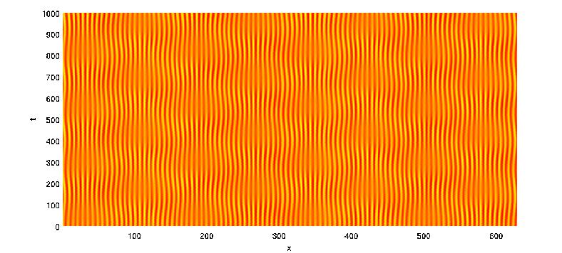
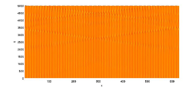
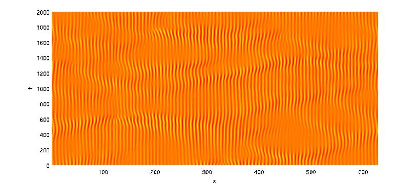
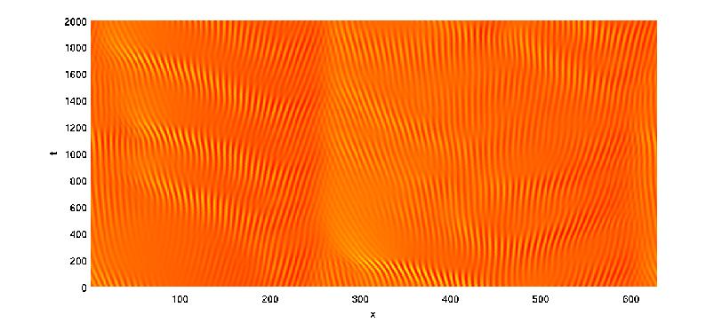
Figure 11: Space–time plots of the numerical solution of (6) at $r=0.01$. Top to bottom: $\nu=0.04$, $0.03$, $0.02$, $0$.

VII Discussion and conclusions

The Nikolaevskiy equation is an important model of a wide range of physical systems, including certain convection problems, phase instabilities and transverse instabilities of fronts. It arises naturally in systems with a finite-wavenumber instability and a translation symmetry for the dependent variable. However, in many applications it is likely that this symmetry will be weakly broken.

The damped Nikolaevskiy equation (6) allows us to investigate the effects of weak symmetry breaking, and describe the transition between the appearance of soft-mode turbulence at onset when $\nu=0$ and the more gradual development of complex dynamics typical of damped systems when the damping coefficient $\nu>0$. Our numerical investigation of the secondary stability problem for steady roll solutions shows how the instability of all roll states in the undamped case evolves into the more common Eckhaus scenario, whereby rolls with wavenumbers sufficiently close to critical are stable, when the damping is sufficiently great. If we fix the supercriticality parameter $r$, then it follows from the asymptotic results of Section V.3.2 that there is a critical value of the damping coefficient $\nu=\nu_{c}$ (given by $\nu_{c}\sim 2r$ when $r$ is small) below which all rolls are unstable; for $\nu>\nu_{c}$ some rolls are stable.

However, it is more common in applications to fix parameters such as the damping coefficient $\nu$ and vary the supercriticality parameter $r$. Then the results of Section V.3.2 may be interpreted as indicating that, at least for small values of $\nu$, there are stable rolls provided $2r<\nu$, i.e., close enough to onset. Thus the damped Nikolaevskiy equation differs fundamentally from the undamped version in that there is not a direct transition to soft-mode turbulence at onset when $\nu>0$; instead, there is a sequence of bifurcations beginning with some initially stable roll state. Of course, when $\nu$ is small this bifurcation sequence may occur very close to onset (i.e., for $r=O(\nu)$).

Our work complements a recent study by Tribelsky try06 , but differs in some significant respects. The first and most important difference is our discovery and analysis of the cusp of small-amplitude stable rolls, as described in Section V.3.2. These rolls are the last to be destabilized as the damping is reduced, and so are particularly significant. Another difference is that our numerical study of the secondary stability problem has shown that rolls in the central wedge of apparent stability, which is predicted both by ourselves and by Tribelsky using asymptotic arguments, are in fact unstable to short-wave modes, except for exceedingly small values of $\nu$. So this central wedge (see Section V.3.1) in fact forms part of the stability boundary only for very small damping.

Finally, we reiterate that our choice of damping term in (6) is by no means unique: indeed, Tribelsky try06 made a different choice, as discussed in Section III. We conclude by noting that we have also computed numerically the secondary stability boundaries corresponding to those shown in Figure 2, but for Tribelsky’s version of the damped Nikolaevskiy equation, and find similar results.

References

- (1) I. A. Beresnev and V. N. Nikolaevskiy, Physica D 66, 1–6 (1993).
- (2) V. N. Nikolaevskiy, Springer Lecture Notes in Engineering, 39, 210–221 (1989)
- (3) H. Fujisaka and T. Yamada, Prog. Theor. Phys. 106, 315–322 (2001).
- (4) D. Tanaka, Phys. Rev. E 70, 015202(R) (2004).
- (5) Y. Hidaka, J.-H. Huh, K.-i. Hayashi, S. Kai and M. I. Tribelsky, Phys. Rev. E 56, R6256–R6259 (1997).
- (6) M. I. Tribelsky and K. Tsuboi, Phys. Rev. Lett. 76, 1631–1634 (1996).
- (7) P. C. Matthews and S. M. Cox, Phys. Rev. E 62, R1473–R1476 (2000).
- (8) M. I. Tribelsky and M. G. Velarde, Phys. Rev. E 54, 4973–4981 (1992).
- (9) H. Sakaguchi and D. Tanaka, Phys. Rev. E 76, 025201(R) (2007).
- (10) H. Fujisaka, T. Honkawa and T. Yamada, Prog. Theor. Phys. 109, 911–918 (2003).
- (11) Y. Hidaka, K. Tamura, S. Kai, Prog. Theor. Phys. Supp. 161, 1–11 (2006).
- (12) M. I. Tribelsky, Preprint (2006).
- (13) Y. Kuramoto, Chemical Oscillations, Waves, and Turbulence. Springer, Berlin (1984).
- (14) G. I. Sivashinsky, 4 1177–1206 (1977).
- (15) T. Bánsági, D. Horvath, A. Toth, J. Yang, S. Kalliadasis and A. De Wit, Phys. Rev. E 68, 055301(R) (2003).
- (16) M. C. Cross and P. C. Hohenberg, Rev. Mod. Phys. 65, 851–1112 (1993).
- (17) D. Tanaka and Y. Kuramoto, Phys. Rev. E 68, 026219 (2003).
- (18) S. I. Anisimov, M. I. Tribel’skii, Ya. G. Épel’baum, Sov. Phys. JETP 51, 802–806 (1980).
- (19) J. D’Hernoncourt, S. Kalliadasis and A. De Wit, J. Chem. Phys. 123, 234503 (2005).
- (20) S. Kalliadasis, J. Yang and A. De Wit, Phys. Fluids 16, 1395–1409 (2004).
- (21) P. Brunet, Phys. Rev. E 76, 017204 (2007).
- (22) C. Misbah and A. Valance, Phys. Rev. E 49, 166–183 (1994).
- (23) A Doelman, PhD thesis, University of Utrecht (1990).
- (24) R. B. Hoyle, Phys. Rev. E 58, 7315–7318 (1998).
- (25) F. J. Mancebo and J. M. Vega, J. Fluid Mech. 560, 369–393 (2006).
- (26) S. M. Cox and P. C. Matthews, J. Comp. Phys. 176, 430–455 (2002).