Exploiting scale dependence in cosmological averaging

Abstract:

We study the role of scale dependence in the Buchert averaging method, using the flat Lemaitre-Tolman-Bondi model as a testing ground. Within this model, a single averaging scale gives too coarse predictions, but by replacing it with the distance of the objects $R(z)$ for each redshift $z$, we find an ${\mathcal{O}}(1\%)$ precision at $z<2$ in the averaged luminosity and angular diameter distances compared to their exact expressions. At low redshifts, we show the improvement for generic inhomogeneity profiles, and our numerical computations further verify it up to redshifts $z\sim 2$. At higher redshifts, the method breaks down due to its inability to capture the time evolution of the inhomogeneities. We also demonstrate that the running smoothing scale $R(z)$ can mimic acceleration, suggesting it could be at least as important as the backreaction in explaining dark energy as an inhomogeneity induced illusion.

1 Introduction

The current cosmological observations seem to get the simplest and rather concordant interpretation in the homogeneous and isotropic expanding universe models, with late-time acceleration starting around the redshift $z\sim 0.6$ [1, 2, 3]. The acceleration is usually seen as an evidence for dark energy, most often in the form of a cosmological constant or vacuum energy. However, the enormous fine-tuning needed to explain both the size and the timing of such an energy component has raised serious doubts about its correctness and thus justified the search for alternatives [4, 5, 6, 7, 8, 9].

Perhaps the most natural alternative explanation so far has arisen from the inhomogeneous cosmological models. The point in these models is that suitable inhomogeneities can have a similar effect on the observations of light as accelerating expansion in the homogeneous models [10, 11, 12, 13]. Although gained more popularity only recently, the actual idea is not a new one (see [14, 15]). Indeed, already the pioneers of cosmology were careful to point out the potential inadequacy of the simplest homogeneous models in describing the real universe [16, 17, 18].

Two conceptually rather different kind of inhomogeneities have been proposed as the culprit for the apparent acceleration. Firstly, the non-perturbative effects of the well-established lumpiness of galaxies and galaxy clusters are still unknown, and could potentially mimic acceleration [19]. A virtue in this scenario is that it would connect the growth of nonlinear structure with the start of the acceleration era and thus solve the coincidence problem [20]. Secondly, there are inhomogeneities also on scales larger than the observed clustering. Indeed, the increasing accuracy of the cosmological observations has revealed larger and larger voids [21, 22]. For these kind of smooth large scale inhomogeneities, there are exactly solvable models, such as the LTB class of solutions, which can mimic acceleration without dark energy [11, 13]. However, due to the complexity of the Einstein field equations, there are no exact solutions for the small scale lumpiness of the universe. Thus, some level of coarse graining has to be introduced, which has usually been done in the form of an averaging method [23]. One of the most popular methods in cosmology is the Buchert averaging [24, 25], which is also the one considered in this work.

The conventional way to apply the Buchert formalism is to average over a single domain, larger than the supposed scale of statistical homogeneity in the galaxy distribution. Consequently, it has been speculated that the averaging method fails if there are inhomogeneities at large scales as well [19]. Motivated by the recently observed large voids and superclusters, we try to extend the averaging method to work with large scale inhomogeneities by going beyond the single scale approximation. In fact, the point we want to bring out is that it would be physically reasonable to replace the single scale $R$ by the distance of the objects $R(z)$ for each redshift $z$, since the distance the observed light travels depends on how far the object is.

A commonly presented conjecture in cosmological averaging is that the backreaction of inhomogeneities causes the acceleration of the average expansion and could thus account for the observations [19, 25, 26]. However, as demonstrated in this work, by promoting the single averaging scale $R$ to the redshift dependent function $R(z)$, it is possible to mimic acceleration even in the absence of backreaction. Indeed, at least within the flat LTB model, this extension gives rise to a definite improvement in accuracy of the averaged luminosity and angular diameter distances compared to the single scale case, suggesting that the averaging method can also be utilized for large scale inhomogeneities. Naturally, in the case a single scale would suffice, the running scale approach reduces to give the same predictions as the conventional single scale approach. An additional virtue is the computational simplicity of this generalization.

The paper is organized as follows. In Sect. 2, we derive the observable distance-redshift relations for the averaged LTB model with flat spatial sections. The principal results are presented in Sect. 3, where we compare these relations with their exact counterparts, using various implementations of the running averaging scale $R(z)$. For general inhomogeneity profiles, we utilize power series to make an analytic comparison at low redshifts. At higher redshifts, we employ numerical computations for two explicit profiles: a bubble inhomogeneity that fits the supernova observations and periodic inhomogeneities as a toy model for structure. The results of the different cases are discussed in Sect. 3.5. Finally, Sect. 4 contains our conclusions.

2 The Buchert equations for the flat LTB model

In this section, we calculate the Buchert equations for the spatially flat, spherically symmetric LTB model with pressureless matter as the only source. The backreaction of the model vanishes identically [26] and hence the only difference from the homogeneous and flat matter dominated FRW case is the scale dependence of the averaged quantities. This property makes the model especially useful in extracting the effect of the averaging scale on the observable quantities, such as the relation of redshift to the angular diameter distance and to the luminosity distance.

2.1 Observations in the LTB model

The line-element of the spatially flat LTB model with the spatial origin at the symmetry center reads as

$$ds^{2}=-dt^{2}+(A^{\prime}(r,t))^{2}dr^{2}+A^{2}(r,t)\left(d\theta^{2}+\sin^{2}\theta d\varphi^{2}\right)~{},$$ (1)

where $A(r,t)$ is the scale function having both temporal and spatial dependence, and we use the following shorthand notations for the partial derivatives: ${}^{\prime}\equiv\frac{\partial}{\partial r}$ and $\dot{}\equiv\frac{\partial}{\partial t}$. This metric was first studied by Lemaitre [16], Tolman [17] and Bondi [18]; later, it has been used in various astronomical and cosmological contexts [14, 15]. Although commonly called a toy model, the metric (1) is an exact solution of the Einstein equations and the perfectly homogeneous FRW model is only a special case of it, obtained in the limit: $A(r,t)\rightarrow a(t)r$, where $a(t)$ is the FRW scale factor. Our notation and parametrization follows Ref. [27].

The Einstein equations for the metric (1) reduce to the generalized Friedmann equation

$$H(r,t)=H_{0}(r)\left(\frac{A_{0}(r)}{A(r,t)}\right)^{3/2}~{},$$ (2)

where $H(r,t)\equiv\dot{A}(r,t)/A(r,t)$ is the LTB version of the Hubble function, $A_{0}(r)\equiv A(r,t_{0})$ is the scale function at a reference time $t_{0}$, $H_{0}(r)\equiv H(r,t_{0})$ is the position dependent Hubble constant, and to the time evolution equation of the matter density

$$\rho_{M}(r,t)=\frac{3H_{0}^{2}(r)}{8\pi G}\left[1+\frac{2A_{0}(r)H_{0}^{\prime}(r)}{3A_{0}^{\prime}(r)H_{0}(r)}\right]\left(\frac{A_{0}^{2}(r)A_{0}^{\prime}(r)}{A^{2}(r,t)A^{\prime}(r,t)}\right)~{}.$$ (3)

The integration of Eq. (2) w.r.t. time yields

$$\frac{A(r,t)}{A_{0}(r)}=\left[1+\frac{3}{2}H_{0}(r)(t-t_{0})\right]^{2/3}~{}.$$ (4)

Substituting Eq. (4) in Eq. (2) gives the time evolution of the Hubble function:

$$H(r,t)=\frac{H_{0}(r)}{1+\frac{3H_{0}(r)}{2}(t-t_{0})}~{}.$$ (5)

The choice of $A_{0}(r)$ represents a coordinate freedom, similar to the normalization of $a(t_{0})$ in the FRW case; here we set $A_{0}(r)=r$. Consequently, the flat LTB model is uniquely determined by the free function $H_{0}(r)$. Plugging Eq. (4) in Eq. (3) then gives the explicit time dependence of the matter distribution:

$$\rho_{M}(r,t)=\frac{3H_{0}^{2}(r)+2rH_{0}^{\prime}(r)H_{0}(r)}{8\pi G[1+\frac{3H_{0}(r)}{2}(t-t_{0})][r(t-t_{0})H_{0}^{\prime}(r)+(1+\frac{3H_{0}(r)}{2}(t-t_{0}))]}~{}.$$ (6)

Eqs. (5) and (6) show that the inhomogeneities in the flat LTB model correspond to ”decaying modes” [28], i.e. the model evolves towards homogeneity at late times. This is just the opposite to the expected structure formation in the real universe, but for low-redshift observations, this should not make a difference. In the nonflat LTB model with simultaneous Big Bang, the inhomogeneities correspond to ”growing modes”  and in this respect, that model would be more realistic. However, as the backreaction does not vanish in the nonflat model, it would be harder to distinguish the effect of the running smoothing scale from the backreaction effects, which is why we use the flat LTB metric (1). The price to pay is that, for most of the inhomogeneity profiles $H_{0}(r)$, we have to restrict our considerations to observations at low redshifts ($z\lesssim 2$).

To study observable properties of light, we need the pair of radial geodesic equations determining the relations between the coordinates and the observable redshift, $t(z)$ and $r(z)$, given by [18]

$$\frac{dt}{dz}=\frac{-A^{\prime}(r,t)}{(1+z)\dot{A}^{\prime}(r,t)}~{},$$ (7)

$$\frac{dr}{dz}=\frac{1}{(1+z)\dot{A}^{\prime}(r,t)}~{}.$$ (8)

To calculate the right hand sides of Eqs. (7) and (8), we need the following derivatives of the scale function (4):

$$A^{\prime}(r,t)=\left(1+\frac{3}{2}(t-t_{0})H_{0}(r)\right)^{\frac{2}{3}}+r(t-t_{0})H_{0}^{\prime}(r)\left(1+\frac{3}{2}(t-t_{0})H_{0}(r)\right)^{-\frac{1}{3}}~{},$$ (9)

$$\dot{A}^{\prime}(r,t)=\left(1+\frac{3}{2}(t-t_{0})H_{0}(r)\right)^{-\frac{4}{3}}\bigg{[}H_{0}(r)\left(1+\frac{3}{2}(t-t_{0})H_{0}(r)\right)+$$

$$+rH_{0}^{\prime}(r)\bigg{(}1+(t-t_{0})H_{0}(r)\bigg{)}\bigg{]}~{}.$$ (10)

The relation of the redshift to the energy flux $F$, or the luminosity-distance, defined as $d_{L}\equiv\sqrt{{L}/{4\pi F}}$ with $L$ the total power radiated by the source, as well as to the angular-diameter distance $d_{A}$ are given by [29]

$$d_{L}(z)=(1+z)^{2}A(r(z),t(z))~{},$$ (11)

$$d_{A}(z)=A(r(z),t(z))~{}.$$ (12)

As the relations $t(z)$ and $r(z)$ are determined by Eqs. (7), (8), (9), (10), and the scale function $A(r,t)$ by Eq. (4), using Eqs. (11) and (12), one can compute the observables $d_{L}(z)$ and $d_{A}(z)$ for a given $z$. In Sect. 3, we compare the exact forms of these observable relations to their Buchert-averaged counterparts with various implementations of the scale dependence and different inhomogeneity profiles $H_{0}(r)$. For this, we need to first apply the Buchert formalism to the flat LTB metric (1).

2.2 Observations in the averaged LTB model

To construct a coarse grained description of the inhomogeneous universe, one usually has to average dynamical quantities of Einstein’s gravitation theory (see [23] for a review). It seems physically more correct to first calculate the Einstein field $\mathbf{G}(\mathbf{g})$ for the exact metric $\mathbf{g}$ and only then average $\langle\mathbf{G}(\mathbf{g})\rangle$, than to calculate the Einstein field for the averaged metric $\mathbf{G}(\langle\mathbf{g}\rangle)$. The reason is that the Einstein field is more closely related to physical quantities whereas the metric corresponds to gravitational potentials, whose derivatives determine the physics. Since in Einstein’s gravity the field $\mathbf{G}$ depends nonlinearly on the metric $\mathbf{g}$, its evaluation does not commute with averaging: $\langle\mathbf{G}(\mathbf{g})\rangle\neq\mathbf{G}(\langle\mathbf{g}\rangle)$. Hence the issue is not only a conceptual one, but in general leads to physically different predictions. However, in the absence of nonlinear inhomogeneities the two approaches lead to identical results. In fact, the standard model of cosmology builds on the assumption that the undoubtedly existent, intense small scale lumpiness has no cosmological significance. In any case, the inadequacy of the standard model to explain the observations without a severely fine-tuned cosmological constant should, at the very least, justify the more thorough considerations of this assumption.

By averaging the scalar part of the Einstein equations in the above explained order, one arrives at the Buchert equations describing the averaged dynamics of a general irrotational dust universe [24]:

$$3\frac{\ddot{a}_{\mathcal{D}}}{a_{\mathcal{D}}} = -4\pi G\langle\rho\rangle_{\mathcal{D}}+\mathcal{Q}_{\mathcal{D}}$$ (13)

$$3\left(\frac{\dot{a}_{\mathcal{D}}}{a_{\mathcal{D}}}\right)^{2} = 8\pi G\langle\rho\rangle_{\mathcal{D}}-\frac{1}{2}\langle{}^{(3)}R\rangle_{\mathcal{D}}-\frac{1}{2}\mathcal{Q}_{\mathcal{D}}$$ (14)

$$\frac{\partial}{\partial t}\langle\rho\rangle_{\mathcal{D}} = -3\frac{\dot{a}_{\mathcal{D}}}{a_{\mathcal{D}}}\langle\rho\rangle_{\mathcal{D}}~{},$$ (15)

where $\rho$ is the matter density and the difference between the Buchert acceleration equation (13) and its homogeneous FRW counterpart is known as the backreaction

$$\mathcal{Q}_{\mathcal{D}}(t)\equiv\frac{2}{3}(\langle\theta^{2}\rangle_{\mathcal{D}}-\langle\theta\rangle^{2}_{\mathcal{D}})-\langle\ \sigma^{\mu\nu}\sigma_{\mu\nu}\rangle_{\mathcal{D}}~{},$$ (16)

where $\sigma^{\mu\nu}\sigma_{\mu\nu}\geq 0$ represents the shear,

$$a_{\mathcal{D}}(t)\equiv\left(\frac{\int_{\mathcal{D}}\sqrt{{\rm det}[g_{ij}]}d^{3}x}{\int_{\mathcal{D}}\sqrt{{\rm det}[g_{ij}(t=t_{0})]}d^{3}x}\right)^{\frac{1}{3}}~{}$$ (17)

is the averaged scale factor, $\mathcal{D}$ is the averaging domain, $g_{ij}$ is the spatial part of the metric, ${}^{(3)}R$ is the curvature scalar of the $t={\rm{const.}}$ spatial hypersurfaces, $\theta\equiv\nabla_{\mu}u^{\mu}$ is the expansion scalar and the spatial average of a scalar $S$ is defined as

$$\langle S\rangle_{\mathcal{D}}(t)\equiv\frac{\int_{\mathcal{D}}S(x^{i},t)\sqrt{{\rm{det}}[g_{ij}]}d^{3}x}{\int_{\mathcal{D}}\sqrt{{\rm{det}}[g_{ij}]}d^{3}x}~{}.$$ (18)

The average expansion accelerates if the right hand side of Eq. (13) is positive; this can be achieved by having large enough variance of the expansion rate although it is partially counterbalanced by the average shear. The variance gets large when contracting ($\theta<0$) and expanding ($\theta>0$) regions coexist, and in fact the average acceleration has been sometimes connected to gravitational collapse [19, 30, 31]. Anyhow, as demonstrated in Ref. [26], a globally expanding dust universe can have average acceleration as well.

In the context of the averaged universe, whose dynamics is given by Eqs. (13), (14) and (15), it is natural to further assume that the average metric takes the FRW form:

$$ds^{2}=-dt^{2}+a_{\mathcal{D}}^{2}(t)\left[\frac{dr^{2}}{1-k_{\mathcal{D}}r^{2}}+r^{2}(d\theta^{2}+\sin^{2}\theta d\varphi^{2})\right]~{},$$ (19)

as was recently highlighted by Paranjape and Singh [32] (see also [25]). Although the form of the metric (19) is the same as in the perfectly homogeneous universe, the time evolution of the scale factor $a_{\mathcal{D}}(t)$ and the spatial curvature $k_{\mathcal{D}}$ are in general different from any FRW model.

Recalling the definition of the shear tensor

$$\sigma_{\mu\nu}\equiv\frac{1}{2}(\nabla_{\mu}u_{\nu}+\nabla_{\nu}u_{\mu})-\frac{1}{3}(g_{\mu\nu}+u_{\mu}u_{\nu})\nabla_{\alpha}u^{\alpha}~{},$$ (20)

where $u^{\mu}$ is the four-velocity of the dust, we obtain the shear and the expansion scalars of the LTB metric in the coordinates of Eq. (1):

$$\sigma^{\mu\nu}\sigma_{\mu\nu}=\frac{2}{3}\left(\frac{\dot{A}(r,t)}{A(r,t)}-\frac{\dot{A}^{\prime}(r,t)}{A^{\prime}(r,t)}\right)^{2}~{},$$ (21)

$$\theta=2\frac{\dot{A}(r,t)}{A(r,t)}+\frac{\dot{A}^{\prime}(r,t)}{A^{\prime}(r,t)}\equiv 2H(r,t)+H_{r}(r,t)~{}.$$ (22)

Using the field equation (2), one finds that the two Hubble functions $H(r,t)$ and $H_{r}(r,t)$, defined via Eq. (22), are related at the reference time $t=t_{0}$ as

$$H_{r}(r,t_{0})=H_{0}(r)+rH_{0}^{\prime}(r)~{},$$ (23)

so that the expressions for the shear and the expansion rate simplify to:

$$\sigma^{\mu\nu}\sigma_{\mu\nu}(t=t_{0}) = \frac{2}{3}(rH_{0}^{\prime}(r))^{2}~{},$$ (24)

$$\theta(t=t_{0}) = 3H_{0}(r)+rH_{0}^{\prime}(r)~{}.$$ (25)

The integration measure for the metric (1) at the $t=t_{0}$ hypersurface reads as

$$\sqrt{{\rm det}[g_{ij}(t=t_{0})]}d^{3}x=r^{2}\sin\theta drd\theta d\varphi~{}.$$ (26)

Now we have all the ingredients to apply the Buchert equations (13), (14) and (15) to the flat LTB metric (1). For symmetry and simplicity, we only consider averages over a spherical domain, denoted $\mathcal{R}$, of radius $R$ centered at the origin. Hence, plugging Eqs. (24), (25) and (26) into the expression of the backreaction (16) yields

$$\mathcal{Q}_{\mathcal{R}}(t_{0})=\frac{2}{3}\bigg{[}\frac{3}{R^{3}}\int_{0}^{R}((3H_{0}(r)+rH_{0}^{\prime}(r))^{2}r^{2}dr+$$

$$-\frac{3}{R^{3}}\int_{0}^{R}(rH_{0}^{\prime}(r))^{2})r^{2}dr-\left(\frac{3}{R^{3}}\int_{0}^{R}(3H_{0}(r)+rH_{0}^{\prime}(r))r^{2}dr\right)^{2}\bigg{]}~{},$$ (27)

where we have also used the spatial average as defined in Eq. (18). Rewriting the terms of the integrands in Eq. (2.2) as total derivatives, gives

$$\mathcal{Q}_{\mathcal{R}}(t_{0})=\frac{2}{3}\left[\underbrace{\frac{3}{R^{3}}\int_{0}^{R}\frac{d}{dr}(3r^{3}H_{0}^{2}(r))dr}_{=9H_{0}^{2}(R)}-\underbrace{\left(\frac{3}{R^{3}}\int_{0}^{R}\frac{d}{dr}(r^{3}H_{0}(r))dr\right)^{2}}_{=9H_{0}^{2}(R)}\right]~{}.$$ (28)

Since the reference time $t=t_{0}$ is completely general, we can conclude on the grounds of Eq. (28), that

$$\mathcal{Q}_{\mathcal{R}}(t)=0$$ (29)

for any time coordinate $t$ and averaging radius $R$. Altogether, we have verified that the backreaction $\mathcal{Q}_{\mathcal{R}}$ vanishes identically for the flat matter dominated LTB model, as was already shown in [26]. As an aside, it does not vanish for an integration domain of arbitrary shape; we have checked numerically that for various profiles of $H_{0}(r)$, the backreaction is nonzero e.g. over a cubic region.

Moreover, transforming the coordinates of the $t=t_{0}$ hypersurface shows that the spatial metric

$$d\sigma^{2}=\left(\frac{\partial A_{0}}{\partial r}\right)^{2}dr^{2}+A_{0}^{2}(r)(d\theta^{2}+\sin^{2}\theta d\varphi^{2})=dA_{0}^{2}+A_{0}^{2}(d\theta^{2}+\sin^{2}\theta d\varphi^{2})~{},$$ (30)

reduces to the flat Euclidean form, for which the Ricci scalar vanishes and hence we have $\langle{}^{(3)}R\rangle_{\mathcal{D}}=0$ in Eq. (14).

Since $\mathcal{Q}_{\mathcal{R}}=0$ and $\langle{}^{(3)}R\rangle_{\mathcal{R}}=0$, the Buchert equations (13), (14) and (15) reduce to the corresponding FRW equations for the averaged scale factor $a_{\mathcal{R}}(t)$ and the averaged matter density $\langle\rho\rangle_{\mathcal{R}}$:

$$\frac{\ddot{a}_{\mathcal{R}}}{a_{\mathcal{R}}} = -\frac{4\pi G}{3}\langle\rho\rangle_{\mathcal{R}}~{},$$ (31)

$$\left(\frac{\dot{a}_{\mathcal{R}}}{a_{\mathcal{R}}}\right)^{2} = \frac{8\pi G}{3}\langle\rho\rangle_{\mathcal{R}}~{},$$ (32)

$$\frac{\partial}{\partial t}\langle\rho\rangle_{\mathcal{R}} = -3\frac{\dot{a}_{\mathcal{R}}}{a_{\mathcal{R}}}\langle\rho\rangle_{\mathcal{R}}~{}.$$ (33)

The only difference in the Eqs. (31), (32) and (33) compared to the FRW equations is the dependence on the averaging scale. Therefore, they also have the Friedmann solution, $a_{\mathcal{R}}(t)=(t/t_{0}(R))^{2/3}$ with $t_{0}(R)$ as the scale dependent age of the universe, and the template metric (19) reduces to:

$$ds^{2}=-dt^{2}+\left(t/t_{0}(R)\right)^{4/3}\left[dr^{2}+r^{2}(d\theta^{2}+\sin^{2}\theta d\varphi^{2})\right]~{}.$$ (34)

One can now apply the metric (34) and the averaged equations (31), (32), (33) to calculate the distance-redshift relations (11) and (12). By evaluating the expectation value of the expansion scalar,

$$\langle\theta\rangle_{\mathcal{D}}=\frac{\int_{\mathcal{D}}\partial_{t}\sqrt{{\rm det}[g_{ij}]}d^{3}x}{\int_{\mathcal{D}}\sqrt{{\rm det}[g_{ij}]}d^{3}x}=3\frac{\dot{a}_{\mathcal{D}}}{a_{\mathcal{D}}}~{},$$ (35)

we obtain a simple relation between the averaged Hubble constant $\mathcal{H}_{\mathcal{R}}(t_{0})\equiv\dot{a}_{\mathcal{R}}(t_{0})/a_{\mathcal{R}}(t_{0})$ and the LTB Hubble function (5):

$$\mathcal{H}_{\mathcal{R}}(t_{0})=\frac{1}{3}\langle\theta_{0}\rangle_{\mathcal{R}}=\langle H_{0}(r)+\frac{1}{3}rH_{0}^{\prime}(r)\rangle_{\mathcal{R}}=\frac{1}{R^{3}}\int_{0}^{R}\frac{d}{dr}(r^{3}H_{0}(r))dr=H_{0}(R)~{},$$ (36)

where we have also used Eq. (25). Using $A(r,t)=a_{\mathcal{R}}(t)r$ with Eqs. (7), (8), (32) and (33), we obtain the averaged distance-redshift relation

$$\bar{r}(z)=2H_{0}^{-1}(R)\bigg{(}1-\frac{1}{\sqrt{1+z}}\bigg{)}~{},$$ (37)

where the averaged Hubble constant $\mathcal{H}_{\mathcal{R}}(t_{0})$ has been eliminated with the help of Eq. (36). Utilizing Eqs. (11), (12) and (37), the observables can be written in the final form:

$$\bar{d}_{L}(z)=(1+z)^{2}a_{\mathcal{R}}(\bar{t}(z))\bar{r}(z)=2H_{0}^{-1}(R(z))(1+z)\bigg{(}1-\frac{1}{\sqrt{1+z}}\bigg{)}~{},$$ (38)

$$\bar{d}_{A}(z)=a_{\mathcal{R}}(\bar{t}(z))\bar{r}(z)=\frac{2H_{0}^{-1}(R(z))}{(1+z)}\bigg{(}1-\frac{1}{\sqrt{1+z}}\bigg{)}~{},$$ (39)

where instead of a single scale $R$, we have allowed for a running averaging scale $R(z)$. Although then the averaged equations (31), (32) and (33) are not anymore satisfied identically, the equations hold true for each scale $R(z)$ separately. In practice, this means that we are considering a different FRW model for each redshift.

The consequences of the redshift dependent averaging scale in the observable relations (38) and (39) constitute the subject of the following section.

3 Observables in scale dependent Buchert averaging

The conventional way to apply the Buchert equations is to choose a single averaging domain $\mathcal{D}$, appropriate for the physical system in question. This approximation has been justified qualitatively on the basis of the observed statistical homogeneity and isotropy [19]: For example, when taking the averages over an observer-centered ball of radius $R$, its size would have to be large enough compared to the small scale lumpiness. As long as this condition is fulfilled $-$ the argumentation goes $-$ the actual value of $R$ would be irrelevant.

However, when applied to large scale inhomogeneities, the validity to use only a single averaging domain has not been examined carefully before, though there have been some hints towards the idea of multiple averaging scales [25, 32]. In the following, we consider this quantitatively with the explicit toy model of Sect. 2, for which it was shown that after averaging, the scale dependence remains the only difference from the homogeneous and flat matter dominated FRW case.

To make the treatment physically reasonable, we calculate observables, such as the luminosity-distance $\bar{d}_{L}(z)$ and the angular-diameter distance $\bar{d}_{A}(z)$, given by the appropriate averaged expressions (38) and (39). The deviation from their exact counterparts (11) and (12) is used as a measure for the goodness of the approximation. We proceed by simply stating the results in Sects. 3.2, 3.3, 3.4 and leave the discussion of the consequences to Sect. 3.5.

3.1 Four levels of coarse graining

In this section, we introduce various ways to employ coarse graining, later used for each model in Sects. 3.2, 3.3 and 3.4. In all of the cases, the angular diameter distance is related to the luminosity distance by the trivial factor, $d_{L}(z)=(1+z)^{2}d_{A}(z)$, so we only give $d_{L}(z)$ for the different cases. We list the cases here with their later referred names in bold:

• No coarse graining $-$ Exact LTB

  Here the observables are determined by the exact Eqs. (11) and (12), which we use as a baseline for the other cases. Conceptually, this model serves as a source of the actual observations a creature living in the exact LTB universe would make.

• A single averaging scale $R$ $-$ Single scale

  In this case, the observables are determined by the Eqs. (38) and (39) with $R(z)={\rm{constant}}\equiv R$:

  $$\bar{d}_{L}(z)=2H_{0}^{-1}\left(R\right)(1+z)\bigg{(}1-\frac{1}{\sqrt{1+z}}\bigg{)}~{}.$$ (40)

  When considering a model that fits the supernova observations in Sect. 3.3, we take the averaging scale $R$ as the present-day physical distance to the object with the highest redshift in the supernova sample, $R=r_{{\rm{LTB}}}(z_{{\rm{max}}})$, numerically computed from Eqs. (7) and (8). Other choices would at most correspond to different values of the Hubble constant, as is evident in Eq. (40). For periodic inhomogeneities in Sect. 3.4, we choose $R=2\pi r_{0}$, where $r_{0}$ is the wavelength of the inhomogeneities.

• A different averaging scale $R(z)$ for each redshift $z$ $-$ Running scale case.

  We further divide this into two distinct subcases, according to the explicit form of the function $R(z)$:

  1. $R(z)=\bar{r}(z)$ $-$ Running scale with averaged geodesics

     In this case, we take $R(z)$ as the present-day physical distance to each redshift, determined by the averaged geodesics (37), in which we take $R=r_{{\rm{LTB}}}(z_{{\rm{max}}})$ or $R=2\pi r_{0}$. Choosing again $R=\bar{r}(z)$ would lead to the iterative use of Eq. (37), perhaps ultimately converging to $r_{{\rm{LTB}}}(z)$ and making it no different from our next case. Although not used here, this could be a practical way of computing the distance in more realistic models where the exact result is unattainable. The observables are determined by

     $$\bar{d}_{L}(z)=2H_{0}^{-1}\left(2H_{0}^{-1}(R)\bigg{(}1-\frac{1}{\sqrt{1+z}}\bigg{)}\right)(1+z)\bigg{(}1-\frac{1}{\sqrt{1+z}}\bigg{)}~{}.$$ (41)

  2. $R(z)=r_{{\rm{LTB}}}(z)$ $-$ Running scale with exact geodesics

     Here we take the present-day physical distance to each object as the running averaging scale, determined by the geodesics of the exact metric, Eqs. (7) and (8), yielding for the observables:

     $$\bar{d}_{L}(z)=2H_{0}^{-1}\left(r_{{\rm{LTB}}}(z)\right)(1+z)\bigg{(}1-\frac{1}{\sqrt{1+z}}\bigg{)}~{}.$$ (42)

3.2 Analytic considerations $-$ small $z$ behavior

There are two complications in comparing different realizations of the scale dependent averaging without specifying the boundary condition function $H_{0}(r)$. Firstly, there does not exist expressions for the exact observables (11) and (12) in terms of elementary functions. Secondly, already the relative comparison of the expressions for the averaged observables (40), (41) and (42) is unfeasible without knowing something about the function $H_{0}(r)$.

A natural solution for the two problems is to calculate Taylor expansions for both the coarse grained observables of Eqs. (40), (41), (42), and the exact expressions (11) and (12). It is straightforward to take the expansions to any desired order, but as the expressions become more complicated and unillustrative for higher orders, we give them to third order in redshift $z$. The price to pay is that the analytic comparison is valid only at small redshifts; we have numerically tested that the expansions are usable up to redshifts $z\sim 0.2$.

We list the expansions of the luminosity distance here for the different cases following the entitling of Sect. 3.1:

• Exact LTB

  $$d_{L}(z)=H_{0}^{-1}(0)\bigg{[}z+\left(\frac{1}{4}-\frac{H_{0}^{\prime}(0)}{H_{0}^{2}(0)}\right)z^{2}+$$

  $$\bigg{(}-\frac{1}{8}+\frac{1}{3}\frac{H_{0}^{\prime}(0)}{H_{0}^{2}(0)}+2\frac{H_{0}^{\prime 2}(0)}{H_{0}^{4}(0)}-\frac{1}{2}\frac{H_{0}^{\prime\prime}(0)}{H_{0}^{3}(0)}\bigg{)}z^{3}+\mathcal{O}(z^{4})\bigg{]}$$ (43)

• $R(z)=R$ $-$ Single scale

  $$\bar{d}_{L}(z)=H_{0}^{-1}(R)\left[z+\frac{1}{4}z^{2}-\frac{1}{8}z^{3}+\mathcal{O}(z^{4})\right]$$ (44)

• $R(z)=\bar{r}(z)$ $-$ Running scale with averaged geodesics

  $$\bar{d}_{L}(z)=H_{0}^{-1}(0)\bigg{[}z+\left(\frac{1}{4}-\frac{H_{0}^{\prime}(0)}{H_{0}(0)H_{0}(R)}\right)z^{2}+$$

  $$\bigg{(}-\frac{1}{8}+\frac{1}{2}\frac{H_{0}^{\prime}(0)}{H_{0}(0)H_{0}(R)}+\frac{H_{0}^{\prime 2}(0)}{H_{0}^{2}(0)H_{0}^{2}(R)}-\frac{1}{2}\frac{H_{0}^{\prime\prime}(0)}{H_{0}(0)H_{0}^{2}(R)}\bigg{)}z^{3}+\mathcal{O}(z^{4})\bigg{]}$$ (45)

• $R(z)=r_{{\rm{LTB}}}(z)$ $-$ Running scale with exact geodesics

  $$\bar{d}_{L}(z)=H_{0}^{-1}(0)\bigg{[}z+\left(\frac{1}{4}-\frac{H_{0}^{\prime}(0)}{H_{0}^{2}(0)}\right)z^{2}+$$

  $$\bigg{(}-\frac{1}{8}+\frac{1}{2}\frac{H_{0}^{\prime}(0)}{H_{0}^{2}(0)}+2\frac{H_{0}^{\prime 2}(0)}{H_{0}^{4}(0)}-\frac{1}{2}\frac{H_{0}^{\prime\prime}(0)}{H_{0}^{3}(0)}\bigg{)}z^{3}+\mathcal{O}(z^{4})\bigg{]}$$ (46)

3.3 Acceleration without backreaction

The expansion of the dust dominated flat LTB universe can have neither local nor averaged acceleration but nevertheless can, as shown e.g. in Sect. 3.2 of Ref. [27], fit the supernova observations. Thus, from the observational point of view, the model can have effective acceleration. Since the backreaction vanishes in this model, the only possibility to account for the effect within the Buchert averaging formalism seems to be the running smoothing scale.

In this section, we use the inhomogeneity profile found in Sect. 3.2 of Ref. [27], that gives a good fit to the Riess et. al. gold sample of 157 supernovae [1]. The boundary condition function of this model is given by

$$H_{0}(r)=H+\Delta He^{-r/r_{0}}~{},$$ (47)

where the parameters have the values $H+\Delta H=65.5~{}{\rm{km/s/Mpc}}$, $\Delta H=16.8~{}{\rm{km/s/Mpc}}$ and $r_{0}=1400~{}{\rm{Mpc}}$.

In Fig. 1, we plot the exact angular diameter distance of this model with the different averaged cases introduced in Sect. 3.1. Instead of the $d_{L}(z)$ observed from the supernovae, we prefer to use $d_{A}(z)=d_{L}(z)/(1+z)^{2}$, as it is more slowly increasing function of $z$, making the differences between the various cases easier to detect. Moreover, the relative deviations $(\bar{d}_{A}(z)-d_{A}(z))/d_{A}(z)$ are displayed in Figs. 2 and 3, where $d_{A}(z)$ is the exact result of Eq. (12) and $\bar{d}_{A}(z)$ stands for the averaged expressions (40), (41), (42). Due to the the general relation $d_{L}(z)=(1+z)^{2}d_{A}(z)$, the figures represent the relative deviations of the luminosity distance as well.

Finally, we use the goodness of the fit to the Riess et. al. supernova data as an additional measure of the deviation, given by

$$\chi^{2}\equiv\frac{1}{157}\sum_{n=1}^{157}\left(\frac{d_{L}^{{\rm{obs}}}(z_{n})-d_{L}(z_{n})}{\sigma_{n}}\right)^{2}~{},$$ (48)

where $\sigma_{n}$ is the estimated error of the measured luminosity distance $d_{L}^{{\rm{obs}}}(z_{n})$ to a source with redshift $z_{n}$. In the different cases, $d_{L}(z)$ of Eq. (48) is calculated from Eqs. (11), (40), (41), (42) and gives the following values:

• Exact LTB:

  $$\chi^{2}=1.12$$ (49)

• Single scale

  $${\rm with}~{}R = 4944~{}{\rm Mpc}:~{}\chi^{2}=4.35$$ (50)

  $${\rm with}~{}R = 905~{}{\rm Mpc}:~{}\chi^{2}=2.06$$ (51)

• Running scale with averaged geodesics:

  $$\chi^{2}=1.11$$ (52)

• Running scale with exact geodesics:

  $$\chi^{2}=1.11$$ (53)

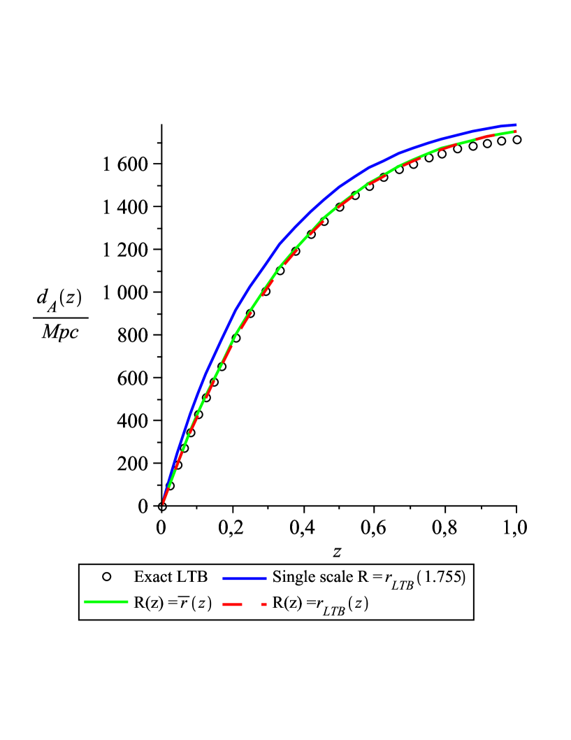
Figure 1: The angular diameter distance $d_{A}(z)$ of the bubble model with $H_{0}(r)=H+\Delta He^{-r/r_{0}}$, where $H+\Delta H=65.5{\rm~{}km/s/Mpc}$, $\Delta H=16.8{\rm~{}km/s/Mpc}$ and $r_{0}=1400{\rm~{}Mpc}$. The black circles represent the exact LTB solution, whereas the blue, green and red curves correspond to the following coarse grained cases: Blue $-$ a single averaging scale, chosen to be $r_{{\rm LTB}}(1.755)=4944{\rm~{}Mpc}$, where $z=1.755$ is the redshift of the farthest supernova in the sample. Green $-$ the averaged physical distance $\bar{r}(z)$ as the running smoothing scale. Red $-$ the exact physical distance $r_{{\rm LTB}}(z)$ as the running smoothing scale.

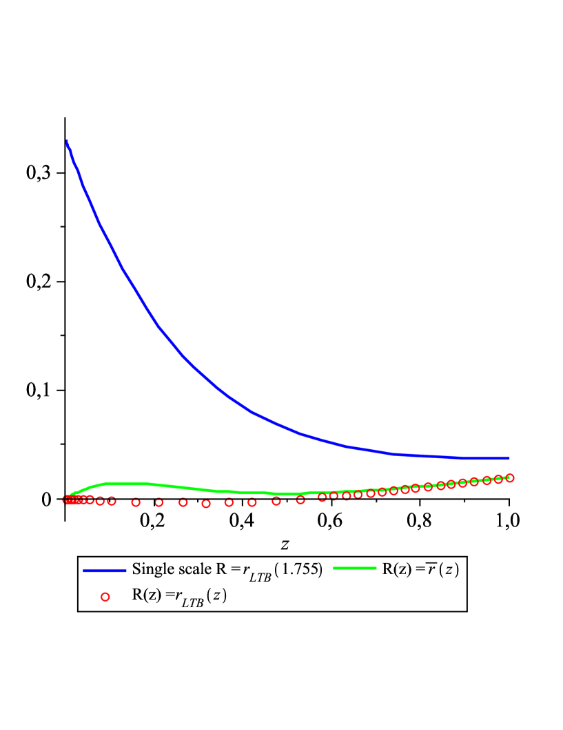
Figure 2: The relative deviation $(\bar{d}_{A}(z)-d_{A}(z))/d_{A}(z)=(\bar{d}_{L}(z)-d_{L}(z))/d_{L}(z)$ of the averaged angular diameter (or luminosity) distance $\bar{d}_{A}(z)$ from the exact value $d_{A}(z)$ for the bubble model of Sect. 3.3 in the following cases: Blue $-$ a single averaging scale, chosen to be $r_{{\rm~{}LTB}}(1.755)=4944{\rm~{}Mpc}$, where $z=1.755$ is the redshift of the farthest supernova in the sample. Green $-$ the averaged physical distance $\bar{r}(z)$ as the running smoothing scale. Red $-$ the exact physical distance $r_{{\rm LTB}}(z)$ as the running smoothing scale.

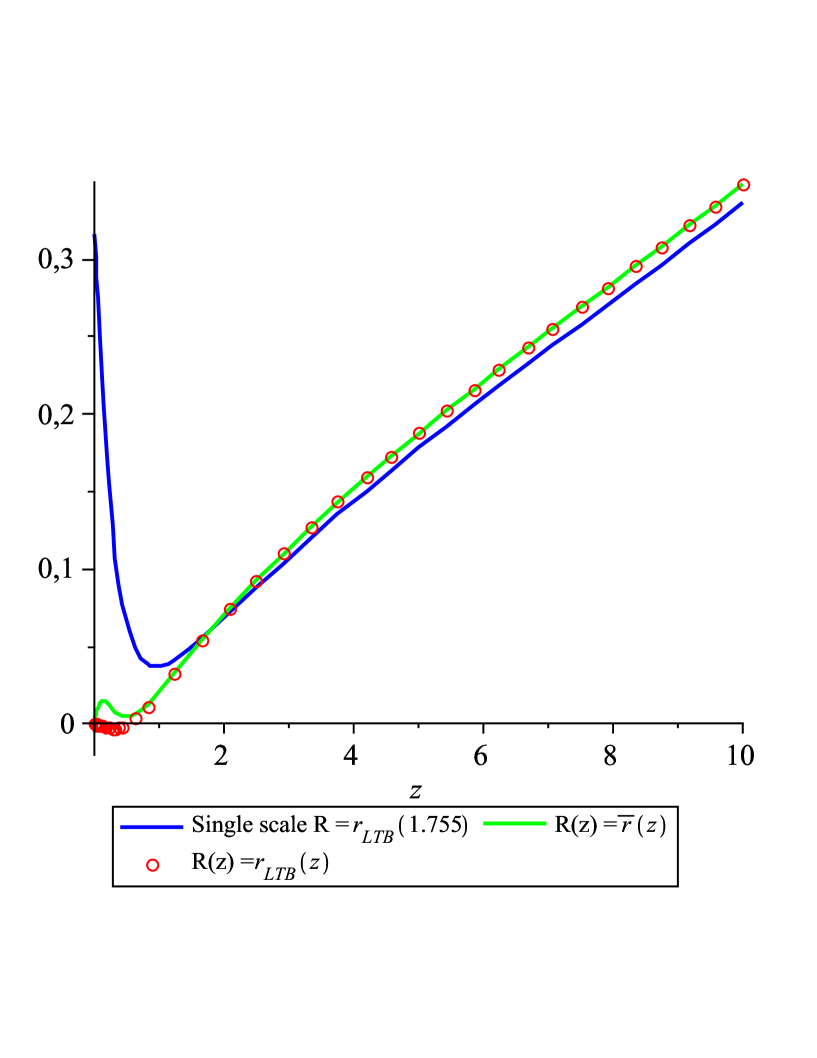
Figure 3: Same as in Figure 2, but for larger redshift range, $z=0...10$.

3.4 Periodic inhomogeneities as a toy model for structure

Perhaps the closest representative of structure under the assumption of spherical symmetry is achieved with a periodic boundary condition function $H_{0}(r)$ [33]. Hence, we take

$$H_{0}(r)=H+\Delta H\sin{r/r_{0}}~{},$$ (54)

where the values $H=65.5~{}{\rm{km/s/Mpc}}$, $\Delta H=1.64~{}{\rm{km/s/Mpc}}$ and $r_{0}=95~{}{\rm{Mpc}}$ have been chosen to make the plots as illustrative as possible. We do not consider more intense inhomogeneities in order to keep the relation $r_{{\rm{LTB}}}(z)$ single-valued to the redshift $z=1$.

We plot the exact angular diameter distance of this model with the averaged results in Fig. 4, and the relative deviation $(\bar{d}_{A}(z)-d_{A}(z))/d_{A}(z)$ in Fig. 5, for each of the different cases introduced in Sect. 3.1.

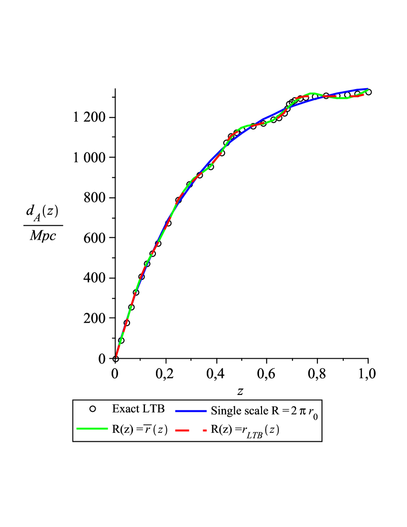
Figure 4: The angular diameter distance $d_{A}(z)$ for the model of Sect. 3.4 with periodic inhomogeneities, $H_{0}(r)=H+\Delta H\sin(r/r_{0})$, where $H=65.5{\rm~{}km/s/Mpc}$, $\Delta H=1.64{\rm~{}km/s/Mpc}$ and $r_{0}=95{\rm~{}Mpc}$. The black circles represent the exact LTB solution, whereas the blue, green and red curves correspond to the following coarse grained cases: Blue $-$ a single averaging scale, chosen to be one oscillation period $2\pi r_{0}=598{\rm~{}Mpc}$. Green $-$ the averaged physical distance $\bar{r}(z)$ as the running smoothing scale. Red $-$ the exact physical distance $r_{{\rm LTB}}(z)$ as the running smoothing scale.

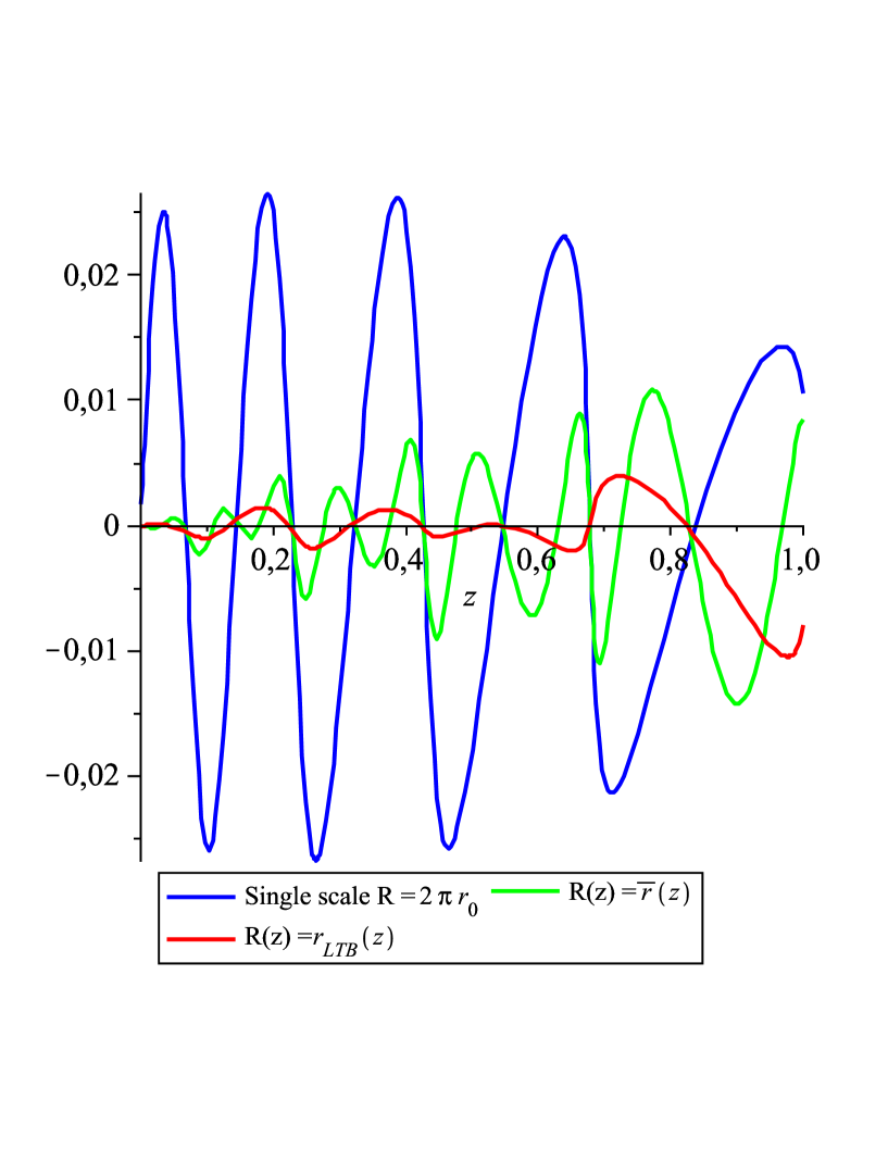
Figure 5: The relative deviation $(\bar{d}_{A}(z)-d_{A}(z))/d_{A}(z)=(\bar{d}_{L}(z)-d_{L}(z))/d_{L}(z)$ of the averaged angular diameter (or luminosity) distance $\bar{d}_{A}(z)$ from the exact value $d_{A}(z)$ for the model of Sect. 3.4 in the following cases: Blue $-$ a single averaging scale, chosen to be one oscillation period $2\pi r_{0}=598{\rm~{}Mpc}$. Green $-$ the averaged physical distance $\bar{r}(z)$ as the running smoothing scale. Red $-$ the exact physical distance $r_{{\rm LTB}}(z)$ as the running smoothing scale.

3.5 Discussion of the results

Let us discuss here the results of Sects. 3.2, 3.3 and 3.4 by taking each coarse graining level of Sect. 3.1 into separate consideration:

3.5.1 $R(z)=R$ $-$ Single scale

In this case, already the general form of the luminosity distance (40) reveals the essential point: averaging over a single scale is equivalent to using the perfectly homogeneous and flat matter dominated FRW model. The freedom to choose the averaging scale $R$ only corresponds to fixing the value of the effective Hubble constant $H_{0}(R)$ in Eq. (40).

The supernova data fit in the bubble model of Sect. 3.3 shows that when averaging over the domain that contains all the supernovae in the sample ($R=4944~{}{\rm Mpc}$), the resulting $\chi^{2}=4.35$ represents a huge deviation from the exact result, $\chi^{2}=1.12$. We get a better fit by choosing $R=905~{}{\rm{Mpc}}$, because this gives the effective Hubble constant in Eq. (40) its best fit value for the flat matter dominated FRW case, $H_{0}(905~{}{\rm{Mpc}})=57.5~{}{\rm{km/s/Mpc}}$. However, even this value gives $\chi^{2}=2.06$, which is still a way too large deviation from the actual result. Besides, we have no a priori physical justification to pick up the particular averaging scale $R=905~{}{\rm{Mpc}}$. Overall, it is clear that no single averaging scale can give an acceptable approximation for the bubble model.

Perhaps the most interesting feature of the single scale case becomes evident in Figs. 4 and 5: even though the model of Sect. 3.4 with periodic inhomogeneities is homogeneous on large scales, the single averaging scale still leads to unwanted deviations. Whether it is an artifact of the employed spherical symmetry, with light inevitably propagating through all the layers of structure, or a more general phenomenon, remains an open question.

Altogether, the expression of the averaged luminosity distance (40), along with its Taylor expansion (44), and the figures 1 - 5 all confirm the conclusion that averaging over a single scale gives a too coarse-grained description at least for the flat LTB universe. The inadequacy of the averaging procedure to account for the observations in the LTB universe was already suggested in Ref. [27], but our results bring out the essential point that the conclusion is valid only under the assumption of a single smoothing scale, as we next discuss.

3.5.2 $R(z)=\bar{r}(z)$ $-$ Running scale with averaged geodesics

It has been speculated that averaging cosmological inhomogeneities would be useful only when applied to systems with statistically homogeneous distribution of small scale irregularities [19]. Nevertheless, our results indicate that it is possible to exploit averaging also for large scale inhomogeneities, if the single smoothing scale $R$ is promoted to a redshift dependent function $R(z)$.

On physical grounds, one could have expected some improvement in accuracy of the observables when the single averaging scale $R$ is replaced by the averaged present-day physical distance (37) to each object at redshift $z$. However, the amount of precision achieved with this generalization is both surprising and a very welcome result. Indeed, the congruence between this approximation and the exact results is evident in all of the comparisons made in Sects. 3.2, 3.3 and 3.4 as we next specify in more detail.

When comparing the Taylor expanded luminosity distance (• ‣ 3.2) with the expansion of the exact LTB case (• ‣ 3.2), one sees that to second order the results are almost identical. They become exactly identical if we take $R=0$ as the averaging scale for the geodesics, corresponding to the use of the local Hubble parameter $H_{0}(0)$ in Eq. (37), or if $H_{0}(R)=H_{0}(0)$, as is the case for periodic inhomogeneities of Sect. 3.4. Moreover, even the third order terms carry the same functional dependence on $H_{0}(r)$ as the exact case of Eq. (• ‣ 3.2), albeit with slightly different prefactors.

The supernova data fit in the bubble model of Sect. 3.3 illustrates the power of the running scale approach in practical applications. When employing the running scale, the goodness of the fit changes from the puny $\chi^{2}=4.35$ of the single scale case to the excellent fit $\chi^{2}=1.11$, which is within one percent of the correct result $\chi^{2}=1.12$; the improvement is manifest in Figs. 1 and 2 as well. The result also elucidates how the scale dependence can produce apparent acceleration even in the absence of backreaction; for a thorough discussion of the apparent acceleration, see page 9 of Ref. [27]. Anyhow, in the real universe, one could expect the effective acceleration to arise from the interplay between scale dependence and backreaction, but the possibility remains that either $-$ or neither for that matter $-$ of them plays the dominant role.

The toy model of structure in Sect. 3.4 also manifests the advantage of the running smoothing scale: it is evident in Figs. 4 and 5 that the running scale follows the oscillations of the exact observables whereas the single scale case simply fails to.

Problems arise, when going beyond the supernova fits to higher redshifts. Indeed, Fig. 3 reveals that at $z\gtrsim 2$ the running scale falls short of the $\mathcal{O}(1\%)$ accuracy compared to the exact observables. There is a plausible physical explanation for this: in the employed LTB model, the growth of inhomogeneities backwards in time makes them more important at higher redshifts and cannot be encapsulated in the present-day spatial averages. One can still argue that in a more realistic model the problem would be alleviated, since the inhomogeneities of the real universe are expected to grow forwards in time. Overall, we suppose the averaging with the running scale would be conceivable at least up to $z\sim 2$; for higher redshifts, one could then use coarser approximations, such as the perturbed FRW models, presuming inhomogeneities really were of less importance in the past.

It would, nevertheless, be desirable to remedy the problems at higher redshifts. For this, we have considered various forms for the running smoothing scale $R(z)$, beyond the ones introduced in Sect. 3.1. The outcome is that there seems to be no functions $R(z)$ that would both have a physical basis, and improve the approximation over the whole range of redshifts. In particular, it seems difficult to allow for the time evolution of the universe within the running averaging scale approach. Perhaps a better way to take into account the time evolution would be to average over the past light cone. However, this would require a complete revision of the basic formalism.

Finally, a great virtue of using the geodesics of the averaged metric is that one does not need to solve the exact geodesic equations. Moreover, one can improve the accuracy of this method by iterative use of the averaged distance-redshift relation (37), as argued in the paragraph before Eq. (41).

3.5.3 $R(z)=r_{{\rm{LTB}}}(z)$ $-$ Running scale with exact geodesics

There are two conceptual steps in coarse graining needed to calculate the observables [32]. Firstly, the step from the exact Einstein equations to the Buchert equations, and secondly, the step from the exact metric (1) to the average metric (34). To quantify the approximation of the latter step, we studied a case where only the field equations have been averaged, but instead of the average metric, the exact metric determines the geodesics.

The outcome is that there are only minor deviations in the observables between the use of the averaged and the exact geodesics. This becomes apparent in the congruence between the Taylor expansions of the luminosity distance (• ‣ 3.2) and (• ‣ 3.2), between the resulting $\chi^{2}$ for the supernova data fit in Eqs. (52) and (53), and between the red and green curves in Figs. 1 - 5. Although corresponding only to a slight correction, it is still evident in all of these comparisons that the exact physical distance gives the most accurate approximation. Anyway, due to the good congruence of the results between the averaged and the exact geodesics, the feasibility becomes the deciding factor. Indeed, in more realistic models of the universe, the exact geodesics are beyond computation. Overall, perhaps the best solution in practice is to use the averaged geodesics and, if needed, use Eq. (37) iteratively as explained in Sect. 3.1.

4 Conclusions

We have considered the role of scale dependence in the Buchert averaging formalism, using the spherically symmetric and spatially flat LTB dust universe as a testing ground. The vanishing of both the backreaction and the spatial curvature scalar ${}^{(3)}R$ makes this an ideal model to capture the effect of the averaging scale on the observables, because then the only difference from the flat FRW model is the explicit dependence on the smoothing scale. From the resulting Buchert equations (31), (32), (33) and the average metric (34), we have derived the luminosity and angular diameter distances (38) and (39), carrying the scale dependence as well. By employing a redshift dependent averaging scale $R(z)$, we have compared these observables to the exact expressions (11) and (12). The physical reason to use a different averaging scale for each object at redshift $z$ is clear: the distance the observed light propagates depends on how far the object is.

Our principal result is that when the conventional single averaging scale is replaced by the physical distance to each object at redshift $z$, the relations (38) and (39) become significantly closer to the actual observables without complicated computations. Although some improvement could be expected on physical grounds, the ${\mathcal{O}}(1\%)$ precision at $z<2$ makes the result a welcome surprise. Indeed, contrary to some previous speculations [19, 27], the result suggests that the averaging procedure can be exploited for large scale inhomogeneities, presuming the running smoothing scale is employed. Although considered merely under the assumption of spherical symmetry, we expect the running scale to show its full advantage only when applied to more irregular large scale inhomogeneities, such as the recently observed voids [21, 22]. Naturally, the running scale can also be applied even if a single scale would suffice, since then it reduces to give the same predictions as the single scale approach.

By Taylor expanding the averaged observables and their exact counterparts, we have demonstrated the increase in accuracy for generic inhomogeneities up to redshifts $z\sim 0.2$. In addition, we have numerically confirmed it for redshifts up to $z\sim 2$ using two explicit inhomogeneity profiles: a bubble inhomogeneity that fits the supernova observations and periodic inhomogeneities as a toy model for structure. Within the bubble model, we found that the running smoothing scale can account for the apparent acceleration even without backreaction. Consequently, it could be at least as important as the backreaction in explaining dark energy as an inhomogeneity induced illusion.

At redshifts $z\gtrsim 2$, the method breaks down. The plausible physical explanation for this is that the present-day spatial averages cannot capture the time evolution of the exact model. Whether the problem can be solved within the already developed formalism, or a generalized approach such as averaging over the light cone would be needed, is something we hope to address in a future work. In any case, the time evolution of the flat LTB model is contrary to the observed structure formation, since the inhomogeneities of the model grow towards large redshifts. Hence, perhaps in the real universe one could apply the running scale in averaging at low redshifts, and at higher redshifts, resort to the conventional perturbed FRW models.

We have employed two ways to compute the present-day physical distance $R(z)$ to objects with redshift $z$: firstly, using the geodesics of the average metric and, for comparison, using the geodesics of the exact metric. The outcome is that using the exact geodesics gives only a marginal correction compared to the averaged geodesics and, requiring the exact solution, would in general lead to complicated computations. Overall, maybe the best method in practice would be an iterative use of the averaged distance-redshift relation (37), as explained in Sect. 3.1.

Finally, there are problems in cosmological averaging we have not addressed in this work (see [19, 23, 25, 34, 35, 36, 37, 38]). Perhaps the most notable one within the Buchert formalism is that the averaged equations (13), (14) and (15) contain three equations for four unknowns. Therefore, more information is in general needed to solve the equations. Whether this makes the whole approach impractical in calculating observables outside the exact solutions of the Einstein equations, is an open question.

- [1] A. G. Riess et al. [Supernova Search Team Collaboration], “Type Ia Supernova Discoveries at From the Hubble Space Telescope: Evidence for Past Deceleration and Constraints on Dark Energy Evolution”, Astrophys. J. 607 (2004) 665 [arXiv:astro-ph/0402512].
- [2] D. J. Eisenstein et al., “Detection of the Baryon Acoustic Peak in the Large-Scale Correlation Function of SDSS Luminous Red Galaxies”, Astrophys. J. 633 (2005) 560 [arXiv:astro-ph/0501171].
- [3] D. N. Spergel et al., “Wilkinson Microwave Anisotropy Probe (WMAP) three year results: Implications for cosmology”, arXiv:astro-ph/0603449.
- [4] E. J. Copeland, M. Sami and S. Tsujikawa, “Dynamics of dark energy”, Int. J. Mod. Phys. D 15 (2006) 1753 [arXiv:hep-th/0603057].
- [5] N. Straumann, “Dark energy: Recent developments”, Mod. Phys. Lett. A 21 (2006) 1083 [arXiv:hep-ph/0604231].
- [6] V. Sahni and A. Starobinsky, “Reconstructing dark energy”, Int. J. Mod. Phys. D 15 (2006) 2105 [arXiv:astro-ph/0610026].
- [7] A. Blanchard, M. Douspis, M. Rowan-Robinson and S. Sarkar, “An alternative to the cosmological ’concordance model’ ”, Astron. Astrophys. 412 (2003) 35 [arXiv:astro-ph/0304237].
- [8] P. Hunt and S. Sarkar, “Multiple inflation and the WMAP ’glitches’ ”, Phys. Rev. D 70 (2004) 103518 [arXiv:astro-ph/0408138].
- [9] P. Hunt and S. Sarkar, “Multiple inflation and the WMAP ’glitches’ II. Data analysis and cosmological parameter extraction”, arXiv:0706.2443 [astro-ph].
- [10] J. F. Pascual-Sanchez, “Cosmic acceleration: Inhomogeneity versus vacuum energy”, Mod. Phys. Lett. A 14 (1999) 1539 [arXiv:gr-qc/9905063].
- [11] M. N. Celerier, “Do we really see a cosmological constant in the supernovae data ?”, Astron. Astrophys. 353 (2000) 63 [arXiv:astro-ph/9907206].
- [12] K. Tomita, “A Local Void and the Accelerating Universe”, Mon. Not. Roy. Astron. Soc. 326 (2001) 287 [arXiv:astro-ph/0011484].
- [13] H. Iguchi, T. Nakamura and K. i. Nakao, “Is dark energy the only solution to the apparent acceleration of the present universe?”, Prog. Theor. Phys. 108 (2002) 809 [arXiv:astro-ph/0112419].
- [14] A. Krasinski, “Inhomogeneous Cosmological Models”, Cambridge University Press (1997).
- [15] J. Plebanski and A. Krasinski, “An Introduction to General Relativity and Cosmology”, Cambridge University Press (2006).
- [16] G. Lemaitre, Annales Soc. Sci. Brux. Ser. I Sci. Math. Astron. Phys. A 53 (1933) 51. For an English translation, see: G. Lemaitre, “The Expanding Universe”, Gen. Rel. Grav. 29 (1997) 641.
- [17] R. C. Tolman, “Effect Of Inhomogeneity On Cosmological Models”, Proc. Nat. Acad. Sci. 20 (1934) 169.
- [18] H. Bondi, “Spherically Symmetrical Models In General Relativity”, Mon. Not. Roy. Astron. Soc. 107 (1947) 410.
- [19] S. Räsänen, “Accelerated expansion from structure formation”, JCAP 0611 (2006) 003 [arXiv:astro-ph/0607626].
- [20] D. J. Schwarz, “Accelerated expansion without dark energy”, arXiv:astro-ph/0209584.
- [21] L. Rudnick, S. Brown and L. R. Williams, “Extragalactic Radio Sources and the WMAP Cold Spot”, arXiv:0704.0908 [astro-ph].
- [22] A. V. Tikhonov, “Voids in the SDSS Galaxy Survey”, Astron. Lett. 33 (2007) 499 [arXiv:0707.4283 [astro-ph]].
- [23] G. F. R. Ellis and T. Buchert, “The universe seen at different scales”, Phys. Lett. A 347 (2005) 38 [arXiv:gr-qc/0506106].
- [24] T. Buchert, “On average properties of inhomogeneous fluids in general relativity. I: Dust cosmologies”, Gen. Rel. Grav. 32 (2000) 105 [arXiv:gr-qc/9906015].
- [25] T. Buchert, “Dark Energy from Structure - A Status Report”, arXiv:0707.2153 [gr-qc].
- [26] A. Paranjape and T. P. Singh, “The Possibility of Cosmic Acceleration via Spatial Averaging in Lemaitre-Tolman-Bondi Models”, Class. Quant. Grav. 23 (2006) 6955 [arXiv:astro-ph/0605195].
- [27] K. Enqvist and T. Mattsson, “The effect of inhomogeneous expansion on the supernova observations”, JCAP 0702 (2007) 019 [arXiv:astro-ph/0609120].
- [28] J. Silk, “Large-scale inhomogeneity of the Universe - Spherically symmetric models”, Astron. Astrophys. 59 (1977) 53
- [29] G. F. R. Ellis, in Proc. School Enrico Fermi, “ General Relativity and Cosmology ”, Ed. R. K. Sachs, Academic Press (New York 1971)
- [30] P. S. Apostolopoulos, N. Brouzakis, N. Tetradis and E. Tzavara, “Cosmological acceleration and gravitational collapse”, JCAP 0606 (2006) 009 [arXiv:astro-ph/0603234].
- [31] T. Kai, H. Kozaki, K. i. nakao, Y. Nambu and C. M. Yoo, “Can inhomogeneties accelerate the cosmic volume expansion?”, Prog. Theor. Phys. 117 (2007) 229 [arXiv:gr-qc/0605120].
- [32] A. Paranjape and T. P. Singh, “Explicit Cosmological Coarse Graining via Spatial Averaging”, arXiv:astro-ph/0609481.
- [33] T. Biswas, R. Mansouri and A. Notari, “Nonlinear Structure Formation and Apparent Acceleration: an Investigation”, arXiv:astro-ph/0606703.
- [34] A. Paranjape and T. P. Singh, “The Spatial Averaging Limit of Covariant Macroscopic Gravity - Scalar Corrections to the Cosmological Equations”, Phys. Rev. D 76 (2007) 044006 [arXiv:gr-qc/0703106].
- [35] M. N. Celerier, “The Accelerated Expansion of the Universe Challenged by an Effect of the Inhomogeneities. A Review”, arXiv:astro-ph/0702416.
- [36] A. A. Coley, “Averaging and cosmological observations”, arXiv:0704.1734 [gr-qc].
- [37] N. Brouzakis, N. Tetradis and E. Tzavara, “The Effect of Large-Scale Inhomogeneities on the Luminosity Distance”, JCAP 0702 (2007) 013 [arXiv:astro-ph/0612179].
- [38] N. Brouzakis, N. Tetradis and E. Tzavara, “Light Propagation and Large-Scale Inhomogeneities”, arXiv:astro-ph/0703586.