Theoretical analysis of the optimal conditions
for photon-spin quantum state transfer
Abstract
We analyzed the yield and fidelity of the quantum state transfer (QST) from a photon polarization qubit to an electron spin qubit in a spin-coherent photo detector consisting of a semiconductor quantum dot. We used a model consisting of the quantum dot, where the QST is carried out, coupled with a photonic cavity. We determined the optimal conditions that allow the realization of both high-yield and high-fidelity QST.
pacs:
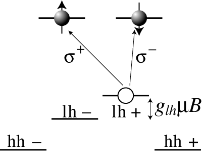
03.67.-a, 68.65.Hb, 72.25.FeA quantum repeater is a promising technology Briegel et al. (1998); Childress et al. (2005); Taylor et al. (2005) which makes it possible to drastically expand the distance of quantum key distribution as well as to realize scalable quantum networks. The quantum repeater requires not only messenger qubits but also processing qubits. A photon is, of course, the most convenient candidate for the messenger qubit Gisin et al. (2002); Gobby et al. (2004); however, it is not suitable to be used as a processing qubit because quantum information storage and two-qubit quantum operations are very difficult to perform. On the other hand, an electron spin in a semiconductor quantum dot is one of the most convenient candidates for processing qubits since one- and two-bit quantum gate operations can now be performed through the application of electric and/or magnetic fields Loss and DiVincenzo (1998); Taylor et al. (2003); Petta et al. (2005a, b). Therefore, it is important to investigate the possibility of a photon-spin quantum state transfer (QST) Vrijen and Yablonovitch (2001); Duan et al. (2001); Kosaka et al. (2003); Muto et al. (2005) which would transfer quantum information from a photon-polarization (photon qubit) to an electron-spin (spin qubit), as an interface device for quantum repeaters. Such a photon-spin QST can be performed using a semiconductor spin-coherent photo detector, as proposed by Vrijen and Yablonovitch Vrijen and Yablonovitch (2001), who showed that the well-known optical orientation in a semiconductor heterostructure can be used for QST with the help of -factor engineering Kiselev et al. (1998); Ivchenko and Kiselev (1998); Matveev et al. (2000); Kosaka et al. (2001); Salis et al. (2001, 2003); Nitta et al. (2003); Lin et al. (2004); Nitta et al. (2004) and strain engineering Lin et al. (1991); Nakaoka et al. (2004, 2005). The photo detector has a quantum dot whose energy levels are shown in Fig. 1(a). The -factor of the electron spin is tuned to zero (). By using strain engineering and applying a magnetic field, we can arrange the light-hole state to the topmost level of the valence band. According to the selection rule Vrijen and Yablonovitch (2001), a spin-up (down) electron () is excited by a right-handed (left-handed) circularly polarized photon () from the state. As shown in Fig. 1(b), the quantum dot is connected to the continuum of the hole state and the created hole extracted from the dot to the continuum. By eliminating the hole in the state, we complete the QST from the photon qubit to the spin qubit .
One of the obstacles to high-fidelity QST in a spin-coherent semiconductor photo detector is the exchange interaction between the electron and the simultaneously created hole. The electron-hole exchange interaction disturbs the electron spin state and decreases fidelity. In our previous work Rikitake and Imamura (2006), we proposed the use of resonant tunneling in a double-well structure Gurvitz et al. (1991); Cohen et al. (1993) in order to avoid the electron-hole exchange interaction. However, we considered the QST process only after the creation of the exciton, and did not take into account the exciton creation process itself; thus, our previous work lacked discussion about the efficiency, or yield of the QST. In the present study, we analyzed the QST process from the photon qubit to the spin qubit in a spin-coherent semiconductor photo detector, considering the whole QST process from the input photon to the generated electron spin via the dot exciton state. We present here the conditions necessary to produce a high-yield, high-fidelity QST.
| (a) | (b) |
|---|---|
 |
 |
We examined the model shown in Fig. 2. The quantum dot is located in the photonic cavity. The quantum dot is also connected to the continuum of the hole through the tunneling barrier in order to extract the created hole. The input photon propagates the -axis and enters the cavity (one-sided cavity)Kojima et al. (2003); Kojima and Tomita (2007); Koshino and Ishihara (2004). The cavity photon excites the electron-hole pair or exciton in the dot. By applying appropriate selection rule, the electron spin state is determined by the input photon polarization state. Once the electron-hole pair is excited in the quantum dot, the created hole is extracted to the continuum and the electron spin is left in the dot. The QST process is then completed. In addition to the above processes, we also considered the electron-hole exchange interaction and the spontaneous emission from the dot. The electron-hole exchange interaction modifies the orientation of the electron-spin, while the hole is in the dot and therefore reduces the fidelity of the QST. Spontaneous emission leads to a decrease in yield.
The state vector of the system under consideration is expressed as
| (1) |
where denotes the input/output photon state at position and polarization ; the cavity photon with polarization ; the exciton state in the dot with electron spin state ; the external noncavity photon ( represents the wave number and corresponding polarization); and the state in which the electron with spin state is in the dot and the hole is in the continuum state . Here , , , , and are coefficients to be determined by solving the Schrödinger equation. For later use, we name the state represented by the last term in Eq. (1) the “spin state”.

The Hamiltonian of the system is given by
| (2) |
each of whose terms are defined as follows, under the condition :
| (3) | ||||
| (4) | ||||
| (5) | ||||
| (6) | ||||
| (7) | ||||
| (8) | ||||
| (9) | ||||
| (10) | ||||
| (11) |
The Hamiltonian for the input/output photon is , where is wave number of the input/output photon, and is the speed of light. Note that we use the wave number representation instead of the position representation used in Eq. (1). The interaction between the input/output photon and the cavity photon is represented by . With respect to the coupling constants in , we use the flat-band assumption Koshino and Ishihara (2004), where is the cavity damping rate. The Hamiltonian for the cavity photon is , and denotes the energy of the cavity mode photon. The cavity photon excites the dot exciton; this excitation is represented by , which is characterized by the cavity-dot coupling . The index of the photon polarization represents the selection rule: . The Hamiltonian for the dot exciton is , is the excitation energy, is the electron-hole exchange interaction which flips the electron spin state, and represents the opposite spin to . The spontaneous emission process from the dot exciton is represented as . The emitted photon escapes to the external noncavity photon mode with energy and is the Hamiltonian of the noncavity photon. The extraction of the created hole in the dot is represented by the hole’s tunneling Hamiltonian , where is the tunneling matrix elements. The Hamiltonian for the spin state where the electron spin is left in the dot and the hole is extracted to the continuum is . The energy of the electron in the dot is , and that of the hole in the continuum state is .
In order to analyze the QST process in this model, we must consider the scattering problem from the initial input photon state to the final spin state. The initial state at is written as
| (12) |
where and are the probability amplitudes which characterize the superposition state of the photon qubit . The coefficient represents the input photon wave packet. We consider a Gaussian wave packet defined as
| (13) |
where () is the center position of the wave packet at , the center frequency of the photon and the bandwidth of the input photon.
The extraction process of the hole is characterized by the spectral function defined by . In the present analysis, we treat this spectral function as the constant . This treatment corresponds to the Markov approximation with respect to the extraction process, and the constant represents the extraction rate of the hole from the dot to the continuum. We also apply the Markov approximation to the spontaneous emission process; that is, we treat the spectral function as the constant , where is the spontaneous emission rate of the dot exciton.
By employing the Schrödinger equation and the above Markov approximations, we obtain the equations for the probability amplitudes of the cavity photon and the dot exciton as,
| (14) | ||||
| (15) |
By setting the input photon polarization and the shape of the wave packet as Eq. (13), we can solve these equations and obtain the time evolutions of and . The probability amplitude of the spin state is obtained from that of the exciton state as
| (16) |
Let us consider the final state of the system for . The final electron spin state is characterized by the reduced density matrix defined as
| (17) |
for . The efficiency of the QST is represented by the yield defined as , which represents the probability that the electron spin is left in the dot at the final state. Using , we can define the fidelity of the QST as , where is the ideal spin state. Here we note that the fidelity is normalized by yield ; that is, we take into account the fidelity only of the generated spin at the final state. Straightforward calculations then give us the expressions for the yield and fidelity as
| (18) | ||||
| (19) |
respectively, where . The coefficients () are defined as follows:
| (20) |
where
| (21) |
The parameters we used in the present paper are as follows: input photon bandwidth , electron-hole exchange interaction , and spontaneous emission rate . We used the typical values in a GaAs quantum dot for and Gammon et al. (1996); Takagahara (2000); Bayer et al. (2002). For the cavity damping rate , we considered two cases: the weak cavity damping case , and the strong cavity damping case . We also assumed the resonance condition , and the input photon polarization was .
| (a) | (b) |
|---|---|
 |
 |
In what follows, we will show the results for yield and fidelity in the weak () and strong () cavity damping cases. We will also discuss the effects of spontaneous emission.
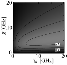
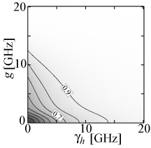
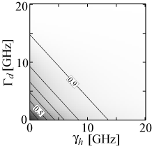
Let us discuss the yield and fidelity of the QST in the weak cavity damping case . In Fig. 3 (a), we show the contour plot of the yield as a function of the extraction rate of hole and cavity-dot coupling . We take . As shown in the figure, the yield is much less than the unity because the cavity damping rate is so small that most input photons can not enter the cavity. Figure 3(b) is the contour plot of the fidelity as a function of and . Note that the fidelity is suppressed in the vicinity of the origin, where the dwell time of the hole is much longer than the precession period of the electron spin due to the electron-hole exchange interaction.
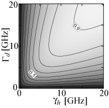
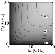
In the strong cavity damping case , it is useful to introduce the effective dipole relaxation rate defined as , which represents the enhanced spontaneous emission rate of the exciton due to the coupling with the cavity photon. Figure 4(a) shows the contour plot of the yield as a function of and with . To consider in detail the effects of on the yield, let us fix at a certain value and increase from zero. As increases, the recombination of the dot exciton is suppressed, hence the yield increases with increasing . However, the increase of prevents the creation of the dot exciton, which suppresses the yield for large values of . Therefore, the yield takes its maximum value at . The condition is also important for producing a high yield in order to transfer energy effectively from the input photon to the exciton. The condition for this high yield is summarized as .
Fig. 4(b) is the contour plot of the fidelity. Note that the fidelity is reduced from unity for . The lifetime of the exciton state is given as for the impulse-like input photon wave packet in the case of strong cavity damping. In order to avoid the effects of the electron-hole exchange interaction, the lifetime of the exciton state should be much shorter than the characteristic time of the exchange interaction . Therefore, the condition is required for a high-fidelity QST.
| (a) | (b) |
|---|---|
 |
 |
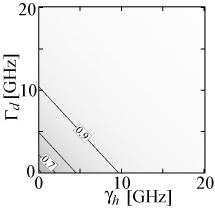
Let us now examine the effects of spontaneous emission on the yield and fidelity. Since we have taken the spontaneous emission rate to be much smaller than the input photon bandwidth in the above discussions, the yield and fidelity are not significantly affected by spontaneous emission. Figures 5(a) and (b) show the contour plots of yield and fidelity, respectively, in the case of a relatively large spontaneous emission rate . When the spontaneous emission process is dominant, the emission occurs before the hole is extracted from the dot, and the yield decreases as the spontaneous emission rate increases, as shown in Fig. 5(a). However, even in the case of a large spontaneous emission rate, we can obtain high yield by setting and to be much greater than , and by satisfying the matching condition, . If we compare Figs. 4(b) and 5(b), we recognize that the fidelity is slightly improved by taking a large . The lifetime of the exciton is shortened by the spontaneous emission, and the spin-flip process of the electron-hole exchange interaction is therefore suppressed and fidelity is improved.
With respect to the relationship between the results obtained in the present study and those of our previous work Rikitake and Imamura (2006), we must point out that, in our previous paper, we analyzed the fidelity of the QST by considering the QST process after the creation of the dot exciton, but did not consider the yield of the QST. We concluded in that work that the hole should be extracted from the dot as rapidly as possible in order to achieve high fidelity, which is consistent with the present results. That is, we can achieve higher fidelity as the extraction rate of the hole increases, as shown in Fig. 4 (b). However, too large a value of leads to a decrease in the yield, as shown in Fig. 4 (a). In order to obtain both high yield and high fidelity, and should be as large as possible while satisfying the matching condition .
| (a) | (b) |
|---|---|
 |
 |
Finally, we estimated the yield and fidelity of the QST in a single quantum dot-semiconductor microcavity coupling system Reithmaier et al. (2004); Yoshie et al. (2004); Peter et al. (2006). Let us consider the GaAs quantum dot formed by monolayer fluctuations in the Al0.8In0.2As/GaAs/Al0.8In0.2As quantum well (QW). By adjusting the thickness of the QW appropriately, We can set the electron spin -factor in the QW to zero Nakayama et al. (1992) and the energy levels shown in Fig. 1(a) can be realized. The excitation energy of the dot exciton is estimated about . Note that as shown in Fig. 1(b), the continuum of the hole state should be attached via AlInAs barrier layer to extract the created hole. As the cavity we consider the micropllar cavity having top and bottom AlxGa1-xAs/AlAs () Bragg mirrorsAndreani et al. (1999), and the QW is located in the cavity. The cavity-dot coupling is given by , where is the exciton oscillator strength, the effective modal volume, the free electron mass, the electron charge, the electric constant, and the relative permittivity. The oscillator strength of transition from heavy heavy hole states (denoted as hh in Fig. 1(a)) in a GaAs quantum dot more than is theoretically predicted Andreani et al. (1999) and experimentally observedPeter et al. (2006). Because we use the transition from the lh+ state and its oscillator strength is roughly given by , therefore we can assume here. With the cavity modal value , the cavity-dot coupling becomes . For the cavity decay rate, we assume , and this value corresponds to the cavity Q-factor which now be realized in micropillar cavitiesReitzenstein et al. (2006). The extraction rate of the hole is a tunable parameter by changing the barrier width. Here we take so that the matching condition is satisfied. With the other parameters, input photon bandwidth , electron-hole exchange interaction , and and spontaneous emission rate , we then obtain yield and fidelity .
In conclusion, we have analyzed the yield and fidelity of the QST from the photon qubit to the spin qubit in a spin-coherent semiconductor photo detector. By considering a model in which the quantum dot is coupled with the photonic cavity, we determined the optimal conditions for high-yield and high-fidelity QST. Briefly, the cavity damping rate should be larger than the input photon bandwidth, , and the matching condition, , between the extraction rate of the hole and the effective dipole relaxation rate should be also satisfied in order to obtain high yield. For high-fidelity QST, a small electron-hole exchange interaction is preferred compared to the extraction rate of the hole and the effective dipole relaxation rate, .
The authors would like to thank T. Takagahara for valuable discussions. This work was supported by CREST, MEXT. KAKENHI (No. 16710061), the NAREGI Nanoscience Project, and a NEDO Grant.
References
- Briegel et al. (1998) H. Briegel, W. Dur, J. Cirac, and P. Zoller, Phys. Rev. Lett. 81, 5932 (1998).
- Childress et al. (2005) L. Childress, J. Taylor, A. Sorensen, and M. Lukin, Phys. Rev. A 72, 052330 (2005).
- Taylor et al. (2005) J. Taylor, W. Dur, P. Zoller, A. Yacoby, C. Marcus, and M. Lukin, Phys. Rev. Lett. 94, 236803 (2005).
- Gisin et al. (2002) N. Gisin, G. Ribordy, W. Tittel, and H. Zbinden, Rev. Mod. Phys. 74, 145 (2002).
- Gobby et al. (2004) C. Gobby, Z. L. Yuan, and A. J. Shields, Appl. Phys. Lett. 84, 3762 (2004).
- Loss and DiVincenzo (1998) D. Loss and D. DiVincenzo, Phys. Rev. A 57, 120 (1998).
- Taylor et al. (2003) J. Taylor, C. Marcus, and M. Lukin, Phys. Rev. Lett. 90, 206803 (2003).
- Petta et al. (2005a) J. R. Petta, A. C. Johnson, J. M. Taylor, E. A. Laird, A. Yacoby, M. D. Lukin, C. M. Marcus, M. P. Hanson, and A. C. Gossord, Science 309, 2180 (2005a).
- Petta et al. (2005b) J. Petta, A. Johnson, A. Yacoby, C. Marcus, M. Hanson, and A. Gossard, Phys. Rev. B 72, 161301 (2005b).
- Vrijen and Yablonovitch (2001) R. Vrijen and E. Yablonovitch, Physica E 10, 569 (2001).
- Duan et al. (2001) L. Duan, M. Lukin, J. Cirac, and P. Zoller, Nature 414, 413 (2001).
- Kosaka et al. (2003) H. Kosaka, D. Rao, H. Robinson, P. Bandaru, K. Makita, and E. Yablonovitch, Phys. Rev. B 67, 045104 (2003).
- Muto et al. (2005) S. Muto, S. Adachi, T. Yokoi, H. Sasakura, and I. Suemune, Appl. Phys. Lett. 87, 112506 (2005).
- Kiselev et al. (1998) A. Kiselev, E. Ivchenko, and U. Rossler, Phys. Rev. B 58, 16353 (1998).
- Ivchenko and Kiselev (1998) E. Ivchenko and A. Kiselev, Jetp Lett. 67, 43 (1998).
- Matveev et al. (2000) K. Matveev, L. Glazman, and A. Larkin, Phys. Rev. Lett. 85, 2789 (2000).
- Kosaka et al. (2001) H. Kosaka, A. Kiselev, F. Baron, K. Kim, and E. Yablonovitch, Electron. Lett. 37, 464 (2001).
- Salis et al. (2001) G. Salis, Y. Kato, K. Ensslin, D. Driscoll, A. Gossard, and D. Awschalom, Nature 414, 619 (2001).
- Salis et al. (2003) G. Salis, Y. Kato, K. Ensslin, D. Driscoll, A. Gossard, and D. Awschalom, Physica E 16, 99 (2003).
- Nitta et al. (2003) J. Nitta, Y. Lin, T. Akazaki, and T. Koga, Appl. Phys. Lett. 83, 4565 (2003).
- Lin et al. (2004) Y. Lin, J. Nitta, T. Koga, and T. Akazaki, Physica E 21, 656 (2004).
- Nitta et al. (2004) J. Nitta, Y. Lin, T. Koga, and T. Akazaki, Physica E 20, 429 (2004).
- Lin et al. (1991) S. Lin, H. Wei, D. Tsui, J. Klem, and S. Allen, Phys. Rev. B 43, 12110 (1991).
- Nakaoka et al. (2004) T. Nakaoka, T. Saito, J. Tatebayashi, and Y. Arakawa, Phys. Rev. B 70, 235337 (2004).
- Nakaoka et al. (2005) T. Nakaoka, T. Saito, J. Tatebayashi, S. Hirose, T. Usuki, N. Yokoyama, and Y. Arakawa, Phys. Rev. B 71, 205301 (2005).
- Rikitake and Imamura (2006) Y. Rikitake and H. Imamura, Phys. Rev. B 74, 081307 (2006).
- Gurvitz et al. (1991) S. Gurvitz, I. Barjoseph, and B. Deveaud, Phys. Rev. B 43, 14703 (1991).
- Cohen et al. (1993) G. Cohen, S. Gurvitz, I. Barjoseph, B. Deveaud, P. Bergman, and A. Regreny, Phys. Rev. B 47, 16012 (1993).
- Kojima et al. (2003) K. Kojima, H. Hofmann, S. Takeuchi, and K. Sasaki, Phys. Rev. A 68, 013803 (2003).
- Kojima and Tomita (2007) K. Kojima and A. Tomita, Phys. Rev. A 75 (2007).
- Koshino and Ishihara (2004) K. Koshino and H. Ishihara, Phys. Rev. A 70, 013806 (2004).
- Gammon et al. (1996) D. Gammon, E. Snow, B. Shanabrook, D. Katzer, and D. Park, Phys. Rev. Lett. 76, 3005 (1996).
- Takagahara (2000) T. Takagahara, Phys. Rev. B 62, 16840 (2000).
- Bayer et al. (2002) M. Bayer, G. Ortner, O. Stern, A. Kuther, A. Gorbunov, A. Forchel, P. Hawrylak, S. Fafard, K. Hinzer, T. Reinecke, et al., Phys. Rev. B 65, 195315 (2002).
- Reithmaier et al. (2004) J. P. Reithmaier, G. Sek, A. Loffler, C. Hofmann, S. Kuhn, S. Reitzenstein, L. V. Keldysh, V. D. Kulakovskii, T. L. Reinecke, and A. Forchel, Nature 432, 197 (2004).
- Yoshie et al. (2004) T. Yoshie, A. Scherer, J. Hendrickson, G. Khitrova, H. M. Gibbs, G. Rupper, C. Ell, O. B. Shchekin, and D. G. Deppe, Nature 432, 200 (2004).
- Peter et al. (2006) E. Peter, J. Bloch, D. Martrou, A. Lemaitre, J. Hours, G. Patriarche, A. Cavanna, J. M. Gerard, S. Laurent, I. Robert-Philip, et al., Phys. Status Solidi B-Basic Solid State Phys. 243, 3879 (2006).
- Nakayama et al. (1992) M. Nakayama, T. Doguchi, and H. Nishimura, J. Appl. Phys. 72, 2372 (1992).
- Andreani et al. (1999) L. C. Andreani, G. Panzarini, and J. M. Gerard, Phys. Rev. B 60, 13276 (1999).
- Reitzenstein et al. (2006) S. Reitzenstein, C. Hofmann, A. Loffler, A. Kubanek, J. P. Reithmaier, M. Kamp, V. D. Kulakovskii, L. V. Keldysh, T. L. Reinecke, and A. Forchel, Phys. Status Solidi B-Basic Solid State Phys. 243, 2224 (2006).