Sparse inverse covariance estimation with the lasso

Abstract

We consider the problem of estimating sparse graphs by a lasso penalty applied to the inverse covariance matrix. Using a coordinate descent procedure for the lasso, we develop a simple algorithm that is remarkably fast: in the worst cases, it solves a 1000 node problem ($\sim 500,000$ parameters) in about a minute, and is 50 to 2000 times faster than competing methods. It also provides a conceptual link between the exact problem and the approximation suggested by MB2006. We illustrate the method on some cell-signaling data from proteomics.

1 Introduction

In recent years a number of authors have proposed the estimation of sparse undirected graphical models through the use of $L_{1}$ (lasso) regularization. The basic model for continuous data assumes that the observations have a multivariate Gaussian distribution with mean $\mu$ and covariance matrix $\Sigma$. If the $ij$th component of $\Sigma^{-1}$ is zero, then variables $i$ and $j$ are conditionally independent, given the other variables. Thus it makes sense to impose an $L_{1}$ penalty for the estimation of $\Sigma^{-1}$.

MB2006 take a simple approach to this problem: they estimate a sparse graphical model by fitting a lasso model to each variable, using the others as predictors. The component $\hat{\Sigma}^{-1}_{ij}$ is then estimated to be non-zero if either the estimated coefficient of variable $i$ on $j$, or the estimated coefficient of variable $j$ on $i$, is non-zero (alternatively they use an AND rule). They show that asymptotically, this consistently estimates the set of non-zero elements of $\Sigma^{-1}$.

Other authors have proposed algorithms for the exact maximization of the $L_{1}$-penalized log-likelihood; both YL2007a and BGA2007 adapt interior point optimization methods for the solution to this problem. Both papers also establish that the simpler approach of MB2006 can be viewed as an approximation to the exact problem.

We use the development in BGA2007 as a launching point, and propose a simple, lasso-style algorithm for the exact problem. This new procedure is extremely simple, and is substantially faster than the interior point approach in our tests. It also bridges the “conceptual gap” between the MB2006 proposal and the exact problem.

2 The proposed method

Suppose we have $N$ multivariate normal observations of dimension $p$, with mean $\mu$ and covariance $\Sigma$. Following BGA2007, let $\Theta=\Sigma^{-1}$, and let $S$ be the empirical covariance matrix, the problem is to maximize the log-likelihood

$$\log\det\Theta-{\rm tr}(S\Theta)-\rho||\Theta||_{1},$$ (1)

where ${\rm tr}$ denotes the trace and $||\Theta||_{1}$ is the $L_{1}$ norm— the sum of the absolute values of the elements of $\Sigma^{-1}$. Expression (1) is the Gaussian log-likelihood of the data, partially maximized with respect to the mean parameter $\mu$. YL2007a solve this problem using the interior point method for the “maxdet” problem, proposed by VBW1998. BGA2007 develop a different framework for the optimization, which was the impetus for our work.

BGA2007 show that the problem (1) is convex and consider estimation of $\Sigma$ (rather than $\Sigma^{-1}$), as follows. Let $W$ be the estimate of $\Sigma$. They show that one can solve the problem by optimizing over each row and corresponding column of $W$ in a block coordinate descent fashion. Partitioning $W$ and $S$

$$W=\begin{pmatrix}W_{11}&w_{12}\\ w_{12}^{T}&w_{22}\end{pmatrix},\;\;\;S=\begin{pmatrix}S_{11}&s_{12}\\ s_{12}^{T}&s_{22}\end{pmatrix},$$ (2)

they show that the solution for $w_{12}$ satisfies

$$\hat{w}_{12}={\rm argmin}_{y}\{y^{T}W_{11}^{-1}y:||y-s_{12}||_{\infty}\leq\rho\}.$$ (3)

This is a box-constrained quadratic program which they solve using an interior point procedure. Permuting the rows and columns so the target column is always the last, they solve a problem like (3) for each column, updating their estimate of $W$ after each stage. This is repeated until convergence. Using convex duality, BGA2007 go on to show that (3) is equivalent to the dual problem

$${\rm min}_{\beta}||W_{11}^{1/2}\beta-b||^{2}+\rho||\beta||_{1},$$ (4)

where $b=W_{11}^{-1/2}s_{12}/2$. This expression is the basis for our approach.

First we note that it is easy to verify the equivalence between the solutions to (1) and (4) directly. The sub-gradient equation for maximization of the log-likelihood (1) is

$$W-S-\rho\cdot\Gamma=0,$$ (5)

using the fact that the derivative of $\log\det\Theta$ equals $\Theta^{-1}=W$, given in e.g BV2004, page 641. Here $\Gamma_{ij}\in{\rm sign}(\Theta_{ij})$; i.e. $\Gamma_{ij}={\rm sign}(\Theta_{ij})$ if $\Theta_{ij}\neq 0$, else $\Gamma_{ij}\in[-1,1]$ if $\Theta_{ij}=0$.

Now the upper right block of equation (5) is

$$w_{12}-s_{12}-\rho\cdot\gamma_{12}=0,$$ (6)

using the same sub-matrix notation as in (2).

On the other hand, the sub-gradient equation from (4) works out to be

$$2W_{11}\beta-s_{12}+\rho\cdot\nu=0,$$ (7)

where $\nu\in{\rm sign}(\beta)$ element-wise.

Now suppose $(W,\Gamma)$ solves (5), and hence $(w_{12},\gamma_{12})$ solves (6). Then $\beta=\frac{1}{2}W_{11}^{-1}w_{12}$ and $\nu=-\gamma_{12}$ solves (7). The equivalence of the first two terms is obvious. For the sign terms, since $W_{11}\theta_{12}+w_{12}\theta_{22}=0$, we have that $\theta_{12}=-\theta_{22}W_{11}^{-1}w_{12}$ (partitioned-inverse formula). Since $\theta_{22}>0$, then ${\rm sign}(\theta_{12})=-{\rm sign}(W_{11}^{-1}w_{12})=-{\rm sign}(\beta)$.

Now to the main point of this paper. Problem (4) looks like a lasso ($L_{1}$-regularized) least squares problem. In fact if $W_{11}=S_{11}$, then the solutions $\hat{\beta}$ are easily seen to equal one-half of the lasso estimates for the $p$th variable on the others, and hence related to the MB2006 proposal. As pointed out by BGA2007, $W_{11}\neq S_{11}$ in general and hence the MB2006 approach does not yield the maximum likelihood estimator. They point out that their block-wise interior-point procedure is equivalent to recursively solving and updating the lasso problem (4), but do not pursue this approach. We do, to great advantage, because fast coordinate descent algorithms [FHT2007] make solution of the lasso problem very attractive.

In terms of inner products, the usual lasso estimates for the $p$th variable on the others take as input the data $S_{11}$ and $s_{12}$. To solve (4) we instead use $W_{11}$ and $s_{12}$, where $W_{11}$ is our current estimate of the upper block of $W$. We then update $w$ and cycle through all of the variables until convergence.

Note that from (5), the solution $w_{ii}=s_{ii}+\rho$ for all $i$, since $\theta_{ii}>0$, and hence $\Gamma_{ii}=1$. Here is our algorithm in detail:

Covariance Lasso Algorithm

1. Start with $W=S+\rho I$. The diagonal of $W$ remains unchanged in what follows.

2. For each $j=1,2,\ldots p,1,2,\ldots p,\ldots$, solve the lasso problem (4), which takes as input the inner products $W_{11}$ and $s_{12}$. This gives a $p-1$ vector solution $\hat{\beta}$. Fill in the corresponding row and column of $W$ using $w=2W_{11}\hat{\beta}$.

3. Continue until convergence

Note again that each step in step (2) implies a permutation of the rows and columns to make the target column the last. The lasso problem in step (2) above can be efficiently solved by coordinate descent (FHT2007,WL2007a). Here are the details. Letting $V=W_{11}$, then the update has the form

$$\hat{\beta}_{j}\leftarrow S(s_{12j}-2\sum_{k\neq j}V_{kj}\hat{\beta}_{k},\rho)/(2V_{jj})$$ (8)

for $j=1,2,\ldots p,j=1,2,\ldots p,\ldots$, where $S$ is the soft-threshold operator:

$$S(x,t)={\rm sign}(x)(|x|-t)_{+}.$$ (9)

We cycle through the predictors until convergence.

Note that $\hat{\beta}$ will typically be sparse, and so the computation $w=2W_{11}\hat{\beta}$ will be fast: if there are $r$ non-zero elements, it takes $rp$ operations.

Finally, suppose our final estimate of $\Sigma$ is $\hat{\Sigma}=W$, and store the estimates $\hat{\beta}$ from the above in the rows and columns of a $p\times p$ matrix $\hat{B}$ (note that the diagonal of $\hat{B}$ is not determined). Then we can obtain the $p$th row (and column) of $\hat{\Theta}=\hat{\Sigma}^{-1}=W^{-1}$ as follows:

$$\hat{\Theta}_{pp} = \frac{1}{W_{pp}-2\sum_{k\neq p}\hat{B}_{kp}W_{kp}}$$ (10)

$$\hat{\Theta}_{kp} = -2\hat{\Theta}_{pp}\hat{B}_{kp};\;k\neq p$$ (11)

Interestingly, if $W=S$, these are just the formulas for obtaining the inverse of a partitioned matrix. That is, if we set $W=S$ and $\rho=0$ in the above algorithm, then one sweep through the predictors computes $S^{-1}$, using a linear regression at each stage.

3 Timing comparisons

We simulated Gaussian data from both sparse and dense scenarios, for a range of problem sizes $p$. The sparse scenario is the AR(1) model taken from YL2007a: $\beta_{ii}=1$, $\beta_{i,i-1}=\beta_{i-1,i}=0.5$, and zero otherwise. In the dense scenario, $\beta_{ii}=2$,$\beta_{ii^{\prime}}=1$ otherwise. We chose the the penalty parameter so that the solution had about the actual number of non-zero elements in the sparse setting, and about half of total number of elements in the dense setting. The convergence threshold was $0.0001$. The covariance lasso procedure was coded in Fortran, linked to an R language function. All timings were carried out on a Intel Xeon 2.80GH processor.

We compared the covariance lasso to the COVSEL program provided by BGA2007. This is a Matlab program, with a loop that calls a C language code to do the box-constrained QP for each column of the solution matrix. To be as fair as possible to COVSEL, we only counted the CPU time spent in the C program. We set the maximum number of outer iterations to 30, and following the authors code, set the the duality gap for convergence to 0.1.

The number of CPU seconds for each trial is shown in Table 1.

$p$	Problem	(1) Covariance	(2) Approx	(3) COVSEL	Ratio of
	Type	Lasso			(3) to (1)
100	sparse	.018	.007	34.67	1926.1
100	dense	.038	.018	2.17	57.1
200	sparse	.070	.027	$>205.35$	$>2933.6$
200	dense	.324	.146	16.87	52.1
400	sparse	.601	.193	$>1616.66$	$>2690.0$
400	dense	2.47	.752	313.04	126.5

Table 1: Timings (seconds) for covariance lasso, Meinhausen-Buhlmann approximation, and COVSEL procedures.

In the dense scenarios for $p=200$ and 400, COVSEL had not converged by 30 iterations. We see that the covariance Lasso is 50 to 2000 times faster than COVSEL, and only about 3 times slower than the approximate method. Thus the covariance lasso is taking only about 3 passes through the the columns of $W$ on average.

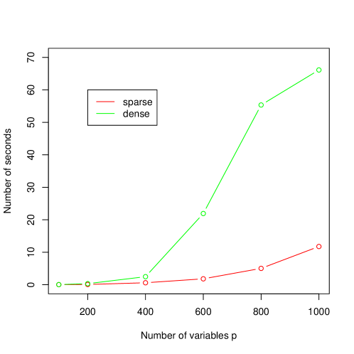
Figure 1 shows the number of CPU seconds required for the covariance lasso procedure, for problem sizes up to 1000. Even in the dense scenario, it solves a 1000 node problem ($\sim 500,000$ parameters) is about a minute.

Figure 1: Number of CPU seconds required for the covariance lasso procedure.

4 Analysis of cell signalling data

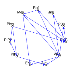
For illustration we analyze a flow cytometry dataset on $p=11$ proteins and $n=7466$ cells, from sachs2003. These authors fit a directed acyclic graph (DAG) to the data, producing the network in Figure 2.

Figure 2: Directed acylic graph from cell-signaling data, from sachs2003.

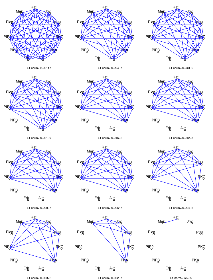
The result of applying the covariance Lasso to these data is shown in Figure 3, for 12 different values of the penalty parameter $\rho$.

Figure 3: Cell-signaling data: undirected graphs from covariance lasso with different values of the penalty parameter $\rho$.

There is moderate agreement between, for example, the graph for L1 norm $=0.00496$ and the DAG: the former has about half of the edges and non-edges that appear in the DAG. Figure 4 shows the lasso coefficients as a function of total $L_{1}$ norm of the coefficient vector.

Figure 4: Cell-signaling data: profile of coefficients as the total $L_{1}$ norm of the coefficient vector increases, that is, as $\rho$ decreases. Profiles for the largest coefficients are labeled with the corresponding pair of proteins.

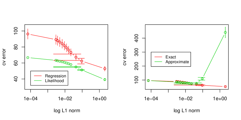
In the left panel of Figure 5 we tried two different kinds of 10-fold cross-validation for estimation of the parameter $\rho$. In the “Regression” approach, we fit the covariance-lasso to nine-tenths of the data, and used the penalized regression model for each protein to predict the value of that protein in the validation set. We then averaged the squared prediction errors over all 11 proteins. In the “Likelihood” approach, we again applied the covariance-lasso to nine-tenths of the data, and then evaluated the log-likelihood (1) over the validation set. The two cross-validation curves indicate that the unregularized model is the best, not surprising give the large number of observations and relatively small number of parameters. However we also see that the likelihood approach is far less variable than the regression method.

The right panel compares the cross-validated sum of squares of the exact covariance lasso approach to the Meinhausen-Buhlmann approximation. For lightly regularized models, the exact approach has a clear advantage.

Figure 5: Cell-signaling data. Left panel shows tenfold cross-validation using both Regression and Likelihood approaches (details in text). Right panel compares the regression sum of squares of the exact covariance lasso approach to the Meinhausen-Buhlmann approximation.

5 Discussion

We have presented a simple and fast algorithm for estimation of a sparse inverse covariance matrix using an $L_{1}$ penalty. It cycles through the variables, fitting a modified lasso regression to each variable in turn. The individual lasso problems are solved by coordinate descent.

The speed of this new procedure should facilitate the application of sparse inverse covariance procedures to large datasets involving thousands of parameters.

Fortran and R language routines for the proposed methods will be made freely available.

Acknowledgments

We thank the authors of BGA2007 for making their COVSEL program publicly available, and Larry Wasserman for helpful discussions. Friedman was partially supported by grant DMS-97-64431 from the National Science Foundation. Hastie was partially supported by grant DMS-0505676 from the National Science Foundation, and grant 2R01 CA 72028-07 from the National Institutes of Health. Tibshirani was partially supported by National Science Foundation Grant DMS-9971405 and National Institutes of Health Contract N01-HV-28183.