Anisotropic conductivity of disordered 2DEGs due to spin-orbit interactions

Abstract

We show that the disorder-averaged conductivity tensor of a disordered two-dimensional electron gas becomes anisotropic in the presence of both Rashba and Dresselhaus spin-orbit interactions (SOI). This anisotropy is a mesoscopic effect and vanishes with vanishing charge dephasing time. Using a diagrammatic approach including zero, one, and two-loop diagrams, we show that a consistent calculation needs to go beyond a Boltzmann equation approach. In the absence of charge dephasing and for zero frequency, a finite anisotropy $\sigma_{xy}\propto e^{2}/p_{\mathrm{F}}lh$ arises even for infinitesimal SOI, where $p_{\mathrm{F}}$ is the Fermi momentum and $l$ is the mean free path of an electron.

I Introduction

The interplay between spin and charge coherence effects in mesoscopic semiconductors produces interesting transport phenomena Awschalom et al. (2002); Zutic et al. (2004); Awschalom and Flatté (2007). They are based on the spin-orbit interaction (SOI), such as Rashba Rashba (2004) or Dresselhaus Dresselhaus (1955) type, which establishes a coupling between orbital and spin degrees of freedom of the electron.

One major effect of SOI on the conductivity of a disordered semiconductor is the sign reversal of weak localization effects. In this respect the influence of the SOI is similar to that of a magnetic field: it increases the conductivity. For Rashba and Dresselhaus SOI and in the presence of a magnetic field, this “weak antilocalization” effect has been studied in a number of papers Edelstein (1995); Skvortsov (1998); Zumbühl et al. (2002); Aleiner and Fal’ko (2001).

In the absence of magnetic fields, the Rashba SOI cannot violate isotropy of the energy spectrum. In this case, the conductivity tensor $\sigma_{\alpha\beta}$ is invariant under rotation of the coordinate system (CS) by $\pi/2$ and simultaneous sign change of the SOI. However, this sign is irrelevant for the conductivity (see Appendices), and thus $\sigma_{xx}=\sigma_{yy}$ and $\sigma_{xy}=-\sigma_{yx}$. In addition, due to time reversal invariance, $\sigma_{xy}=\sigma_{yx}$, so that $\sigma_{\alpha\beta}$ remains isotropic, i.e. $\sigma_{xy}=0$. This reasoning is no longer valid if rotational invariance of the spectrum is broken, e.g., by a Zeeman term which violates both time-reversal and rotational symmetries, leading to a finite anisotropy of the conductivity Schwab and Raimondi (2002).

A similar situation arises even without magnetic fields but when different types of SOI (such as Rashba and Dresselhaus) are present: the spectrum becomes anisotropic Schliemann and Loss (2003a) so that one can expect anisotropy of the conductivity. However, differently from before Schwab and Raimondi (2002), a system with only SOI remains invariant under time reversal. Nevertheless, we demonstrate below for a disordered two-dimensional electron gas (2DEG) that breaking of the rotation symmetry of the spectrum alone leads to an anisotropic conductivity.

Previous calculations in such a system were based on the Boltzmann equation Schliemann and Loss (2003a); Trushin and Schliemann (2007), with the outcome err that the conductivity does get enhanced by the SOI, but remains isotropic even when both Rashba and Dresselhaus terms are present.

However, in the presence of phase coherence, both for charge and spin, the standard Boltzmann approach is no longer sufficient. Indeed, this approach correctly describes contributions to $\sigma_{\alpha\beta}$ of the order of the Drude conductivity $\sigma_{\mathrm{D}}=e^{2}p_{\mathrm{F}}l/2h$, but, as is well-known, it already ’lacks accuracy’ to describe weak localization corrections $\sim\sigma_{\mathrm{D}}\hbar/p_{\mathrm{F}}l\ll\sigma_{\mathrm{D}}$ (here $p_{\mathrm{F}}$ and $l$ are Fermi momentum and mean free path of the electrons, resp.). We will see that the required accuracy for finding the anisotropy of the conductivity is even higher.

In the diagrammatic approach Abrikosov et al. (1975) used below, the leading contribution of a diagram to $\sigma_{\alpha\beta}$ is of the order of $\sigma_{\mathrm{D}}/(p_{\mathrm{F}}l/\hbar)^{n}$, where $n$ is the number of loops built by cooperon and diffuson lines in the diagram. (This is often called “loop expansion”.) Thus, the zeroth order is represented by two diagrams: the Drude “bubble” and the “vertex correction”, which are often referred to as “zero loop approximation” (ZLA) Chalaev and Loss (2005), indicating that these two diagrams have no loops made of cooperon and/or diffuson lines. One can easily check that, in leading order, these ZLA-diagrams are SOI-independent (the “bubble” gives $\sigma_{\mathrm{D}}$, while the “vertex correction” vanishes).

The SOI-dependent contribution to $\sigma_{\alpha\beta}$, coming from the ZLA, is isotropic and on the order $\sigma_{\mathrm{D}}/(p_{\mathrm{F}}l/\hbar)^{2}$. We will see that this is of the same order as contributions from diagrams with two loops. Thus, a consistent calculation (i.e. a systematic expansion in powers of $\hbar/p_{\mathrm{F}}l$) requires consideration of all the diagrams having zero, one, and two loops. Below we demonstrate that the isotropic conductivity, obtained from the Boltzmann equation Trushin and Schliemann (2007), corresponds to the ZLA. The inconsistency of the ZLA, and thus of the Boltzmann equation, has been pointed out before Chalaev and Loss (2005) in the context of the spin-Hall effect.

Taking all relevant diagrams systematically into account, we find that the conductivity has finite anisotropic components given by Eq. (16), or, when expressed in terms of charge and spin dephasing times, by Eq. (18). In the fully phase coherent limit, a finite anisotropy $\sigma_{xy}\propto e^{2}/2\pi p_{\mathrm{F}}l$ exists even for infinitesimal SOI.

The paper is organized as follows. In Sec. II, we calculate matrix elements of the diffuson at zero frequency; the result leads to the cancellation of the anomalous part of the velocity operator. Then, in Sec. III we realize that the (most commonly used) zero loop approximation (ZLA) gives an isotropic contribution to the conductivity tensor, similar to the result of the Boltzmann equation Trushin and Schliemann (2007). Then, we demonstrate that this ZLA result is incomplete in a given order $\hbar/p_{\mathrm{F}}l$, and higher order diagrams have to be considered. In Sec. IV we obtain the general form of the expansion for the anisotropic part of the conductivity. The main results are obtained in Sec. V, where we calculate the leading contribution to the anisotropy determined by two-loop diagrams and give estimates for real samples.

II Kubo Formula and Vertex Renormalization

Since the considered system is invariant under time reversal, $\sigma_{\alpha\beta}$ is symmetric and can thus be diagonalized. We will proceed with calculations in the CS rotated by $\pi/4$ with respect to the original one, where the 2D conductivity tensor is diagonal.

In linear-response theory, the conductivity tensor is given by the Kubo-Greenwood formula:

$$\sigma_{\alpha\beta}=\frac{e^{2}}{h}\overline{\mathop{\mathrm{Tr}}\left[{\hat{v}}_{\alpha}{\hat{G}}_{\mathrm{R}}{\hat{v}}_{\beta}{\hat{G}}_{\mathrm{A}}\right]},\quad\alpha,\beta=x,y,$$ (1)

where the overbar indicates averaging over the different disorder realizations, ${\hat{v}}_{\alpha}=\frac{i}{\hbar}[\hat{H},r_{\alpha}]$ is a component of the velocity operator, and ${\hat{G}}_{\mathrm{R}/A}=[E_{\mathrm{F}}-\hat{H}\pm i0]^{-1}$ with $E_{\mathrm{F}}$ being the Fermi energy (the derivation of (1) is analogous to the one in Chalaev and Loss (2005)). The Hamiltonian in our (rotated) CS reads

$$\begin{split}\hat{H}=&\frac{\hat{p}^{2}}{2m}+V_{s}+U({\bf r}),\\ V_{s}=&(a-b){{\tilde{\sigma}}}_{1}\hat{p}_{y}-(a+b){{\tilde{\sigma}}}_{2}\hat{p}_{x},\end{split}$$ (2)

where $a$ and $b$ are the amplitudes of Rashba and Dresselhaus SOI, ${{\tilde{\sigma}}}_{1,2}$ are expressed in terms of Pauli matrices as ${{\tilde{\sigma}}}_{1,2}=(\sigma_{2}\pm\sigma_{1})/\sqrt{2}$, and $U({\bf r})$ is a short-range impurity potential, $\overline{U({\bf r})U({\bf r}\,^{\prime})}=\hbar^{3}(m\tau)^{-1}\delta({\bf r}-{\bf r}\,^{\prime})$ (we use notations similar to Chalaev and Loss (2005)). The conductivity (1) is not affected by a simultaneous sign-reversal of $a$ and $b$; thus, without loss of generality, we can assume that $a+b>0$.

In the absence of SOI, the disorder-averaged retarded Green function (GF) is given by Abrikosov et al. (1975)

$$G_{\mathrm{R}}^{(0)}=\left[G_{\mathrm{A}}^{(0)}\right]^{\dagger}=\sigma_{0}\left[E_{\mathrm{F}}-\frac{p^{2}}{2m}+\frac{i\hbar}{2\tau}\right]^{-1},$$ (3)

where $\sigma_{0}$ is the $2\times 2$ unity matrix (due to spin degrees of freedom), and $\tau$ is the mean time between collisions of an electron off impurities. The presence of the SOI modifies (3) as follows:

$$G_{\mathrm{R}}=G_{\mathrm{R}}^{(0)}\sum_{n\geq 0}\left(V_{s}G_{\mathrm{R}}^{(0)}\right)^{n}=\left[{\left(G_{\mathrm{R}}^{(0)}\right)^{-1}-V_{s}}\right]^{-1}.$$ (4)

The disorder-averaging of (1) produces an infinite number of diagrams classified according to the number of loops composed by cooperon and diffuson lines. Each of these diagrams contains two velocity vertices, both exc being renormalized by the vertex correction Chalaev and Loss (2005), so that their “anomalous” (i.e., SOI-dependent) part cancels:

$$\begin{split}\hat{{\bf v}}=&\frac{\hat{{\bf p}}}{m}+\begin{pmatrix}-(a+b){{\tilde{\sigma}}}_{2}\\ (a-b){{\tilde{\sigma}}}_{1}\end{pmatrix},\\ {\hat{\tilde{v}}}_{\alpha}=&{\hat{v}}_{\alpha}+\sum_{\gamma=1}^{3}{{\tilde{\sigma}}}_{\gamma}D^{\gamma\gamma}\mathop{\mathrm{Tr}}_{{\bf p}}\left[{{\tilde{\sigma}}}_{\gamma}G_{\mathrm{R}}({\bf p}){\hat{v}}_{\alpha}G_{\mathrm{A}}({\bf p})\right]=\frac{{\hat{p}}_{\alpha}}{m},\end{split}$$ (5)

where

$$\begin{split}(&D^{11},D^{22},D^{33})=\\ =&\frac{\hbar}{m\tau}\left(1+\frac{1+K}{(x_{a}+x_{b})^{2}},1+\frac{1+K}{(x_{a}-x_{b})^{2}},\frac{K}{K-1}\right)\end{split}$$ (6)

are the components of the diffuson at zero momentum, $K=\sqrt{[1+(x_{a}+x_{b})^{2}][1+(x_{a}-x_{b})^{2}]}$, and we have introduced dimensionless Rashba and Dresselhaus amplitudes, $x_{a}=2p_{\mathrm{F}}a\tau/\hbar$ and $x_{b}=2p_{\mathrm{F}}b\tau/\hbar$. [Note that (5) is not exact at finite frequency.]

III The zero-loop approximation

In the ZLA, the conductivity is given by two diagrams – the “bubble” and the “vertex correction” Chalaev and Loss (2005), which, when being summed, result in the following SOI-dependent correction to the conductivity foo (a):

$$\begin{split}\delta\sigma_{\alpha\beta}=\frac{e^{2}}{h}\mathop{\mathrm{Tr}}_{{\bf p}}\big{[}{\hat{\tilde{v}}}_{\alpha}G_{\mathrm{R}}({\bf p}){\hat{v}}_{\beta}G_{\mathrm{A}}({\bf p})&\\ -{\hat{\tilde{v}}}_{\alpha}G_{\mathrm{R}}^{(0)}({\bf p}){\hat{v}}_{\beta}G_{\mathrm{A}}^{(0)}({\bf p})\big{]}=\frac{e^{2}}{h}&\frac{x_{a}^{2}+x_{b}^{2}}{2p_{\mathrm{F}}l/\hbar}\begin{pmatrix}1&0\\ 0&1\end{pmatrix},\end{split}$$ (7)

where $G_{\mathrm{R}/A}^{(0)}$ is given in (3) and $\mathop{\mathrm{Tr}}_{{\bf p}}\equiv\int\frac{\mathrm{d}^{2}p}{(2\pi)^{2}}$. The result (7) has been confirmed (up to a missing factor $4$) in Trushin and Schliemann (2007) by using the Boltzmann equation approach; so one can conclude that ZLA corresponds to the result of the Boltzmann equation with the simplest (and most common) form of the collision integral. However, since (7) is of the order of $\sigma_{\mathrm{D}}/(p_{\mathrm{F}}l/\hbar)^{2}\ll\sigma_{\mathrm{D}}$, the calculation in the ZLA (as well as the Boltzmann equation Trushin and Schliemann (2007)) is incomplete.

To re-enforce this point, let us consider the special case when $a=\pm b$. Then, all four operators under the $\mathop{\mathrm{Tr}}$ in (1) can be diagonalized by a momentum-independent unitary transformation, and one can see that the SOI-dependent correction to the conductivity vanishes already before the disorder averaging (see Appendix B). This is just further evidence that the expression (7) is incomplete; other contributions must be taken into account to cancel it when $a=\pm b$.

IV Contribution of higher orders

According to the loop expansion Chalaev and Loss (2005), diagrams having one (weak localization Edelstein (1995); Skvortsov (1998)) and two loops may produce contributions to $\sigma_{\alpha\beta}$ of the same or even larger order than (7). There exist one diagram with one loop and nine diagrams with two loops.

From now on we assume that the SOI and the spectrum anisotropy due to it are small:

$$x=\sqrt{x_{a}^{2}+x_{b}^{2}}\ll 1,\ \delta=\frac{2ab}{a^{2}+b^{2}},\ |\delta|\ll 1.$$ (8)

We have chosen $x$ and $\delta$ as expansion parameters because they provide a uniform expansion for the conductivity (9).

The anisotropic part of the conductivity tensor is given by an expansion in inverse powers of $p_{\mathrm{F}}l/\hbar\gg 1$:

$$\sigma_{xx}-\sigma_{yy}=2\frac{e^{2}}{h}\sum_{r\geq 0}\frac{1}{(p_{\mathrm{F}}l/\hbar)^{r-1}}\sum_{m,n\geq 0}S_{mn}^{r}x^{m}\delta^{2n+1},$$ (9)

where we used (41).

By calculating the conductivity in the ZLA we have checked that $S_{mn}^{0}=0$ $\forall m,n$. From the properties of the weak localization (WL) diagram (which is the only one that could contribute to $S_{00}^{1}$), one can easily show that $S_{00}^{1}=0$ as well. Thus, in the limit when $p_{\mathrm{F}}l\delta^{2}/\hbar<1$, the leading anisotropic contribution is given by the term $\propto S_{00}^{2}$ in the expansion (9), which we calculate below.

V Diagrams with two loops

We have checked that, like the ZLA, the WL diagram does not contribute to $S_{00}^{2}$. The same is true for 6 (out of 9) two-loop diagrams. The remaining 3 diagrams, which we calculate below, are depicted in Fig. 1.

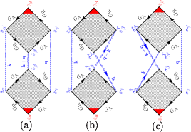
Figure 1: Three relevant two-loop diagrams (out of nine) for the conductivity tensor $\sigma_{\alpha\beta}$. The matrix vertices ${\tilde{\sigma}}$ and $\bar{\sigma}$ are written assuming clockwise (in lower Hikami boxes) and counterclockwise (in upper Hikami boxes) direction of writing traces ($\mathop{\mathrm{Tr}}$). Each diagram contains small-momentum singularities, which cancel each other in accordance with the theorem from Vollhardt and Wölfle (1980).

In addition to the figure caption, some comments are necessary. Straight bold lines represent averaged retarded and advanced GFs, given by (4) and its Hermitian conjugate. The squares built of GFs are Hikami boxes Gor’kov et al. (1979). A Hikami box (HB) is given by three contributions, cf. Chalaev and Loss (2005): one empty box and two boxes with an impurity line inside. Wavy lines with (without) arrows represent cooperons (diffusons).

Using the identity $\sum_{\alpha=0}^{3}{\tilde{\sigma}}^{s_{1}s_{3}}_{\alpha}{{\tilde{\sigma}}}^{s_{4}s_{2}}_{\alpha}=2\delta_{s_{1}s_{2}}\delta_{s_{3}s_{4}}$, we write the diffuson in the basis of matrices ${\tilde{\sigma}}$ as $D_{{\bf q}}=\frac{\hbar}{2m\tau}\left[\mathds{1}-{\tilde{X}}_{D}({\bf q}\,)\right]^{-1}$, where $\mathds{1}$ is a $4\times 4$ unity matrix, and

$${\tilde{X}}_{D}^{\alpha\beta}({\bf q}\,)=\frac{\hbar}{2m\tau}\mathop{\mathrm{Tr}}_{{\bf p}}[{\tilde{\sigma}}_{\alpha}G^{E}_{\mathrm{R}}({\bf p}\,){\tilde{\sigma}}_{\beta}G^{E-\omega}_{\mathrm{A}}({\bf p}-{\bf q}\,)].$$ (10)

For cooperon lines in diagrams 1b and 1c, we use the expression $C_{{\bf q}}=\frac{\hbar}{2m\tau}\left[\mathds{1}-{{\bar{X}}}_{C}({\bf q}\,)\right]^{-1}$, so that the cooperon series starts with one disorder line. Thus each diagram in Fig. 1 contains an extra contribution, belonging to the WL diagram. However, this contribution can affect $S_{mn}^{r}$ in (9) only for $m\geq 1$, so we neglect it. To make the similarity between diffuson and cooperon more evident, we use a different matrix basis for the cooperon:

$${{\bar{X}}}_{C}^{\alpha\beta}({\bf q}\,)=\frac{\hbar}{2m\tau}\mathop{\mathrm{Tr}}_{{\bf p}}\{{\bar{\sigma}}_{\alpha}G^{E}_{\mathrm{R}}({\bf p}\,){\bar{\sigma}}^{\dagger}_{\beta}[G^{E-\omega}_{\mathrm{A}}({\bf q}-{\bf p}\,)]^{T}\},$$ (11)

where ${\bar{\sigma}}_{\alpha}=\sigma_{2}{{\tilde{\sigma}}}_{\alpha}$, and $\sum_{\alpha=0}^{3}{{\bar{\sigma}}}^{s_{1}s_{3}}_{\alpha}\left({{\bar{\sigma}}}_{\alpha}^{\dagger}\right)^{s_{4}s_{2}}=2\delta_{s_{1}s_{2}}\delta_{s_{3}s_{4}}$. Because of the time-reversal symmetry, $\sigma_{2}G_{\mathrm{A}}^{T}(-{\bf p}\,)\sigma_{2}=G_{\mathrm{A}}({\bf p}\,)$, so that ${{\bar{X}}}_{C}({\bf q}\,)={\tilde{X}}_{D}({\bf q}\,)$ and $C_{{\bf q}}=D_{{\bf q}}$. Thus the expressions for cooperon/diffuson lines are the same for all diagrams in Fig. 1, and the same is true for the lower HBs $L_{\alpha\beta\gamma}$. As a consequence, the sum of the three diagrams is equal to the diagram in Fig. 1a with a “renormalized” upper HB $R_{\alpha^{\prime}\beta^{\prime}\gamma^{\prime}}$ (given by the sum of upper HBs of all three diagrams), see the expression for $\delta\sigma_{xx}^{\mathrm{II}}$ in (12).

Due to (41) the anisotropy of the conductivity is given by $\sigma_{xx}(a,b)-\sigma_{yy}(a,b)=\sigma_{xx}(a,b)-\sigma_{xx}(a,-b)$, so it suffices to calculate only the SOI-dependent part of $\sigma_{xx}$. The total contribution of the diagrams in Fig. 1 is an integral from the product of two HBs ($L$ and $R$) and three diffusons ($D$):

$$\begin{split}\delta\sigma_{xx}^{\mathrm{II}}=\frac{e^{2}}{h}\int\frac{\mathrm{d}^{2}k}{(2\pi)^{2}}\int\frac{\mathrm{d}^{2}q}{(2\pi)^{2}}\sum_{\alpha,\beta,\gamma=0}^{3}\\ \sum_{\alpha^{\prime},\beta^{\prime},\gamma^{\prime}=0}^{3}L_{\alpha\beta\gamma}D^{\alpha\alpha^{\prime}}_{{\bf k}}D^{\beta^{\prime}\beta}_{{\bf k}+{\bf q}}D^{\gamma\gamma^{\prime}}_{{\bf q}}R_{\alpha^{\prime}\beta^{\prime}\gamma^{\prime}}.\end{split}$$ (12)

First, we evaluate (12) for zero frequency $\omega=0$. In the absence of SOI, the HBs are given by

$$\begin{split}L^{\mathrm{0}}_{\alpha\beta\gamma}=-2i\frac{p_{\mathrm{F}}l\tau^{3}}{\hbar^{4}}(k_{x}+q_{x})\mathop{\mathrm{Tr}}[{\tilde{\sigma}}_{\alpha}{\tilde{\sigma}}_{\beta}{\tilde{\sigma}}_{\gamma}],\\ R^{0}_{\alpha\beta\gamma}=-4i\frac{p_{\mathrm{F}}l\tau^{3}}{\hbar^{4}}\big{\{}(1-\delta_{\beta 0})(k_{x}\delta_{\alpha 0}\delta_{\beta\gamma}+q_{x}\delta_{\gamma 0}\delta_{\alpha\beta})+\\ (k_{x}+q_{x})(1-\delta_{\alpha 0})\big{[}\delta_{\beta 0}\delta_{\alpha\gamma}+i\epsilon_{\alpha\beta\gamma}(1-\delta_{\beta 0})(1-\delta_{\gamma 0})\big{]}\big{\}},\end{split}$$ (13)

where $\epsilon_{\alpha\beta\gamma}$ is the Levi-Cività tensor. The SOI-dependent part of the HBs is shown in Tab. 1. Due to SOI, additional nonzero matrix elements appear, $L^{\mathrm{s}}_{\alpha\beta\gamma}$ and $R^{\mathrm{s}}_{\alpha^{\prime}\beta^{\prime}\gamma^{\prime}}$, so that $L_{\alpha\beta\gamma}=L^{\mathrm{0}}_{\alpha\beta\gamma}+L^{\mathrm{s}}_{\alpha\beta\gamma}$ and $R_{\alpha^{\prime}\beta^{\prime}\gamma^{\prime}}=R^{0}_{\alpha^{\prime}\beta^{\prime}\gamma^{\prime}}+R^{\mathrm{s}}_{\alpha^{\prime}\beta^{\prime}\gamma^{\prime}}$, see Tab. 1.

$\alpha$	$0$	$0$	$1$	$1$	$2$	$2$	$3$	$3$
$\beta$	$1$	$3$	$1$	$3$	$1$	$3$	$1$	$3$
$\gamma$	$3$	$1$	$2$	$0$	$1$	$3$	$0$	$2$
$\frac{L^{\mathrm{s}}_{\alpha\beta\gamma}\hbar^{3}}{2p_{\mathrm{F}}\tau^{3}(x_{a}+x_{b})}$	$-1$	$1$	$i$	$1$	$-i$	$-i$	$-1$	$i$
$\frac{R^{\mathrm{s}}_{\alpha\beta\gamma}\hbar^{3}}{2p_{\mathrm{F}}\tau^{3}(x_{a}+x_{b})}$	$0$	$0$	$-2i$	$0$	$2i$	$2i$	$0$	$-2i$

Table 1: The first order SOI-correction to the Hikami boxes ($L^{\mathrm{s}}_{\alpha\beta\gamma}$ and $R^{\mathrm{s}}_{\alpha^{\prime}\beta^{\prime}\gamma^{\prime}}$). Other matrix elements vanish. Each of three upper Hikami boxes has non-zero elements with $\alpha=0$ or $\gamma=0$, so that each diagram diverges at ${\bf k}\to 0$ or at ${\bf q}\to 0$; however, these elements cancel each other (note the zeroes in the last row), so that the complete expression for the conductivity converges.

Like the HBs, ${\tilde{X}}_{D}$ defined in (10) can be split into a main part and a SOI-dependent correction, which (for $\omega=0$) are given by ${\tilde{X}}_{D}^{\mathrm{0}}({\bf q}\,)=\left(1-l^{2}q^{2}/2\hbar^{2}\right)\mathds{1}$ and

$${\tilde{X}}_{D}^{\mathrm{s}}({\bf q}\,)=$$

$$\begin{pmatrix}0&0&0&0\\ 0&\frac{(x_{a}+x_{b})^{2}}{2}&0&-i\frac{q_{x}l}{\hbar}(x_{a}+x_{b})\\ 0&0&\frac{(x_{a}-x_{b})^{2}}{2}&-i\frac{q_{y}l}{\hbar}(x_{a}-x_{b})\\ 0&i\frac{q_{x}l}{\hbar}(x_{a}+x_{b})&i\frac{q_{y}l}{\hbar}(x_{a}-x_{b})&x_{a}^{2}+x_{b}^{2}\end{pmatrix}.$$

Hence the diffusons in (12) are given by

$$D_{{\bf q}}=\frac{\hbar}{2m\tau}\left[\mathds{1}-{\tilde{X}}_{D}^{\mathrm{0}}({\bf q}\,)-{\tilde{X}}_{D}^{\mathrm{s}}({\bf q}\,)\right]^{-1},$$ (15)

where ${\tilde{X}}_{D}^{\mathrm{s}}$ is written in (V).

Two angular integrations in (12) were performed analytically using maxima max (the result is too lengthy to be presented here), while the integrations over $k$, $q$ were done numerically, using quadpack qua .

Finally, we obtain the following result for the anisotropy of the conductivity at $\omega=0$,

$$\begin{split}\delta\sigma=2\delta\sigma_{xx}^{\mathrm{II}}=\sigma_{xx}-\sigma_{yy}=2S^{2}_{00}\frac{2x_{a}x_{b}}{x_{a}^{2}+x_{b}^{2}}\frac{e^{2}}{2\pi}\frac{1}{p_{\mathrm{F}}l},\\ S^{2}_{00}=-5.6\times 10^{-3},\quad 2x_{a}x_{b}\ll x_{a}^{2}+x_{b}^{2}\ll 1.\end{split}$$ (16)

The result (16) has been obtained in the CS rotated by $\pi/4$, where the sum of Rashba and Dresselhaus terms are given by $V_{s}$ in (2). In the original coordinates, the conductivity has equal diagonal elements, and equal non-zero off-diagonal elements $\sigma_{xy}=\sigma_{yx}=\delta\sigma/2$.

The correction (16) depends non-analytically on the SOI in the vicinity of $x_{a}^{2}+x_{b}^{2}=0$, so that at $\omega=0$ even an infinitesimally small SOI can produce a finite anisotropy. This is not entirely surprising, since a similar non-analyticity is also seen to emerge in the weak-localization correction with Rashba SOI only and for vanishing dephasing (see, e.g., Eq. (17) in Ref. Skvortsov (1998)).

The analyticity is restored at finite frequency:

$$\begin{split}\delta\sigma=-2\cdot 0.25\cdot\frac{-2i\omega\tau\cdot 2x_{a}x_{b}}{(x_{a}^{2}+x_{b}^{2}-2i\omega\tau)^{2}}\frac{e^{2}}{2\pi}\frac{1}{p_{\mathrm{F}}l},\\ 2x_{a}x_{b}\ll x_{a}^{2}+x_{b}^{2}\ll\omega\tau\ll 1.\end{split}$$ (17)

To account for charge dephasing effects, we follow standard procedure Altshuler et al. (1982) and substitute $-i\omega\tau\to\tau/\tau_{\phi}$, with $\tau_{\phi}$ the charge dephasing time (e.g., due to electron-electron interactions). In addition, one can express the SOI parameters in terms of spin dephasing times of Dyakonov-Perel type Averkiev et al. (2002), allowing us to rewrite (16), (17) as

$$\delta\sigma=\left\{\begin{aligned} 5.6\times 10^{-3}\cdot\frac{\tau_{-}-\tau_{+}}{\tau_{-}+\tau_{+}}\frac{e^{2}}{2\pi}\frac{1}{E_{\mathrm{F}}\tau},\quad\tau_{\pm}\ll\tau_{\phi},\\ 0.13\cdot\left(\frac{\tau_{\phi}}{\tau_{+}}-\frac{\tau_{\phi}}{\tau_{-}}\right)\frac{e^{2}}{2\pi}\frac{1}{E_{\mathrm{F}}\tau},\quad\tau_{\phi}\ll\tau_{\pm},\end{aligned}\right.$$ (18)

whereAverkiev et al. (2002) $2\tau/\tau_{\pm}=(x_{a}\mp x_{b})^{2}$. In a diffusive semiconductor (e.g., GaAs) for $p_{\mathrm{F}}l/\hbar=5$ we estimate $\delta\sigma\lesssim 5\cdot 10^{-4}\sigma_{D}$ in case $\tau_{\pm}\ll\tau_{\phi}$ and $\delta\sigma\lesssim 10^{-2}\sigma_{D}$ in the opposite case $\tau_{\pm}\gg\tau_{\phi}$.

Thus, in a system with finite dephasing time $\tau_{\phi}$, the anisotropic conductivity (18) is analytic in $\tau_{\pm}$. However, in a fully phase-coherent system with $\tau_{\phi}=\infty$ (which is commonly predicted at zero temperature), the conductivity tensor depends non-analytically on the SOI.

VI Conclusion

The combination of Rashba and Dresselhaus SOI leads to anisotropy in the energy spectrum, which, in turn, leads to anisotropy in the conductivity of a disordered 2DEG. This anisotropy, being due to phase coherence of charge and spin, comes from two-loop diagrams in the perturbative approach, while it is absent in the Boltzmann equation approach. In the limit of full phase coherence, the system “jumps” from isotropic to anisotropic state for infinitesimally small SOIs.

We are grateful to B. Altshuler, M. Duckheim, A. Khaetskii, and E. Rashba for helpful discussions. We acknowledge financial support from the Swiss NSF and the NCCR Nanoscience.

Appendix A Conductivity for pure-Rashba or pure-Dresselhaus SOI

Using the time-reversal invariance we argued in the Introduction (Sec. I) that the conductivity tensor is isotropic in case of a pure-Rashba SOI. Here we demonstrate this isotropy for both pure-Rashba and pure-Dresselhaus cases using only rotation symmetry of the disorder-free part of the Hamiltonian.

The conductivity tensor in the rotated CS is connected with its value in the original CS through the transformation

$$\sigma_{\alpha\beta}\to(R_{\phi}\sigma R_{\phi}^{-1})_{\alpha\beta},$$ (19)

where $R_{\phi}$ is a 3D-rotation matrix in the $(x,y)$-plane by angle $\phi$. In this section, we prove that when $a=0$ or $b=0$, the conductivity tensor is invariant with respect to rotations in the $(x,y)$-plane; together with the requirement (19) this means that $\sigma_{\alpha\beta}$ is isotropic.

We define matrices

$$T=\frac{1}{\sqrt{2}}\begin{pmatrix}0&1+i\cr 1-i&0\end{pmatrix},\quad C=\begin{pmatrix}0&-1&0\cr-1&0&0\cr 0&0&-1\end{pmatrix}.$$ (20)

The Hamiltonian (2) can be rewritten as

$$\hat{H}=\frac{{\hat{p}}^{2}}{2m}+aV_{R}+bV_{D}+U({\bf r}),$$ (21)

where (in the original -unrotated- CS)

$$V_{R}={{\bf e}}_{z}\cdot\left[\boldsymbol{\sigma}\times{\hat{{\bf p}}}\right],\quad V_{D}={{\bf e}}_{z}\cdot\left[C\boldsymbol{\sigma}\times{\hat{{\bf p}}}\right],$$ (22)

$\boldsymbol{\sigma}\equiv(\sigma_{1},\sigma_{2},\sigma_{3})$, and ${{\bf e}}_{z}$ is the unit vector along the $z$-axis. A rotation of the CS corresponds to the transformation of coordinates, momenta and spins according to

$$(\sigma_{0},\boldsymbol{\sigma})\to(\sigma_{0},R_{\phi}\boldsymbol{\sigma}),\quad\hat{{\bf p}}\to R_{\phi}\hat{{\bf p}},\quad{\bf r}\to R_{\phi}{\bf r}.$$ (23)

We note that $V_{R}$ is invariant under the transformation (23):

$$V_{R}={{\bf e}}_{z}\cdot\left[R_{\phi}\boldsymbol{\sigma}\times R_{\phi}{\hat{{\bf p}}}\right]=\begin{pmatrix}0&{\hat{p}}_{y}+i{\hat{p}}_{x}\cr{\hat{p}}_{y}-i{\hat{p}}_{x}&0\end{pmatrix}.$$ (24)

The same invariance holds for the (disorder-averaged) pure-Rashba Green functions $G_{\mathrm{R}/A}^{Ra}$. Thus, the contribution to the conductivity tensor from the (simplest) bubble diagram Chalaev and Loss (2005)

$$\begin{split}\sigma^{Ra}_{\alpha\beta}=&\frac{e^{2}}{h}\mathop{\mathrm{Tr}}_{{\bf p}}\mathop{\mathrm{Tr}}_{\mathrm{spin}}\left[{\hat{v}}_{\alpha}^{Ra}G_{\mathrm{R}}^{Ra}{\hat{v}}_{\beta}^{Ra}G_{\mathrm{A}}^{Ra}\right],\\ {\hat{v}}_{\alpha}^{Ra}=&\frac{i}{\hbar}\left[\frac{{\hat{p}}^{2}}{2m}+aV_{R},r_{\alpha}\right]\end{split}$$ (25)

is invariant under the rotation (23), and hence isotropic [due to 19)] in a pure-Rashba SOI system. As an example of a higher-loop correction, let us consider the two-loop contribution (12). The symmetry transformation (23) will affect (12) twofold: (i) as a momentum rotation ${\bf k},{\bf q}\to R_{\phi}{\bf k},R_{\phi}{\bf q}$ and (ii) through a different set of Pauli matrices $(\sigma_{0},\boldsymbol{\sigma}^{\prime})=(\sigma_{0},R_{\phi}\boldsymbol{\sigma})$ in the calculation of diffusons and Hikami boxes. The rotation of momenta can be absorbed by a variable change in the integration. Then, the result of the calculation does not depend on the choice of Pauli matrices, once they obey standard commutation relations. Since the new set $(\sigma_{0},\boldsymbol{\sigma}^{\prime})$ is connected through a unitary transformation with the standard one, $(\sigma_{0},\boldsymbol{\sigma})$ the commutation relations are preserved so that (12) is invariant under the transformation (23). Thus, the two-loop contribution (12) does not change when the CS is rotated in the $(x,y)$-plane. Analogously, the contribution from any other diagram is invariant under the transformation (23) in case when $b=0$, so that [due to 19)] the pure-Rashba conductivity tensor is isotropic.

Let us now demonstrate that also in case of pure-Dresselhaus SOI the conductivity is isotropic. The Dresselhaus SOI can be transformed into Rashba SOI by a unitary transformation: $V_{D}=T^{\dagger}V_{R}T$; the same is true for the pure-Dresselhaus velocity operator: ${\hat{v}}_{\alpha}^{Db}=\frac{i}{\hbar}\left[\frac{{\hat{p}}^{2}}{2m}+bV_{D},r_{\alpha}\right]=T^{\dagger}{\hat{v}}_{\alpha}^{Rb}T$. So, one can transform the pure-Dresselhaus conductivity tensor into the pure-Rashba one:

$$\begin{split}\sigma^{Db}_{\alpha\beta}=&\frac{e^{2}}{h}\mathop{\mathrm{Tr}}\left[{\hat{v}}_{\alpha}^{Db}G_{\mathrm{R}}^{Db}{\hat{v}}_{\beta}^{Db}G_{\mathrm{A}}^{Db}\right]\\ =&\frac{e^{2}}{h}\mathop{\mathrm{Tr}}\left[T^{\dagger}{\hat{v}}_{\alpha}^{Rb}TT^{\dagger}G_{\mathrm{R}}^{Rb}TT^{\dagger}{\hat{v}}_{\beta}^{Rb}TT^{\dagger}G_{\mathrm{A}}^{Rb}T\right],\end{split}$$ (26)

so that $\sigma^{Ra}_{\alpha\beta}=\sigma^{Da}_{\alpha\beta}$. With (26) we proved this statement for the (simplest) bubble diagram Chalaev and Loss (2005); it can be generalized to higher-loop corrections analogously to the pure-Rashba case [see (25) above]. We conclude that the disorder-averaged conductivity tensor is isotropic in a system with either pure Rashba or pure Dresselhaus SOI.

Appendix B Conductivity in case when $a=\pm b$

The case, when the moduli of Rashba and Dresselhaus SOI amplitudes are equal, is special Schliemann et al. (2003); Schliemann and Loss (2003b); Chalaev and Loss (2005). Both Hamiltonian and velocity operators can then be diagonalized in spin space by unitary transformations: for $a=b$, up to an irrelevant constant (in the rotated CS)

$$U_{1}\hat{H}U_{1}^{\dagger}=\frac{m}{2}\left[\left(\frac{{\hat{p}}_{x}}{m}-2a\sigma_{3}\right)^{2}+\frac{{\hat{p}}_{y}^{2}}{m^{2}}\right]+U({\bf r}),$$ (27)

and

$$U_{1}\hat{{\bf v}}U_{1}^{\dagger}=\begin{pmatrix}\frac{{\hat{p}}_{x}}{m}-2a\sigma_{3}\\ \frac{{\hat{p}}_{y}}{m}\end{pmatrix},$$ (28)

where the transformation matrix is given by

$$U_{1}=(U_{1}^{\dagger})^{-1}=\frac{1}{\sqrt{2}}\begin{pmatrix}1&-e^{i\pi/4}\\ 1&e^{i\pi/4}\end{pmatrix}.$$ (29)

For $a=-b$,

$$U_{2}\hat{H}U_{2}^{\dagger}=\frac{m}{2}\left[\left(\frac{{\hat{p}}_{y}}{m}+2b\sigma_{3}\right)^{2}+\frac{{\hat{p}}_{x}^{2}}{m^{2}}\right]+U({\bf r}),$$ (30)

and

$$U_{2}\hat{{\bf v}}U_{2}^{\dagger}=\begin{pmatrix}\frac{{\hat{p}}_{x}}{m}\\ \frac{{\hat{p}}_{y}}{m}+2b\sigma_{3}\end{pmatrix},$$ (31)

with

$$U_{2}=(U_{2}^{\dagger})^{-1}=\frac{1}{\sqrt{2}}\begin{pmatrix}1&-e^{-i\pi/4}\\ 1&e^{-i\pi/4}\end{pmatrix}.$$ (32)

Let us denote the (unaveraged) Green functions without SOI ($a=b=0$) as ${\hat{g}}_{\mathrm{r/a}}$.

With $U_{1,2}$ from (29) and (32) we diagonalize all operators under the trace $\mathop{\mathrm{Tr}}$ in the conductivity expressions below. Then the spin part of $\mathop{\mathrm{Tr}}\equiv\mathop{\mathrm{Tr}}_{\mathrm{spin}}\mathop{\mathrm{Tr}}_{{\bf p}}$ splits into two terms. For $a=b$,

$$\begin{split}&a=b\Rightarrow\mathop{\mathrm{Tr}}_{{\bf p}}\mathop{\mathrm{Tr}}_{\mathrm{spin}}\left[{\hat{v}}_{x}{\hat{G}}_{\mathrm{R}}{\hat{v}}_{x}{\hat{G}}_{\mathrm{A}}\right]\\ &=\mathop{\mathrm{Tr}}_{{\bf p}}\mathop{\mathrm{Tr}}_{\mathrm{spin}}\left[U_{1}{\hat{v}}_{x}U_{1}^{\dagger}U_{1}{\hat{G}}_{\mathrm{R}}U_{1}^{\dagger}U_{1}{\hat{v}}_{x}U_{1}^{\dagger}U_{1}{\hat{G}}_{\mathrm{A}}U_{1}^{\dagger}\right]\\ &=\mathop{\mathrm{Tr}}_{{\bf p}}\left\{\left[\frac{{\hat{p}}_{x}}{m}{\hat{g}}_{\mathrm{r}}\frac{{\hat{p}}_{x}}{m}{\hat{g}}_{\mathrm{a}}\right]\left|\vphantom{\Big{[}}\right._{{\hat{p}}_{x}\to{\hat{p}}_{x}-2ma}+\left[\frac{{\hat{p}}_{x}}{m}{\hat{g}}_{\mathrm{r}}\frac{{\hat{p}}_{x}}{m}{\hat{g}}_{\mathrm{a}}\right]\left|\vphantom{\Big{[}}\right._{{\hat{p}}_{x}\to{\hat{p}}_{x}+2ma}\right\}\\ &=2\mathop{\mathrm{Tr}}_{{\bf p}}\left[\frac{{\hat{p}}_{x}}{m}{\hat{g}}_{\mathrm{r}}\frac{{\hat{p}}_{x}}{m}{\hat{g}}_{\mathrm{a}}\right]=2\mathop{\mathrm{Tr}}_{{\bf p}}\left[\frac{{\hat{p}}_{y}}{m}{\hat{g}}_{\mathrm{r}}\frac{{\hat{p}}_{y}}{m}{\hat{g}}_{\mathrm{a}}\right],\\ \end{split}$$ (33)

and for $a=-b$,

$$\begin{split}&a=-b\Rightarrow\mathop{\mathrm{Tr}}_{{\bf p}}\mathop{\mathrm{Tr}}_{\mathrm{spin}}\left[{\hat{v}}_{y}{\hat{G}}_{\mathrm{R}}{\hat{v}}_{y}{\hat{G}}_{\mathrm{A}}\right]\\ &=\mathop{\mathrm{Tr}}_{{\bf p}}\mathop{\mathrm{Tr}}_{\mathrm{spin}}\left[U_{2}{\hat{v}}_{y}U_{2}^{\dagger}U_{2}{\hat{G}}_{\mathrm{R}}U_{2}^{\dagger}U_{2}{\hat{v}}_{y}U_{2}^{\dagger}U_{2}{\hat{G}}_{\mathrm{A}}U_{2}^{\dagger}\right]\\ &=\mathop{\mathrm{Tr}}_{{\bf p}}\left\{\left[\frac{{\hat{p}}_{y}}{m}{\hat{g}}_{\mathrm{r}}\frac{{\hat{p}}_{y}}{m}{\hat{g}}_{\mathrm{a}}\right]\left|\vphantom{\Big{[}}\right._{{\hat{p}}_{y}\to{\hat{p}}_{y}-2mb}+\left[\frac{{\hat{p}}_{y}}{m}{\hat{g}}_{\mathrm{r}}\frac{{\hat{p}}_{y}}{m}{\hat{g}}_{\mathrm{a}}\right]\left|\vphantom{\Big{[}}\right._{{\hat{p}}_{y}\to{\hat{p}}_{y}+2mb}\right\}\\ &=2\mathop{\mathrm{Tr}}_{{\bf p}}\left[\frac{{\hat{p}}_{y}}{m}{\hat{g}}_{\mathrm{r}}\frac{{\hat{p}}_{y}}{m}{\hat{g}}_{\mathrm{a}}\right]=2\mathop{\mathrm{Tr}}_{{\bf p}}\left[\frac{{\hat{p}}_{x}}{m}{\hat{g}}_{\mathrm{r}}\frac{{\hat{p}}_{x}}{m}{\hat{g}}_{\mathrm{a}}\right].\end{split}$$ (34)

Thus, we see that in the rotated CS $\sigma_{\alpha\alpha}$ are the same as in the absence of SOI for $a=\pm b$:

$$a=\pm b\quad\Longrightarrow\quad\sigma_{xx}=\sigma_{yy}=\sigma_{xx}(a=b=0).$$ (35)

This proves that the ZLA result (7), as well as the Boltzmann equation resultTrushin and Schliemann (2007), are incomplete.

Appendix C Further symmetries of $\sigma_{\alpha\beta}$

While the Rashba SOI $V_{R}$ is invariant under rotations [see (24)], the Dresselhaus SOI $V_{D}$ does not possess this symmetry – rotation by an angle $\phi$ transforms it as follows:

$$V_{D}\to{{\bf e}}_{z}\cdot\left[C\boldsymbol{R}_{\phi}\sigma\times R_{\phi}\hat{{\bf p}}\right],$$ (36)

which is in general different from

$$V_{D}={{\bf e}}_{z}\cdot\left[R_{\phi}C\boldsymbol{\sigma}\times R_{\phi}\hat{{\bf p}}\right].$$ (37)

In the special case of rotation by $\phi=\pi/2$, the anticommutator

$$\left\{R_{\pi/2},C\right\}=\begin{pmatrix}0&0&0\cr 0&0&0\cr 0&0&-2\end{pmatrix}$$ (38)

is zero in the $(x,y)$-plane, so that the r.h.s. of (36) differs from (37) only by the sign. On the other hand,

$$R_{\pi/2}\begin{pmatrix}\sigma_{xx}&\sigma_{xy}\\ \sigma_{yx}&\sigma_{yy}\end{pmatrix}R_{\pi/2}^{-1}=\begin{pmatrix}\sigma_{yy}&-\sigma_{yx}\\ -\sigma_{xy}&\sigma_{xx}\end{pmatrix},$$ (39)

so that rotation by $\pi/2$ is equivalent to the sign change of the Dresselhaus SOI amplitude $b$, and

$$\sigma_{yy}(a,b)=\sigma_{xx}(a,-b),\quad\sigma_{xx}(a,b)=\sigma_{yy}(a,-b).$$ (40)

Even without the disorder averaging one can see that only terms even in $(a,b)$ may produce a non-zero result of $\mathop{\mathrm{Tr}}_{\mathrm{spin}}$ in (1). Together with the property (40) this leads tofoo (b)

$$\sigma_{yy}(-a,b)=\sigma_{xx}(a,b)=\sigma_{xx}(-a,-b)=\sigma_{yy}(a,-b).$$ (41)

References

• Awschalom et al. (2002) D. D. Awschalom, D. Loss, and N. Samarth, eds., Semiconductor Spintronics and Quantum Computation (Springer, 2002).
• Zutic et al. (2004) I. Zutic, J. Fabian, and S. D. Sarma, Rev. Mod. Phys. 76, 323 (2004).
• Awschalom and Flatté (2007) D. D. Awschalom and M. E. Flatté, Nature Physics 3, 153 (2007).
• Rashba (2004) E. I. Rashba, Physica E 20, 189 (2004).
• Dresselhaus (1955) G. Dresselhaus, Phys. Rev. 100, 580 (1955).
• Edelstein (1995) V. M. Edelstein, J. Phys.: Condens. Matter 7, 1 (1995).
• Skvortsov (1998) M. A. Skvortsov, JETP Lett. 67, 133 (1998).
• Zumbühl et al. (2002) D. M. Zumbühl, J. B. Miller, C. M. Marcus, K. Campman, and A. C. Gossard, Phys. Rev. Lett. 89, 276803 (2002).
• Aleiner and Fal’ko (2001) I. L. Aleiner and V. I. Fal’ko, Phys. Rev. Lett. 87, 256801 (2001).
• Schwab and Raimondi (2002) P. Schwab and R. Raimondi, Eur. Phys. J. B 25, 483 (2002).
• Schliemann and Loss (2003a) J. Schliemann and D. Loss, Phys. Rev. B 68, 165311 (2003a).
• Trushin and Schliemann (2007) M. Trushin and J. Schliemann, Phys. Rev. B 75, 155323 (2007).
• (13) Ref. Schliemann and Loss (2003a) contains an inconsistent evaluation of the collision integral which has been corrected in Ref. Trushin and Schliemann (2007).
• Abrikosov et al. (1975) A. A. Abrikosov, L. P. Gor’kov, and I. E. Dzyaloshinskii, Methods of quantum field theory in statistical physics (Dover, New York, 1975).
• Chalaev and Loss (2005) O. Chalaev and D. Loss, Phys. Rev. B 71, 245318 (2005).
• (16) Except for the ZLA, where the sum of the “bubble” and the “vertex correction” is given by a “bubble” where only one velocity operator is renormalized, see (7).
• foo (a) Thus in case of linear SOI, the classical (ZLA) conductivity tensor remains isotropic despite the anisotropy of the energy spectrum. This happens because the vertex renormalization cancels the anomalous part of the velocity operator. The same mechanism is also responsible for the vanishing of the spin-Hall conductivity (at ZLA) Chalaev and Loss (2005).
• Vollhardt and Wölfle (1980) D. Vollhardt and P. Wölfle, Phys. Rev. B 22, 4666 (1980).
• Gor’kov et al. (1979) L. P. Gor’kov, A. I. Larkin, and D. E. Khmel’nitskii, JETP Lett. 30, 228 (1979).
• (20) http://maxima.sourceforge.net/.
• (21) http://www.netlib.org/quadpack.
• Altshuler et al. (1982) B. L. Altshuler, A. G. Aronov, and D. E. Khmelnitsky, Journal of Physics C: Solid State Physics 15, 7367 (1982).
• Averkiev et al. (2002) N. S. Averkiev, L. E. Golub, and M. Willander, J. Phys.: Condens. Matter 14, R271 (2002).
• Schliemann et al. (2003) J. Schliemann, J. C. Egues, and D. Loss, Phys. Rev. Lett. 90, 146801 (2003).
• Schliemann and Loss (2003b) J. Schliemann and D. Loss, Phys. Rev. B 68, 165311 (2003b).
• foo (b) Alternatively, (41) follows from the fact that ${\tilde{\sigma}}_{1}^{*}=-{\tilde{\sigma}}_{2}$, $V_{s}$ is invariant under simultaneous complex conjugation, sign reversal of $ab$, and interchange $p_{x}\leftrightarrow p_{y}$.