Formation of Multipartite Entanglement Using Random Quantum Gates

Abstract

The formation of multipartite quantum entanglement by repeated operation of one and two qubit gates is examined. The resulting entanglement is evaluated using two measures: the average bipartite entanglement and the Groverian measure. A comparison is made between two geometries of the quantum register: a one dimensional chain in which two-qubit gates apply only locally between nearest neighbors and a non-local geometry in which such gates may apply between any pair of qubits. More specifically, we use a combination of random single qubit rotations and a fixed two-qubit gate such as the controlled-phase gate. It is found that in the non-local geometry the entanglement is generated at a higher rate. In both geometries, the Groverian measure converges to its asymptotic value more slowly than the average bipartite entanglement. These results are expected to have implications on different proposed geometries of future quantum computers with local and non-local interactions between the qubits.

I Introduction

Quantum algorithms such as Shor’s factoring algorithm Shor1994 and Grover’s search algorithm Grover1996 ; Grover1997a exemplify the potential speedup offered by quantum computers. Although the origin of this speed-up is not fully understood, there are indications that quantum entanglement plays a crucial role Aharonov1996 ; Jozsa2003 ; Vidal2003 . Therefore, it is of interest to quantify the entanglement of the quantum states of multiple qubits that appear in quantum algorithms, using suitable measures. The special case of bipartite entanglement has been studied extensively in recent years and was established as a resource for quantum teleportation. The entanglement of pure bipartite states is completely determined by their Schmidt coefficients. Thus, any measure of bipartite entanglement must be a function of these coefficients. For example, the von Neumann entropy is expressed in terms of the eigenvalues of the reduced density matrix, which are the squares of the Schmidt coefficients. For mixed bipartite states, several measures were proposed, namely the entanglement of formation and the entanglement of distillation Bennett1996a ; Bennett1996b . In particular, for states of two qubits an exact formula for the entanglement of formation was obtained Hill1997 ; Wootters1998 . The more general case of multipartite entanglement, in a register of $n>2$ qubits, is not as well understood, partly because no analogue of the Schmidt decomposition was found for multipartite systems. Axiomatic considerations have provided a set of properties that entanglement measures should satisfy Vedral1997 ; Vedral1998 ; Vidal2000 ; Horodecki2000 . These properties include the requirement that any entanglement measure should vanish for product (or separable) states; it should be invariant under local unitary operations and should not increase as a result of any sequence of local operations complemented by only classical communication between the parties. Quantities that satisfy these properties are called entanglement monotones. These properties provide useful guidelines in the search for entanglement measures for multipartite quantum states. Entanglement measures based on metric properties of the Hilbert space Vedral1997 ; Vedral1997a ; Vedral1998 and on polynomial invariants Barnum2001 ; Leifer2004 were proposed and shown to satisfy these requirements. Although some measures have been studied extensively, the connection between such measures and the efficiency of quantum algorithms remains unclear.

The common framework of quantum computation is based on a universal set of one and two qubit gates Barenco1995b ; Nielsen2000 . Repeated operations of these gates enable to obtain any desired quantum state of the register. To generate multipartite entanglement encompassing all the qubits in a register, one applies a series of two qubit gates between pairs of qubits, in addition to single qubit gates. One can visualize this process as a network, in which the qubits are represented by nodes and two qubit operations are represented by edges that connect the corresponding nodes. Quantum entanglement is transitive in the sense that if we apply a gate that entangles qubits $i$ and $j$ and then a gate that entangles qubits $j$ and $k$, this typically also gives rise to entanglement between qubits $i$ and $k$. By entanglement between qubits $i$ and $k$ we mean that any two parties, each including one of these qubits, cannot be in a product state with each other. Thus, in order for the entanglement to encompass all the qubits in the register, the nodes associated with any pair of qubits must be connected, either directly or indirectly.

In recent years, several possible implementations of quantum computers have been proposed. In some of these schemes the interactions between qubits are non-local in the sense that two-qubit gates may apply between any pair of qubits. Other schemes are based on a rigid geometry in which only nearest neighbor qubits may interact. In particular, they may be arranged in a one dimensional chain, as in solid state quantum computers using quantum dots DiVincenzo2000 . In a one-dimensional geometry, two qubit gates may apply on only $n-1$ or $n$ pairs of qubits (depending on the boundary conditions), out of the $n(n-1)/2$ possible pairs. It is interesting to examine to what extent the geometrical restriction reduces the efficiency of the quantum computer. This limitation was addressed in the context of certain quantum algorithms Aharonov1997 ; Gottesman1999 ; Fowler2004a ; Fowler2004b ; Mottonen2005 ; Plenio2005 .

In this paper we consider the rate of formation of multipartite entanglement in a register of $n$ qubits by repeated operations of one and two-qubit gates. Starting from a product state, we repeatedly apply a combination of random single qubit rotations and a fixed two-qubit gate on pairs of qubits. Two geometries are considered: a non-local geometry in which any pair of qubits may interact with each other and a one dimensional chain, in which two qubit gates may apply only between nearest neighbor qubits. The resulting entanglement is evaluated using two measures: the average bipartite entanglement Meyer2002 ; Brennen2003 ; Emerson2003 and the Groverian measure Biham2002 . It is found that the non-local scheme is more effective, namely it requires fewer steps to produce a certain level of multipartite entanglement compared to the local scheme.

The paper is organized as follows. The entanglement measures used in this paper are briefly presented in Sec. II. The entanglement generating schemes, with local and non-local geometries are shown in Sec. III. The simulations and results are presented in Sec. IV, followed by a discussion in Sec. V and a summary in Sec. VI.

II Entanglement Measures of Multiple Qubits

II.1 The Average Bipartite Entanglement Measure

Consider a quantum register of $n$ qubits in a pure state $|\psi\rangle$. The bipartite entanglement between a given qubit and all the other qubits is given by a single parameter Kraus2001 , namely, all the entanglement monotones for such partition are the same up to a monotonic function. One of these monotones is the largest eigenvalue $P$ of the reduced density matrix, $\rho$, of the single qubit. This eigenvalue is also the square of the largest Schmidt coefficient. Another monotone is ${\rm Tr}(\rho^{2})=P^{2}+(1-P)^{2}$, which is a monotonically increasing function of $P$ in the relevant interval $1/2\leq P\leq 1$. To evaluate the entanglement in a register of $n$ qubits we average this measure over all $n$ choices of the single qubit, where $\rho_{i}$, $i=1,2,\dots,n$ is the reduced density matrix of the $i$th qubit, obtained by taking a partial trace over all the other qubits. After a suitable normalization and shift, one obtains the entanglement measure Meyer2002 ; Brennen2003

$$Q(\psi)=2-\frac{2}{n}\sum_{i=1}^{n}{\rm Tr}\left(\rho_{i}^{2}\right).$$ (1)

This measure was used in order to evaluate the entanglement generated by repeated operations of random gates Emerson2003 ; Weinstein2005 . $Q(\psi)$ is an entanglement monotone only for the most refined partition, where each qubit is considered as a separate party. It is thus commonly considered as a measure of multipartite entanglement.

In fact, the measure $Q(\psi)$ essentially quantifies bipartite entanglement, which is averaged over $n$ different partitions. In each partition, one party consists of a single qubit while the other party consists of $n-1$ qubits. One may define other partitions of the register into two parties, where one party includes $k$ qubits and the other party includes $n-k$ qubits. For a given value of $k$, the entanglement measure is obtained by averaging Tr$(\rho^{2})$ over all possible partitions of this type. In a more general framework, the register can be partitioned into any number of parties between 2 and $n$ Barnum2001 ; Shimoni2007 .

II.2 The Groverian Measure

Grover’s algorithm performs a search for a marked element $m$ in a search space $D$ containing $N$ elements Grover1996 ; Grover1997a . We assume, for convenience, that $N=2^{n}$, where $n$ is an integer. This way, the elements of $D$ can be represented by an $n$-qubit register $|x\rangle=|x_{1},x_{2},\dots,x_{n}\rangle$, with the computational basis states $|i\rangle$, $i=0,\dots,N-1$. The meaning of marking the element $m$, is that there is a function $f:D\rightarrow\{0,1\}$, such that $f=1$ for the marked element, and $f=0$ for the rest. To solve this search problem on a classical computer one needs to evaluate $f$ for each element, one by one, until the marked state is found. In the worst case, this requires $N$ evaluations of $f$. On a quantum computer, where $f$ can be evaluated coherently, Grover’s algorithm, represented by the unitary operator $U_{G}$, can locate a marked element using only $O(\sqrt{N})$ coherent queries of $f$ Grover1996 ; Grover1997a . The algorithm is based on quantum oracle, with the ability to recognize the marked states Grover1996 ; Grover1997a . Starting with the equal superposition state,

$$|\eta\rangle=\sum_{i=0}^{N-1}|i\rangle,$$ (2)

and applying the operator $U_{G}$, one obtains the state $U_{G}|\eta\rangle=|m\rangle+O({1}/{N})$, which is then measured. The success probability of the algorithm is almost unity. The adjoint equation takes the form $\langle\eta|=\langle m|U_{G}+O({1}/{N})$. If an arbitrary pure state, $|\psi\rangle$, is used as the initial state instead of the state $|\eta\rangle$, the success probability is reduced to $P_{s}=|\langle m|U_{G}|\psi\rangle|^{2}+O({1}/{N})$ or $P_{s}=|\langle\eta|\psi\rangle|^{2}+O({1}/{N})$. The success probability is thus determined by the fidelity, between $|\psi\rangle$ and $|\eta\rangle$ Biham2002 ; Biham2003 .

Consider Grover’s search algorithm, in which an arbitrary pure state $|\psi\rangle$ is used as the initial state. Before applying the operator $U_{G}$, there is a pre-processing stage in which arbitrary local unitary operators $U_{1}$, $U_{2}$, $\dots$, $U_{n}$ are applied on the $n$ qubits in the register. These operators are chosen such that the success probability of the algorithm will be maximized. The maximal success probability is thus given by

$$P_{\rm max}(\psi)=\max_{U_{1},U_{2},\dots,U_{n}}|\langle m|U_{G}(U_{1}\otimes\dots\otimes U_{n})|\psi\rangle|^{2},$$ (3)

which can be re-written as

$$P_{\rm max}(\psi)=\max_{|\phi\rangle\in T}|\langle\phi|\psi\rangle|^{2},$$ (4)

where $T$ is the space of all tensor product states of the form $|\phi\rangle=|\phi_{1}\rangle\otimes\dots\otimes|\phi_{n}\rangle$. The Groverian measure is given by $G(\psi)=\sqrt{1-P_{\rm max}(\psi)}$ Biham2002 . In the case of pure states, for which $G(\psi)$ is defined, it is closely related to the entanglement measure introduced in Refs. Vedral1997 ; Vedral1997a ; Vedral1998 for both pure and mixed states and was shown to be an entanglement monotone. Based on these results, it was shown Biham2002 that: $G(\psi)\geq 0$, with equality when $|\psi\rangle$ is a product state; $G(\psi)$ is invariant under local unitary operations and cannot be increased using local operations and classical communication. Therefore, $G(\psi)$ is an entanglement monotone for pure states. A related result was obtained in Ref. Miyake2001 , where it was shown that the evolution of the quantum state during the iteration of Grover’s algorithm corresponds to the shortest path in the Hilbert space using a suitable metric.

The Groverian measure was used in order to evaluate the entanglement generated by quantum algorithms such as Grover’s algorithm Shimoni2004 and Shor’s algorithm Shimoni2005 . It was also generalized to the case of mixed states Shapira2006 and to arbitrary partitions of the register Shimoni2007 . Here we use a different version of the Groverian measure, referred to as the logarithmic Groverian measure, given by

$$G(\psi)=-\ln\left(P_{\rm max}(\psi)\right).$$ (5)

This is an entanglement monotone, because the logarithmic function is monotonically increasing, and it vanishes for product states, for which $P_{\rm max}=1$. Unlike the measure introduced in Ref. Biham2002 , which is restricted to the range of $[0,1)$, the logarithmic Groverian measure may take values in the range $0\leq G(\psi)<\infty$. This enables to better distinguish and compare between highly entangled states which involve a large number of qubits.

Furthermore, the logarithmic Groverian measure exhibits the additivity property described below. Consider the state $|\psi\rangle=|\psi_{\rm A}\rangle|\psi_{\rm B}\rangle$ where $|\psi_{\rm A}\rangle$ and $|\psi_{\rm B}\rangle$ are pure states of two different registers, of $n_{\rm A}$ and $n_{\rm B}$ qubits, respectively, and $n_{\rm A}+n_{\rm B}=n$. One can express the product state $|\phi\rangle$ of $n$ qubits in the form $|\phi\rangle=|\phi_{\rm A}\rangle|\phi_{\rm B}\rangle$, where $|\phi_{\rm A}\rangle$ and $|\phi_{\rm B}\rangle$ are product states of $n_{\rm A}$ and $n_{\rm B}$ qubits, respectively. Since $|\psi\rangle$ is a tensor product of $|\psi_{\rm A}\rangle$ and $|\psi_{\rm B}\rangle$, we obtain that $\langle\phi|\psi\rangle=\langle\phi_{\rm A}|\psi_{\rm A}\rangle\langle\phi_{\rm B}|\psi_{\rm B}\rangle$. Thus, using Eq. (4) we find that $P_{\rm max}(\psi)=P_{\rm max}(\psi_{\rm A})P_{\rm max}(\psi_{\rm B})$. As a result, the logarithmic Groverian measure satisfies

$$G(\psi)=G(\psi_{\rm A})+G(\psi_{\rm B}).$$ (6)

The additivity enables to compare between the entanglement in registers which include different numbers of qubits.

III The Entanglement Generating Scheme

To examine the rate of multipartite entanglement formation in quantum circuits we consider a scheme for the production of pseudo-random states of $n$ qubits Emerson2003 . The number of random amplitudes in a random state of $n$ qubits is exponential in $n$. While the randomization of the state of each qubit alone requires only linear resources, the formation of entanglement between them is more costly. Nevertheless, it can be achieved by a combination of random single qubit gates and a fixed two-qubit gate, which apply repeatedly on pairs of qubits. It was shown that this rotate-entangle-rotate scheme provides pseudo-random states with only polynomial resources Emerson2003 ; Oliveira2007 . The random single qubit rotation is obtained using

$$U_{1}=\left({\begin{array}[]{*{20}c}{e^{2\pi i\gamma_{1}}\sqrt{1-x}}&{e^{2\pi i\gamma_{2}}\sqrt{x}}\\ {-e^{-2\pi i\gamma_{2}}\sqrt{x}}&{e^{-2\pi i\gamma_{1}}\sqrt{1-x}}\\ \end{array}}\right),$$ (7)

where at each step $x$, $\gamma_{1}$ and $\gamma_{2}$ are drawn from a uniform distribution over the unit interval $[0,1)$. This parametrization provides operators drawn uniformly from the Haar measure Zyczkowski1994 . For the two-qubit gate, we use the controlled-phase gate Emerson2003

$$U_{2}=e^{i\frac{\pi}{4}\sigma_{z}\otimes\sigma_{z}},$$ (8)

expressed in the canonical decomposition form given in Ref. Kraus2001 . This is a sensible choice because this operator can produce maximally entangled states.

The initial state of the entanglement generating scheme is a random product state, $|\psi_{0}\rangle$, of $n$-qubits, where the state of each qubit is drawn from a uniform distribution on the Bloch sphere. Each iteration of this scheme consists of the following operations:

1. Choose a random pair of qubits, $i$ and $j$, from the $n$ qubits in the register. In the non-local scheme, any pair of qubits may be chosen with equal probabilities. In the local scheme the qubits are arranged in a one dimensional chain with periodic boundaries and only nearest-neighbor pairs are chosen, with equal probabilites.

2. Apply the controlled phase operator on qubits $i$ and $j$.

3. Apply random single qubit rotations, drawn uniformly from the Haar measure Zyczkowski1994 , on qubits $i$ and $j$.

The state obtained after $t$ iterations, or time steps, is denoted by $|\psi_{t}\rangle$. To examine the rate of entanglement formation and to compare between the two schemes, we evaluate the following three functions of $|\psi_{t}\rangle$: (a) the fidelity $F(\psi_{0},\psi_{t})=|\langle\psi_{0}|\psi_{t}\rangle|$; (b) the average bipartite entanglement $Q(\psi_{t})$; and (c) the logarithmic Groverian measure $G(\psi_{t})$. Unlike $Q(\psi_{t})$ and $G(\psi_{t})$ which are entanglement measures, $F(\psi_{0},\psi_{t})$ is not an entanglement monotone. To put it on a common footing with the Groverian measure, we define

$$K(\psi_{0},\psi_{t})=-\ln F(\psi_{0},\psi_{t}),$$ (9)

which is a monotonically decreasing function of the fidelity and takes values between zero and infinity.

IV Simulations and Results

Each simulation of the entanglement-generating scheme creates a series of quantum states $|\psi_{t}\rangle$, $t=1,2,\dots$. We examine the variation of $K(\psi_{0},\psi_{t})$ $Q(\psi_{t})$ and $G(\psi_{t})$ vs. $t$. Due to the random nature of the operations, these three functions strongly fluctuate when evaluated for a single run of the entanglement generating scheme. To reduce the noise and elucidate the systematic trends, we perform a large number of runs using different initial states $|\psi_{0}\rangle$ and calculate the averages $\langle K(\psi_{0},\psi_{t})\rangle$ $\langle Q(\psi_{t})\rangle$ and $\langle G(\psi_{t})\rangle$ vs. $t$.

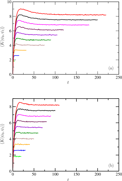
Figure 1: (Color online) The average of $K(\psi_{0},\psi_{t})=-\ln F(\psi_{0},\psi_{t})$ vs. time in the local scheme (a) and in the non-local scheme (b). The number of qubits in the register is $n=2,3,\dots,11$ qubits (from bottom to top).

In Fig. 1 we present $\langle K(\psi_{0},\psi_{t})\rangle$ vs. $t$, averaged over 2000 realizations, for the local scheme [Fig. 1(a)] and for the non-local scheme [Fig. 1(b)]. The sharp increase of $\langle K(\psi_{0},\psi_{t})\rangle$ is explained by the fact that the fidelity is highly sensitive not only to two-qubit operations but also to single-qubit operations. Hence, the first few steps of the scheme can decrease the fidelity substantially. To explain the overshoot, notice that product states have smaller fidelity with each other than entangled states, since the fidelity of two product states is simply the multiplication of the fidelities of the tensor components (all smaller then 1). In the beginning of the scheme, the register is still nearly separable so its fidelity with the (also separable) initial state is smaller than when it is completely entangled. After a sufficient number of steps, the state of the register is uncorrelated with the input state, and $\langle K(\psi_{0},\psi_{t})\rangle$ saturates. As the number of qubits in the register increases, it takes more steps to bring $\langle K(\psi_{0},\psi_{t})\rangle$ to saturation. However, there is no significant difference between the two geometries.

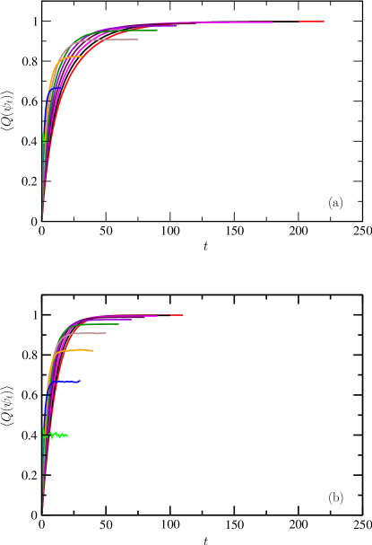
Figure 2: (Color online) The average of the entanglement measure $Q(\psi_{t})$ vs. $t$ in the local scheme (a) and in the non-local scheme (b), for a register with $2,3,\dots,11$ qubits, from bottom to top. Clearly, the entanglement builds up faster in the non-local scheme.

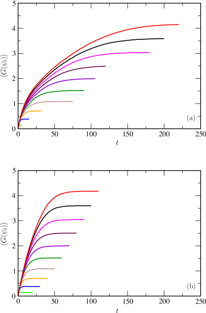
Figure 3: (Color online) The average of the Groverian measure $G(\psi_{t})$ vs. $t$ in the local scheme (a) and in the non-local scheme (b), for a register with $2,3,\dots,11$ qubits. The Groverian measure increases faster in the non-local scheme.

The average bipartite entanglement, $\langle Q(\psi_{t})\rangle$, is shown in Figs. 2(a) for the local scheme and in Fig. 2(b) for the non-local scheme. It increases more slowly than $\langle K(\psi_{0},\psi_{t})\rangle$. The asymptotic value of $\langle Q(\psi_{t})\rangle$ is the same for both geometries, but it is reached much faster in the non-local geometry than in the local, one dimensional geometry. The results for the one dimensional geometry are consistent with those presented in Ref. Emerson2003 . The Groverian measure $G(\psi_{t})$ vs. $t$ is shown in Fig. 3(a) and 3(b), for the local and non-local geometries, respectively. Clearly, $\langle G(\psi_{t})\rangle$ converges to its asymptotic value more slowly than $\langle Q(\psi)\rangle$. The asymptotic value of $\langle G(\psi)\rangle$ is the same for both geometries but it is reached much faster in the non-local geometry.

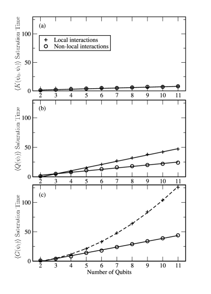
Figure 4: The number of steps required for the averages of $K(\psi_{0},\psi_{t})$ (a), $Q(\psi_{t})$ (b) and $G(\psi_{t})$ (c) to reach 90% of their saturation values in the local ($+$) and in the non-local ($\circ$) schemes vs. the number of qubits in the register. While the results for $K(\psi_{0},\psi_{t})$ are nearly identical in both schemes, the time required for $Q(\psi_{t})$ and $G(\psi_{t})$ to converge is shorter in the non-local scheme. The solid lines are linear fits and the dashed line is a quadratic fit.

The number of steps required for $\langle K(\psi_{0},\psi_{t})\rangle$, $\langle Q(\psi_{t})\rangle$, and $\langle G(\psi_{t})\rangle$, to reach 90% of their saturation values, vs. $n$, is shown in Figs. 4(a), 4(b) and 4(c), respectively. The results for $\langle K(\psi_{0},\psi_{t})\rangle$ are almost identical in the local and non-local schemes. The time it takes $\langle Q(\psi_{t})\rangle$, to reach 90% of its saturation values appears to be linear in $n$, for both geometries. However, the slope is lower for the non-local geometry, which means that the average bipartite entanglement builds up more quickly when non-local interactions are allowed. Similarly, in the non-local geometry the saturation time of $\langle G(\psi)\rangle$ is linear in $n$. In the local geometry, the saturation time is longer and it deviates from linear dependence on $n$ and is well fitted by a quadratic function of $n$.

In the analysis above we focused on the averages of functions $K$, $Q$ and $G$. Each data point was obtained by averaging over at least 2000 runs of the entanglement forming procedure described above. These averages were taken from the distributions $f(K)$, $f(Q)$ and $f(G)$ for the quantum states $|\psi_{t}\rangle$ obtained after $t$ iterations of the procedure. As $t$ increases, these distributions are found to approach the distribution obtained for random states of the register Emerson2003 . In Fig. 5 we present the probability densities $f(G)$ of the Groverian measure $G(\psi_{t})$, for $t=10$ (dashed-dotted line), $20$ (dashed line) and $100$ (solid line) steps, for a register with $n=8$ qubits. As the number of steps increases, these distributions approach the distribution $f(G)$ obtained for pseudo-random states of the 8-qubit register (dotted line).

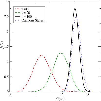
Figure 5: (Color online) The probability density $f(G)$ of the Groverian measure $G(\psi_{t})$ for the states obtained after $t=10$ (dashed-dotted line), 20 (dahsed line) and 100 (solid line) iterations of the entanglement forming procedure, for $n=8$ qubits. As $t$ increases, the distribution converges to the one obtained for pseudo-random states (dotted line).

These results indicate that building up bipartite as well as multipartite entanglement, using two-qubit gates is more efficient when non-local interactions are allowed. Furthermore, in both geometries it seems that multipartite entanglement, evaluated by $G(\psi)$ builds up more slowly than the bipartite-like entanglement, quantified by $Q(\psi)$.

V Discussion

Quantum algorithms are typically designed under the assumption that two-qubit operations are possible between any pair of qubits. However, some of the physical realizations of quantum computation allow only local interactions between neighboring qubits DiVincenzo2000 . In these realizations, non-local operations are achieved using swap gates Aharonov1997 , which may involve a significant overhead Schuch2003 . To put the results of this paper in the context of known physical realizations, we briefly review below several such realizations and specify whether they are based on local or non-local interactions.

Ion-trap quantum computing devices Cirac1995 ; Kielpinski2003 consist of laser-cooled ions, which are electromagnetically confined in ultra-high vacuum. The spin states of the ions are used as qubits. Single-qubit gates are preformed by selectively applying electromagnetic fields on the different ions. Two-qubit gates are realized through a global phonon state, which makes use of the collective vibrational degree of freedom of the ions. The ground state and the first excited state of the phonon comprise a two-level system, which is used as an additional qubit. Using carefully tuned laser-induced transitions, two-qubit gates can be applied between each ion and the global phonon. Specifically, a swap gate can be applied between them, enabling to apply two-qubit gates between any pair of qubits. Ion traps thus provide a non-local implementation of quantum computation. Linear optics provides another non-local realization of quantum computation Knill2001 ; Kok2007 .

Quantum computation can also be performed using solid state devices Cerletti2005 ; Burkard2004 . Several proposals are comprised of qubits based on superconducting Josephson junctions Makhlin2001 . One such proposal uses the two states of a superconducting single-charge box as a charge-qubit. The possibility of connecting all the qubits in parallel to a common LC-oscillator mode was suggested as a way to apply two-qubit gates Makhlin1999 . This parallel connection, together with the ability to simultaneously control the Josephson coupling for each qubit, allows two-qubit interaction between any pair of qubits, giving rise to a non-local scheme. A different superconducting scheme is based on Josephson flux qubits, which interact through magnetic induction. Unlike the charge-qubit scheme, the flux-qubit scheme is a local one. Another implementation is based on electron spins as qubits, confined to quantum dots Loss1998 . Two-qubit gates are applied using a time-dependent Heisenberg exchange coupling between adjacent dots, providing a local scheme for quantum computation. Solid state realizations may be most suitable for scalable implementation of quantum computations. Some of these realizations are based on local interactions. Local interactions appear form multiple-qubit entanglement at a lower rate than non-local interactions. However, the connection between the entanglement as quantified by the Groverian and related measures and the speedup offered by quantum algorithms is not yet clear.

VI Summary

We have studied the formation of multipartite quantum entanglement by repeated operation of one and two qubit gates. The resulting entanglement was evaluated using the average bipartite and the Groverian measures. A comparison was made between two geometries of the quantum register: a non-local geometry in which any pair of qubits may interact and a local geometry in which the qubits are arranged in a one dimensional chain, where only nearest neighbor interactions are allowed. More specifically, we used a combination of random single qubit rotations and a fixed two-qubit operation, namely the controlled phase gate. We found that in this scheme, entanglement is generated more quickly in the non-local geometry than in the one-dimensional chain. Thus, non-local implementations of quantum computation are expected to be more efficient in generating highly entangled states.

References

- (1) P.W. Shor, in Proceedings of the 35th Annual Symposium on the Foundations of Computer Science, edited by S. Goldwasser (IEEE Computer Society, Los Alamitos, CA, 1994), p. 124.
- (2) L. Grover, in Proceedings of the Twenty-Eighth Annual Symposium on the Theory of Computing (ACM Press, New York, 1996), p. 212.
- (3) L.K. Grover, Phys. Rev. Lett. 79, 325 (1997).
- (4) R. Jozsa and N. Linden, Proc. R. Soc. London, Ser. A 459, 2011 (2003).
- (5) G. Vidal, Phys. Rev. Lett. 91, 147902 (2003).
- (6) D. Aharonov and M. Ben-Or, in Proceedings of the 37th Annual Symposium on the Foundations of Computer Science, edited by S. Goldwasser (IEEE Computer Society, Los Alamitos, CA, 1996), p. 46.
- (7) C. H. Bennett, H. J. Bernstein, S. Popescu, and B. Schumacher, Phys. Rev. A 53, 2046 (1996).
- (8) C.H. Bennett, D.P DiVincenzo, J.A.Smolin and W.K Wootters, Phys. Rev. A 54, 3824 (1996).
- (9) S. Hill and W.K. Wootters, Phys. Rev. Lett. 78, 5022 (1997).
- (10) W.K. Wootters, Phys. Rev. Lett. 80, 2245 (1998).
- (11) V. Vedral, M.B. Plenio, M.A. Rippin and P.L. Knight, Phys. Rev. Lett. 78, 2275 (1997).
- (12) V. Vedral and M.B. Plenio, Phys. Rev. A 57, 1619 (1998).
- (13) G. Vidal, J. Mod. Optics 47, 355 (2000).
- (14) M. Horodecki, P. Horodecki and R. Horodecki, Phys. Rev. Lett. 84, 2014 (2000).
- (15) V. Vedral, M. B. Plenio, K. Jacobs, and P. L. Knight, Phys. Rev. A 56, 4452 (1997).
- (16) H. Barnum and N. Linden, J. Phys. A 34, 6787 (2001).
- (17) M.S. Leifer, N. Linden and A. Winter, Phys. Rev. A 69, 052304 (2004).
- (18) M. A. Nielsen and I. L. Chuang , Quantum computation and quantum information (Cambridge University Press, Cambridge, 2000).
- (19) A. Barenco, C.H. Bennett, R. Cleve, D.P. DiVincenzo, N. Margolus, P. Shor, T. Sleator, J.A. Smolin and H. Weinfurter, Phys. Rev. A 52, 3457 (1995).
- (20) D.P. DiVincenzo, Fortsch. der Phys. 48, 771 (2000).
- (21) D. Aharonov and M. Ben-Or, Fault-tolerant quantum computation with constant error, Proceedings of the 29th Ann. ACM Symposium on the Theory of Computing (El-Paso, Texas, May 1997), p. 176.
- (22) D. Gottesman, J. Mod. Optics 47, 333 (1999).
- (23) A.G. Fowler, C.D. Hill and L.C.L. Hollenberg, Phys. Rev. A 69, 042314 (2004).
- (24) A.G. Fowler, S.J. Devitt and L.C.L. Hollenberg, Quantum Inform. Comput. 4, 237 (2004).
- (25) M. Möttönen and J.J. Vartiainen, Decompositions of general quantum gates, (arxiv e-print: quant-ph/0504100).
- (26) M.B. Plenio and F.L. Semião, New J. Phys. 7, 73 (2005).
- (27) D.A. Meyer and N.R. Wallach, J. Math. Phys. 43, 4273 (2002).
- (28) G.K. Brennen, Quantum Inform. Comput. 3, 619 (2003).
- (29) J. Emerson, Y.S. Winstein, M. Saraceno, S. Lloyd and D.G. Cory, Science 302, 2098 (2003).
- (30) O. Biham, M.A. Nielsen and T.J. Osborne, Phys. Rev. A 65, 062312 (2002).
- (31) B. Kraus and J.I. Cirac, Phys. Rev. A 63, 062309 (2001).
- (32) Y.S. Weinstein and C.S. Hellberg, Phys. Rev. Lett. 95, 030501 (2005).
- (33) Y. Shimoni and O. Biham, Phys. Rev. A 75, 022308 (2007).
- (34) O. Biham, D. Shapira and Y. Shimoni, Phys. Rev. A 68, 022326 (2003).
- (35) A. Miyake and M. Wadati, Phys. Rev. A 64, 042317 (2001).
- (36) Y. Shimoni, D. Shapira and O. Biham, Phys. Rev. A 69, 062303 (2004).
- (37) Y. Shimoni, D. Shapira and O. Biham, Phys. Rev. A 72, 062308 (2005).
- (38) D. Shapira, Y. Shimoni and O. Biham, Phys. Rev. A 73, 044301 (2006).
- (39) R. Oliveira, O.C.O. Dahlsten and M.B. Plenio, Phys. Rev. Lett. 98, 130502 (2007).
- (40) K. Życzkowski and M. Kuś, J. Phys. A 27, 4235 (1994).
- (41) N. Schuch and J. Siewert, Phys. Rev. A 67, 032301 (2003).
- (42) J.I. Cirac and P. Zoller, Phys. Rev. Lett. 74, 4091 (1995).
- (43) D. Kielpinski, J. Opt. B 5, 121 (2003).
- (44) E. Knill, R. Laflamme and G.J. Milburn, Nature 409, 46 (2001).
- (45) P. Kok, W.J. Munro, K. Nemoto, J.P. Dowling and G.J. Milburn, Rev. Mod. Phys. 79, 135 (2007).
- (46) V. Cerletti, W.A. Coish, O. Gywat and D. Loss, Nanotechnology 16, 27 (2005).
- (47) G. Burkard, Theory of solid state quantum information processing, (arxiv e-print: cond-mat/0409626).
- (48) Y. Makhlin, G. Schön and A. Shnirman, Rev. Mod. Phys. 73, 357 (2001).
- (49) Y. Makhlin, G. Schön and A. Shnirman, Nature 386, 305 (1999).
- (50) D. Loss and D.P. DiVincenzo, Phys. Rev. A 57, 120 (1998).