Disordered Correlated Kondo-lattice model

Abstract

We propose a self-consistent approximate solution of the disordered Kondo-lattice model (KLM) to get the interconnected electronic and magnetic properties of ’local-moment’ systems like diluted ferromagnetic semiconductors. Aiming at $(A_{1-x}M_{x})$ compounds, where magnetic (M) and non-magnetic (A) atoms distributed randomly over a crystal lattice, we present a theory which treats the subsystems of itinerant charge carriers and localized magnetic moments in a homologous manner. The coupling between the localized moments due to the itinerant electrons (holes) is treated by a modified RKKY-theory which maps the KLM onto an effective Heisenberg model. The exchange integrals turn out to be functionals of the electronic selfenergy guaranteeing selfconsistency of our theory. The disordered electronic and magnetic moment systems are both treated by CPA-type methods.

We discuss in detail the dependencies of the key-terms such as the long range and oscillating effectice exchange integrals, ’the local-moment’ magnetization, the electron spin polarization, the Curie temperature as well as the electronic and magnonic quasiparticle densities of states on the concentration $x$ of magnetic ions, the carrier concentration $n$, the exchange coupling $J$, and the temperature. The shape and the effective range of the exchange integrals turn out to be strongly $x$-dependent. The disorder causes anomalies in the spin spectrum especially in the low-dilution regime, which are not observed in the mean field approximation.

I Introduction

There are many analytical models such as the Hubbard and the Anderson models which are very useful for the description of real correlated electron systems. The Kondo-lattice Model (KLM) is yet another one. The KLM describes an interplay of itinerant electrons in a partially filled energy band with magnetic moments localized at certain lattice sites Nolting0 ; Edw ; Furukawa . The characteristic model properties result from an interband exchange interaction between two well-defined subsystems: itinerant electrons and localized spins. This model has a long history, particularly concerning with itinerant electron magnetism Moriya , heavy fermion systems Stewart , perovskite manganese oxides Furukawa , and so on.

Problems connected with the substitutional disorder have recently become more and more important in different fields of material science, e.g., the diluted magnetic semiconductors (DMS) MacDonald , the transition metal dielectrics Gusev , etc. Extensive theoretical work on the problem of disorder has been done for random Heisenberg spin systems Harris ; DveyAharon ; Theumann ; Theumann01 ; TahirKheli ; Gurskii ; Sherrington ; Sherrington01 ; Fibich .

Here, we are mainly interested on how the disorder influences the characteristic properties of local-moment systems such as the DMS, where magnetic ($M$) and non-magnetic ($A$) atoms are distributed randomly over a crystal lattice ($A_{1-x}M_{x}$) with a given concentration of magnetic atoms $x$. In order to answer this question different approaches were proposed Theumann ; Harris ; Jones ; Kudrnovsky ; Fibich ; Bouzerar01 . More or less realistic electronic structure calculations based on density functional theory (DFT) or numerical methods like classical Quantum Monte Carlo were used for standard models like the Heisenberg spin system Hilbert . However, the disadvantage of the realistic DFT-calculations come from their strong material dependence Kudrnovsky . Therefore, they do not explain the basic physics of disordered local-moment systems in a simple way. But, it is known that a disordered KLM Hamiltonian can be mapped onto an random Heisenberg model(shown in the text), so, in this respect better results can be obtained from its model study.

A special challenge when treating the random Kondo-lattice model arises with the fact that both the electron and the spin subsystem have to be considered simultaneously and on the same level. Most of the KLM investigations are focused on the electronic Takahashi ; Blackman01 or magnetic Theumann ; Harris ; Fibich ; Bouzerar2 ; Hilbert ; Bouzerar01 subsystem only. A special goal of our study is the homologous treatment of the electronic and magnetic properties of the random KLM, which mutually effect each other and, therefore, should be determined self-consistently.

Nevertheless, we are forced to apply different methods to study the influence of the disorder and dilution of the magnetic moments subsystem on the properties of these two aforementioned subsystems. In this paper for the itinerant electron system a proper alloy analogy with the respective coherent potential approximation (CPA) Elliott is used. For the random spin system, for which the situation is not so clear, an equivalent ansatz must be found. As it was done successfully for the periodic KLM Nolting0 (’modified’ RKKY (MRKKY)) one can map the KLM-interband exchange on an effective and random Heisenberg model. The resulting effective exchange integrals between the localized spins will be long range and complicated functionals of the electronic self-energy. The conventional RKKY, resulting from second order perturbation theory is insufficient even with a phenomenological damping factor Kudrnovsky ; Bouzerar2 . Higher order conduction electron self-energy effects, being taken into account by ’modified’ RKKY but neglected by conventional $RKKY$, provide the self-consistency of the full KLM. They drastically influence the magnetic properties such as the Curie temperature.

A similar strategy of treating the disordered Kondo-lattice model has recently been used in ref. Tang , namely the combination of partial solutions for the electronic and magnetic part by a modified RKKY theory. However, the authors use different methods in order to solve the partial problems. For the electronic part, they apply a procedure which gives correct results only for very low band occupation. For the spin part, on the other hand, the disorder has been solved by a mean-field ansatz. In this paper we present alternative treatments of these partial problems. In particular, we develop a better technique to deal with the spin disorder. The band electrons are discussed within CPA starting from an atomic limit alloy analogy without any restriction to the electron band occupation. Several anomalies in the spin spectrum are found, which are not reproducible by the method of ref. Tang .

The paper is organized as follows: In Sec. 2 we describe the methods and approximations that we have chosen to study electron and spin dynamics in the disordered KLM. Numerical results concerning Curie temperatures, the magnon densities of states and the effective exchange integrals are presented in Sec. 3 for wide range of the model parameters like exchange coupling $J$, concentration of magnetic atoms $x$, electron band occupation $n$, and temperature $T$. Section 4 is assigned for a summary and an outlook.

II Theoretical Model

The correlated KLM-Hamiltonian can be written in second quantized form as the sum of a kinetic energy, an exchange interaction, and a Hubbard-type Coulomb interaction

$$\hat{H}^{K}=\sum_{i,j,\sigma}t_{ij}a^{+}_{i\sigma}a_{j\sigma}+\frac{U}{2}\sum_{i\sigma}n_{i\sigma}n_{i,-\sigma}-\frac{J}{2}\sum_{i\sigma}\left\{z_{\sigma}S^{z}_{i}a^{+}_{i\sigma}a_{i\sigma}+S^{\sigma}_{i}a^{+}_{i,-\sigma}a_{i\sigma}\right\},$$ (1)

where;

$$z_{\sigma}=\delta_{\sigma\uparrow}-\delta_{\sigma\downarrow},S^{\sigma}_{i}=S^{x}_{i}+iz_{\sigma}S^{y}_{i},$$ (2)

and $a^{+}_{i\sigma}\left(a_{i\sigma}\right)$ is the creation (annihilation) operator for the Wannier electron with the spin $\sigma\left(\sigma=\uparrow,\downarrow\right)$ at the site $\vec{R}_{i}$, $J$ is an exchange coupling which we assume to be positive in the following theory, $t_{ij}$ is an electron hopping integral between lattice sites, $U$ is the Coulomb interaction, and $N$ is the total number of crystal sites. The inclusion of the Hubbard-term to the standard-KLM has only the reason to push doubly occupied levels above the Fermi level. This will be further commented on in section 2.1 where we discuss the electronic subsystem.

In order to introduce the disorder into KLM of the $A_{1-x}M_{x}$ type, we introduce projection operators;

$$X^{A}_{i}=\begin{cases}1,&\text{{- if site $i$ is $A$}}\\ 0,&\text{{- otherwise,}}\end{cases}$$ (3)

$$X^{M}_{i}=\begin{cases}1,&\text{{- if site $i$ is $M$}}\\ 0,&\text{{- otherwise.}}\end{cases}$$ (4)

Using these definitions we can change the notations in the Hamiltonian (1) for the disorder in hopping and exchange coupling terms, respectively;

$$\begin{array}[]{c}t_{ij}\rightarrow\sum_{k,\acute{k}\in A,M}t^{k\acute{k}}X^{k}_{i}X^{\acute{k}}_{j},\\ J\rightarrow\sum_{k\in A,M}J^{k}X^{k}_{i},\end{array}$$ (5)

where hopping parameters $t^{AA}=t^{MM}=t^{AM}=t^{MA}=t=W/6$ are the same for the different kind of atoms and are equivalent to a half band width $W$ for the case of a simple cubic lattice, and exchange couplings are $J^{M}=J,J^{A}=0$ for magnetic and nonmagnetic atoms, respectively.

After configurational averaging these operators are simply expressed by the concentration $x$ of magnetic atoms $M$.

$$\begin{array}[]{l}\left\langle X^{A}_{i}\right\rangle_{c}=1-x,\\ \left\langle X^{M}_{i}\right\rangle_{c}=x.\end{array}$$ (6)

In order to study conduction-electron properties, we use the configurationally averaged single-electron Green function;

$$G_{ij\sigma}\left(E\right)=\overline{\left\langle\left\langle a_{i\sigma}|a^{+}_{j\sigma}\right\rangle\right\rangle_{E}}.$$ (7)

Where the symbol $\overline{(\ldots})$ denotes the configurational ensemble average.

The relation between the band occupation $n$ and the chemical potential $\mu$ is as follows:

$$n=n_{\uparrow}+n_{\downarrow}=-\frac{1}{\pi}\sum_{\sigma}\int^{\infty}_{-\infty}\frac{ImG_{ii,\sigma}(E)}{e^{\beta(E-\mu)}+1}dE,$$ (8)

with $\beta=1/kT$ is the inverse temperature.

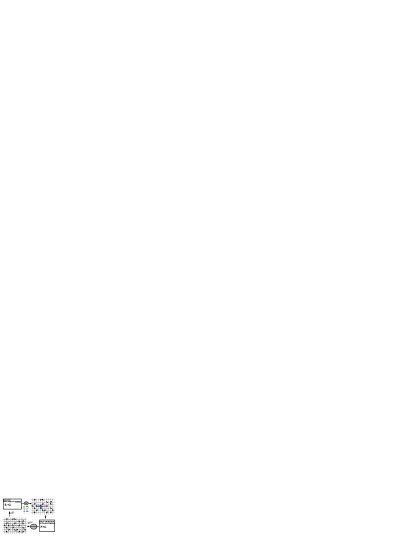
Figure 1: General procedure of the self-consistent mapping of the disordered Kondo-lattice model onto disordered Heisenberg model

The main idea of this paper is to map the disordered KLM on an effective random isotropic spin Heisenberg Hamiltonian;

$$\hat{H}^{RH}=-\frac{1}{2}\sum_{ij}J_{ij}X^{M}_{i}X^{M}_{j}\left(S^{z}_{i}S^{z}_{j}+S^{+}_{i}S^{-}_{j}\right),$$ (9)

where $J_{ij}$ is an effective exchange interaction between localized magnetic moments. We assume that we can calculate the effective exchange interaction, $J_{ij}$, using the MRKKY method Nolting0 ; Nolting1 ; Nolting2

$$J_{\vec{q}}=\frac{J^{2}}{4\pi}\int^{\infty}_{-\infty}\frac{dE}{e^{\beta(E-\mu)}+1}\frac{1}{N}\sum_{\sigma,\vec{k}}Im\left[G^{0}_{\vec{k}}\left(E\right)G_{\vec{k}+\vec{q},\sigma}\left(E\right)\right],$$ (10)

which in the weak-coupling limit agrees with conventional RKKY, where $J_{\vec{q}}$ is the Fourier-transform of $J_{ij}$. Then we get the full self-consistent loop for a finite temperature calculation (see Fig. 1). In order to study magnetic properties of the disordered KLM we calculate the configurationally averaged magnon Green function:

$$D_{\vec{q}}\left(E\right)=\overline{\left\langle\left\langle S^{+}_{\vec{q}}|S^{-}_{-\vec{q}}\right\rangle\right\rangle_{E}}.$$ (11)

Using Callen equation Callen , it is then possible to calculate the magnetization $\left\langle S^{z}\right\rangle$:

$$\left\langle S^{z}\right\rangle=\frac{\left(S-\phi\right)\left(1+\phi\right)^{2S+1}+\left(S+1+\phi\right)\phi^{2S+1}}{\left(1+\phi\right)^{2S+1}-\phi^{2S+1}},$$ (12)

where

$$\phi=-\frac{1}{\pi}\frac{1}{N}\sum_{\vec{q}}\int^{\infty}_{0}\frac{ImD_{\vec{q}}\left(E\right)}{e^{\beta E}-1}dE.$$ (13)

The procedure presented in Fig. 1 is very general. It is clear that we have to use different approximations in order to solve the disordered electronic and magnetic parts. Now, we discuss these approximations in more detail.

II.1 Electron Subsystem: Zero-bandwidth limit of the correlated KLM

The total Hamiltonian of the correlated KLM model is given by (1).

The zero-bandwidth limit Nolting2 is defined by

$$t_{ij}\rightarrow 0.$$ (14)

In this approximation the excitation spectrum consists of the following four poles Nolting2

$$\begin{array}[]{ll}\epsilon_{1}=-\frac{1}{2}JS,&\epsilon_{2}=\frac{1}{2}J\left(S+1\right),\\ \epsilon_{3}=U+\frac{1}{2}JS,&\epsilon_{4}=U-\frac{1}{2}J\left(S+1\right).\end{array}$$ (15)

It means that the single electron spectral density $A_{\sigma}\left(E\right)$ must be a four-pole function

$$A_{\sigma}\left(E\right)=\sum_{m=1}^{4}\alpha_{m\sigma}\delta\left(E-\epsilon_{m}\right).$$ (16)

The temperature- and concentration-dependent coefficients $\alpha_{m\sigma}$ have the physical meaning of spectral weights for the corresponding excitation energies. The expressions for these weight-factors are Nolting2 :

$$\begin{array}[]{l}\alpha_{1\sigma}=\frac{1}{2S+1}\left(S+1+z_{\sigma}\left\langle S^{z}\right\rangle-\left(S+1\right)n_{-\sigma}+\Delta_{-\sigma}\right),\\ \alpha_{2\sigma}=\frac{1}{2S+1}\left(S-z_{\sigma}\left\langle S^{z}\right\rangle-Sn_{-\sigma}-\Delta_{-\sigma}\right),\\ \alpha_{3\sigma}=\frac{1}{2S+1}\left(\left(S+1\right)n_{-\sigma}+\Delta_{-\sigma}\right),\\ \alpha_{4\sigma}=\frac{1}{2S+1}\left(Sn_{-\sigma}-\Delta_{-\sigma}\right),\end{array}$$ (17)

where $\Delta_{\sigma}=\left\langle S^{\sigma}a_{-\sigma}^{+}a_{\sigma}\right\rangle+z_{\sigma}\left\langle S^{z}n_{\sigma}\right\rangle$ is a mixed spin-electron correlation function.

The term $\Delta_{\sigma}$ can be expressed by the single-electron Green function Nolting1 :

$$\Delta_{\sigma}=-\frac{1}{\pi J}\frac{1}{N}\sum_{\vec{k}}\int^{\infty}_{-\infty}\frac{dE}{e^{\beta\left(E-\mu\right)}+1}\left(E-t_{\vec{k}}\right)ImG_{\vec{k}\sigma}\left(E\right).$$ (18)

A propagating $\sigma$ electron will meet at a certain lattice site $\vec{R_{i}}$ the atomic level $\epsilon_{1}$ with probability $\alpha_{1\sigma}$, the level $\epsilon_{2}$ with probability $\alpha_{2\sigma}$ and so on, if there is no correlation between sites. This leads to the four-component alloy. Eq. (15) makes clear that without the Coulomb interaction $U$ the pole $\epsilon_{4}$ would be the lowest energy. According to the spectral weight $\alpha_{4\sigma}$ in eq. (17), however, $\epsilon_{4}$ requires a double occupancy of the lattice site. $\epsilon_{4}$ to be the lowest energy therefore appears unphysical.On the other hand, for strong enough U it will not play any role.

It is easy to generalize this alloy analogy to a disordered KLM. We have to take into consideration the non-magnetic sites $\epsilon_{5}=\epsilon_{A}$ as the fifth alloy constituent with the spectral weight $1-x$. The excitation spectrum is then:

$$\begin{array}[]{lll}\epsilon_{m}&\rightarrow&\tilde{\alpha}_{m\sigma}=x\alpha_{m\sigma},\\ \epsilon_{5}=0&\rightarrow&\tilde{\alpha}_{5\sigma}=1-x.\end{array}$$ (19)

This zero-bandwidth alloy analogy is the basic framework for applying CPA to get the electronic selfenergy.

$$\Sigma_{\sigma}(E)=\sum_{m=1}^{5}\tilde{\alpha}_{m\sigma}\frac{\epsilon_{m}}{1-(\epsilon_{m}-\Sigma_{\sigma}(E))G_{0}(E-\Sigma_{\sigma}(E))},$$ (20)

where

$$G_{0}(E)=\frac{1}{N}\sum_{\vec{k}}\frac{1}{E-t_{\vec{k}}}.$$ (21)

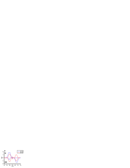
Figure 2: Density of electron states for the disordered KLM at a)$x=0.95$;b)$x=0.1,U\rightarrow\infty,W=0.5eV,n=0.06,S=5/2,J=0.4eV$ for ferromagnetic $\left\langle S^{z}\right\rangle=S$ and paramagnetic $\left\langle S^{z}\right\rangle=0$ cases

Therewith we can write the electron Green function:

$$G_{\vec{k},\sigma}(E)=\frac{1}{E-\Sigma_{\sigma}(E)-t_{\vec{k}}},$$ (22)

where $t_{\vec{k}}$ is the Fourier transform of the hopping integral $t_{ij}$. The quasiparticle density of states (DOS) is derived essentially from imaginary part of the Green function:

$$\rho_{\sigma}(E)=-\frac{1}{\pi N}\sum_{\vec{k}}\textit{Im}G_{\vec{k},\sigma}(E).$$ (23)

Fig. 2 represents the quasiparticle density of states for large and small concentrations x of M atoms in full saturation $\left\langle S^{z}\right\rangle=S$ and paramagnetic $\left\langle S^{z}\right\rangle=0$ limits, respectively. In the case of strong Coulomb interaction($U\rightarrow\infty$), the DOS consists in general of three subbands. For $\left\langle S^{z}\right\rangle=S(T=0)$ the spin up electron density is absent for energies around $J(S+1)/2$, while the spin down density is finite there.

In the limit $x=0$, our model reduces to the well-known Hubbard model. It has been shown Vollhardt that in infinite lattice dimension the CPA is an exact treatment of the alloy problem. But, the question, however, is: what is the optimal alloy analogy for the Hubbard model? The conventional atomic-limit starting point, which we have applied, may be questionable for the pure Hubbard model. It is known (Ref. Schneider ) that this alloy analogy does not allow for describing band-ferromagnetism. But, since we are interested only in the ferromagnetism due to the interband exchange $J$, we believe that the alloy analogy (Eq. 14-18) is appropriate for the correlated Kondo-lattice model although the Hubbard limit can be improved, for e.g. by the modified alloy analogy Potthoff .

II.2 Spin Subsystem

Let us now consider a structurally disordered system of $N_{M}=xN$ spins which can be described by the isotropic Heisenberg Hamiltonian

$$\hat{H}=-\sum_{ij}J_{ij}X^{M}_{i}X^{M}_{j}\left(S^{z}_{i}S^{z}_{j}+S^{+}_{i}S^{-}_{j}\right).$$ (24)

We use two-time temperature Green functions for the investigation of spin excitations. The Green function within Tyablikov approximation satisfies the equation of motion

$$\begin{array}[]{l}E\left\langle\left\langle S_{l}^{+}|S_{k}^{-}\right\rangle\right\rangle_{E}=2\delta_{lk}X^{M}_{l}\left\langle S^{z}_{l}\right\rangle+\\ 2\sum_{j\neq l}J_{lj}\left\langle\left\langle X^{M}_{j}\left\langle S^{z}_{j}\right\rangle S_{l}^{+}-\left\langle S^{z}_{l}\right\rangle X^{M}_{l}S_{j}^{+}|S_{k}^{-}\right\rangle\right\rangle_{E}.\end{array}$$ (25)

After Fourier transformation to wave vectors, the above equation of motion can be written as:

$$\begin{array}[]{l}\left(E-x\left\langle S^{z}\right\rangle E_{0}(\vec{q})\right)\left\langle\left\langle S_{\vec{q}}^{+}|S_{\vec{q^{\prime}}}^{-}\right\rangle\right\rangle_{E}=\\ 2x\left\langle S^{z}\right\rangle\delta(\vec{q}+\vec{q^{\prime}})+2\left\langle S^{z}\right\rangle\frac{1}{\sqrt{N}}\Delta X_{\vec{q}+\vec{q^{\prime}}}+\\ 2\left\langle S^{z}\right\rangle\sum_{\vec{k}}\left(J(\vec{q}-\vec{k})-J(\vec{k})\right)\frac{1}{\sqrt{N}}\Delta X_{\vec{q}+\vec{k}}\left\langle\left\langle S_{\vec{k}}^{+}|S_{\vec{q^{\prime}}}^{-}\right\rangle\right\rangle_{E},\end{array}$$ (26)

where we have used

$$\begin{array}[]{c}\Delta X_{\vec{q}}=X_{\vec{q}}-x\sqrt{N}\delta({\vec{q}}),\\ X_{\vec{q}}=\frac{1}{\sqrt{N}}\sum_{i=1}^{N}X^{M}_{i}e^{-i\vec{q}\vec{R_{i}}}\\ E_{0}(\vec{q})=2x\left\langle S^{z}\right\rangle(J(0)-J(\vec{q}))\end{array}$$ (27)

The approximation $\left\langle S^{z}\right\rangle=\overline{\left\langle S^{z}_{l}\right\rangle}$ is very often applied to disordered systems and means the neglect of structural fluctuations of spin positions.

Averaging over all possible realizations of atomic configurations, the equation for averaged Green function can be written in the following form:

$$\begin{array}[]{l}\left(E-E_{0}(\vec{q})\right)\overline{\left\langle\left\langle S_{\vec{q}}^{+}|S_{\vec{q^{\prime}}}^{-}\right\rangle\right\rangle}_{E}=2x\left\langle S^{z}\right\rangle\delta(\vec{q}+\vec{q^{\prime}})+\\ 2\left\langle S^{z}\right\rangle\sum_{\vec{k}}\left(J(\vec{q}-\vec{k})-J(\vec{k})\right)\frac{1}{\sqrt{N}}\overline{\Delta X_{\vec{q}+\vec{k}}\left\langle\left\langle S_{\vec{k}}^{+}|S_{\vec{q^{\prime}}}^{-}\right\rangle\right\rangle}_{E}.\end{array}$$ (28)

The equation contains a higher-order averaged Green function $\overline{\Delta XG}$. One can write the equation of motion for this function, multiplying it by $\Delta X$ and performing configurational average which will include terms like, $\overline{\Delta X\Delta XG}$. In order to solve these equations, the following decoupling of configurational averages is used;

$$\overline{\Delta X_{\vec{q}-\vec{k}}\Delta X_{\vec{k}-\vec{k^{\prime}}}\left\langle\left\langle S_{\vec{k^{\prime}}}^{+}|S_{\vec{q^{\prime}}}^{-}\right\rangle\right\rangle}\approx\overline{\Delta X_{\vec{q}-\vec{k}}\Delta X_{\vec{k}-\vec{k^{\prime}}}}\overline{\left\langle\left\langle S_{\vec{k^{\prime}}}^{+}|S_{\vec{q^{\prime}}}^{-}\right\rangle\right\rangle},$$ (29)

where

$$\overline{\Delta X_{\vec{q}-\vec{k}}\Delta X_{\vec{k}-\vec{k^{\prime}}}}=\delta(\vec{q}-\vec{k^{\prime}})\overline{\Delta X_{\vec{q}-\vec{k}}\Delta X_{\vec{k}-\vec{q}}}.$$ (30)

The equation exploits translation symmetry.

Thus, for the averaged Green function, we eventually get;

$$\begin{array}[]{l}\overline{\left\langle\left\langle S_{\vec{q}}^{+}|S_{\vec{q^{\prime}}}^{-}\right\rangle\right\rangle_{E}}=\delta(\vec{q}+\vec{q^{\prime}})\frac{2x\left\langle S^{z}\right\rangle+P(\vec{q};E)}{E-E_{0}(\vec{q})-\Sigma(\vec{q};E)},\\ P(\vec{q};E)=\frac{1}{N}\sum_{\vec{k}}\frac{J(\vec{q}-\vec{k})-J(\vec{k})}{E-E_{0}(\vec{k})}S(\vec{q}-\vec{k}),\\ \Sigma(\vec{q};E)=\frac{1}{N}\sum_{\vec{k}}\frac{(J(\vec{q}-\vec{k})-J(\vec{q}))(J(\vec{q}-\vec{k})-J(\vec{k}))}{E-E_{0}(\vec{k})}S(\vec{q}-\vec{k}),\end{array}$$ (31)

where we have introduced the structure factor for the random distribution of magnetic atoms $S(\vec{q})=[\left\langle S^{z}\right\rangle]^{2}\overline{\Delta X_{\vec{q}}\Delta X_{-\vec{q}}}$.

II.2.1 Virtual Crystal Approach

This is the simplest approximation for the magnon Green function. If we neglect all scattering processes $(P=0,\Sigma=0)$ in Eq. (31) we obtain the following expression for the magnon Green function:

$$\overline{\left\langle\left\langle S_{\vec{q}}^{+}|S_{\vec{q^{\prime}}}^{-}\right\rangle\right\rangle_{E}}=\delta(\vec{q}+\vec{q^{\prime}})\frac{2x\left\langle S^{z}\right\rangle}{E-E_{0}(\vec{q})}.$$ (32)

II.2.2 Low Quadratic Approximation

The next simple approach for the structure factor $S(\vec{k})$, while including some scattering processes $(P\neq 0,\Sigma\neq 0)$, is obtained using a cumulant method EdwardsCC ; Matsubara . Using the definition (27) of $X_{\vec{k}}$ variables

$$\overline{\Delta X_{\vec{k}}\Delta X_{-\vec{k}}}=\frac{1}{N}\sum_{i,j}e^{\vec{k}(\vec{R_{i}}-\vec{R_{j}})}(\overline{X^{M}_{i}X^{M}_{j}}-x^{2}),$$ (33)

and the cumulant formula for finding the average of the product of $X^{M}_{i}$ variables EdwardsCC ; Matsubara .

$$\overline{X^{M}_{i}X^{M}_{j}}=\delta_{ij}P_{2}(x)+[P_{1}(x)]^{2}.$$ (34)

where $P_{2}(x)=x(1-x),P_{1}(x)=x$ are second and first cumulants, respectively. Finally, using the following approximation for the structure factor $S(\vec{k})$,

$$S(\vec{k})\rightarrow S^{eff}=[\left\langle S^{z}\right\rangle]^{2}(1-x)x,$$ (35)

we get the expression for the magnon Green function in the Low Quadratic Approximation(LQA) [Ref. Fibich ].

$$\begin{array}[]{l}\overline{\left\langle\left\langle S_{\vec{q}}^{+}|S_{\vec{q^{\prime}}}^{-}\right\rangle\right\rangle_{E}}=\delta(\vec{q}+\vec{q^{\prime}})\frac{2x\left\langle S^{z}\right\rangle+S^{eff}\frac{1}{N}\sum_{\vec{k}}P(\vec{k};E)}{E-E_{0}(\vec{q})-S^{eff}\frac{1}{N}\sum_{\vec{k}}Q(\vec{k};E)},\\ P(\vec{k};E)=\frac{J(\vec{k}-\vec{q})-J(\vec{k})}{E-E_{0}(\vec{k})}\\ Q(\vec{k};E)=\frac{(J(\vec{k}-\vec{q})-J(\vec{k}))(J(\vec{k}-\vec{q})-J(\vec{q}))}{E-E_{0}(\vec{k})}.\end{array}$$ (36)

III Results

Let us discuss some of the results obtained for finite temperature using the self-consistent calculation according to the procedure as sketched in Fig. 1.

Fig. 3 represents the distance-dependence of the effective (MRKKY) exchange integrals for different values of the interband exchange parameter $J$ of the Kondo-lattice model. For the concentrated case ($x=1$) and in the low coupling regime $J\rightarrow 0$ the MRKKY interaction agrees with the conventional RKKY Nolting0 ; Nolting3 . In this situation the effective exchange constant has a long-range character with strong oscillations in the real space. However, with increasing $J$ the MRKKY interaction looses the long range character and transforms into a fairly short-range interaction (like double exchange), where only the first few effective exchange parameters Nolting3 turn out to be important. We realize the same behavior for diluted systems $x<1$. For better comparison with the conventional RKKY, Fig. 3 shows only the oscillation part of the MRKKY interaction $J^{eff}/J^{2}$.

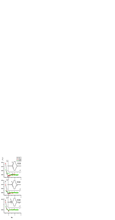
Figure 3: Dependence of the MRKKY interaction (Eq. 10) on the distance $R$ between magnetic atoms in a simple cubic lattice ($R=1$ is a first shell(nearest-neighbors atoms),$R=\sqrt{2}$ is a second shell(next nearest-neighbors atoms) and so on) at fixed parameters $U\rightarrow\infty,W=0.9eV,S=5/2,x=0.1,T=0,\left\langle S^{z}\right\rangle=S$ of the model for three different coupling $J=0.2eV,J=0.4eV,J=0.9eV$ and three different values of a small electron concentration $n/x=1,n/x=0.6,n/x=0.2$. In the inset is the electron DOS for the same parameters. The Fermi edge is indicated for the band occupation $n/x=0.6$.

The conventional RKKY interaction is a continuous function of distance $R$, while the MRKKY approach can provide only discrete results. The magnetic neighbors of a given magnetic ion are considered as ordered in ’shells’. The larger the shell number L, the larger is the distance from the given magnetic ion. The L-th shell is built up by the L-th nearest neighbors. Each point in Fig. 3 corresponds to a certain shell demonstrating the distance-dependence of the effective exchange parameter $J^{eff}_{ij}$. Generally, there are two contributions to the effective exchange interaction, namely a Kondo-scattering of electrons $J$ by magnetic impurities and in addition the scattering of the electrons by the random distribution of magnetic atoms with the concentration $x$. It is not possible to separate these two contributions since both of them play an equvally important role.

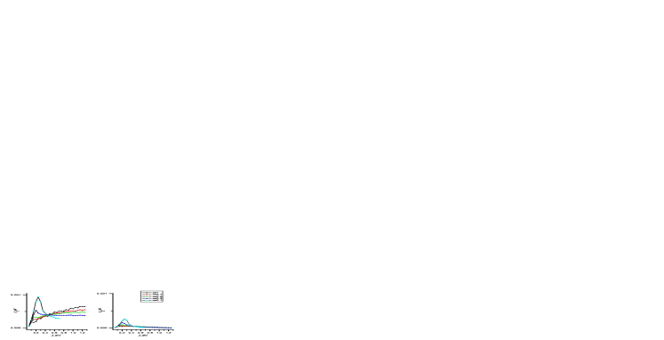
Figure 4: Dependence of the nearest-neighbor effective exchange integral $J_{1}$ and the next-nearest-neighboring one $J_{2}$ on the exchange coupling $J$ at $U\rightarrow\infty,W=0.5eV,n=0.06,S=5/2,T=0,$ for different values of concentration $x$.

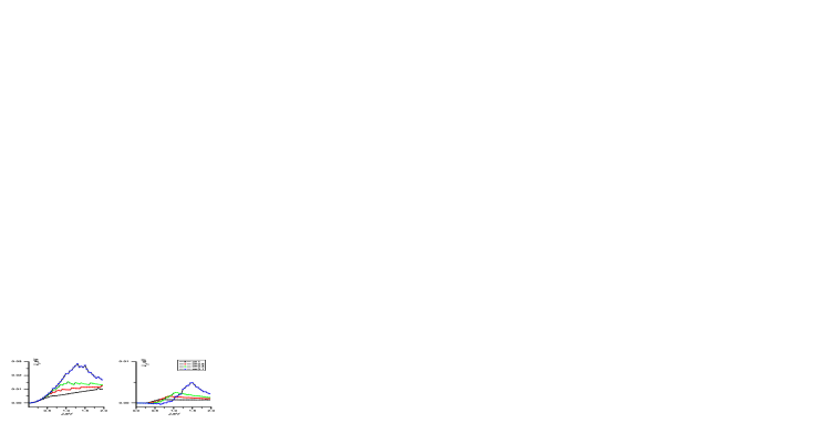
Figure 5: The same as in Fig. 4, but for $S=1/2$.

Figs. 4 and 5 represent the dependencies of the nearest-neighbor and the next-nearest-neighbor effective exchange interaction ($J_{1},J_{2}$) on the interband exchange coupling $J$, and for different concentrations $x$ and for two different spin values $S=5/2$ and $S=1/2$. In the strong coupling regime ($J>0.8$) of the concentrated system ($x=1$) only the short-range interaction ($J_{1}$) is important, the other interactions are small ($J_{2},J_{3},...$) Nolting3 . In the diluted and strong coupling case, however, the next-neighbor interaction $J_{1}$ becomes smaller (Fig. 4) than for $x=1$. In the low coupling regime ($J<0.1$) the results of the modified RKKY coincide with those of the conventional RKKY ($J_{1}\sim J^{2}$) (Fig. 4,5) which is nearly $x$-independent. The situation is much more complicated and non-monotonic in the intermediate coupling regime. Dilution may even lead to an enhanced value for the nearest-neighbor localized moment interaction $J_{1}$ compared with that for $x=1$ (Fig. 4,5). The self-consistent calculation of the effective exchange parameters $J_{1},J_{2},J_{3},..$ yields only a slight temperature-dependence of order $0.01$ meV or even less.

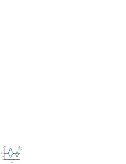
Figure 6: Electron DOS calculated with $U\rightarrow\infty,W=0.5eV,J=1.2eV,S=1/2,n=0.6$ a) $T=0$ for different values of the concentration $x$; b) $x=0.9$ for different values of the temperature $T$.

The electronic quasiparticle-DOS for different concentrations $x$ is shown in Fig. 6. There are two parts with different physical meanings. One part consists of correlated bands centered at $-JS/2$ and $J(S+1)/2$ due to the exchange interaction with magnetic atoms. The spectral weights of the two subbands are strongly temperature-dependent(see Fig. 6(b)). In the case of $T=0$ the spectral weight of the upper $\uparrow$ subband disappears, but however, is present in the $\downarrow$ spectrum. The second part around $\epsilon_{A}=0$ represents a non-correlated band being connected to the non-magnetic atoms (Fig. 2,6). This part of the spectrum is practically temperature independent.

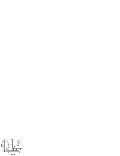
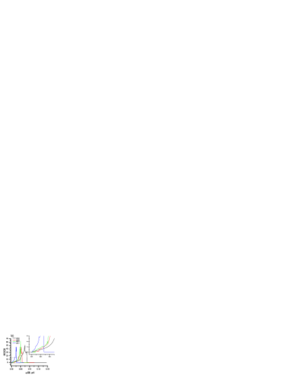
Figure 7: Magnon DOS calculated self-consistently by use of the VCA (a) and the Low Quadratic Approximation (b) with the same parameters as those in Fig. 6 for different values of the concentration $x$.

In Fig. 7 results for the magnon density of states are shown. Fig. 7(a) shows the magnon DOS in the VCA approximation (32) for the saturated ferromagnetic ground state. We see a typical consequence of dilution: a shift to the low energy side with decreasing concentration $x$ of magnetic atoms. The same is valid for the magnon DOS in the low quadratic approximation (Eq. 36) but there are some marked differences (Fig. 7(b)). Usually, in the case of weak magnon interaction (Fig. 7(a)), the magnon DOS near zero energy can be expressed as $DOS(E)=DE^{2}$, where $D$ is a stiffness parameter Furukawa . But for the strong magnon interaction, due to the disorder, the magnon DOS near zero energy has higher contributions, like as $DOS(E)=DE^{2}+KE^{3}$, where $K$ is the disorder parameter. These contributions are strongly modifying the magnon stiffness. For example, the huge low-energy part for low concentrations $x$ can be observed only for strong magnon interaction (inset of Fig. 7(b)). But in the VCA we have the normal $DOS(E)=DE^{2}$ behavior (inset of Fig. 7(a)). We conclude the same as in ref. Furukawa , that the disorder is strongly influencing the low energy magnon DOS.

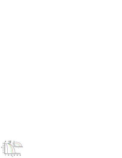
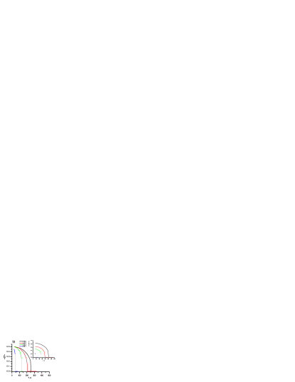
Figure 8: Self-consistent calculation of the dependence of the magnetization $\left\langle S^{z}\right\rangle$ on temperature by use of the VCA (a) and the Low Quadratic Approximation (b) with the same parameters as those in Fig. 6 for different values of the concentration $x$.

After the self-consistent calculation for finite temperatures, we obtain magnetization and the resulting value of the Curie temperature (Fig. 8(a), Fig. 8(b)). In Fig. 8(a), the magnetization curves are plotted which are obtained within the VCA for the magnon subsystem (Eq. 32). We see that the Curie temperature decreases with increasing dilution $1-x$. The same holds for the electron polarization (inset of Fig. 8(a)): $(n_{\uparrow}-n_{\downarrow})/n$.

The magnetization curves in Fig. 8(b) are determined within the low quadratic approach (Eq. 35,36) for the same parameters as for VCA in Fig. 8(a). Since this approach includes magnon scattering processes more realistically than the VCA, the Curie temperature for the same concentration $x$ of magnetic ions is lesser than that of VCA. For small $x$, the low quadratic approximation predicts first order ferromagnetic-paramagnetic transitions Gusev (dotted lines in Fig. 8(b)).

The explanation of this fact is based on predictions of the different approximations for the low energy part of the magnon DOS (see Fig. 7(a),7(b)). There was no report on first order transition in Ref. Tang . In our opinion this is related to the fact that spin disorder was treated in mean-field like approach, which is evidently comparable to our VCA results(see Fig. 8(a)), and which does not exhibit first order transition.

IV Discussion and Summary

There are many real materials where disorder plays an important role for electronic as well as magnetic properties (binary substitutional alloys, diluted magnetic semiconductors, perovskite manganese oxides, spin glass materials, transition metal dielectrics, etc.). Of course, these real systems are much more complicated than what the simple Kondo-lattice model predicts (complicated crystal lattice, multi-band structure, hybridization effects, spin-orbit coupling). However, we believe that the main microscopic mechanisms are well described in terms of the characteristic KLM features. The final goal is to make a quantitative description of those materials combining the present analytic model investigations with realistic ’ab initio’ calculations of the band structure as it was done previously for concentrated local-moment systems Hilbert ; Muller .

In this paper we discussed the influence of moment disorder on the electron and spin excitation spectra of the random KLM. Starting from an alloy analogy based on the exactly known zero-bandwidth limit of the KLM we applied a CPA procedure to find out the reaction of the electronic spectrum on the random mixture of magnetic and nonmagnetic atoms Nolting2 . The Hubbard term in the model Hamiltonian (1) helps to prevent states, which belong to double occupancies of lattice sites, to be ground states. The analytical expression for the electronic selfenergy has been used then to get the effective exchange integrals of the modified RKKY theory. The latter results from a mapping of the interband exchange onto an effective random Heisenberg model (Fig. 1) which was subsequently treated in the spirit of the well-known Tyablikov approximation. The disorder in the localized spin system turned out to be the most involved part of our study (Fig. 1). It was incorporated via the equation of motion method and the technique of configurational averaging. In order to decouple the higher-order averaged Green functions we used the approximation of independent fluctuations (29). The expression (31) for the averaged magnon Green function is generalized by using the structure factor of disordered distribution of magnetic atoms over a crystal lattice. Here we also used an approximation (35), identical to the low quadratic approach Fibich .

There is no direct interaction between the localized moments. Therefore, the collective order is caused by the indirect exchange interaction mediated by the itinerant band electrons. Consequently, the indirect momentum coupling strongly depends on electronic model parameters such as exchange coupling $J$ and band occupation $n$ (see Fig. 3). A further important parameter is of course the concentration of magnetic atoms $x$. The interactions found by modified RKKY resemble to those of the conventional RKKY only in the low coupling limit ($J\sim 0$). In the large coupling regime the long-range interaction transforms into short-range interaction (see Fig. 4,5), where only the nearest-neighbor interaction is important($J_{1}\neq 0,J_{2}\approx 0,J_{3}\approx 0,...$). But in the intermediate couplings we found that ( Fig. 4,5) the effective exchange interaction between the localized magnetic moments is strongly non-linear for small concentration $x$ of magnetic atoms. This effect was also considered in ref. Blackman ; DeGennes , and also recently discussed in ref. Singh1 ; Singh2 ; Kudrnovsky for diluted magnetic semiconductors. In ref. Kudrnovsky ; Sarma the influence of disorder on the RKKY interaction of two magnetic impurities was accounted for by a phenomenological damping factor. In general, this damping factor has to be calculated within the full Kondo-lattice model.

Another important finding is an influence of the disorder on the magnon excitations for small concentrations of magnetic atoms (Fig. 7). We found rather different results for the magnetic excitations in, respectively, VCA (Eq. 32, Fig. 7(a)) and the low quadratic approach Fibich (Eq. 36, Fig. 7(b)). It is clear that VCA yields too simple expressions for the magnon Green’s function (Eq. 36 and Eq. 31). Recently some treatments were proposed where the Kondo-lattice model is considered in the mean-field (VCA) approximation in order to explain real material properties Kudrnovsky ; Bouzerar1 ; Bouzerar2 taking into account only the dilution, while our results show that for small concentrations the disorder effects are also very important. Such effects play a crucial role for the understanding and controlling key-properties such as the Curie temperature. We see that disorder changes the magnon-DOS very drastically in particular for low energy excitations (Fig. 7(b)) which are decisive for the resulting values of the Curie temperature Furukawa ; Gusev .

We also note that there is another method to calculate the exchange interactions in ferromagnetic metals and alloys Liechtenstein . This method Liechtenstein ; Bruno works in the limit of infinite magnon wavelength. The MRKKY interaction does not have such a constraint. However, it is possible that for the disordered case the MRKKY theory (Eq. 10) has to be improved. The same leads true correct for the Callen equation (Eq. 12).

Some factors have not been included in our self-consistent calculation, for example, the environmental cluster effects for electron excitations. We are aware that this effect can modify the magnetic properties. These are currently being under investigation. Furthermore, as mentioned at the end of Sect. 2.1, the incorporation of the Hubbard type Coulomb interaction can be improved. This will be done in a forthcoming investigation which aims at the competition between band-magnetism due to the Hubbard interaction and local-moment magnetism due to the interband exchange $J$ of the Kondo-lattice model. The atomic-limit alloy analogy is then of course not an appropriate starting point.

In this paper we have restricted our considerations to the ferromagnetic ($J>0$) KLM, the standard “Kondo physics” ($J<0$) Burdin ; Mydosh is therefore excluded from the very beginning. The main goal was to work out the interplay between disorder and magnetic stability in diluted local-moment systems. We are aware that parts of our theory have to be refined to reproduce the standard “Kondo Physics”($J<0$).

V Acknowledgments

One of the authors (V.Bryksa) gratefully acknowledges financial support by the Graduate College of the Deutsche Forschungsgemeinschaft: ”Fundamentals and Functionality of Size and Interface Controlled Materials: Spin- and Optoelectronics”. We also thank Dr. Tang for helpful discussions and A. Sharma for critical reading of the manuscript.

References

- (1) W. Nolting, S. Rex and Jaya S. Mathi, J. Phys. C 9 (1996) 1301
- (2) D. Edwards, A. Green and K. Kubo, J. Phys. C 11 (1999) 2791
- (3) Yukitoshi Motome, Nobuo Fururawa, Phys. Rev. B 71 (2005) 014446
- (4) Toru Moriya, Spin Fluctuations in Itinerant Electron Magnetism (Berlin: Springer 1985) p 240
- (5) G. R. Stewart, Rev. of Mod. Phys. 56 (1984) 755
- (6) T. Sinova Jungwirth, J. Masek, J. Kucera, A. H. MacDonald, Rev. of Mod. Phys. 78 (2006) 809
- (7) A. I. Gusev, A. A. Rempel, A. J. Magerl, Disordered and Order in Strongly Nonstoichiometric Compounds (Berlin: Springer 2001) p 607
- (8) A. B. Harris, P. L. Leath, B. G. Nickel and R. J. Elliott, J. Phys. C 7 (1974) 1693
- (9) H. Dvey-Aharon, J. Phys. C 13 (1980) 197
- (10) A. Theumann, J. Phys. C 7 (1974) 2328
- (11) A. Theumann, R. A. Tahir-Kheli, Phys. Rev. B 12 (1975) 1796
- (12) R. A. Tahir-Kheli, Phys. Rev. B 6 (1972) 2808
- (13) Z. Gurskii, Condensed Matter Physics 3 (2000) 307
- (14) R. Johnston and D. Sherrington, J. Phys. C 15 (1982) 3757
- (15) D. Sherrington, J. Phys. C 41 (1978) 1321
- (16) H. Dvey-Aharon and M. Fibich, Phys. Rev. B 18 (1978) 3491
- (17) W. Nolting, G. Reddy, A. Ramakanth and D. Meyer, Phys. Rev. B 64 (2001) 155109
- (18) W. Nolting and A. M. Oles, J. Phys. C 13 (1980) 823
- (19) S. Hilbert and W. Nolting, Phys. Rev. B 70 (2004) 165203
- (20) R. C. Jones, J. Phys. C 4 (1971) 2903
- (21) R. Vlaming and D. Vollhardt, Phys. Rev. B 45 (1992) 4637
- (22) J. Schneider, V. Drehal, phys. stat. sol. (b) 68 (1975) 207
- (23) M. Potthoff, T. Herrmann, T. Wener and W. Nolting, phys. stat. sol. (b) 210 (1998) 199
- (24) R. J. Elliott, J. A. Krumhansl, P. L. Leath, Rev. of Mod. Phys. 46 (1974) 465
- (25) J. Kudrnovsky, I. Turek, V. Drchal, F. Maca, P. Weinberger and P. Bruno, Phys. Rev. B 69 (2004) 115208
- (26) G. Bouzerar and P. Bruno, Phys. Rev. B 66 (2002) 014410
- (27) J. A. Blackman and R. J. Elliott, J. Phys. C 2 (1969) 1670
- (28) J. A. Blackman and D. M. Esterling, N. F. Berk, Phys. Rev. B 4 (1971) 2412
- (29) P. G. De Gennes, Le Journal de Physique et le Radium 23 (1962) 630
- (30) R. Brout, Phys. Rev. 115 (1959) 824
- (31) H. B. Callen, Phys. Rev. 130 (1963) 890
- (32) G. Bouzerar, J. Kudrnovsky and P. Bruno, Phys. Rev. B 73 (2006) 024411
- (33) R. Bouzerar, G. Bouzerar and T. Ziman, Phys. Rev. B 73 (2006) 024411
- (34) Masao Takahashi, Phys. Rev. B 70 (2004) 035207
- (35) G. Tang, W. Nolting, Phys. Rev. B 75 (2007) 024426
- (36) Avinash Singh, Animesh Datta, K. Das Subrat and Vijay A. Singh, Phys. Rev. B 68 (2003) 235208
- (37) K. Das Subrat and Avinash Singh, Preprint cond-mat/0506523 (2005)
- (38) D. J. Priour, S. Sarma, Phys. Rev. Lett. 97 (2006) 127201
- (39) C. Santos and W. Nolting, Phys. Rev. B 66 (2002) 019901(E)
- (40) W. Nolting, T. Hickel, A. Ramakanth, G. G. Reddy and M. Lipowczan, Phys. Rev. B 70 (2004) 075207
- (41) W. Müller and W. Nolting, Phys. Rev. B 66 (2002) 085205
- (42) S. F. Edwards and R. C. Jones, J. Phys. C 4 (1971) 2109
- (43) T. Matsubara and F. Yonezawa, Prog. theor. Phys. 34 (1965) 871
- (44) A. I. Liechtenstein, M. I. Katsnelson, V.P. Antropov and V. A. Gubanov, J. Magn. Magn. Mater. 67 (1987) 65
- (45) M. Bruno, Phys. Rev. Lett. 90 (2003) 087205
- (46) S. Burdin and P. Fulde, Preprint cond-mat/0701598 (2007)
- (47) J. A. Mydosh, Spin glasses: an experimental introduction (Taylor & Francis 1993) p 256