An approximate version
of the Loebl-Komlós-Sós conjecture

Abstract

Loebl, Komlós, and Sós conjectured that if at least half of the vertices of a graph $G$ have degree at least some $k\in\mathbb{N}$, then every tree with at most $k$ edges is a subgraph of $G$. Our main result is an approximate version of this conjecture for large enough $n=|V(G)|$, assumed that $n=O(k)$.

Our result implies an asymptotic bound for the Ramsey number of trees. We prove that $r(\mathcal{T}_{k},\mathcal{T}_{m})\leq k+m+o(k+m)$, as $k+m\rightarrow\infty$.

1 Introduction

We explore how certain global assumptions on a graph $G$ ensure the existence of specific subgraphs. More precisely, we are interested in finding trees as (not necessarily induced) subgraphs. The main conjecture in our investigations makes, to this end, assumptions on the median degree of $G$.

Conjecture 1 (Loebl, Komlós, Sós [6]).

Let $k>0$. Then every graph on $n\in\mathbb{N}$ vertices of which at least $n/2$ have degree at least $k$, contains as subgraphs all trees with at most $k$ edges.

The original version for $k=n/2$ was formulated by Loebl, the generalisation to arbitrary $k$ is due to Komlós and Sós (see [6]). The $n=O(k)$ case of Conjecture 1 is often referred to as the dense case (otherwise the sparse case).

Our main result is an approximate version of Conjecture 1 for the dense case.

Theorem 2.

For every $\eta,q>0$ there is an $n_{0}\in\mathbb{N}$ such that for every graph $G$ on $n\geq n_{0}$ vertices and every $k\geq qn$ the following is true.

If at least ${n}/{2}$ vertices of $G$ have degree at least $(1+\eta)k$, then $G$ contains all trees with at most $k$ edges.

For arbitrary $k$, this has been conjectured by Ajtai, Komlós and Szemerédi in [1]. They gave a proof for the special case $k=n/2$.

The exact version, Conjecture 1, is trivial for stars, and for trees that consist of two stars with adjacent centres. Bazgan, Li, and Woźniak [2] have proved the conjecture for paths. The authors of the present paper proved in [10] the Loebl–Komlós–Sós conjecture for trees of diameter at most $5$.

In Loebl’s version with $k=n/2$, the conjecture has recently been proved by Zhao [14] for large enough graphs. Extending the methods of Zhao, and of the present paper, the full Loebl–Komlós–Sós conjecture has been proved very recently for the dense case by Hladký together with the first author [8], and independently, by Cooley [4].

A generalisation of an example due to Zhao [14] shows that the bound for the number of vertices of high degree in Conjecture 1 is asymptotically best possible. It cannot be replaced by $n/2-n/(k+1)$, whenever $k+1$ is even and divides $n$ (for bounds in other cases, see [10]).

To see this, construct a graph $G$ on $n$ vertices as follows. Divide $V(G)$ into $2n/(k+1)$ sets $A_{i}$, $B_{i}$, so that $|A_{i}|=(k-1)/2$, and $|B_{i}|=(k+3)/2$, for $i=1,\ldots,n/(k+1)$. Insert all edges inside each $A_{i}$, and insert all edges between each pair $A_{i}$, $B_{i}$. Now, consider the tree $T$ we obtain from a star with $(k+1)/2$ edges by subdividing each edge but one. Clearly, $T$ is not a subgraph of $G$.

An interesting folklore observation is the following. Assume that there is a counterexample to Conjecture 1 for the dense case that does not contain some tree of order $k+1$. By taking many copies of $G$, we could then construct a counterexample to Conjecture 1 for the sparse case.

The Ramsey number $r(H,H^{\prime})$ of two graphs, $H$ and $H^{\prime}$, is defined as the minimum integer $n$ such for every graph $G$ of order at least $n$ either $H$ is a subgraph of $G$, or $H^{\prime}$ is a subgraph of the complement $\bar{G}$ of $G$. Extending this definition, we denote by $r(\mathcal{H},\mathcal{H}^{\prime})$ the Ramsey number of two classes of graphs, $\mathcal{H}$ and $\mathcal{H}^{\prime}$, that is, $r(\mathcal{H},\mathcal{H}^{\prime})$ is the minimum integer $n$ such for every graph $G$ of order at least $n$ either each graph $H\in\mathcal{H}$ is a subgraph of $G$, or each graph $H^{\prime}\in\mathcal{H}^{\prime}$ is a subgraph of the complement $\bar{G}$ of $G$. We write $r(\mathcal{H})$ as shorthand for $r(\mathcal{H},\mathcal{H})$.

For $i\in\mathbb{N}$, let $\mathcal{T}_{i}$ denote the class of all trees of order $i$. Zhao’s result implies that the Ramsey number $r(\mathcal{T}_{k+1})\leq 2k$, for large $k$. Bounds for Ramsey numbers of trees have been studied for instance in [7]).

In the same way as the bound on $r(\mathcal{T}_{k+1})$ follows from the Loebl conjecture, one can deduce from Conjecture 1, if true, a bound on $r(\mathcal{T}_{k+1},\mathcal{T}_{m+1})$. Namely, for any colouring of the edges of the complete graph $K_{m+k}$ with two colours, either half of the vertices have degree $k$ in the subgraph induced by the first colour, or half of the vertices have degree $m$ in the subgraph induced by the second colour. So the Loebl–Komlós–Sós conjecture would then imply that $r(\mathcal{T}_{k+1},\mathcal{T}_{m+1})\leq k+m$. This upper bound has been conjectured in [6], and it is not difficult to see that the bound is best possible.

Using Theorem 2, we prove this to be asymptotically true.

Corollary 3.

$r(\mathcal{T}_{k+1},\mathcal{T}_{m+1})\leq k+m+o(k+m)$, as $k+m\rightarrow\infty$.

It is not difficult to see that the exact bound of $r(\mathcal{T}_{k+1},\mathcal{T}_{m+1})\leq k+m$ also follows from a positive answer to the Erdős–Sós conjecture. This well-known conjecture states that each graph with average degree greater than $k-1$ contains all trees with at most $k$ edges as subgraphs. For partial results on the Erdős–Sós conjecture, see e.g. [3, 11, 13]. Ajtai, Komlós, Simonovits and Szemerédi proved the Erdős–Sós conjecture for large $n$. (Unfortunately, a manuscript is not available yet.)

Our proof of Theorem 2 is inspired by the proof of the approximate version of the Loebl conjecture by Ajtai, Komlós and Szemerédi [1]. Here also, we use the regularity lemma followed by a Gallai-Edmonds decomposition of the reduced cluster graph. This enables us to find a certain substructure in the cluster graph, which contains a large matching, and captures the degree condition on $G$. The tree is then embedded mainly into the regular pairs corresponding to the matching edges.

We shall see that in the case that $k\geq n/2$, it is not difficult to obtain the same structure as in [1]. Our proof then follows [1], providing all details.

In the case that $k<n/2$, however, the situation is more complex. We will have to content ourselves with a less favourable structure in the cluster graph, which complicates the embedding of the tree. For a brief outline of the crucial ideas we then employ, see Section 3.1. The full proof is given in the remainder of Section 3.

Using similar ideas of proof, we extend Theorem 2 in a different direction. We pursue the question which other subgraphs are contained in our graph $G$ from Theorem 2.

Our third result asserts that we can replace the trees with bipartite graphs that may have a few more edges than trees.

Theorem 4.

For every $\eta,q>0$ and for every $c\in\mathbb{N}$ there is an $n_{0}\in\mathbb{N}$ so that for each graph $G$ on $n\geq n_{0}$ vertices and each $k\geq qn$ the following is true.

If at least ${n}/{2}$ vertices of $G$ have degree at least $(1+\eta)k$, then each connected bipartite graph $Q$ on $k+1$ vertices with at most $k+c$ edges is a subgraph of $G$.

In particular, the condition of Theorem 2 allows for embedding even cycles in $G$:

Corollary 5.

For every $\eta,q>0$ there is an $n_{0}\in\mathbb{N}$ so that for all graphs $G$ on $n\geq n_{0}$ vertices and each $k\geq qn$ the following is true.

If at least ${n}/{2}$ vertices of $G$ have degree at least $(1+\eta)k$, then $G$ contains all even cycles of length at most $k+1$.

Theorem 4 does not hold for $\eta=0$, as is witnessed by the following example. Take the complete graph on $k$ vertices and the empty graph on $k$ vertices. Connect these two graphs with a matching of order $k$. The graph we obtain satisfies the condition of the sharp version of Theorem 4, but does not contains the cycle of length $k+1$.

Also, the condition that $Q$ is bipartite is necessary. This can be seen by considering copies of the complete bipartite graph $K_{(1+\eta)k,(1+\eta)k}$. This graph satisfies the condition of Theorem 4, but all its subgraphs are bipartite.

Our paper is organised as follows. In Section 2.1, we introduce the regularity lemma and discuss some basic properties of regularity. Our tool for finding the desired structure of the cluster graph, Lemma 8, will be proved in Section 2.2. All of Section 3 is dedicated to the proof of our main result, Theorem 2.

In Section 4, we explore applications and generalisations of Theorem 2. Our asymptotic bound for Ramsey numbers of trees (Proposition 3) will be derived in Section 4.1. In Section 4.2, we prove Theorem 4.

2 Preliminaries

The purpose of this section is to introduce the two main tools used in the proofs of Theorem 2 and Theorem 4. The first of these tools is the well-known regularity lemma. The second is Lemma 8, which will give structural information on our graph $G$ from Theorem 2 (and Theorem 4). We derive it from the Gallai-Edmonds matching theorem.

2.1 Regularity

In this subsection, we introduce the notion of regularity, state Szemerédi’s regularity lemma, and review a few useful properties of regularity. All of this is well-known, so the advanced reader is invited to skip this section. For an instructive survey on the regularity lemma and its applications, consult [9].

Let us first go through some necessary notation. For a graph $G=(V,E)$, with $W\subseteq E$ and $S\subseteq V$, we will write $G-W$ for the subgraph $(V,E\setminus W)$ of $G$, and $G-S$ the subgraph of $G$ which is obtained by deleting all vertices of $S$ and all edges incident with vertices of $S$. For subsets $X$ and $Y$ of the vertex set $V(G)$, define $N_{Y}(X)$ as the set of all neighbours of $X$ in $Y\setminus X$. If $Y=V(G)$, then we omit the index $Y$ and write $N(X)$. A vertex $x\in V(G)$ is adjacent to the set $Y$ if $xy\in E(G)$ for some $y\in Y$. If $X$ and $Y$ are disjoint, then let $e(X,Y)$ denote the number of edges between $X$ and $Y$. The density of the pair $(X,Y)$ is $d(X,Y):=\frac{e(X,Y)}{|X||Y|}$.

A bipartite graph $G$ with partition classes $C_{1}$ and $C_{2}$ is called $\varepsilon$-regular if for all subsets $C_{1}^{\prime}\subseteq C_{1}$, $C_{2}^{\prime}\subseteq C_{2}$ with $|C_{1}^{\prime}|\geq\varepsilon|C_{1}|$ and $|C_{2}^{\prime}|\geq\varepsilon|C_{2}|$, it is true that $|d(C_{1},C_{2})-d(C^{\prime}_{1},C^{\prime}_{2})|<\varepsilon$.

A partition $C_{0}\cup C_{1}\cup\dots\cup C_{N}$ of $V(G)$ is called $(\varepsilon,N)$-regular, if

• $|C_{0}|\leq\varepsilon n$ and $|C_{i}|=|C_{j}|$ for $i,j\in\{1,\ldots,N\}$,

• all but at most $\varepsilon N^{2}$ pairs $(C_{i},C_{j})$ with $i\neq j$ are $\varepsilon$-regular.

We are now ready to state Szemerédi’s regularity lemma.

Theorem 6 (Regularity lemma, Szemerédi [12]).

For every $\varepsilon>0$ and $m_{0}\in\mathbb{N}$, there exist $M_{0},N_{0}\in\mathbb{N}$ so that every graph $G$ of order $n\geq N_{0}$ admits an $(\varepsilon,N)$-regular partition of its vertex set $V(G)$ with $m_{0}\leq N\leq M_{0}$.

Call the partition classes $C_{i}$ of $G$ clusters. Now, for each graph $G$, for each $(\varepsilon,N)$-regular partition of $V(G)$, and for any density $p$ define the cluster graph (sometimes called reduced graph) in the following standard way.

First, we construct an auxiliary graph $G_{p}$ obtained from $G$ by deleting all edges inside the clusters $C_{i}$, all edges that are incident with $C_{0}$, all edges between irregular pairs, and all edges between regular pairs $(C_{i},C_{j})$ of density $d(C_{i},C_{j})<p.$ Set $s:=|C_{i}|$, and observe that

$$|E(G-G_{p})|\leq N\frac{s^{2}}{2}+\varepsilon n^{2}+\varepsilon N^{2}s^{2}+\frac{N^{2}}{2}ps^{2}\leq(\frac{1}{2m_{0}}+2\varepsilon+\frac{p}{2})n^{2}.$$ (1)

Now, the cluster graph $H=H_{p}$ on the vertex set $\{C_{i}\}_{1\leq i\leq N}$ has an edge $C_{i}C_{j}$ for each pair $(C_{i},C_{j})$ of clusters that has positive density in $G_{p}$. We shall prefer to work with the weighted cluster graph $\bar{H}=\bar{H}_{p}$ which we obtain from $H$ by assigning weights

$$w(C_{i}C_{j}):=d(C_{i},C_{j})s$$

to the edges $C_{i}C_{j}\in E(H)$.

In the setting of weighted graphs, the (weighted) degree of a vertex $v$ is defined as

$${\rm d\bar{e}g}(v):=\sum_{u\in N(v)}w(vu),$$

and the degree into a subset $U\subseteq V(\bar{H})$, where we only count the weights of edges in $\{v\}\times U$, is denoted by ${\rm d\bar{e}g}_{U}(v)$. We shall adopt this notation for our weighted cluster graph $\bar{H}$. For a subset $X\subseteq C_{j}$, we write

$${\rm d\bar{e}g}_{X}(C_{i}):=\frac{e(X,C_{i})}{s}=d(X,C)|X|.$$

For a set $\mathcal{Y}$ of subsets of distinct clusters from $G_{p}-C_{i}$, we shall write ${\rm d\bar{e}g}_{\mathcal{Y}}(C_{i})$ for $\sum_{Y\in\mathcal{Y}}{\rm d\bar{e}g}_{Y}(C_{i})$.

We shall often use edges of $\bar{H}$ to represent the respective subgraph of $G_{p}$, or sometimes its vertex set. For example, an edge $e=CD\in E(\bar{H})$, might refer to the subgraph of $G_{p}$ induced by $C\cup D$, or to $C\cup D$ itself. And for a set $U\subseteq C\cup D$, we sometimes use the shorthand $e\cap U$ for $(C\cup D)\cap U$.

Let us review some basic properties of $G_{p}$ and $\bar{H}$. Let $C,D\in V(\bar{H})$: We call a set $D^{\prime}\subseteq D$ significant, if $|D^{\prime}|\geq\varepsilon s$. A vertex $v\in C$ is called typical to a significant set $D^{\prime}$ if $\deg_{D^{\prime}}(v)\geq(d(C,D)-\varepsilon)|D^{\prime}|$. Observe that

$$\text{at most }\varepsilon s\text{ vertices of }C\text{ are not typical to a given significant set }D^{\prime}.$$ (2)

Similarly, we have that

$$\text{all but at most }\varepsilon s\text{ vertices $v$ of }C\text{ have degree }\deg_{G_{p}}(v)\leq{\rm d\bar{e}g}(C)+\varepsilon n.$$ (3)

For proofs of (2) and (3), we refer the reader to [1].

Also, almost all vertices of any cluster $C\in V(\bar{H})$ are typical to almost all significant sets, in the following sense.

If $\mathcal{Y}$ is a set of significant subsets of clusters in $V(\bar{H})$, then

$$|\{Y\in\mathcal{Y}:\;v\text{ is typical to }Y\}|\geq(1-\sqrt{\varepsilon})|\mathcal{Y}|,$$ (4)

for all but at most $\sqrt{\varepsilon}s$ vertices $v\in C$.

To see this, assume that the set $C^{\prime}\subseteq C$ of vertices not satisfying (4) is larger than $\sqrt{\varepsilon}s$. Then

$$\sum_{Y\in\mathcal{Y}}|\{v\in C:\;v\text{ is not typical to }Y\}|\geq \ \sum_{v\in C^{\prime}}|\{Y\in\mathcal{Y}:\;v\text{ is not typical to }Y\}|$$

$$\geq \ |C^{\prime}|\sqrt{\varepsilon}|\mathcal{Y}|$$

$$> \ \varepsilon s|\mathcal{Y}|.$$

Thus there is a $Y\in\mathcal{Y}$ such that more than $\varepsilon s$ vertices in $C$ are not typical to $Y$, a contradiction to (2).

2.2 The matching

The main interest in this subsection is Lemma 8, which will give us important structural information on the cluster graph $H$ that corresponds to the graph $G$ from Theorem 2 (or later Theorem 4). Lemma 8 appeared in [1] but only a weaker variant was proved.

For the proof of Lemma 8, we need a simplified version of the Gallai-Edmonds matching theorem, a proof of which can be found for example in [5, p. 41].

A $1$-factor, or perfect matching, of a graph $G$ is a $1$-regular spanning subgraph of $G$. We call $G$ factor-critical, if for each $v\in V(G)$, there exists a perfect matching of $G-v$.

Theorem 7 (Gallai, Edmonds).

Every graph $G$ contains a set $S\subseteq V(G)$ so that each component of $G-S$ is factor-critical, and so that there is a matching in $G$ that matches the vertices of $S$ to vertices of different components of $G-S$.

We are now ready for one of the key tools in the proof of Theorem 2. Recall that we often conveniently use $M$ to represent $V(M)$.

Lemma 8.

Let $\bar{H}$ be a weighted graph on $N$ vertices, and let $K\in\mathbb{R}$. Let $L$ be the set of those vertices $v\in V(\bar{H})$ with ${\rm d\bar{e}g}(v)\geq K$. If $|L|>N/2$, then there are two adjacent vertices $v_{A},v_{B}\in L$, and a matching $M$ in $\bar{H}$ such that one of the following holds.

1. $M$ covers $N(\{v_{A},v_{B}\})$,

2. $M$ covers $N(v_{A})$, and ${\rm d\bar{e}g}_{M\cup L}(v_{B})\geq K/2$. Moreover, each edge in $M$ has at most one endvertex in $N(v_{A})$.

Proof.

Observe that we may assume that $Y:=V(\bar{H})\setminus L$ is independent. (In fact, otherwise we simply delete the edges in $E(Y)$, which will not affect the degree of the vertices in $L$.) Now, Theorem 7 applied to the unweighted version of $\bar{H}$ yields a set $S\subseteq V(\bar{H})$. Among all matchings $M^{\prime}$ satisfying the conclusion of Theorem 7 with $S$, choose $M^{\prime}$ so that it contains a maximal number of vertices of $Y$.

Set $L^{\prime}:=L\setminus S$. We shall show that either (a) holds or $L^{\prime}$ is independent. Suppose there is an edge $uv$ with endvertices $u,v\in L^{\prime}$. Then $uv$ lies in some component $C$ of $\bar{H}-S$. If $V(C)\cap V(M^{\prime})=\emptyset$, let $M^{\prime\prime}$ be a $1$-factor of $C-u$, and if $V(C)\cap V(M^{\prime})=\{x\}$, then let $M^{\prime\prime}$ be a $1$-factor of $C-x$. In either case (a) holds for $v_{A}v_{B}=uv$ with $M:=M^{\prime}\cup M^{\prime\prime}$. So, from now on, we assume that $L^{\prime}$ is independent.

Then, each edge of $\bar{H}$ that is not incident with $S$ has one endvertex in $L^{\prime}$, and one in $Y$. Consider any component $C$ of $\bar{H}-S$. Since $C$ is factor-critical, we have that $|(C-u)\cap Y|=|(C-u)\cap L^{\prime}|$, for every $u\in V(C)$. Hence, $C$ consists of only one vertex, and so must every component of $\bar{H}-S$.

Figure 1: The graph $\bar{H}$ with the matching $M^{\prime}$, and sets $L$, $S$ and $Y$.

Denote by $X$ the subset of $Y$ that is not covered by $M^{\prime}$. Set $\tilde{L}:=N(L^{\prime})\cap L\subseteq S$ (see Figure 1). Now, if there is a vertex $v_{B}\in\tilde{L}$ whose weighted degree into $\bar{H}-X$ is at least $K/2$, then $v_{B}$, together with any of its neighbours $v_{A}$ in $L^{\prime}$, satisfies (b) with $M=M^{\prime}$. So, we may assume that for each $u\in\tilde{L}$,

$${\rm d\bar{e}g}_{\bar{H}-X}(u)<K/2,$$ (5)

and hence ${\rm d\bar{e}g}_{X}(u)\geq K/2$.

On the other hand, ${\rm d\bar{e}g}_{\tilde{L}}(w)<K$ for each $w\in X$. Thus, by double (weighted) edge-counting, it follows that

$$|X|\geq\frac{|\tilde{L}|}{2}.$$ (6)

Set $S^{\prime}:=S\cap Y$. By (5), the total weight of the edges in $E(\tilde{L}\cup S^{\prime},L^{\prime})$ is less than $|\tilde{L}|K/2+|S^{\prime}|K$, while each vertex of $L^{\prime}$ has weighted degree at least $K$ into $\tilde{L}\cup S^{\prime}$. Thus, again by double edge-counting, and by (6),

$$|X|+|S^{\prime}|\geq\frac{|\tilde{L}|}{2}+|S^{\prime}|>|L^{\prime}|.$$ (7)

Furthermore, since $Y$ is independent, $M^{\prime}$ matches $S^{\prime}\subseteq Y$ to $L^{\prime}$. Thus $|L^{\prime}|\geq|S^{\prime}|+|L\setminus M^{\prime}|$, and so, by (7),

$$|X|>|L\setminus M^{\prime}|.$$

Since $|L|>\frac{N}{2}$, this implies that $M^{\prime}$ contains an edge $uv$ with both $u,v\in L$. We may assume that $v\in L^{\prime}$ and $u\in\tilde{L}$. By (5), $u$ has a neighbour $w$ in $X$. Hence, the matching $M^{\prime}\cup\{uw\}\setminus\{uv\}$ covers more vertices of $Y$ than $M^{\prime}$ does, a contradiction to the choice of $M^{\prime}$. ∎

Note that in the case $K\geq N/2$ the situation in Lemma 8 is less complicated. In that case, observe that clearly $|S|\leq|V(\bar{H}-S)|$. So, either $|S|=|V(\bar{H}-S)|$ (in which case conclusion (a) of Lemma 8 holds), or there is a component $C$ of $\bar{H}-S$ that has more than one vertex. Thus, as $C$ is factor-critical, there exists an edge in $C\cap(L^{\prime}\times L^{\prime})$, and (a) holds again. In the case $k\geq n/2$, this observation simplifies our proof of Theorem 2 considerably, as then only the simplest case needs to be treated.

3 Proof of Theorem 2

The organisation of this section is as follows. The first subsection is devoted to an outline of our proof, highlighting the main ideas, leaving out all details. In Subsection 3.2, assuming that we are given a host graph $G$ and a tree $T^{*}$ as in Theorem 2, we shall first apply the regularity lemma to $G$. We then use Lemma 8 to find a suitable matching of the corresponding weighted cluster graph $\bar{H}$, which will facilitate the embedding of $T^{\ast}$.

We shall prepare $T^{\ast}$ for this by cutting it into small pieces in Subsections 3.3 and 3.4. Then, in Subsection 3.5, we partition the matching given by Lemma 8, according to the decomposition of the tree $T^{\ast}$. In Subsection 3.6, we expose tools that we need for our embedding. What remains is the actual embedding procedure, which we divide into the two cases given by Lemma 8, and treat separately in Subsections 3.7 and 3.8.

3.1 Overview

In this subsection, we shall give an outline of our proof of Theorem 2. So, assume that we are given $\eta>0$ and $q>0$. The regularity lemma applied to parameters depending on $\eta$ and $q$ yields an $n_{0}\in\mathbb{N}$. Now, let $n\geq n_{0}$, let $k\geq qn$, let $G$ be a graph of order $n$ that satisfies the condition of Theorem 2, and let $T^{\ast}$ be a tree with $k$ edges. We wish to find a subgraph of $G$ that is isomorphic to $T^{\ast}$, i.e. we would like to embed $T^{\ast}$ in $G$.

In order to do so, consider the weighted cluster graph $\bar{H}$ corresponding to $G$ that is given by the regularity lemma. Denote by $L\subseteq V(\bar{H})$ the set of those clusters that have degree at least $(1+\pi^{\prime})k$ in $\bar{H}$, where $\pi^{\prime}=\pi^{\prime}(\eta,q)>0$. The weighted cluster graph $\bar{H}$ inherits properties from $G$ resulting in the fact that $|L|>|V(\bar{H})|/2$. Apply Lemma 8 to $\bar{H}$ and $K:=(1+\pi^{\prime})k$ which yields vertices $A,B\in V(\bar{H})$ and a matching $M$. The rest of our proof will be divided into two cases, corresponding to the two possible conclusions (a) and (b) of Lemma 8.

If the output of Lemma 8 is Case (a), then we shall decompose $T^{*}$ into small subtrees (of order much below $\eta k$) and a small set $SD$ of vertices (of constant order in $n$), so that between any two of our subtrees lies a vertex from $SD$ (the name $SD$ stands for ‘seeds’). In fact, $SD$ is the disjoint union of two sets $SD^{A}$ and $SD^{B}$, and each tree $T$ of $T^{\ast}-SD$ is adjacent to only one of these two sets, that is, either $N(SD^{A})\cap V(T)=\emptyset$ or $N(SD^{B})\cap V(T)=\emptyset$. Denote the set of trees adjacent to $SD^{A}$ by $\mathcal{T}_{A}$, and the set of trees adjacent to $SD^{B}$ by $\mathcal{T}_{B}$. The formal definition of $SD$, $\mathcal{T}_{A}$ and $\mathcal{T}_{B}$ can be found in Section 3.3.

Next, in Section 3.5, we partition the matching $M$ from Lemma 8 into $M_{A}$ and $M_{B}$. This is done in a way so that ${\rm d\bar{e}g}_{M_{A}}(A)$ is large enough so that $F_{A}:=\bigcup\mathcal{T}_{A}$ fits into $M_{A}$, and ${\rm d\bar{e}g}_{M_{B}}(B)$ is large enough so that $F_{B}:=\bigcup\mathcal{T}_{B}$ fits into $M_{B}$.

Finally, in Section 3.7, we embed $SD^{A}$ in $A$ and $SD^{B}$ in $B$ and use the regularity of the edges in $\bar{H}$ to embed the small trees of $\mathcal{T}_{A}\cup\mathcal{T}_{B}$, one after the other, levelwise, into $M_{A}\cup M_{B}$. The order of this embedding procedure will be such that the already embedded part of $T^{\ast}$ is always connected.

Moreover, the structure of our decomposition of $T^{\ast}$, and the fact that we embed the trees from $\mathcal{T}_{A}\cup\mathcal{T}_{B}$ in the matching edges, ensures that the predecessor of any vertex $r\in SD^{A}\cup SD^{B}$ is embedded in a cluster that is adjacent to $A$, respectively to $B$ (in which we wish to embed $r$). This enables us to embed all of $SD$ in $A\cup B$, as planned.

An important detail of our embedding technique is that we shall always try to balance the embedding in the matching edges, in the sense that the used part of either endcluster should have about the same size. We only allow for an unbalanced embedding if the degree of $A$ resp. $B$ into one of the endclusters of the concerned edge is already ‘exhausted’ (cf. Property $(\diamond)$ in Section 3.6). In practice, this means that whenever we have the choice into which endcluster of an edge $e\in M$ we embed the root of some tree of $\mathcal{T}_{A}\cup\mathcal{T}_{B}$, we shall choose the side carefully.

In this manner, we can ensure that all of $T^{\ast}$ will fit into $M$ (or more precisely into the corresponding subgraph of $G$). This finishes the embedding of $T^{\ast}$ in Case (a) of Lemma 8.

In Case (b) of Lemma 8, it is not possible to partition the matching $M$ into $M_{A}$ and $M_{B}$ so that $F_{A}$ fits into $M_{A}$ and $F_{B}$ fits into $M_{B}$, as in Case (a). More precisely, for any partition of $M$ into $M_{A}$ and $M_{B}$, if ${\rm d\bar{e}g}_{M_{A}}(A)$ allows for the embedding of a forest of order $t$, say, in $M_{A}$, then ${\rm d\bar{e}g}_{M_{B}\cup L}(B)$ only guarantees for the embedding of a forest of order at most $(k-t)/2$ in the subgraph of $G_{p}$ induced by $M_{B}$ and the edges incident with $L^{\prime}$, where $L^{\prime}:=L\setminus M$. For more details on this, see Lemma 9.

We use a combination of two strategies to overcome this problem. Firstly, we shall embed $T^{\ast}$ in two phases, leaving for the second phase some subtrees that are (each) adjacent to only one vertex from $SD$. Secondly, we shall embed some of the trees from $\mathcal{T}_{B}$ in part of the matching reserved for $F_{A}$. This means that we ‘switch’ some of our trees to $\mathcal{T}_{A}$.

Let us explain the two strategies in more detail. We modify our sets $\mathcal{T}_{A},\mathcal{T}_{B}$, in the following way. Denote by $\bar{\mathcal{T}}_{A}$ the set of those trees from $\mathcal{T}_{A}$ that are adjacent to only one vertex from $SD^{A}$, and similarly define $\bar{\mathcal{T}}_{B}$. (Observe that $T^{*}$ remains connected after deleting any tree in $\bar{\mathcal{T}}_{A}\cup\bar{\mathcal{T}}_{B}$.)

We may assume that

$$|V(\bigcup\bar{\mathcal{T}}_{A})|\geq|V(\bigcup\bar{\mathcal{T}}_{B})|.$$

Finally, set $\mathcal{T}^{\prime}:=(\mathcal{T}_{A}\cup\mathcal{T}_{B})\setminus(\bar{\mathcal{T}}_{A}\cup\bar{\mathcal{T}}_{B})$. Our plan now is to first embed the trees from $\mathcal{T}^{\prime}\cup\bar{\mathcal{T}}_{B}$ together with the vertices from $SD$ and to postpone the embedding of $\bar{F}_{A}:=\bigcup\bar{\mathcal{T}}_{A}$ to a later stage. As the part of the tree embedded in the first phase is connected, we avoid the difficulty of having to connect already embedded parts of $T^{\ast}$ in the second phase.

Now, we shall partition $M$ into $M_{f}$ and $\bar{M}_{B}$ so that ${\rm d\bar{e}g}_{M_{f}}(A)$ allows for the embedding of $\bigcup\mathcal{T}^{\prime}$, and ${\rm d\bar{e}g}_{\bar{M}_{B}\cup L}(B)$ allows for the embedding of $\bar{F}_{B}:=\bigcup\bar{\mathcal{T}}_{B}$. This actually means that the place we reserved for the embedding of $F_{B}-\bar{F}_{B}$ lies in $M_{f}$. Therefore, we shall ‘switch’ this forest to $\mathcal{T}_{A}$ (which is the second of our strategies).

Let us explain what we mean by switching. For each tree $T\in\mathcal{T}_{B}\setminus\bar{\mathcal{T}}_{B}$, delete all vertices from $T$ that are adjacent to $SD^{B}$ in $T^{\ast}$ and add them to $SD^{A}$. Put the components of what remains of $T$ into $\mathcal{T}_{A}$. Denote the thus enlarged $SD^{A}$ by $~{}\overline{\!\!S~{}~{}}\!\!\!\!D^{A}$ and set $~{}\overline{\!\!S~{}~{}}\!\!\!\!D:=~{}\overline{\!\!S~{}~{}}\!\!\!\!D^{A}\cup SD^{B}$.

After switching all trees $T\in\mathcal{T}_{B}\setminus\bar{\mathcal{T}}_{B}$, denote by $\mathcal{T}_{f}$ the (enlarged) set $\mathcal{T}_{A}\setminus\bar{\mathcal{T}}_{A}$. That is, $\mathcal{T}_{f}$ consists of all trees from the original $\mathcal{T}_{A}\setminus\bar{\mathcal{T}}_{A}$, together with all trees we generated by switching. It will be easy to verify that the switching procedure does not increase too much the number of seeds.

Also, each tree from $\mathcal{T}_{f}$ and $\bar{\mathcal{T}}_{A}$ is adjacent only to the enlarged $~{}\overline{\!\!S~{}~{}}\!\!\!\!D^{A}$, and each tree from $\bar{\mathcal{T}}_{B}$ is still adjacent only to $SD^{B}$. For details on the switching procedure, consult Section 3.4.

It remains to embed $T^{*}$ in $G$, which is done in Section 3.8. We first embed the vertices from $~{}\overline{\!\!S~{}~{}}\!\!\!\!D^{A}\cup SD^{B}$ in $A\cup B$, embed $F_{f}:=\bigcup\mathcal{T}_{f}$ in $M_{f}$, and embed part of $\bar{\mathcal{T}}_{B}$ in $\bar{M}_{B}$, in the same way as in Case (a). In a second phase, we embed the remaining trees from $\bar{\mathcal{T}_{B}}$ into edges of $H$ that are incident with $L^{\prime}$. For each tree, we are able to find a free space in a suitable edge because of the high degree of the clusters from $L^{\prime}$.

In the remaining third phase we wish to embed $\bar{F}_{A}$. We shall now use all of $M$, forgetting about the partition into $M_{f}$ and $\bar{M}_{B}$. The neighbours of the trees from $\bar{\mathcal{T}}_{A}$ in $~{}\overline{\!\!S~{}~{}}\!\!\!\!D^{A}$ have already been embedded in the first phase. Having chosen their images carefully then, ensures that now they have still large enough degree into what is not yet used of $M$. Hence, there is enough place for $\bar{F}_{A}$ in $M$.

Also, it is essential here that each edge of $M$ meets $N(A)$ in at most one cluster. The reason is that parts of these clusters might have been used in the first and second phases of the embedding. So, some of the edges involved might be unbalanced, in the sense above, because e. g. the degree of $B$ was such that we were not able to choose the endcluster in which we embedded the roots of the trees from $\bar{\mathcal{T}}_{B}$. However, as each edge of $M$ has at most one endcluster in $N(A)$, it is irrelevant whether the embedding is balanced or not in these edges.

The embedding itself of $\bar{F}_{A}$ is done as before. This finishes the sketch of our proof in Case (b).

3.2 Preparations

We shall now prove Theorem 2. First of all, we fix a few constants depending on $\eta$ and $q$. Set

$$\pi:=\min\{\eta,q\},\quad\varepsilon:=\frac{\pi^{7}q}{25\cdot 10^{7}}\quad\text{ and }\quad m_{0}:=\frac{500}{q\pi^{3}}.$$

The regularity lemma (Theorem 6) applied to $\varepsilon$, and $m_{0}$ yields natural numbers $M_{0}$ and $N_{0}$. Fix

$$\beta:=\frac{\varepsilon}{M_{0}},\quad p:=\frac{\pi^{3}q}{250}\quad\text{ and }\ \ \ n_{0}:=\max\left\{N_{0},\frac{64M_{0}}{\beta p}\right\}.$$

Thus our constants satisfy the following relations

$$\frac{1}{n_{0}}\ \ll\ \beta\ \ll\ \varepsilon\ \ll\ \frac{1}{m_{0}}\ <\ p\ \ll\ \pi\ \leq\ q,$$

where $a\ \ll\ b$ stands for the fact that $a<\frac{\pi}{100}b$.

In particular, $p$ satisfies

$$4\varepsilon+\frac{1}{m_{0}}<p.$$ (8)

Let $n\geq n_{0}$, let $k\geq qn$, and let $G$ be a graph of order $n$ which has at least $\frac{n}{2}$ vertices of degree at least $(1+\eta)k$. Suppose $T^{\ast}$ is a tree of order $k+1$. Our aim is to find an embedding $\varphi:V(T^{\ast})\to V(G)$ that preserves adjacency.

Now, by Theorem 6 there exists an $(\varepsilon,N)$-regular partition of $V(G)$, with $m_{0}\leq N\leq M_{0}$. As in Section 2.1, let $G_{p}$ be the subgraph of $G$ that preserves exactly the edges between regular pairs of density at least $p$.

By (1) and by (8),

$$|E(G-G_{p})|<pn^{2}\leq\frac{\pi^{3}}{250}kn.$$

Thus, for all but at most $\frac{\pi^{2}}{50}n$ vertices $v$, we have that $\deg_{G_{p}}(v)\geq\deg_{G}(v)-\frac{\pi}{5}k$. Hence,

$$G_{p}\text{\em has at least }\left(1-\frac{\pi^{2}}{25}\right)\frac{n}{2}\text{\em vertices of degree at least }\left(1+\frac{4\pi}{5}\right)k.$$

Let $\bar{H}=\bar{H}_{p}$ be the weighted cluster graph corresponding to $G_{p}$. Denote by $L$ the set of those clusters in $V(\bar{H})$ that contain more than $\varepsilon s$ vertices of degree at least $(1+\frac{4\pi}{5})k$ in $G_{p}$. A simple calculation shows that $|L|>(1-\frac{\pi^{2}}{5})\frac{N}{2}$.

Now, delete $\min\{\pi^{2}N/5,|V(\bar{H})\setminus L|\}$ clusters in $V(\bar{H})\setminus L$ to obtain a subgraph of the cluster graph $\bar{H}$. As this subgraph is very similar (or identical) to $\bar{H}$, in the rest of the text we shall denote it as well by $\bar{H}$. So from now on, by $\bar{H}$, we shall always refer to this subgraph. Each vertex in $\bigcup L$ drops its degree by at most $\frac{\pi^{2}}{5}Ns\leq\frac{\pi k}{5}$. Thus, by (3), each $X\in L$ has degree

$${\rm d\bar{e}g}_{\bar{H}}(X)\geq(1+\frac{3\pi}{5})k-\varepsilon n>(1+\frac{\pi}{5})k.$$ (9)

Then Lemma 8 applied to $\bar{H}$ and $K:=(1+\frac{\pi}{5})k$ yields an edge $AB\in E(\bar{H})$ with $A,B\in L$, together with a matching $M^{\prime}$ of $\bar{H}$, which satisfy (a) or (b) of Lemma 8. Obtain $M$ from $M^{\prime}$ by deleting all edges from $M^{\prime}$ that are incident with $A$ or with $B$. If $AA^{\prime},BB^{\prime}\in M^{\prime}$, then $M$ misses $A$, $A^{\prime}$, $B$, and $B^{\prime}$, thus at most three clusters from $N(A)$, resp. from $N(B)$. In Case (a) of Lemma 8, we calculate that

$$\min\{{\rm d\bar{e}g}_{M}(A),{\rm d\bar{e}g}_{M}(B)\} \geq\ (1+\frac{\pi}{5})k-\frac{3n}{N}$$

$$\geq\ (1+\frac{\pi}{5}-\frac{3}{qm_{0}})k$$

$$\geq\ (1+\frac{\pi}{10})k.$$ (10)

Similarly, in Case (b) it follows that

$${\rm d\bar{e}g}_{M}(A)\geq(1+\frac{\pi}{10})k\ \ \text{ and }\ \ {\rm d\bar{e}g}_{M\cup L}(B)\geq(1+\frac{\pi}{10})\frac{k}{2}.$$ (11)

Thus, for the remainder of our proof of Theorem 2 we shall work with the assumption that there is a matching $M$ of $\bar{H}$ and vertices $A,B\notin V(M)$ so that

1. ${\rm d\bar{e}g}_{M}(A),{\rm d\bar{e}g}_{M}(B)\geq(1+\frac{\pi}{10})k$, or

2. ${\rm d\bar{e}g}_{M}(A)\geq(1+\frac{\pi}{10})k$, ${\rm d\bar{e}g}_{M\cup L}(B)\geq(1+\frac{\pi}{10})\frac{k}{2}$, and each cluster in $N(A)$ meets a different edge of $M$.

We shall refer to these two cases as ‘Case 1’ and ‘Case 2’, respectively. We will embed the tree $T^{*}$ in the subgraph of $G_{p}$ corresponding to $\bar{H}$, using two different strategies in Case 1 and in Case 2.

3.3 Partitioning the tree

In this section, we shall cut our tree into small pieces. More precisely, we shall define a set $SD\subseteq V(T^{\ast})$, and sets $\mathcal{T}_{A}$ and $\mathcal{T}_{B}$ of disjoint small subtrees of $T^{\ast}$ which are connected through the vertices from $SD$. Moreover, $SD$ together with the union of all trees from $\mathcal{T}_{A}\cup\mathcal{T}_{B}$ will span $T^{\ast}$.

Fix a vertex $R$ of $T^{\ast}$ as the root and regard $T^{*}$ as a poset having $R$ as the minimal element. For a vertex $x$ of a subtree $T\subseteq T^{\ast}$, denote by $T(x)$ the subtree of $T$ induced by $x$ and all vertices $y$ greater than $x$ in the tree-order of $T^{\ast}$. (That is, $T(x)$ contains all vertices $y$ such that the path between the root $R$ and $y$ contains the vertex $x$.) If $R\notin V(T)$, then define the seed $sd(T)$ of $T$ as the maximal vertex of $T^{\ast}$ which is smaller than every vertex of $T$.

Our sets $SD=SD^{A}\cup SD^{B}$, $\mathcal{T}_{A}$ and $\mathcal{T}_{B}$ will satisfy:

1. $SD^{A}\cap SD^{B}=\emptyset$,

2. $R\in SD^{A}$, and $r\in SD$ lies at even distance to $R$ if and only if $r\in SD^{A}$,

3. $\mathcal{T}_{A}\cup\mathcal{T}_{B}$ consists of the components of $T^{\ast}-SD$,

4. $|V(T)|\leq\beta k$, and $sd(T)\in SD$, for each $T\in\mathcal{T}_{A}\cup\mathcal{T}_{B}$,

5. $\max\{|SD^{A}|,|SD^{B}|\}\leq\frac{2}{\beta}$, and

6. $e_{T^{*}}(V(F_{A}),SD^{B})=0$, and $e_{T^{*}}(V(F_{B}),SD^{A})=0$,

where $F_{A}:=\bigcup_{T\in\mathcal{T}_{A}}T$ and $F_{B}:=\bigcup_{T\in\mathcal{T}_{B}}T$ are the forests spanned by $\mathcal{T}_{A}$ and $\mathcal{T}_{B}$.

Let us first define $SD$. To this end, we shall inductively find vertices $x_{i}$, and define auxiliary trees $T^{i}\subseteq T^{\ast}$. Set $T^{0}:=T^{\ast}$.

In step $i\geq 1$, let $x_{i}\in V(T^{*})$ be a maximal vertex in the tree-order of $V(T^{i-1})$ with

$$|V(T^{i-1}(x_{i}))|>\beta k,$$ (12)

as illustrated in Figure 2(a), and define

$$T^{i}:=T^{i-1}-(T^{i-1}(x_{i})-x_{i}).$$

Hence,

$$|V(T^{i-1})|-|V(T^{i})|>(\beta k-1).$$ (13)

(a) Suppose that $x_{1},x_{4},x_{5},x_{7},x_{9}$ are in $T^{i-1}(x_{i})$.

(b) Say $x_{i}\in A^{\prime}$. Then $x_{5},x_{9}\in A^{\prime}$ and $x_{1},x_{4},x_{7}\in B^{\prime}$, which we mark by circles and squares respectively.

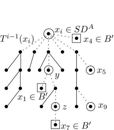
(c) We add $y$ and $z$ to $A(T)$. Then $T^{i-1}(x_{i})-SD\subseteq\mathcal{T}_{A}$.

Figure 2: Phases of the partition of $T^{\ast}$.

If there is no vertex satisfying (12), then set $x_{i}:=R$, and stop the definition process. Say our process stops in some step $j$. Let $A^{\prime}$ be the set of all $x_{i}$, $i\leq j$, with even distance to the root $R$, and let $B^{\prime}$ be the set of all other $x_{i}$.

Then, by (13) and by the definition of $n_{0}$,

$$j-1\leq\frac{|V(T^{*})|}{\beta k-1}=\frac{k+1}{\beta k-1}\leq\frac{3}{2\beta}.$$

Hence,

$$|A^{\prime}\cup B^{\prime}|\leq\frac{2}{\beta}.$$ (14)

For the sake of condition (VI), we shall now add a few more vertices to our sets $A^{\prime}$ and $B^{\prime}$, which will result in the desired $SD$.

Let $\mathcal{C}$ be the set of the components of $T^{\ast}-(A^{\prime}\cup B^{\prime})$. For each $T\in\mathcal{C}$ with $sd(T)\in A^{\prime}$, denote by $A(T)$ the set of vertices of $T$ that are adjacent to $B^{\prime}$. Similarly, if $sd(T)\in B^{\prime}$, then denote by $B(T)$ the set of vertices of $T$ that are adjacent to $A^{\prime}$ (cf. Figure 2(b)). Set

$$SD^{A}:=A^{\prime}\cup\bigcup_{T\in\mathcal{C}}A(T),\ \text{ and }\ SD^{B}:=B^{\prime}\cup\bigcup_{T\in\mathcal{C}}B(T)$$

and set $SD:=SD^{A}\cup SD^{B}.$

Since each vertex in $B^{\prime}$ has at most one neighbour in the union of the $A(T)$, it follows that

$$|SD^{A}\setminus A^{\prime}|\leq|B^{\prime}|,$$

and analogously,

$$|SD^{B}\setminus B^{\prime}|\leq|A^{\prime}|.$$

Thus,

$$\max\{|SD^{A}|,|SD^{B}|\}\leq|A^{\prime}\cup B^{\prime}|.$$ (15)

Finally, we shall define $\mathcal{T}_{A}$ and $\mathcal{T}_{B}$. Let $\mathcal{C}^{\prime}$ be the set of the components of $T^{\ast}-SD$. Set

$$\mathcal{T}_{A}:=\{T\in\mathcal{C^{\prime}}:\ sd(T)\in SD^{A}\}\ \ \ \text{ and }\ \ \ \mathcal{T}_{B}:=\{T\in\mathcal{C^{\prime}}:\ sd(T)\in SD^{B}\},$$

as shown in Figure 2(c), and define the forests

$$F_{A}:=\bigcup_{T\in\mathcal{T}_{A}}T\ \ \ \text{ and }\ \ \ F_{B}:=\bigcup_{T\in\mathcal{T}_{A}}T.$$

Observe that Conditions (I)–(IV) and (VI) are clearly met and that (V) holds because of (14) and (15).

This finishes our manipulation of the tree $T^{\ast}$ in Case 1.

3.4 The switching

In Case 2 from Section 3.2, we shall not only cut our tree to small pieces (cf. Section 3.3), but also switch some of our small subtrees from one of the two sets $\mathcal{T}_{A}$, $\mathcal{T}_{B}$ to the other. We achieve this by adding some more vertices to $SD$, thus naturally refining our partition of $T^{\ast}$.

Set

$$\bar{\mathcal{T}}_{A}:= \{T\in\mathcal{T}_{A}:e(V(T),SD-sd(T))=0\},\ \text{ and}$$

$$\bar{\mathcal{T}}_{B}:= \{T\in\mathcal{T}_{B}:e(V(T),SD-sd(T))=0\}.$$

We may assume that

$$|\bigcup_{T\in\bar{\mathcal{T}}_{A}}V(T)\ |\geq|\bigcup_{T\in\bar{\mathcal{T}}_{B}}V(T)\ |.$$ (16)

Now, consider a tree $T\in\mathcal{T}_{B}\setminus\bar{\mathcal{T}}_{B}$ as in Figure 3(a). By (VI), no vertex in $V(T)$ is adjacent to any vertex in $SD^{A}$ in $T^{*}$. Denote by $S(T)$ the set of all vertices in $V(T)$ that in $T^{\ast}$ are adjacent to some vertex of $SD^{B}$. For illustration see Figure 3(b).

(a) A tree $T\in\mathcal{T}_{B}\setminus\bar{\mathcal{T}}_{B}$, with $sd(T),x_{1},x_{2},x_{3},x_{4}\in SD^{B}$.

(b) The set $S(T)=\{y_{1},\ldots,y_{4}\}$, and the subtrees of $T$ generated by the switching.

Figure 3: The switching procedure.

Set

$$~{}\overline{\!\!S~{}~{}}\!\!\!\!D^{A}:=SD^{A}\cup\bigcup_{T\in\mathcal{T}_{B}\setminus\bar{\mathcal{T}}_{B}}S(T)\ \ \ \text{ and }\ \ ~{}\overline{\!\!S~{}~{}}\!\!\!\!D:=~{}\overline{\!\!S~{}~{}}\!\!\!\!D^{A}\cup SD^{B}.$$

Finally, define

$$\mathcal{T}^{\prime}_{A}:=\bigcup_{T\in\mathcal{T}_{B}\setminus\bar{\mathcal{T}}_{B}}\{C:C\text{ is a component of }T-S(T)\}$$

and

$$\mathcal{T}_{f}:=(\mathcal{T}_{A}\setminus\bar{\mathcal{T}}_{A})\cup\mathcal{T}^{\prime}_{A}.$$

(The $f$ in $\mathcal{T}_{f}$ stands for ‘first’, as this part of the tree is to be embedded first.) Finally, set

$$F_{f}:= \bigcup_{T\in\mathcal{T}_{f}}T,$$

$$\bar{F}_{A}:=\bigcup_{T\in\bar{\mathcal{T}}_{A}}T\ \ \text{ and }\ \ \bar{F}_{B}:=\bigcup_{T\in\bar{\mathcal{T}}_{B}}T.$$

Observe that our sets $~{}\overline{\!\!S~{}~{}}\!\!\!\!D=~{}\overline{\!\!S~{}~{}}\!\!\!\!D^{A}\cup SD^{B}$, $\mathcal{T}_{f}\cup\bar{\mathcal{T}}_{A}$, and $\bar{\mathcal{T}}_{B}$ still satisfy conditions (I)-(IV) and (VI) from Section 3.3 (with $SD$, $SD^{A}$, $\mathcal{T}_{A}$, $\mathcal{T}_{B}$, $F_{A}$, and $F_{B}$ replaced by $~{}\overline{\!\!S~{}~{}}\!\!\!\!D$, $~{}\overline{\!\!S~{}~{}}\!\!\!\!D^{A}$, $\mathcal{T}_{f}\cup\bar{\mathcal{T}}_{A}$, $\bar{\mathcal{T}}_{B}$, $\bar{F}_{A},$ and $\bar{F}_{B}$, respectively). Instead of (V), we now have the similar

1. $|~{}\overline{\!\!S~{}~{}}\!\!\!\!D|\leq\frac{8}{\beta}$,

since by the definition of $~{}\overline{\!\!S~{}~{}}\!\!\!\!D^{A}$ we know that for each vertex $x$ of $SD^{B}$, we have created at most $2$ vertices of $~{}\overline{\!\!S~{}~{}}\!\!\!\!D^{A}\setminus SD^{A}$ (between $x$ and the next vertex of $SD^{B}$ in direction of the root $R$). Thus,

$$|~{}\overline{\!\!S~{}~{}}\!\!\!\!D^{A}|\leq|SD^{A}|+2|SD^{B}|\leq\frac{6}{\beta},$$

as needed for (V)’.

3.5 Partitioning the matching

In this subsection, we shall divide the matching $M$ into two parts, into which we will later embed the two forests $F_{A}$, $F_{B}$, respectively $F_{f}$ and $\bar{F}_{B}$, of $T^{*}$ that we defined in Subsection 3.3, resp. in Subsection 3.4. (The forest $\bar{F}_{A}$ will be embedded later).

For this, we will need the following number-theoretic lemma, which appeared also in [1]. We give a short proof.

Lemma 9.

Let $I$ be a finite set, and let $a,b,\Delta>0$. For $i\in I$, let $a_{i},b_{i}\in(0,\Delta]$. Suppose that

$$\frac{a}{\sum_{i\in I}a_{i}}+\frac{b}{\sum_{i\in I}b_{i}}\leq 1.$$ (17)

Then there is a partition of $I$ into $I_{a}$ and $I_{b}$ such that $\sum_{i\in I_{a}}a_{i}>a-\Delta$ and $\sum_{i\in I_{b}}b_{i}\geq b$.

Proof.

Define a total order $\preceq$ on $I$ in a way that $i\preceq j$ implies $\frac{a_{i}}{b_{i}}\leq\frac{a_{j}}{b_{j}}$ for all $i,j\in I$. Let $\ell\in I$ be minimal in this order with $a\geq\sum_{i\succ\ell}a_{i}$.

Set $I_{a}:=\{i\in I:\ i\succ\ell\}$ and set $I_{b}:=I\setminus I_{a}$. It is clear that $\sum_{i\in I_{a}}a_{i}>a-\Delta$, by the definition of $\ell$ and as $a_{\ell}\leq\Delta$. So, all we have to show is that $\sum_{i\in I_{b}}b_{i}\geq b$.

Indeed, suppose otherwise. Then by (17), and by the definition of $\ell$, we have that

$$\frac{\sum_{i\in I_{b}}b_{i}}{\sum_{i\in I}b_{i}} <\ \frac{b}{\sum_{i\in I}b_{i}}$$

$$\leq\ \frac{a-\sum_{i\in I_{a}}a_{i}}{\sum_{i\in I}a_{i}}+\frac{b}{\sum_{i\in I}b_{i}}$$

$$\leq\ 1-\frac{\sum_{i\in I_{a}}a_{i}}{\sum_{i\in I}a_{i}}$$

$$=\ \frac{\sum_{i\in I_{b}}a_{i}}{\sum_{i\in I}a_{i}}.$$

Multiply the two sides of this inequality with $\sum_{i\in I}a_{i}\cdot\sum_{i\in I}b_{i}$, subtract the term $\sum_{i\in I_{b}}a_{i}\cdot\sum_{i\in I_{b}}b_{i}$, and divide by $\sum_{i\in I_{a}}b_{i}\sum_{i\in I_{b}}b_{i}$ to obtain

$$\frac{a_{\ell}}{b_{\ell}}\leq\frac{\sum_{i\in I_{a}}a_{i}}{\sum_{i\in I_{a}}b_{i}}<\frac{\sum_{i\in I_{b}}a_{i}}{\sum_{i\in I_{b}}b_{i}}\leq\frac{a_{\ell}}{b_{\ell}},$$

(where the first and last inequality follow from the definition of $\preceq$). This yields the desired contradiction. ∎

We shall now apply Lemma 9 to partition our matching $M=\{e_{i}\}_{i\leq|M|}$. We do this separately for the two cases from Section 3.2.

In Case 1, we set

$$a:=|V(F_{A})|+\frac{\pi k}{20},\ \ \ b:=|V(F_{B})|+\frac{\pi k}{20},\ \ \text{ and }\ \ \Delta:=2s.$$

For $i\leq|M|$, set $a_{i}:={\rm d\bar{e}g}_{e_{i}}(A)\leq\Delta$, and $b_{i}:={\rm d\bar{e}g}_{e_{i}}(B)\leq\Delta$. Now, (3.2) implies that

$$\frac{a}{\sum_{i=1}^{|M|}a_{i}}+\frac{b}{\sum_{i=1}^{|M|}b_{i}}\leq\frac{|V(F_{A})|+|V(F_{B})|+\frac{\pi k}{10}}{(1+\frac{\pi}{10})k}\leq 1.$$

Hence, Lemma 9 yields a partition of $M$ into $M_{A}$ and $M_{B}$ such that

$${\rm d\bar{e}g}_{M_{A}}(A)>|V(F_{A})|+\frac{\pi k}{40}\text{ \ and\ }{\rm d\bar{e}g}_{M_{B}}(B)>|V(F_{B})|+\frac{\pi k}{40}.$$ (18)

In Case 2, set

$$a:=|V(F_{f})|+\frac{\pi k}{20},\ \ \ b:=|V(\bar{F}_{B})|+\frac{\pi k}{40},\ \ \ \text{ and }\ \ \ \Delta:=2s.$$

For $i=1,\dots,|M|$, again set $a_{i}:={\rm d\bar{e}g}_{e_{i}}(A)$, and $b_{i}:={\rm d\bar{e}g}_{e_{i}}(B)$. Set $L^{\prime}:=L\setminus M$. For $i=|M|+1,\dots,|M|+|L^{\prime}|$, set $a_{i}:=0$, and set $b_{i}:={\rm d\bar{e}g}_{C_{i}}(B)$, where $C_{i}$ is the $i$th cluster in $L^{\prime}$.

Observe that by (16),

$$|V(\bar{F}_{B})|\leq\frac{k-|V(F_{f})|}{2}.$$ (19)

Now, let us check that the conditions of Lemma 9 hold. Clearly, $a_{i},b_{i}\leq\Delta$ for all $i\leq|M|+|L^{\prime}|$.

Moreover, Condition (17) holds since (11) and (19) imply that

$$\frac{a}{\sum_{i=1}^{|M|+|L^{\prime}|}a_{i}}+\frac{b}{\sum_{i=1}^{|M|+|L^{\prime}|}b_{i}} \leq\ \frac{|V(F_{f})|+\frac{\pi k}{20}}{(1+\frac{\pi}{10})k}+\frac{|V(\bar{F}_{B})|+\frac{\pi k}{40}}{(1+\frac{\pi}{10})\frac{k}{2}}$$

$$=\ \frac{|V(F_{f})|+2|V(\bar{F}_{B})|+\frac{\pi k}{10}}{(1+\frac{\pi}{10})k}$$

$$\leq\ 1.$$

We thus obtain a partition of $M$ into $M_{f}$ and $\bar{M}_{B}$ such that

$${\rm d\bar{e}g}_{M_{f}}(A)>|V(F_{f})|+\frac{\pi k}{40}\quad\mbox{and}\quad{\rm d\bar{e}g}_{\bar{M}_{B}\cup L^{\prime}}(B)\geq|V(\bar{F}_{B})|+\frac{\pi k}{40}.$$ (20)

We partition $\bar{\mathcal{T}}_{B}$ into $\mathcal{T}^{M}_{B}\cup\mathcal{T}_{B}^{L}$ such that $\mathcal{T}^{M}_{B}$ will be embedded using the edges of $\bar{M}_{B}$ and $\mathcal{T}_{B}^{L}$ will be embedded using the clusters in $L^{\prime}$. This partition is necessary: we have to embed as much of $\bar{\mathcal{T}}_{B}$ as possible in the edges of $\bar{M}_{B}$, before we start using the high average degree of clusters in $L^{\prime}$, as the latter may alter the possibility of using edges from $\bar{M}_{B}$.

Let $\mathcal{T}^{M}_{B}\subseteq\bar{\mathcal{T}}_{B}$ be maximal with

$${\rm d\bar{e}g}_{\bar{M}_{B}}(B)\geq|\bigcup_{T\in\mathcal{T}^{M}_{B}}V(T)|+\frac{\pi k}{40N}|\bar{M}_{B}|.$$ (21)

Set $\mathcal{T}_{B}^{L}:=\bar{\mathcal{T}}_{B}\setminus\mathcal{T}_{B}^{M}$. Let $F_{B}^{M}:=\bigcup_{T\in\mathcal{T}^{M}_{B}}T$ and let $F_{B}^{L}:=\bar{F}_{B}-V(F_{B}^{M})$.

Observe that if $\mathcal{T}_{B}^{M}\neq\bar{\mathcal{T}}_{B}$, then the maximality of $\mathcal{T}_{B}^{M}$ ensures that

$${\rm d\bar{e}g}_{\bar{M}_{B}}(B)<|V(F^{M}_{B})|+\frac{\pi k}{40N}|\bar{M}_{B}|+\beta k.$$

Hence, by (20), either $\mathcal{T}_{B}^{L}=\emptyset$, or

$${\rm d\bar{e}g}_{L^{\prime}}(B)\geq|V(F_{B}^{L})|+\frac{\pi k}{80N}|L^{\prime}|.$$ (22)

3.6 Embedding lemmas for trees

In this section, we shall prove some preparatory lemmas on embedding trees in regular pairs of $\bar{H}$. As mentioned in the overview, it is important to keep the edges of the matching in $\bar{H}$ balanced as long as the edge is not saturated, i. e., as long as we did not embed in the regular pair the expected number of vertices of the tree. This is captured below by property $(\star)$, where $U$ stands for vertices already used in previous steps of the embedding process, and $N$ stands for the neighbourhood of the image of the corresponding seed mapped in cluster $A$ or $B$. So property $(\star)$ can be read as If the edge is not balanced, then it is saturated.

Let $C,D\in V(\bar{H})$, and let $U,N\subseteq C\cup D$. We say that $U$ has property $(\star)$ in $CD$ for $N$ if it satisfies the following.

• If $||C\cap U|-|D\cap U||>\beta k+\varepsilon s$, then
  $\min\{|N\cap C|,|N\cap D|\}\leq\min\{|C\cap U|,|D\cap U|\}+2\varepsilon s+\beta k$.

Now our first embedding lemma states that property $(\star)$ can be kept throughout the embedding process.

Lemma 10.

Let $T$ be a tree with root $r$ and of order at most $\beta k$. Let $CD\in E(\bar{H})$. Suppose that $U,N\subseteq C\cup D$ are such that

$$\min\{|N\cap C\setminus U|,|D\setminus U|\}>\frac{2}{p}(\varepsilon s+\beta k).$$ (23)

Then there is an embedding $\varphi$ of $T$ in $(C\cup D)\setminus U$ such that $\varphi(r)\in N\setminus U$ and such that the following holds.

• If $U$ has property $(\star)$ in $CD$ for $N$,
  then also $U_{\varphi}:=U\cup\varphi(V(T))$ has property $(\star)$ in $CD$ for $N$.

Proof.

Write $V(T)=r\cup L_{1}\cup L_{2}\cup\ldots$, where $L_{\ell}$ is the $\ell$th level of $T$ (i. e. the set of vertices at distance $\ell$ to $r$).

First, suppose that $|N\cap D\setminus U|\leq\varepsilon s$. In this case, choose $\varphi(r)\in N\cap C\setminus U$ typical to $D\setminus U$. This is possible because by (23), $|N\cap C\setminus U|>\frac{2}{p}(\varepsilon s+\beta k)>\varepsilon s$ and by (2), at most $\varepsilon s$ vertices of $C$ are not typical to the significant subset $D\setminus U$ of $D$.

Embed the rest of $V(T)$ levelwise. For $\varphi(L_{\ell})$, the image of the $\ell$th level $L_{\ell}$, we choose unused vertices of $D\setminus U$ that are typical to $C\setminus U$ if $\ell$ is odd, and unused vertices of $C\setminus U$ that are typical to $D\setminus U$ if $\ell$ is even. Because $C\setminus U$ and $D\setminus U$ are significant sets, any vertex that is typical to $C\setminus U$, or to $D\setminus U$, has at least $(p-\varepsilon)|C\setminus U|\geq\varepsilon s+\beta k$, resp. $(p-\varepsilon)|D\setminus U|\geq\varepsilon s+\beta k$, neighbours in $C\setminus U$, resp. in $D\setminus U$ (here we used (23)). Among these neighbours there are then at least $\beta k\geq V(T)$ vertices that are typical.

Now, suppose that $|N\cap D\setminus U|>\varepsilon s$. In this case, we may alternatively wish to embed $r$ in $N\cap D$. We do so in either of the following cases

1. $|\bigcup_{\ell\in\mathbb{N}}L_{2\ell-1}|>|\bigcup_{\ell\in\mathbb{N}}L_{2\ell}|$ and $|C\setminus U|\geq|D\setminus U|$, or

2. $|\bigcup_{\ell\in\mathbb{N}}L_{2\ell-1}|<|\bigcup_{\ell\in\mathbb{N}}L_{2\ell}|$ and $|C\setminus U|\leq|D\setminus U|$,

and otherwise embed $r$ in $N\cap C$, as before. The purpose of embedding $r$ in $D$ and not in $C$ is to keep the pair $(C,D)$ balanced, i. e., our choice of $r$ ensures that (if $|N\cap D\setminus U|>\varepsilon s$)

$$||C\cap U_{\varphi}|-|D\cap U_{\varphi}||\leq\max\{||C\cap U|-|D\cap U||,\beta k\}$$ (24)

Then, the rest of $T$ is embedded analogously as above (possibly swapping the roles of $C$ and $D$). This completes the embedding of $T$.

It remains to prove $(\star\star)$. So assume that $U$ has property $(\star)$ for $N$ in $CD$. Furthermore, assume that

$$||C\cap U_{\varphi}|-|D\cap U_{\varphi}||>\beta k+\varepsilon s.$$ (25)

Now, if $||C\cap U|-|D\cap U||>\beta k+\varepsilon s$, then property $(\star)$ for $U_{\varphi}$ follows from property $(\star)$ for $U$. Suppose otherwise, that is

$$||C\cap U|-|D\cap U||\leq\beta k+\varepsilon s.$$ (26)

By (24), inequality (25) only holds if we could not choose where to embed the root of $T$, in $N\cap C$ or in $N\cap D$. Hence,

$$|N\cap D\setminus U|\leq\varepsilon s.$$

Using (26), this gives

$$\min\{|N\cap C|,|N\cap D|\}\leq\ \max\{|C\cap U|,|D\cap U|\}+\min_{Y=C,D}\{|N\cap Y\setminus U|\}$$

$$\leq\ \max\{|C\cap U|,|D\cap U|\}+\varepsilon s$$

$$\leq\ \min\{|C\cap U|,|D\cap U|\}+2\varepsilon s+\beta k$$

$$\leq\ \min\{|C\cap U_{\varphi}|,|D\cap U_{\varphi}|\}+2\varepsilon s+\beta k,$$

as desired. ∎

We need some definitions. Let $C,D,X\in V(\bar{H})$, We say that $U\subseteq V(G)$ has property $(\diamond)$ in $(C,D)$ with respect to $X$ if it satisfies the following.

• If $||C\cap U|-|D\cap U||>\beta k+\varepsilon s$, then
  $\min\{{\rm d\bar{e}g}_{C}(X),{\rm d\bar{e}g}_{D}(X)\}\leq\min\{|C\cap U|,|D\cap U|\}+4\varepsilon s+\beta k$.

Let $X^{\prime}\subseteq X$, let $v\in X$, let $\mathcal{Z}\subseteq V(\bar{H})$. An embedding $\varphi$ of a rooted tree $(T,r)$ is a $(v,X^{\prime},U)$-embedding in $\mathcal{Z}$, if $\varphi(V(T)\setminus\{r\})\subseteq\bigcup\mathcal{Z}\setminus U$, if $\varphi(r)=v$, and if each vertex at odd distance to the root $r$ is mapped to a vertex that is typical to $X^{\prime}$. A vertex is $\mathcal{Z}$-typical, if it is typical to each cluster from $\mathcal{Z}$. For each cluster $C\neq X$, let $C_{X^{\prime}}$ be the set of all vertices of $C$ that are not typical to $X^{\prime}$, and let $S_{X^{\prime}}:=\bigcup_{C\in V(\bar{H}),C\neq X}C_{X^{\prime}}$. Note that $C_{X^{\prime}}=\emptyset$ if $d(C,X)=0$.

Finally, for $m\in\mathbb{N}$, the set $\mathcal{Z}$ is said to be $(m,U)$-large for $X$, if

$${\rm d\bar{e}g}_{\mathcal{Z}}(X)>m+|U\cap\bigcup\mathcal{Z}|+\frac{\pi k}{100N}|\mathcal{Z}|.$$

Lemma 11.

Let $T,r,X^{\prime},X,v$ and $U$ be as above with $|X^{\prime}|\geq|X|/2$.
A) Suppose $M_{X}$ is a matching in $\bar{H}-X$ so that $V(M_{X})$ is $(|V(T)|,U)$-large for $X$, so that $v$ is $V(M_{X})$-typical, and so that $U\cup S_{X^{\prime}}$ has property $(\diamond)$ in $(C,D)$ with respect to $X$, for each $CD\in M_{X}$.
Then, there is a $(v,X^{\prime},U)$-embedding $\varphi$ of $T$ in $V(M_{X})$ such that $U\cup\varphi(V(T))\cup S_{X^{\prime}}$ has property $(\diamond)$ with respect to $X$ for every $CD\in M_{X}$.
B) Let $L_{X},W_{X}\subseteq V(\bar{H})$ be such that $L_{X}$ is $(|V(T)|,U)$-large for $X$, and $W_{X}$ is $(|V(T)|,U)$-large for each $Y\in L_{X}$. If $v$ is $L_{X}$-typical, then there is a $(v,X^{\prime},U)$-embedding $\varphi$ of $T$ in $L_{X}\cup W_{X}$.

Proof.

We map $r$ to $v$ and embed the trees from the forest $F:=T-\{r\}$ inductively. In each step $j\geq 1$, we embed a tree $T^{j}$ of the forest $F$. Denote by $V^{j}$ the set $\bigcup_{i\leq j}V(T^{i})$ of vertices we have embedded just after step $j$ and set $V^{0}=\emptyset$. Set $U^{j}:=U\cup S_{X^{\prime}}\cup\varphi(V^{j})$ for any $j\geq 0$. In particular, $U^{0}=U\cup S_{X^{\prime}}$.

For Part A), we shall ensure the following two properties of $U$ during our embedding. Firstly, if $CD\in M_{X}$ satisfies $||C\cap U^{0}|-|D\cap U^{0}||\leq\beta k+\varepsilon s$, then we require that for every $j\geq 1$

• $U^{j-1}{\rm~{}has~{}property~{}(}\star{\rm)~{}for~{}}N(v).$

This property holds for $j=1$, as the condition of property $(\star)$ is void, and we shall check it for each later step.

Secondly, for those edges with $||C\cap U^{0}|-|D\cap U^{0}||>\beta k+\varepsilon s$, observe that as the sets $U^{j}$ are growing, property $(\diamond)$ ensures that for all $j\geq 1$

• $\min_{Y\in\{C,D\}}\{{\rm d\bar{e}g}_{Y}(X)\}\leq\min_{Y\in\{C,D\}}\{|Y\cap U^{j-1}|\}+4\varepsilon s+\beta k.$

So, assume now that we are in step $j\geq 1$, that is, $\varphi(x)$ has been defined for all $x\in V^{j-1}$, and we are about to embed $T^{j}$.

Claim 12.

There is an edge $CD$, with $CD\in M_{X}$ for Part A) and with $C\in L_{X}$, and $D\in W_{X}$ for Part B), such that

$$\min\{|(N(v)\cap C)\setminus U^{j-1}|,|D\setminus U^{j-1}|\}\geq\frac{2}{p}(\varepsilon s+\beta k).$$

Before proving Claim 12, we shall show how we complete our embedding of $T^{j}$ under the assumption that the claim holds for some edge $e:=CD$.

Set $N:=N(v)\cap e$ and let $r^{j}:=N(r)\cap V(T^{j})$ be the root of $T^{j}$. Use Lemma 10 to embed $T^{j}$ in $e\setminus U^{j-1}$, mapping $r^{j}$ to $N\setminus U^{j-1}$. Lemma 10 together with (I) for $j$ ensures (I) for $j+1$. As our embedding avoids $S_{X^{\prime}}$, all vertices in $\varphi(T^{j})$ are typical to $X^{\prime}$. This terminates step $j$.

Say we terminate the embedding procedure after step $\ell$ (that is, $\ell$ is the number of components of $F$). Then $\varphi$ is a $(v,X^{\prime},U)$-embedding. So, for Part B), we are done. For Part A), however, we still have to prove that $U\cup\varphi(V(T))\cup S_{X^{\prime}}$ has property $(\diamond)$ in $(C,D)$ with respect to $X$, for each $CD\in M_{X}$.

To this end, assume that

$$||C\cap U^{\ell}|-|D\cap U^{\ell}||>\beta k+\varepsilon s\;.$$ (27)

If $||C\cap U^{0}|-|D\cap U^{0}||\leq\beta k+\varepsilon s$, then (I) holds by induction for $\ell+1$ and thus $U^{\ell}$ has property $(\star)$ in $CD$ for $N(v)$. Hence, because $v$ is typical to $C$ and $D$,

$$\min_{Y=C,D}\{{\rm d\bar{e}g}_{Y}(X)\} \leq\min_{Y=C,D}\{\deg_{Y}(v)\}+\varepsilon s$$

$$\overset{\eqref{eq:endLemma11},(\star)}{\leq}\min_{Y=C,D}\{|Y\cap U^{\ell}|\}+3\varepsilon s+\beta k$$

$$\leq\min_{Y=C,D}\{|Y\cap(U^{\ell}\setminus S)|\}+4\varepsilon s+\beta k$$

$$=\min_{Y=C,D}\{|Y\cap(U\cup V(T))|\}+4\varepsilon s+\beta k.$$

On the other hand, if $||C\cap U^{0}|-|D\cap U^{0}||>\beta k+\varepsilon s$, then (II) ensures that $U^{\ell}|=U\cup\varphi(V(T))\cup S_{X^{\prime}}$ has property $(\diamond)$ in each $CD\in M_{X}$ for Part  A). It only remains to prove Claim 12.

Proof of Claim 12: First, suppose we are in Case A). Let us start by showing that there is an edge $e=CD\in M_{X}$ which satisfies

$${\rm d\bar{e}g}_{e}(X)-|e\cap U^{j-1}|\geq\frac{8}{p}(\varepsilon s+\beta k)+2\varepsilon s.$$ (28)

Indeed, suppose there is no such edge. Then, as $V(M_{X})$ is $(|V(T)|,U)$-large, we have that

$$\frac{8}{p}(\varepsilon s+\beta k)|M_{X}|> \sum_{e\in M_{X}}({\rm d\bar{e}g}_{e}(X)-|e\cap U^{j-1}|-2\varepsilon s)$$

$$=\ {\rm d\bar{e}g}_{M_{X}}(X)-|U\cap\bigcup M_{X}|-|U^{j-1}\setminus U|-2\varepsilon s|M_{X}|$$

$$\geq\ {\rm d\bar{e}g}_{M_{X}}(X)-|U\cap\bigcup M_{X}|-|V(T)|-|S_{X^{\prime}}\cap M_{X}|-2\varepsilon s|M_{X}|$$

$$\geq\ \frac{\pi k}{100N}|V(M_{X})|-2\varepsilon s|M_{X}|$$

$$>\ \frac{\pi k}{100N}|M_{X}|,$$

which, as $\beta k\leq\frac{\varepsilon}{M_{0}}n\leq\varepsilon s$, implies that $16\varepsilon/p>\pi q/100$, a contradiction.

So, assume now that we have chosen an edge $e$ for which (28) holds. Clearly, we can write $e=CD$ such that

$$\frac{4}{p}(\varepsilon s+\beta k) \overset{\eqref{edge!}}{\leq}{\rm d\bar{e}g}_{C}(X)-\varepsilon s-|C\cap U^{j-1}|$$ (29)

$$\leq|N(v)\cap C\setminus U^{j-1}|.$$ (30)

We claim that

$$|D\setminus U^{j-1}|\geq\frac{2}{p}(2\varepsilon s+\beta k),$$ (31)

which together with (30) implies Claim 12 for Case A). Indeed, suppose for contradiction (31) does not hold. Then (29) implies that

$$|C\cap U^{j-1}| \leq\ s-\frac{4}{p}(\varepsilon s+\beta k)-\varepsilon s$$

$$=\ |D\cap U^{j-1}|+|D\setminus U^{j-1}|-\frac{2}{p}(2\varepsilon s+\beta k)-\frac{2}{p}\beta k-\varepsilon s$$

$$<\ |D\cap U^{j-1}|-\frac{2}{p}\beta k-\varepsilon s.$$ (32)

We claim that

$$\min\{{\rm d\bar{e}g}_{C}(X),{\rm d\bar{e}g}_{D}(X)\}\leq|C\cap U^{j-1}|+4\varepsilon s+\beta k.$$ (33)

Indeed, if $||C\cap U^{0}|-|D\cap U^{0}||\leq\beta k+\varepsilon s$, then by (I), $U^{j-1}$ has property $(\star)$ for $N(v)\cap(C\cup D)$. As (3.6) implies that $||C\cap U^{j-1}|-|D\cap U^{j-1}|>\beta k+\varepsilon s$, we obtain that

$$\min\{{\rm d\bar{e}g}_{C}(X),{\rm d\bar{e}g}_{D}(X)\} \leq\min\{|N(v)\cap C|,|N(v)\cap D|\}+\varepsilon s$$

$$\overset{(\star)}{\leq}\min\{|C\cap U^{j-1}|,|D\cap U^{j-1}|\}+3\varepsilon s+\beta k,$$

implying (33). On the other hand, if $||C\cap U^{0}|-|D\cap U^{0}||>\beta k+\varepsilon s$, then (33) follows directly from (II).

Thus, by (28),

$$\frac{8}{p}(\varepsilon s+\beta k)+2\varepsilon s\leq \ {\rm d\bar{e}g}_{e}(X)-|C\cap U^{j-1}|-|D\cap U^{j-1}|$$

$$\overset{\eqref{eq:byIorII}}{\leq} \ {\rm d\bar{e}g}_{e}(X)-\min_{Y\in\{C,D\}}\{{\rm d\bar{e}g}_{Y}(X)\}+4\varepsilon s+\beta k-|D\cap U^{j-1}|$$

$$\leq \ s+4\varepsilon s+\beta k-|D\cap U^{j-1}|$$

$$< \ |D\setminus U^{j-1}|+4\varepsilon s+\beta k.$$

So, $|D\setminus U^{j-1}|>(\frac{8}{p}-2)(\varepsilon s+\beta k)$, a contradiction to our assumption that (31) does not hold. This proves (31).

Now, assume that we are in Case B). First we show that if some $\mathcal{Z}\subseteq V(\bar{H})$ is $(|V(T)|,U)$-large for some $Y\in V(\bar{H})$, then there is a $Z\in\mathcal{Z}$ such that

$${\rm d\bar{e}g}_{Z}(Y)-|Z\cap U^{j-1}|\geq\frac{2}{p}(\varepsilon s+\beta k)+\varepsilon s,$$

which implies that $Z\in N(Y)$.

Indeed, otherwise, by the definition of $(V(T),U)$-large and using the fact that $|V(T)|+|U\cap\bigcup\mathcal{Z}|\geq|U^{j-1}\cap\bigcup\mathcal{Z}|-\varepsilon s|\mathcal{Z}|$, we have that

$$\frac{2}{p}(\varepsilon s+\beta k)|\mathcal{Z}| >\ \sum_{Z\in\mathcal{Z}}({\rm d\bar{e}g}_{Z}(Y)-|Z\cap U^{j-1}|-\varepsilon s)$$

$$=\ {\rm d\bar{e}g}_{\mathcal{Z}}(Y)-|U^{j-1}\cap\bigcup\mathcal{Z}|-\varepsilon s|\mathcal{Z}|$$

$$>\ (\frac{\pi k}{100N}-2\varepsilon s)|\mathcal{Z}|$$

$$\geq\ \frac{\pi k}{200N}|\mathcal{Z}|,$$

a contradiction.

Applying this assertion with $\mathcal{Z}=L_{X}$ and $Y=X$, we obtain $C\in L_{X}$ such that

$$|N(v)\cap C\setminus U^{j-1}|\geq{\rm d\bar{e}g}_{C}(X)-|C\cap U^{j-1}|-\varepsilon s\geq\frac{2}{p}(\varepsilon s+\beta k).$$

Applying the assertion again with $\mathcal{Z}=W_{X}$ and $Y=C$, we obtain $D\in W_{X}\cap N(C)$ such that

$$|D\setminus U^{j-1}|\geq{\rm d\bar{e}g}_{D}(C)-|D\cap U^{j-1}|\geq\frac{2}{p}(\varepsilon s+\beta k),$$

as desired for Claim 12.

∎

3.7 The embedding in Case 1

In this subsection, we shall complete the proof of Theorem 2 under the assumption that Case 1 of Section 3.2 holds. So, we assume that there are an edge $AB\in E(\bar{H})$ and a matching $M=M_{A}\cup M_{B}$ in $\bar{H}-\{A,B\}$ as in Section 3.5. These, together with the sets $SD=SD^{A}\cup SD^{B}$, $F_{A}$ and $F_{B}$ from Section 3.3, satisfy (18).

Our embedding $\varphi$ will be defined in $|SD|$ steps. In each step $i\geq 1$, we choose a suitable vertex $r_{i}\in SD$ and embed it together with all trees from

$$\mathcal{T}_{i}:=\{T\in\mathcal{T}_{A}\cup\mathcal{T}_{B}:\ sd(T)=r_{i}\}.$$

Set $V_{0}:=\emptyset$ and for $i\geq 1$, let

$$V_{i}:=V_{i-1}\cup\{r_{i}\}\cup\bigcup_{T\in\mathcal{T}_{i}}V(T).$$

We start with the root $r_{1}:=R$ of $T^{*}$, and in each step $i>1$, we shall choose a vertex $r_{i}\in SD\setminus V_{i-1}$ that is adjacent to $V_{i-1}$. The seed $r_{i}$ will be embedded in a vertex $v_{i}\in A\cup B$, while $\mathcal{T}_{i}$ will be mapped to edges from $M$ (or more precisely, to the corresponding subgraph of $G_{p}$). Set $U_{0}:=\emptyset$, and once $\varphi$ is defined on $V_{i}$, set $U_{i}:=\varphi(V_{i})$.

For each $i\geq 0$, the following conditions will hold.

1. $|(A\cup B)\cap U_{i}|\leq i$,

2. if $x\in V_{i}\cap N(SD^{A})$, resp. $x\in V_{i}\cap N(SD^{B})$, then $\varphi(x)$ has at least $\frac{p}{4}s$ neighbours in $A$, resp. in $B$,

3. for $CD\in M_{A}$, the set $U_{i}\cup S_{A}$ has property $(\diamond)$ in $CD$ with respect to $A$.

4. for $CD\in M_{B}$, the set $U_{i}\cup S_{B}$ has property $(\diamond)$ in $CD$ with respect to $B$.

Observe that properties (i)–(iv) trivially hold for $i=0$.

So, suppose now that we are in some step $i\geq 1$ of our embedding process. Choose $r_{i}\in SD$ as detailed above. Let us assume that $r_{i}\in SD^{A}$, the case when $r_{i}\in SD^{B}$ is analogous.

We embed $r_{i}$ in a vertex $v_{i}=\varphi(r_{i})\in A$ that is typical to $B$ and typical to all but at most $2\sqrt{\varepsilon}|M_{A}|$ clusters of $M_{A}$. Properties (i) and (ii) for $i-1$ ensure that if $x$ is the predecessor of $r_{i}$ in $T^{\ast}$, then $\varphi(x)$ has at least $\frac{ps}{4}-i$ neighbours in $A\setminus U_{i-1}$. By (2) and (4), at most $2\sqrt{\varepsilon}s$ of these vertices do not have the required properties. Hence, there are at least $(\frac{p}{4}-2\sqrt{\varepsilon})s-i\geq 1$ suitable vertices we may choose $v_{i}$ from.

Let $M_{A}^{i}\subseteq M_{A}$ be a maximal submatching such that $v_{i}$ is typical to each of the end-clusters of each edge of $M_{A}^{i}$, i. e., $v_{i}$ is $V(M_{A}^{i})$-typical. Then by (4) and (18) we obtain

$${\rm d\bar{e}g}_{M_{A}^{i}}(A) \geq\ {\rm d\bar{e}g}_{M_{A}}(A)-4\sqrt{\varepsilon}|M_{A}|s$$

$$>\ |V(F_{A})|+\frac{\pi k}{40}-4\sqrt{\varepsilon}Ns$$

$$>\ |V(F_{A})|+\frac{\pi k}{80}$$

$$>\ |\bigcup_{T\in\mathcal{T}_{i}}V(T)|+|U_{i-1}\cap\bigcup_{C\in V(M_{A})}C|+\frac{\pi k}{80N}|V(M_{A}^{i})|.$$ (34)

Let $T$ be the tree induced by $r_{i}$ and the trees from $\mathcal{T}_{i}$, and let $r:=r_{i}$ be the root of $T$. Each component of $T-r$ has order at most $\beta k$. Inequality (3.7) implies that $V(M_{A}^{i})$ is $(|V(T)|,U_{i-1})$-large for $A$. Observe that $U_{i-1}\cup S_{A}$ has property $(\diamond)$ in $(C,D)$ with respect to $A$ for each $CD\in M_{A}^{i}$ by (iii).

Now we use Lemma 11 Part A) with $T$ and setting $M_{X}:=M_{A}^{i}$, $U:=U_{i-1}$, $v:=v_{i}$, and $X=X^{\prime}=A$. This provides with a $(v_{i},A,U_{i-1})$-embedding of $T$ in $V(M_{A}^{i})$. Thus every vertex of $T-r$ at odd distance from $r$ is mapped to a vertex that is typical to $A$, i. e., that has at least $(p-\varepsilon)|A|\geq\frac{p}{4}s$ neighbours in $A$. By (II) and (VI) of Section 3.3 this implies that (ii) holds for all vertices in $V(T-r)\cap N(SD)$. For $r$ property (ii) is satisfied as $v_{i}$ is typical to $B$ and thus has at least $(p-\varepsilon)|B|\geq\frac{p}{4}s$ neighbours in $B$. It is easy to see that (i) holds for $i$, as it holds for $i-1$, and by our choice of $\varphi(V_{i}\setminus V_{i-1})$. Property (iv) trivially holds as no vertices were mapped to $M_{B}$. Lemma 11 Part A) ensures property $(\diamond)$ for all edges $CD\in M_{A}^{i}$. Because we did not embed anything in the edges of $M_{A}\setminus M^{i}_{A}$, (iii) for $i-1$ implies (iii) for $i$, for all $CD\in M_{A}$.

This completes the embedding of the tree $T^{\ast}$ in $G_{p}\subseteq G$ in Case 1.

3.8 The embedding in Case 2

We shall now complete the proof of Theorem 2 under the assumption that Case 2 of Section 3.2 holds. That is, there are an edge $AB\in E(\bar{H})$ and a matching $M=M_{f}\cup\bar{M}_{B}$ in $\bar{H}-\{A,B\}$ together with sets $~{}\overline{\!\!S~{}~{}}\!\!\!\!D=~{}\overline{\!\!S~{}~{}}\!\!\!\!D^{A}\cup SD^{B}$, $F_{f}$, $\bar{F}_{A}$, $F_{B}^{M}$ and $F_{B}^{L}$ from Sections 3.3 and 3.4 satisfying  (20), (21) and (22) from Section 3.5.

Our embedding will be defined in three phases. In the first phase, we shall embed all vertices from $~{}\overline{\!\!S~{}~{}}\!\!\!\!D$ in $A\cup B$, embed $F_{f}$ in edges of $M_{f}$, and embed $F_{B}^{M}$ in edges of $\bar{M}_{B}$. In the second phase, we shall embed $F_{B}^{L}$ in edges incident with $L^{\prime}\cap N(B)$, and in the third phase, we shall embed $\bar{F}_{A}$ in the remaining space inside edges from $M$.

Denote by $A^{\prime}$ the set of vertices in $A$ that are typical to all but at most $2\sqrt{\varepsilon}|M|$ clusters of $V(M)$, and denote by $B^{\prime}$ the set of vertices in $B$ that are typical to all but at most $\sqrt{\varepsilon}|L^{\prime}|$ clusters of $L^{\prime}$.

The first phase is done analogously as in Case 1, while considering $A^{\prime}$ and $B^{\prime}$ instead of $A$ and $B$. In each step, Lemma 11 Part A) is used in the following setting.

The tree $T$ is the tree induced by $r_{i}$ and the trees from

$$\mathcal{T}_{i}:=\{T\in\mathcal{T}_{f}\cup\mathcal{T}_{B}^{M}:\;sd(T)=r_{i}\}.$$

Its root is $r:=r_{i}$. We set either $(X^{\prime},X)=(A^{\prime},A)$ or $(X^{\prime},X)=(B^{\prime},B)$, and let $v=\varphi(r_{i})$. The matching $M_{X}$ is a maximal submatching either of $M_{f}$ or of $\bar{M}_{B}$, so that $\varphi(r_{i})$ is $V(M_{X})$-typical. Finally, the set $U$ is the set of the vertices used before step $i$.

For the second phase, assume that $V(F_{B}^{L})\neq\emptyset$ (otherwise we shall skip the second phase). We define the second phase of our embedding process in $|{SD}^{B}|$ steps.

In each step $i\geq 1$, we embed the trees $\mathcal{T}^{i}:=\{T\in\mathcal{T}_{B}^{L}\>:\>sd(T)=r_{i}\}$ in edges incident with $L^{\prime}$. (Recall that $L^{\prime}=L\setminus M$.) Suppose that we are at step $i$ of this procedure, i. e. that we have already embedded the trees from $\mathcal{T}^{1},\dots,\mathcal{T}^{i-1}$. Denote by $U_{i-1}$ the set of vertices used so far for the embedding. Let $L^{\prime}_{i}$ be the set of those clusters of $L^{\prime}$ to which $\varphi(r_{i})$ is typical. As $\varphi(r_{i})\in B^{\prime}$, (4) and (22) imply that

$${\rm d\bar{e}g}_{L^{\prime}_{i}}(B)\geq|\bigcup_{T\in\mathcal{T}^{i}}V(T)|+|U_{i-1}\cap L^{\prime}_{i}|+\frac{\pi k}{100N}|L^{\prime}_{i}|.$$

Furthermore, by (9), for all $Y\in L^{\prime}_{i}$ we have that

$${\rm d\bar{e}g}(Y)\geq|\bigcup_{T\in\mathcal{T}^{i}}V(T)|+|U_{i-1}|+\frac{\pi k}{100}.$$

Use Lemma 11 Part B) to embed $\mathcal{T}_{i}$, letting the tree be the tree induced by $r_{i}$ and the trees from $\mathcal{T}^{i}$, its root be $r_{i}$, and setting $X:=B$, $X^{\prime}:=B^{\prime}$, $v:=\varphi(r_{i})$, $L_{X}:=L^{\prime}_{i}$, $W_{X}:=N(L^{\prime}_{i})$, and $U:=U_{i-1}$.

The third phase of our embedding process takes place in $|~{}\overline{\!\!S~{}~{}}\!\!\!\!D^{A}|$ steps, where in each step $i\geq 1$, we embed the trees from $\mathcal{T}^{i}:=\{T\in\bar{\mathcal{T}}_{A}\>:\>sd(T)=r_{i}\}$. Suppose that we are at step $i$ of this procedure, i. e. that we have already embedded the trees from $\mathcal{T}^{1},\dots,\mathcal{T}^{i-1}$. Denote by $\bar{U}_{i-1}$ the set of vertices used so far for the embedding. Let $M_{i}$ be the maximal submatching of $M$ such that $\varphi(r_{i})$ is typical to all cluster of $V(M_{i})$. As $\varphi(r_{i})\in A^{\prime}$, we have by (4) and (3.2) that

$${\rm d\bar{e}g}_{M_{i}}(A)\geq|V(\bigcup\mathcal{T}^{i})|+|\bar{U}_{i}|+\frac{\pi k}{100}.$$

Observe that, as each edge $CD\in M$ meets $N(A)$ in at most one end-cluster, the set $U_{i}$ trivially has property $(\diamond)$ in $CD$ with respect to $A$. We use Lemma 11 Part A) to embed $\mathcal{T}_{i}$, letting $T$ be the tree induced by $r:=r_{i}$ together with the trees from $\mathcal{T}^{i}$, and setting $X:=A$, $X^{\prime}:=A^{\prime}$, $v:=\varphi(r_{i})$, $M_{X}:=M_{i}$, and $U:=\bar{U}_{i-1}$.

This terminated our embedding of $T^{*}$, and thus the proof of Theorem 2.

4 Extensions and applications

In this last section, we explore applications and generalisations of Theorem 2. In Section 4.1 we show how our theorem implies an asymptotic upper bound on the Ramsey number of trees. We extend Theorem 2 so that it allows for embedding subgraphs other than trees in Section 4.2.

4.1 A bound on the Ramsey number of trees

Recall that $r(\mathcal{H},\mathcal{H}^{\prime})$ denotes the Ramsey number for the classes $\mathcal{H}$ and $\mathcal{H}^{\prime}$ of graphs, and that $\mathcal{T}_{\ell}$ denotes the class of trees of order $\ell$.

Based on ideas from [6] and using Theorem 2, we prove Proposition 3, which stated that $r(\mathcal{T}_{k+1},\mathcal{T}_{m+1})\leq k+m+o(k+m)$. The sharp bound $k+m$ has been conjectured in [6].

Proof of Proposition 3.

Given $0<\varepsilon<1/4$, we apply Theorem 2 to $\eta=q=\varepsilon/4$ to obtain an $n_{0}\in\mathbb{N}$. Now, let $n\geq n_{0}$, and let $G$ be a graph on $n^{\prime}=(1+2\varepsilon)n+1$ vertices. Let $k$ and $m$ be such that $k+m=n$.

Clearly, either at least half of the vertices of $G$ have degree at least $k+\varepsilon n$, or in the complement $\bar{G}$ of $G$, at least half of the vertices have degree at least $m+\varepsilon n$.

First, suppose that the former of these assertions is true. Then it is easy to calculate that

$$k+\varepsilon n\geq(1+\eta)(k+qn^{\prime}).$$

Thus, we may apply Theorem 2, which yields that each tree in $\mathcal{T}_{k+qn^{\prime}+1}$ is a subgraph of $G$. Hence, also each tree in $\mathcal{T}_{k+1}$ is a subgraph of $G$.

Now, assume that the second assertion from above holds.We have thus shown that for every $\varepsilon>0$ there is an $n_{0}$ so that for all $k,m$ with $k+m\geq n_{0}$, we have that $r(\mathcal{T}_{k+1},\mathcal{T}_{m+1})\leq(1+2\varepsilon)(k+m)+1$. This proves Proposition 3. ∎

4.2 Graphs with few cycles

The question we pursue in this subsection is whether the condition of Theorem 2 allows for embedding other graphs on $k+1$ vertices, apart from trees. For instance, may we add an edge to our tree $T^{\ast}$ and still embed it in $G$? In Theorem 4 we show that we may indeed add constantly many edges, as long as our graph stays bipartite.

Observe that the argument for the bound on Ramsey number from Subsection 4.1 would apply here as well. We thus get an upper bound of $k+m+o(k+m)$ for the Ramsey numbers of graphs $Q_{k}$, $Q_{m}$ as in Theorem 4, although the sharp bound does not hold (cf. the example given in the introduction).

Our proof of Theorem 4 follows closely the lines of the proof of Theorem 2. We embed a spanning tree $T^{\ast}$ of $Q$, and choosing $\varphi$ carefully, we ensure the adjacencies for the edges from $E(Q)\setminus E(T^{\ast})$.

Proof of Theorem 4.

Set $\pi:=\min\{\eta,q\}$ and set

$$\quad\varepsilon^{\prime}:=\frac{\varepsilon^{c+1}}{(c+3)^{2}},\quad\text{ and }\quad m_{0}:=\frac{500}{\pi^{2}q},$$

where $\varepsilon$ is the constant from the proof of Theorem 2. As in the proof of Theorem 2, the regularity lemma applied to $\varepsilon^{\prime}$, and $m_{0}$, yields natural numbers $N_{0}$ and $M_{0}^{\prime}$. Set $M_{0}:=\max\{M^{\prime}_{0},c\}$, define $\beta$ and $p$ accordingly, and set

$$n_{0}:=\max\left\{N_{0},\frac{9M_{0}}{\beta}\left(\frac{8}{p}\right)^{c+1}\right\}.$$

Now, let $G$ be a graph on $n\geq n_{0}$ vertices which satisfies the condition of Theorem 4, let $k\geq qn$, and let $Q$ be a connected bipartite graph of order $k+1$ with at most $k+c$ edges, with a spanning tree $T^{\ast}$. Fix a root $R$ in $T^{\ast}$. Denote by $Q^{\prime}$ the subgraph of $Q$ induced by the edges in $E(Q)\setminus E(T^{\ast})$ and let $P$ be the set of predecessors of $V(Q^{\prime})$ in the tree order of $T^{\ast}$.

We decompose $T^{\ast}$ as in Section 3.3, with the difference that we now add the vertices from $V(Q^{\prime})\cup P$ to the sets $A^{\prime}$ and $B^{\prime}$ (from the definition of $SD$), depending on the parity of their distance in $T^{\ast}$ to $R$. In this way, and since $Q$ is bipartite, we obtain, after the switching, two independent sets $~{}\overline{\!\!S~{}~{}}\!\!\!\!D^{A}$ and $SD^{B}$ so that

$$|~{}\overline{\!\!S~{}~{}}\!\!\!\!D^{A}|+|SD^{B}|\leq\frac{8}{\beta}+8c<\frac{9}{\beta},$$

which is constant in $n$.

The definition of our the embedding $\varphi$ is similar as in the proof of Theorem 2, except for some extra precautions we take for vertices from $V(Q^{\prime})\cup P$. At step $i$, for each vertex $r\in~{}\overline{\!\!S~{}~{}}\!\!\!\!D^{A}$, define

$$N_{r}^{i}:=\bigcap_{\ell=1}^{j}N(\varphi(x_{\ell}))\cap A,$$

where $x_{1},\dots x_{j}$ are the already embedded neighbours of $r$ in $~{}\overline{\!\!S~{}~{}}\!\!\!\!D^{B}$. If none of the neighbours of $r$ in $~{}\overline{\!\!S~{}~{}}\!\!\!\!D^{A}$ has been embedded before step $i$, then set $N^{i}_{r}:=A$. Analogously define $N_{r}^{i}$ for $r\in SD^{B}$.

In each step $i$ of our embedding process, we shall ensure the following.

$$\text{If }r\in V(Q^{\prime})\text{ is not yet embedded, then }|N_{r}^{i}|\geq\left(\frac{p}{4}\right)^{j}s,$$ (35)

where $j=j(r,i)$ is the number of neighbours of $r$ in $~{}\overline{\!\!S~{}~{}}\!\!\!\!D^{A}$ resp. $SD^{B}$ that have already been embedded before step $i$.

Observe that in step $i=0$, either $N_{r}^{0}=A$ or $N_{r}^{0}=B$, and therefore (35) is satisfied.

Suppose that at step $i\geq 1$ of our embedding process we are about to embed a vertex $r=r_{i}\in V(Q^{\prime})\cup P$. Assume that $r\in~{}\overline{\!\!S~{}~{}}\!\!\!\!D^{A}$ (the case when $r\in SD^{B}$ is analogous). Denote by $x_{1},\dots,x_{\ell}$ the neighbours of $r$ in $V(Q^{\prime})$ that have not been embedded yet.

Now, embed $r$ in a vertex $v$ from $N_{r}^{i-1}$ that satisfies the three following conditions of typicality:

• $v$ is typical to all but at most $2\sqrt{\varepsilon}|M|$ clusters of $V(M)$, resp. all but at most $\sqrt{\varepsilon}|L^{\prime}|$ clusters of $L^{\prime}$,

• $v$ is typical to all but at most $2\sqrt{\varepsilon}|M^{\prime}|$ clusters of the matching $M^{\prime}$, where $M^{\prime}$ stands either for $M_{A}$, $M_{B}$, $M_{f}$, or $\bar{M}_{B}$, depending on the case, and

• $v$ is typical to each $N_{x_{j}}^{i-1}$, for $1\leq j\leq\ell$.

This is possible, since our embedding scheme and the condition on the number of edges of $Q$ ensure that $r$ has at most $c+1$ neighbours in $Q$ that are already embedded. Thus, by (35) for $i-1$ and for $r$, by (2) and (4), and by choice of $n_{0}$, there are at least

$$\left(\left(\frac{p}{4}\right)^{c+1}-(c+1)\varepsilon^{\prime}-2\sqrt{\varepsilon^{\prime}}\right)s-|~{}\overline{\!\!S~{}~{}}\!\!\!\!D|+1\geq\frac{1}{2}\left(\frac{p}{4}\right)^{c+1}s-\frac{9}{\beta}+1\geq 1$$

unused typical vertices we can choose $\varphi(r)$ from.

Finally, observe that since we chose $\varphi(r)$ typical to each $N_{x_{j}}^{i-1}$, we have ensured property (35) for $i$ and for every $r^{\prime}\in V(Q^{\prime})$ that is not yet embedded. This completes the proof of Theorem 4. ∎

References

- [1] M. Ajtai, J. Komlós and E. Szemerédi, On a conjecture of Loebl, In Proc. of the 7th International Conference on Graph Theory, Combinatorics, and Algorithms, pages 1135-1146, Wiley, New York, 1995.
- [2] C. Bazgan, H. Li and M. Woźniak, On the Loebl-Komlós-Sós conjecture, J. Graph Theory, 34:269-276, 2000.
- [3] S. Brandt and E. Dobson, The Erdős–Sós conjecture for graphs of girth , Discr. Math., 150: 411-414,1996.
- [4] O. Cooley, Proof of the Loebl-Komlós-Sós Conjecture for large, dense graphs. Preprint 2008
- [5] R. Diestel, Graph Theory (3rd edition). Springer-Verlag, 2005.
- [6] P. Erdős, Z. Füredi, M. Loebl and V. T. Sós, Discrepancy of trees. Studia Sci. Math. Hungar., 30(1-2):47-57, 1995.
- [7] P. Haxell, T. Łuczak and P. Tingley, Ramsey numbers for trees of small maximum degree. Combinatorica, 22(2):287-320, 2002.
- [8] J. Hladký and D. Piguet, Loebl–Komlós–Sós conjecture: dense case. Preprint 2008.
- [9] J. Komlós and M. Simonovits, Szemerédi’s regularity lemma and its applications in graph theory. In Paul Erdős is eighty, (Keszthely, 1993), volume 2 of Bolyai Soc. Math. Stud., pages 295-352, Budapest, 1996. János Bolyai Math. Soc.
- [10] D. Piguet and M. Stein, The Loebl–Komlós–Sós conjecture for trees of diameter and other special cases. Electr. J. of Comb., 15:R106, 2008.
- [11] J.-F. Saclé and M. Woźniak, A note on the Erdős–Sós conjecture for graphs without . J. Combin. Theory B, 70(2):229-234, 1997.
- [12] E. Szemerédi, Regular partitions of graphs. Colloques Internationaux C.N.R.S. 260 – Problèmes Combinatoires et Théorie des Graphes, Orsay, pages 399-401, 1976.
- [13] M. Woźniak, On the Erdős–Sós conjecture. J. Graph Theory, 21(2):229-234, 1996.
- [14] Y. Zhao, Proof of the conjecture for large . Preprint.