Quasi-Quark Spectrum in the Chiral Symmetric Phase
from the Schwinger-Dyson Equation

Abstract

We non-perturbatively study the fermion spectrum in the chiral symmetric phase from the Schwinger-Dyson equation with the Feynman gauge, in which we perform an analytic continuation of the solution on the imaginary time axis to the real time axis with a method employing an integral equation. It is shown that the fermion spectrum has two peaks, which correspond to the normal quasi-fermion and the plasmino, although these peaks in the strong coupling region are very broad, owing to multiple scatterings with gauge bosons. We find that the thermal mass of the quasi-fermion saturates at some value of the gauge coupling, beyond which the thermal (pole) mass satisfies $M\sim T$, independently of the value of the gauge coupling. We also comment on the appearance of a three-peak structure in the fermion spectrum as a non-perturbative effect.

1 Introduction

Recent experimental studies carried out at the Relativistic Heavy Ion Collider (RHIC) have yielded unexpected findings[1]. Among them, it has been found that the collective flow of the created matter behaves like a perfect fluid. This suggests that the quark-gluon plasma (QGP) near the phase transition is a strongly interacting system. This result seems to be consistent with the findings of recent studies employing lattice QCD, which show that the lowest charmonium state survives at temperatures ($T$) higher than the critical temperature ($T_{c}$)[2]. Theoretically, the existence of hadronic states in QGP was predicted many years ago on the basis of symmetry arguments of the chiral phase transition[3]. There are also many recent studies investigating possible hadronic bound states in QGP which were motivated by the RHIC experiments[4, 5].

The study of quarks and gluons, as well as hadronic states, is also important, because they are liberated degrees of freedom in QGP. The rapid change of the energy density around $T_{c}$ obtained in lattice QCD suggests that quarks and gluons actually come into play in thermodynamics. However, in general, particles in medium have different spectra from those in vacuum, and thus it is quite nontrivial to determine whether the quasi-particle picture of quarks and gluons remains valid in strongly coupled matter, such as that described by QGP near $T_{c}$. It is shown in Ref. Schaefer:1998wd that the quark spectrum near $T_{c}$ has two massive modes with thermal (pole) masses of the order of $T$, taking the gluon condensate into account. In Ref. Petreczky:2001yp, the dispersion relations of the quark and the gluon above $T_{c}$ of the deconfinement transition are computed in quenched lattice QCD using the maximum entropy method. The results of those works are that the thermal masses of the quasi-quark and the quasi-gluons are larger than $T$ near $T_{c}$, while no pure collective modes like the plasmon or the plasmino were found. Recently, the thermal mass of the quark was also studied in quenched lattice QCD with two-pole fitting for the spectral function[8]. In that work, it was found that the thermal mass is of the order of $T$ near $T_{c}$. In Ref. Mannarelli:2005pz, with a Brueckner-type many-body scheme and data from the heavy quark potential in lattice QCD, both the thermal mass and the width of the quasi-quark are found to be of the order of $T$ for $T=1$–$2T_{c}$. In Ref. Kitazawa:2005mp, it is shown in the Nambu–Jona-Lasinio model that the quark spectrum near $T_{c}$ has three peaks, which result from coupling with fluctuations of the chiral condensate, and that the thermal masses of the normal quasi-quark and the plasmino are of the order of $T$.

In this paper, using a gauge theory, we investigate the fermion spectrum in the chiral symmetric phase. In the weak coupling region at finite $T$, the HTL resummation has been established, and the fermion spectrum is well understood at leading order[14]. In this study, we compute the fermion spectrum over a wide range of value of the coupling constant using the Schwinger-Dyson equation (SDE) with the Feynman gauge. The SDE used in this paper includes the HTL of the fermion self-energy at leading oder, and it thus reproduces the fermion spectrum of HTL in the weak coupling region. In the strong coupling region, by contrast, the SDE incorporates non-perturbative corrections as an infinite summation of a certain kind of diagrams. In addition, one of the advantages of our approach is that the SDE respects the chiral symmetry and describes dynamical breaking. This contrasts with the fact that it is difficult to respect the chiral symmetry on a lattice. Furthermore, it is straightforward to extend our formulation to finite density.

The contents of this paper are as follows. In §2, we formulate the SDE in the imaginary time formalism with the ladder approximation. We perform an analytic continuation of the fermion propagator to the real time axis numerically with a method employing an integral equation[15]. In §3, using the retarded fermion propagator obtained in this way, we investigate the fermion spectrum above $T_{c}$, focusing on dependences on the gauge coupling. Section 4 is devoted to a brief summary and discussion. In the appendices, the notation and some technical details of the calculations given in the text are presented.

2 Schwinger-Dyson equation at finite temperature

In this section, we introduce the SDE with the ladder approximation at finite $T$. The SDE has been employed in analyses of strong coupling gauge theories in vacuum[11] and in the determination of the phase structure of the chiral and color superconducting phase transitions at finite $T$ and/or density[12, 13].

In the imaginary time formalism, the SDE for the full fermion propagator $\mathcal{S}(i\omega_{n},\vec{p})$ is given by

$$\mathcal{S}^{-1}(i\omega_{n},\vec{p})-\mathcal{S}^{-1}_{\rm{free}}(i\omega_{n},\vec{p})$$

$$=-T\sum_{m=-\infty}^{\infty}\int\frac{d^{3}k}{(2\pi)^{3}}g^{2}\gamma_{\mu}\mathcal{S}(i\omega_{m},\vec{k})\Gamma_{\nu}\mathcal{D}^{\mu\nu}(i\omega_{n}-i\omega_{m},\vec{p}-\vec{k})\,\,,\,\,$$ (1)

where $\Gamma_{\nu}$ and $\mathcal{D}^{\mu\nu}$are the full fermion-gauge boson vertex function and the Matsubara propagator for the gauge boson, respectively, and $\omega_{n}=(2n+1)\pi T$ is the Matsubara frequency of the fermion. (For the definition of the Matsubara Green function, see Appendix A.) The quantity $g$ is the fixed gauge coupling. In this study, the current fermion mass is taken to be zero, and thus the free fermion propagator is given by $\mathcal{S}_{\rm free}^{-1}=-\ooalign{\hfil/\hfil\crcr$p$}=\vec{p}\cdot\vec{\gamma}-i\omega_{n}\gamma_{0}$. Here, $\mathcal{S}$ is restricted by rotational invariance in space and parity invariance to take the form

$$\mathcal{S}(i\omega_{n},\vec{p})=\frac{1}{B(i\omega_{n},p)+A(i\omega_{n},p)\vec{p}\cdot\vec{\gamma}-C(i\omega_{n},p)i\omega_{n}\gamma_{0}}\,\,,$$ (2)

with $p=|\vec{p}|$. Equation (1) is not closed for the full fermion propagator. Here, we use the ladder approximation in which $\mathcal{D}^{\mu\nu}$ and $\Gamma_{\nu}$ are replaced with the tree-level quantities, $\mathcal{D}^{\mu\nu}_{\rm free}$ and $\gamma_{\nu}$, respectively. Then, Eq. (1) becomes a closed equation for $\mathcal{S}$,

$$\mathcal{S}^{-1}(i\omega_{n},\vec{p})-\mathcal{S}^{-1}_{\rm{free}}(i\omega_{n},\vec{p})$$

$$=-g^{2}T\sum_{m=-\infty}^{\infty}\int\frac{d^{3}k}{(2\pi)^{3}}\gamma_{\mu}\mathcal{S}(i\omega_{m},\vec{k})\gamma_{\nu}\mathcal{D}^{\mu\nu}_{\rm{free}}(i\omega_{n}-i\omega_{m},\vec{p}-\vec{k})\,\,,$$ (3)

where the free gauge boson propagator $\mathcal{D}^{\mu\nu}_{\rm{free}}$ is given by

$$\mathcal{D}^{\mu\nu}_{\rm{free}}(i\omega_{n}-i\omega_{m},\vec{p}-\vec{k})=\frac{1}{l^{2}}\left(g^{\mu\nu}-(1-\alpha)\frac{l^{\mu}l^{\nu}}{l^{2}}\right)\,\,,$$ (4)

with $l^{\mu}\equiv p^{\mu}-k^{\mu}=(i\omega_{n}-i\omega_{m},\vec{p}-\vec{k})$ and $\alpha$ being the gauge parameter. Here, we should mention the gauge fixing of the SDE with the ladder approximation. The ladder approximation, expressed by $\Gamma_{\nu}=\gamma_{\nu}$, implies that the vertex renormalization factor is unity, i.e. $Z_{1}=1$. In QED, the Ward-Takahashi identity implies $Z_{1}=Z_{2}$, where $Z_{2}$ is the wave function renormalization factor for the fermion. To satisfy this equality, $Z_{2}$ must also be unity. At $T=0$, it can be shown that $A(p_{0},\vec{p})=C(p_{0},\vec{p})=1$, and thus $Z_{2}=1$ is always satisfied if the Landau gauge is adopted [16]. For this reason, the Landau gauge fixing is often adopted at $T=0$ to study chiral dynamics in QCD. At finite $T$, however, both $A$ and $C$ deviate from unity, owing to thermal effects, even in the Landau gauge[13]. Therefore, there is little advantage of the Landau gauge at finite $T$. Here, we use the Feynman gauge, in which the analytic continuation of the fermion propagator is simple, as discussed in the following section.

By making suitable projections, the SDE (3) can be divided into three coupled equations for the functions $B(i\omega_{n},p)$, $A(i\omega_{n},p)$, and $C(i\omega_{n},p)$. After performing the three-dimensional angle integral, they are given by

$$B(i\omega_{n},p) =2\pi T\sum_{m=-N}^{N}\int_{0}^{\Lambda}dk\frac{k^{2}B(i\omega_{m},k)E_{1}(i\omega_{n},p;i\omega_{m},k)}{k^{2}A^{2}(i\omega_{m},k)+\omega_{m}^{2}C^{2}(i\omega_{m},k)+B^{2}(i\omega_{m},k)}\,\,,\,\,\,$$ (5)

$$A(i\omega_{n},p) =1+\frac{2\pi T}{p^{2}}\sum_{m=-N}^{N}\int_{0}^{\Lambda}dk\frac{k^{2}A(i\omega_{m},k)E_{2}(i\omega_{n},p;i\omega_{m},k)}{k^{2}A^{2}(i\omega_{m},k)+\omega_{m}^{2}C^{2}(i\omega_{m},k)+B^{2}(i\omega_{m},k)}\,\,,\,\,\,$$ (6)

$$C(i\omega_{n},p) =1+\frac{2\pi T}{i\omega_{n}}\sum_{m=-N}^{N}\int_{0}^{\Lambda}dk\frac{k^{2}C(i\omega_{m},k)E_{3}(i\omega_{n},p;i\omega_{m},k)}{k^{2}A^{2}(i\omega_{m},k)+\omega_{m}^{2}C^{2}(i\omega_{m},k)+B^{2}(i\omega_{m},k)}\,\,,\,\,\,$$ (7)

where the kernels $E_{1}$, $E_{2}$ and $E_{3}$ are expressed as

$$E_{1}(i\omega_{n},p;i\omega_{m},k) =-\frac{g^{2}}{4\pi^{3}pk}\ln\frac{(p-k)^{2}+(\omega_{n}-\omega_{m})^{2}}{(p+k)^{2}+(\omega_{n}-\omega_{m})^{2}}\,\,,$$ (8)

$$E_{2}(i\omega_{n},p;i\omega_{m},k) =-\frac{g^{2}}{(2\pi)^{3}}\bigg{\{}2+\frac{p^{2}+k^{2}+(\omega_{n}-\omega_{m})^{2}}{2pk}\ln\frac{(p-k)^{2}+(\omega_{n}-\omega_{m})^{2}}{(p+k)^{2}+(\omega_{n}-\omega_{m})^{2}}\bigg{\}}\,\,,$$ (9)

$$E_{3}(i\omega_{n},p;i\omega_{m},k) =-\frac{g^{2}}{(2\pi)^{3}}\frac{i\omega_{m}}{pk}\ln\frac{(p-k)^{2}+(\omega_{n}-\omega_{m})^{2}}{(p+k)^{2}+(\omega_{n}-\omega_{m})^{2}}\,\,.$$ (10)

Because the integrals in Eqs. (5)–(7) are divergent, we introduce the three-dimensional ultraviolet cutoff $\Lambda$. We also truncate the infinite sum of the Matsubara frequency at a finite number $N$. However, $N$ can be taken to be sufficiently large so that the following results do not depend on it.

We obtain the functions $A(\omega,p)$, $B(\omega,p)$ and $C(\omega,p)$ defined at discrete points on the imaginary time axis, $\omega=i\omega_{n}$, in the complex $\omega$-plane. In the present work we are interested in the fermion spectrum in the chiral symmetric phase. To specify the chiral symmetric phase, we first determine the critical temperature, $T_{c}$, of the chiral phase transition from these functions and the effective potential. (See Appendix B for details.) Then, we investigate the fermion spectrum in the chiral symmetric phase, in which $B=0$.

Since the fermion spectrum is defined on the real time axis, we need to perform an analytic continuation for the solution of Eq. (3) to the fermion propagator on the real time axis. Following a method developed in Ref. ac, we perform an analytic continuation of the fermion propagator in the imaginary time formalism. An essential point of this method is the fact that if the summation of the Matsubara frequency in the loop diagram can be done analytically, analytic continuation to the retarded function becomes trivial, i.e. $i\omega_{n}\to p_{0}+i\epsilon$. With this goal, we first perform the summation of the Matsubara frequency formally, which can be done by expressing the fermion and the gauge boson propagators as spectral representations. Then, the analytic continuation can be done easily, and the remaining integrals can be carried out numerically. (For details, see Appendix C.)

The equation for the retarded fermion propagator obtained in this way is the integral equation

$$iS_{R}^{-1}(p_{0},\vec{p})-iS_{R\,\,{\rm free}}^{-1}(p_{0},\vec{p})$$

$$=-g^{2}T\sum_{m=-\infty}^{\infty}\int\frac{d^{3}\vec{k}}{(2\pi)^{3}}\int_{-\infty}^{\infty}dz\gamma_{\mu}\left[\frac{\mathcal{S}(i\omega_{m},\vec{k})}{p_{0}-z-i\omega_{m}}\right]\gamma_{\nu}\rho_{B}^{\mu\nu}(z,\vec{p}-\vec{k})$$

$$\hskip 10.00002pt+g^{2}\int\frac{d^{3}\vec{k}}{(2\pi)^{3}}\int_{-\infty}^{\infty}dz\gamma_{\mu}iS_{R}(p_{0}-z,\vec{k})\gamma_{\nu}\rho_{B}^{\mu\nu}(z,\vec{p}-\vec{k})\frac{1}{2}\left[{\rm tanh}\frac{p_{0}-z}{2T}+{\rm coth}\frac{z}{2T}\right],$$ (11)

where the subscript $R$ indicates the retarded functions, $\rho_{B}^{\mu\nu}$ is the spectral function for the gauge boson, and $\mathcal{S}(i\omega_{m},\vec{k})$ is the solution of Eq. (3). (The definition of the retarded Green function and the spectral function are summarized in Appendix A.) This method is known to be a reliable method for the analytic continuation in condensed matter physics and is suitable for the SDE, because Eq. (3) is also an integral equation that is similar to Eq. (11).

It is noted here that Eq. (11) is valid for any gauge fixing. The gauge dependence is in the form of the spectral function, $\rho_{B}^{\mu\nu}$, only. In this paper, we adopt the Feynman gauge, in which $\rho_{B}^{\mu\nu}$ is expressed by

$$\rho_{B}^{\mu\nu}(p_{0},p) \equiv\frac{1}{\pi}{\rm{Im}}\left[iD_{R\,\,\rm{free}}^{\mu\nu}(p_{0},\vec{p})\right]$$

$$=-g^{\mu\nu}\epsilon(p_{0})\delta(p_{0}^{2}-p^{2})\,\,,$$ (12)

where $\epsilon(p_{0})$ is the sign function, $\epsilon(p_{0})=\pm 1$ for $p_{0}\gtrless 0$. For the Landau gauge, on the other hand, the evaluation of the double-pole terms in the propagator is rather tedious. This is one reason that we adopt the Feynman gauge in this study.

In the chiral symmetric phase, the retarded fermion propagator is written

$$-iS_{R}(p_{0},\vec{p}) =\frac{\frac{1}{2}(\gamma_{0}-\vec{\gamma}\cdot\hat{\vec{p}})}{D_{+}(p_{0},p)}+\frac{\frac{1}{2}(\gamma_{0}+\vec{\gamma}\cdot\hat{\vec{p}})}{D_{-}(p_{0},p)},$$ (13)

where $\hat{\vec{p}}=\vec{p}/p$, and $D_{\pm}(p_{0},p)$ is defined as

$$D_{\pm}(p_{0},p)\equiv p_{0}C_{R}(p_{0},p)\mp pA_{R}(p_{0},p)\,\,.$$ (14)

Here, $A_{R}(p_{0},p)$ and $C_{R}(p_{0},p)$ are the retarded functions obtained from $A(i\omega_{n},p)$ and $C(i\omega_{n},p)$ by analytic continuation, respectively.

Performing the angular integrals in Eq. (11) and the projection for the Dirac index, we obtain the following self-consistent coupled equations for $A_{R}(p_{0},p)$ and $C_{R}(p_{0},p)$:

$$A_{R}(p_{0},p) =1+\frac{2\pi T}{p^{2}}\sum_{m=-\infty}^{\infty}\int_{0}^{\Lambda}dk\frac{k^{2}A(i\omega_{m},p)E_{2}(p_{0},p;i\omega_{m},k)}{k^{2}A^{2}(i\omega_{m},k)+\omega_{m}^{2}C^{2}(i\omega_{m},k)}$$

$$\hskip 10.00002pt+\frac{g^{2}}{16\pi^{2}p^{3}}\int_{-\infty}^{\infty}dk_{0}\int_{|p-k_{0}+p_{0}|}^{|p+k_{0}-p_{0}|}dk$$

$$\hskip 10.00002pt\times\frac{{k}({p}^{2}+{k}^{2}-(p_{0}-k_{0})^{2})A_{R}(p_{0},p)X(p_{0},k_{0};T)}{k_{0}^{2}C_{R}^{2}(k_{0},k)-{k}^{2}A_{R}^{2}(k_{0},k)}\,\,,$$ (15)

$$C_{R}(p_{0},p) =1+\frac{2\pi T}{p_{0}}\sum_{m=-\infty}^{\infty}\int_{0}^{\Lambda}dk\frac{k^{2}C(i\omega_{m},p)E_{3}(p_{0},p;i\omega_{m},k)}{k^{2}A^{2}(i\omega_{m},k)+\omega_{m}^{2}C^{2}(i\omega_{m},k)}$$

$$\hskip 10.00002pt+\frac{g^{2}}{8\pi^{2}pp_{0}}\int_{-\infty}^{\infty}dk_{0}\int_{|p-k_{0}+p_{0}|}^{|p+k_{0}-p_{0}|}dk\frac{{k}k_{0}C_{R}(p_{0},p)X(p_{0},k_{0};T)}{k_{0}^{2}C_{R}^{2}(k_{0},k)-{k}^{2}A_{R}^{2}(k_{0},k)}\,\,,$$ (16)

where $X(p_{0},k_{0};T)$ is expressed as

$$X(p_{0},k_{0};T)=\tanh\frac{k_{0}}{2T}+\coth\frac{p_{0}-k_{0}}{2T}\,\,.$$ (17)

In the above expressions, we have replaced the integral variable $z$ by $k_{0}=p_{0}-z$. We should note that $A(i\omega_{n},p)$ and $C(i\omega_{n},p)$ on the right-hand sides of Eqs. (15) and (16) are the solutions of the SDE (3) obtained in the imaginary time formalism.

3 Spectral function

3.1 Coupling dependence

In this subsection, we study the fermion spectrum over a wide range of value of the gauge coupling, focusing on the peak structures. Because the temperature $T$ is the only infrared scale in the chiral symmetric phase, dimensional quantities below are scaled by $T$. In the following, we fix the cutoff $\Lambda$ as $T/\Lambda=0.3$. We have confirmed that the present results depend very little on the choice of $\Lambda$. (See the end of this section.)

The fermion spectral function is given by

$$\rho_{\pm}(p_{0},p)=-\frac{1}{\pi}{\rm Im}\frac{1}{D_{\pm}(p_{0},p)}\,\,,$$ (18)

where $\rho_{+}~{}(\rho_{-})$ denotes the fermion (anti-fermion) sector. The form of $\rho_{+}~{}(\rho_{-})$ can have several peaks, reflecting collective excitations, e.g. the normal quasi-fermion (quasi-antifermion) and the anti-plasmino (plasmino) in the HTL approximation. We consider only $\rho_{+}$ in the following, unless otherwise stated, noting the relation $\rho_{-}(p_{0},p)=\rho_{+}(-p_{0},p)$.

Figure 1: The spectral function $\rho_{+}$ at rest ($p=0$) for $g=0.115$. The sharp peak in the $p_{0}/T>0~{}(<0)$ region corresponds to the normal quasi-fermion (the anti-plasmino).

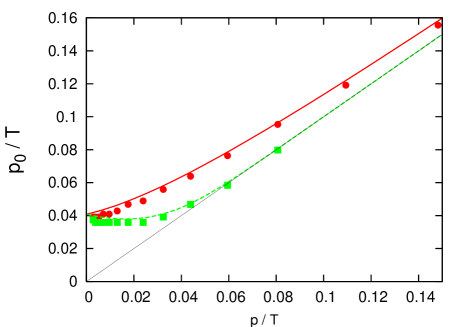
Figure 2: Peak positions of the spectral functions for the normal quasi-fermion (circles) and the plasmino (squares) for $g=0.115$. These are determined from the peak positions of the spectral function. The solid and the dashed curves represent the dispersion relations for the quasi-fermion and the plasmino in the HTL approximation, respectively. The thin solid line corresponding to $p_{0}=p$ is also shown for convenience.

We first investigate the fermion spectrum in the weak coupling region. The spectral function $\rho_{+}$ for $p=0$ and $g=0.115$ is shown in Fig. 1. We see that $\rho_{+}$ has two sharp peaks, one in the positive energy region, corresponding to the normal quasi-fermion, and the other in the negative energy region, corresponding to the anti-plasmino. The peak positions of $\rho_{+}$ and $\rho_{-}$ for positive energy and finite momentum are plotted in Fig. 2, which displays approximate dispersion relations of these excitations. We see that the dispersion relations obtained from the SDE are in good agreement with those obtained with the HTL approximation, which is valid in the weak coupling region. The narrow widths of the peaks imply that the spectra from the SDE are quite similar to those in the HTL approximation in the weak coupling region. This result is natural, because the SDE here contains the fermion self-energy in the HTL approximation, which is dominant in the weak coupling region in our approach, as expected.

Figure 3: The spectral functions $\rho_{+}$ for $g=1.15$ (left), $g=3$ (middle), and $g=6.9$ (right). The peak for $p_{0}>0~{}(<0)$ corresponds to the normal quasi-fermion (the anti-plasmino). The figure is clipped at $\rho_{+}T=0.3$.

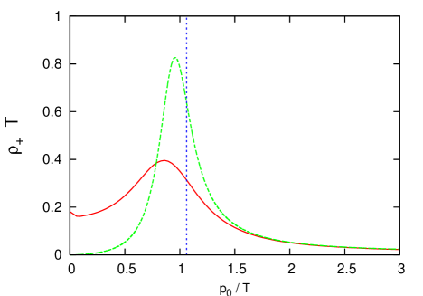
Figure 4: The spectral functions $\rho_{+}$ at rest ($p=0$) for $g=3$. The solid curve represents the spectral function obtained from the SDE, the dashed curve that from the one-loop self-energy, and the dotted line that from the HTL approximation.

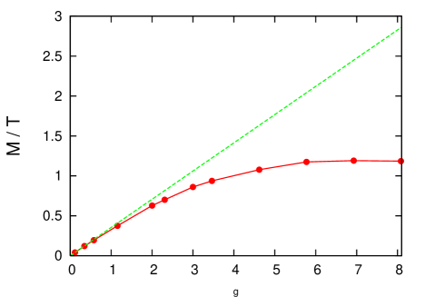
Figure 5: Coupling dependence of the thermal mass. The solid curve represents the thermal mass obtained from the SDE, and the dashed line that from the HTL approximation.

Figure 6: Cutoff dependence of the ratio $M/T$ for $g=6.9$. The solid line represents $M/T=1.19$.

For the case of strong coupling, we plot the spectral functions $\rho_{+}$ for $g=1.15,3$ and $6.9$ in Fig. 3. All the spectral functions appearing in Fig. 3 have two peaks but with broad widths. This shows that the normal quasi-fermion and the plasmino appear even in the strong coupling region. We see that as the coupling becomes larger, the widths become broader. In the case of extremely strong coupling, e.g. $g=6.9$, the peaks are so broad at low momenta that the quasi-particle picture is no longer valid. For these three couplings, we have confirmed that as the momentum becomes higher, the peak of the plasmino becomes smaller, and the peak of the normal quasi-fermion becomes larger and sharper. This behavior is due to the fact that thermal effects become smaller as the momentum increases, and thus the spectrum approaches that for the free fermion. This momentum dependence of the heights of these peaks is similar to that of the residues of the peaks in the HTL approximation.

In the left and middle panels of Fig. 3, there is another small peak at the origin in addition to the two obvious peaks. We comment on this peak in §3.2.

In Fig. 4, we plot the spectral function $\rho_{+}$ for $g=3$ and $p=0$ in the positive energy region and compare it with that obtained from the one-loop self-energy and that obtained in the HTL approximation. This figure shows that the peak obtained at one-loop order is already broad in the strong coupling region. It also shows that the peak from the SDE becomes even broader owing to non-perturbative effects. Because the SDE contains effects of multiple scatterings with gauge bosons through the self-consistency condition, the broadening of the peaks could be understood from the fact that the probability of gauge boson emission and absorption from a fermion increases rapidly with the coupling.

Now, we interpret the peak positions for $p=0$ as the thermal masses of the excitations irrespectively of the widths. In Fig. 5 we plot the coupling dependence of the thermal mass together with that obtained in the HTL approximation. We note that the thermal masses of the normal quasi-fermion and the plasmino are always the same in the chiral limit at zero density[20]. We see that in the weak coupling region, the thermal mass from the SDE almost coincides with that in the HTL approximation, and both of them are proportional to the coupling, $g$. In the strong coupling region, by contrast, the thermal mass from the SDE becomes saturated at $M\sim T$ and is almost independent of the $g$.

Before ending this subsection, we study the dependence of the resultant fermion spectrum on the choice of the ultraviolet cutoff $\Lambda$. In Fig. 6 we show the $\Lambda$-dependence of $M/T$ for $g=6.9$. We see that the ratio is almost constant, $M/T\sim 1.2$, for $\Lambda/T\gtrsim 2.5$. This implies that the thermal mass is determined by only $T$ which gives an infrared scale of the system. Furthermore, we have confirmed that the fermion spectral functions shown in Fig. 3 have little dependence on the cutoff for $p_{0}\sim M$. The shapes of the spectral function in the large $p_{0}$ region are slightly modified when we use smaller cutoff, while we see the tendency for the peak of the normal quasi-fermion becomes larger and sharper as the momentum becomes higher. Thus, we conclude that the thermal mass $M$, as well as the tendency of the shape, is not affected by cutoff artifacts for $\Lambda/T\gtrsim 2.5$. For $\Lambda/T\lesssim 2.5$, however, deviation from a constant value is seen. There cutoff effects might start to contribute.

3.2 Comment on the three-peak structure

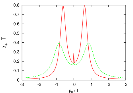
Figure 7: The spectral functions $\rho_{+}$ at rest ($p=0$) for $g=3$ (dashed curve) and $g=2$ (solid curve).

Finally, we give a comment on the peak around the origin that appears in the spectral function for $g=3$, as seen in the previous section. This peak is more pronounced for weaker coupling, $g=2$, as shown in Fig. 7. For stronger coupling, such a peak is not seen. One possible reason for this behavior is that large widths of all the peaks due to multiple scatterings with gauge bosons may conceal the peak structure around the origin.

It has been shown in Yukawa models a similar peak appears in the fermion spectral function owing to the coupling with a massive boson at finite $T$[21, 22]. In this case, the mass of the boson is essential for the formation of the three-peak structure in the fermion spectral function. In our case, however, the fermion couples to a massless gauge boson, and thus another mechanism makes it possible to form the three-peak structure. Because the SDE is a self-consistent equation for the full fermion propagator, the internal fermion in the self-energy has a thermal mass. Therefore, the system is similar to that consisting of a fermion with a thermal mass coupled to a massless gauge boson. Here, as an example of such a system, we consider an interaction of a fermion with a thermal mass obtained in the HTL approximation and a massless gauge boson at one loop. We summarize the details of this analysis in Appendix D. Figures 10 and 11 in Appendix D plot the imaginary part of the fermion self-energy and the spectral function at rest in this model. We see that the imaginary part of the self-energy possesses two peaks, which lead to the three-peak structure in the spectral function, as shown in Refs. Kitazawa:2006zi and Mitsutani:2007gf. Therefore, the existence of the three-peak structure of the spectral function from the SDE can be understood from this result.

4 Summary and discussion

We have investigated the fermion spectrum in the chiral symmetric phase employing the Schwinger-Dyson equation (SDE) for the fermion propagator with the ladder approximation and fixed gauge coupling, in which the free gauge boson propagator in the Feynman gauge is used. Because we employed the imaginary time formalism to construct the SDE, analytic continuation to the real time axis is needed to obtain the fermion spectrum. This was done by solving an integral equation for the retarded fermion propagator, following a method developed in Ref. ac. This method is known as a reliable way to carry out numerical analytic continuations in condensed matter physics, and we have confirmed in this study that it is also effective even in a relativistic system.

We have investigated the fermion spectrum in the chiral symmetric phase over a wide range of values of the gauge coupling using the method of analytic continuation mentioned above. We found that in the weak coupling region ($g\ll 1$), the fermion spectrum is quite similar to that obtained in the hard thermal loop (HTL) approximation: There exist a normal quasi-fermion and a plasmino whose thermal masses are almost the same as those found in the HTL approximation, $M\sim M_{\rm HTL}=gT/\sqrt{\mathstrut 8}$, and their widths are very narrow. (These widths vanish in the HTL approximation.) This result is natural, because the SDE here contains the HTL of the fermion self-energy, and thus the HTL is dominant in the weak coupling region in our approach, as expected.

In the strong coupling region $(g>1)$, we find that there exist a normal quasi-fermion and a plasmino, as in the weak coupling region. However, their spectra deviate from those in the HTL approximation: Both the excitation modes have smaller thermal masses and much broader widths in the low-momentum region. The thermal mass $M$ saturates at some value of the gauge coupling, and satisfies $M\sim T$ independently of the value of the coupling. Although we do not have any plausible explanation for the saturation of the thermal mass at present, the saturated value $M\sim T$ is consistent with the results of other model analyses [9, 6, 10, 8, 21]. In Ref. Mannarelli:2005pz, the broad width is described in terms of the imaginary part of the self-energy, while in our study, it is described in terms of the spectral function. Furthermore, we have shown that as the gauge coupling becomes larger, the widths rapidly become broader. This indicates that the broadening of the widths can be understood from the fact that the probability of gauge boson emission and absorption from a fermion increases rapidly with the coupling.

Our result shows that as the momentum $p$ becomes higher, the peak of the plasmino becomes smaller and the peak of the normal quasi-fermion becomes higher and sharper. Thus the spectrum approaches the free-fermion one. This behavior is similar to that in the weak coupling region and is natural because thermal effects are weaker in general for $p>T$. The free-fermion spectrum in the high momentum region is consistent with the quark recombination or coalescence picture,[23] in which the quasi-quark picture is valid.

One reason we have adopted the Feynman gauge is for the simplicity of the numerical analytic continuation mentioned above. We expect that the qualitative features of the fermion spectrum discussed in this paper do not change even if we adopt other gauge fixings.

We now discuss what our result can provide regarding the quark spectrum in the real-life QCD at high temperature. In the very high temperature region of QCD, the HTL approximation is valid for studying the quark spectrum. In the HTL approximation, the fixed coupling, which is the running coupling at an energy scale of order $T$, say $g(T)$, is used, because the quarks and gluons with energy $T$ give the dominant contribution. In studying the quark spectrum in the lower $T$ region, the diagrams other than the HTL start to give non-negligible corrections, since the (fixed) coupling $g(T)$ is larger. For this reason, we can state that, in our approach, we include a part of the corrections from all the ladder diagrams by solving the Schwinger-Dyson equation. Actually, our result reproduces that of the HTL approximation in the weak coupling region, i.e. in the very high temperature region where $g(T)$ is small. In the lower temperature region, where $g(T)$ is large, our result in the strong coupling region suggests that the corrections from the ladder diagrams have the following effects on the qualitative structure of the quark spectrum: (1) The thermal masses of quark and plasmino are not proportional to the gauge coupling $g(T)$, becoming $M\sim T$, and (2) their widths are very broad, due to multiple scatterings with gluons.

In this study, we have used the free gauge boson propagator in the SDE. In medium, however, the gauge boson spectrum may also change significantly, as in the HTL approximation. One possible extension to include such an effect is to use the gauge boson propagator with Debye screening and a dynamical screening that has the same form as that in the HTL approximation. Such a study is left as a future project.

Appendix A Notation

Here, we briefly give definitions of some of the quantities used in this paper.

The Matsubara Green function is defined by

$$\mathcal{S}(i\omega_{n},\vec{p})\equiv{\rm F.T.}\langle T_{\tau}\psi(\tau,\vec{r})\overline{\psi}(\tau^{\prime},\vec{r^{\prime}})\rangle_{T}\,\,,$$ (19)

where $\langle\cdots\rangle_{T}$ stands for the thermal average with temperature $T$. The retarded Green function for a fermion $S_{R}$ and the spectral function for a fermion are defined by

$$S_{R}(t,\vec{r};t^{\prime},r^{\prime})\equiv\theta(t-t^{\prime})\langle\{\psi(t,\vec{r}),\overline{\psi}(t^{\prime},\vec{r^{\prime}})\}\rangle_{T}\,\,,$$ (20)

$$\rho(p_{0},p)=\frac{1}{2\pi}{\rm F.T.}\langle\{\psi(t,\vec{r}),\overline{\psi}(t^{\prime},\vec{r^{\prime}})\}\rangle_{T}\,\,.$$ (21)

The retarded Green function and the Matsubara Green function are related to the spectral function by the spectral representations as

$$\mathcal{S}(i\omega_{n},\vec{p}) =-\int_{-\infty}^{\infty}dp_{0}^{\prime}\frac{\rho(p_{0}^{\prime},\vec{p})}{i\omega_{n}-p_{0}^{\prime}}\,\,,$$ (22)

$$iS_{R}(p_{0},\vec{p}) =-\int_{-\infty}^{\infty}dp_{0}^{\prime}\frac{\rho(p_{0}^{\prime},\vec{p})}{p_{0}-p_{0}^{\prime}+i\epsilon}\,\,.\$$ (23)

These functions for gauge bosons can be written in the same forms.

Appendix B Phase Structure

Figure 8: Temperature dependence of the function $B(i\omega_{n}=0,p=0)/\Lambda$ (left) and the effective potential $V_{\rm rel}(T)/\Lambda^{4}$ (right) for $g=6.9$.

In this appendix, we compute the critical temperature $T_{c}$ to specify the chiral symmetric phase. We introduce the effective potential for the fermion propagator to determine the phase structure and $T_{c}$,[18]

$$V(\mathcal{S}) =T\sum_{n=-\infty}^{\infty}\int\frac{d^{3}\vec{p}}{(2\pi^{3})}\{\ln\det[\mathcal{S}(i\omega_{n},\vec{p})]+{\rm tr}[\ooalign{\hfil/\hfil\crcr$p$}\mathcal{S}(i\omega_{n},\vec{p})]\}$$ (26)

$$+\frac{1}{2}g^{2}T^{2}\sum_{n,m=-\infty}^{\infty}\int\frac{d^{3}\vec{p}}{(2\pi)^{3}}\int\frac{d^{3}\vec{k}}{(2\pi)^{3}}$$

$$\hskip 20.00003pt\times{\rm tr}\left[\mathcal{S}(i\omega_{n},\vec{p})\gamma_{\mu}\mathcal{S}(i\omega_{m},\vec{k})\gamma_{\nu}\right]\mathcal{D}^{\mu\nu}(i\omega_{n}-i\omega_{m},\vec{p}-\vec{k})\,\,,$$ (27)

where ${\rm ln}$, $\det$ and ${\rm tr}$ are taken in the spinor spaces. The SDE is obtained as the stationary condition for the effective potential (27). Note that the value of the potential is meaningful only at the stationary point; i.e. the potential can be evaluated only when the solution of the SDE is substituted. There always exists a solution of the SDE with $B=0$. In the low temperature region, we also have a solution with $B\neq 0$, which corresponds to dynamical chiral symmetry breaking. Let $\mathcal{S}_{W}$ denote the solution with $B=0$ and $\mathcal{S}_{NG}$ the solution with $B\neq 0$. They are parameterized as

$$[\mathcal{S}_{W}(i\omega_{n},\vec{p})]^{-1} \equiv A_{W}(i\omega_{n},p)\vec{p}\cdot\vec{\gamma}-C_{W}(i\omega_{n},p)i\omega_{n}\gamma_{0}\,\,,$$ (28)

$$[\mathcal{S}_{NG}(i\omega_{n},\vec{p})]^{-1} \equiv B_{NG}(i\omega_{n},p)+A_{NG}(i\omega_{n},p)\vec{p}\cdot\vec{\gamma}-C_{NG}(i\omega_{n},p)i\omega_{n}\gamma_{0}\,\,.$$ (29)

To determine which of the solutions $\mathcal{S}_{W}$ and $\mathcal{S}_{NG}$ gives the real vacuum, we compare the values of the effective potential with each solution by computing the following difference:

$$V_{\rm rel}(T) \equiv V(\mathcal{S}_{NG})-V(\mathcal{S}_{W})$$

$$=-\frac{1}{\pi^{2}}T\sum_{m=-\infty}^{\infty}\int_{0}^{\Lambda}dpp^{2}\Biggl{\{}\ln\left[\frac{p^{2}A_{NG}^{2}(i\omega_{n},p)+\omega_{n}^{2}C_{NG}^{2}(i\omega_{n},p)+B_{NG}^{2}(i\omega_{n},p)}{p^{2}A_{W}^{2}(i\omega_{n},p)+\omega_{n}^{2}C_{W}^{2}(i\omega_{n},p)}\right]$$

$$\ +\frac{p^{2}A_{NG}(i\omega_{n},p)+\omega_{n}^{2}C_{NG}(i\omega_{n},p)}{p^{2}A_{NG}^{2}(i\omega_{n},p)+\omega_{n}^{2}C_{NG}^{2}(i\omega_{n},p)+B_{NG}^{2}(i\omega_{n},p)}$$

$$\ -\frac{p^{2}A_{W}(i\omega_{n},p)+\omega_{n}^{2}C_{W}(i\omega_{n},p)}{p^{2}A_{W}^{2}(i\omega_{n},p)+\omega_{n}^{2}C_{W}^{2}(i\omega_{n},p)}\Biggr{\}}\,\,.\,\,$$ (30)

For $V_{\rm rel}(T)<0$, the chiral broken vacuum is realized, while the chiral symmetric phase becomes the true vacuum for $V_{\rm rel}(T)\geq 0$. We determine $T_{c}$ as the smallest value of $T$ at which $V_{\rm rel}(T)$ vanishes.

Figure 9: Coupling dependence of the critical temperature $T_{c}/\Lambda$. The chiral symmetric (broken) phase is above (below) the line.

We plot the $T$ dependence of the function $B(i\omega_{n},p)$ for the smallest Matsubara frequency at $p=0$ in the left panel and that of the potential $V_{\rm rel}$ in the right panel of Fig. 8. It is seen that the function $B$ and the potential $V_{\rm rel}$ simultaneously go to zero smoothly with $T$. This implies that the chiral phase transition is of second order. The value of the critical temperature is determined as $T_{c}/\Lambda\simeq 0.18$ for $g=6.9$. The value $T_{c}/\Lambda$ depends on the coupling. In Fig. 9, we plot $T_{c}/\Lambda$ for each coupling. Note that the chiral broken vacuum is not realized even at $T=0$ for $g<g_{c}\simeq 5.1$.

Appendix C Analytic Continuation for Solutions
of the Schwinger-Dyson Equation

In this appendix, we explain the details of the method for the analytic continuation used in the present analysis, following Ref. ac.

Let us start with the spectral representations for the fermion and gauge boson propagators,

$$\mathcal{S}(i\omega_{m},\vec{k}) =-\int_{-\infty}^{\infty}dz\frac{\rho_{F}(z,\vec{k})}{i\omega_{m}-z}=-\frac{1}{\pi}\int_{-\infty}^{\infty}dz\frac{{\rm Im}iS_{R}(z,\vec{k})}{i\omega_{m}-z}\,\,,$$ (31)

$$\mathcal{D}_{\mu\nu}(i\omega_{n}-i\omega_{m},\vec{p}-\vec{k}) =-\int_{-\infty}^{\infty}dz\frac{\rho_{B}^{\mu\nu}(z,\vec{p}-\vec{k})}{(i\omega_{n}-i\omega_{m})-z}\,\,,$$ (32)

where $\rho_{F}$ and $\rho_{B}^{\mu\nu}$ represent the spectral functions of fermion and the gauge boson, respectively. The function $S_{R}(z,\vec{k})$ is the retarded fermion propagator, which is analytic in the upper half complex plane of the variable $z$.

Using the above spectral representations, the summation over the Matsubara frequencies in the SDE (3) is performed by replacing the sums over frequencies with the following contour integral:

$$T\sum_{m=-\infty}^{\infty}f(k_{0}=i\omega_{m})=\oint_{c}\frac{dk_{0}}{2\pi i}f(k_{0})\frac{1}{2}{\rm tanh}\frac{k_{0}}{2T}\,\,.$$ (33)

Then we replace the Matsubara frequency as $i\omega_{n}\rightarrow p_{0}+i\epsilon$. Thus we obtain the SDE for the retarded fermion propagator as follows:

$$iS_{R}^{-1}(p_{0},\vec{p})-iS_{R\,\,{\rm{free}}}^{-1}(p_{0},\vec{p})$$

$$=-\frac{g^{2}}{\pi}\int\frac{d^{3}k}{(2\pi)^{3}}\int_{-\infty}^{\infty}dz\int_{-\infty}^{\infty}dz^{\prime}$$

$$\ \times\Biggl{[}\gamma_{\mu}\frac{{\rm Im}[iS_{R}(z,\vec{k})]}{p_{0}-z-z^{\prime}+i\epsilon}\gamma_{\nu}\rho_{B}^{\mu\nu}(z^{\prime},\vec{p}-\vec{k})\frac{1}{2}\left(\tanh\frac{z}{2T}+\coth\frac{z^{\prime}}{2T}\right)\Biggr{]}\,\,.$$ (34)

By using the relations ${\rm Re}[f(z)]={\rm Im}[if(z)]$ and ${\rm Im}[f(z)]={\rm Re}[-if(z)]$, Eq. (34) can be rewritten as

$$iS_{R}^{-1}(p_{0},\vec{p})-iS_{R\,\,{\rm{free}}}^{-1}(p_{0},\vec{p})$$

$$=-\frac{g^{2}}{4\pi}\int_{-\infty}^{\infty}dz^{\prime}\int\frac{d^{3}\vec{k}}{(2\pi)^{3}}\rho_{B}^{\mu\nu}(z^{\prime},\vec{p}-\vec{k})\gamma_{\mu}$$

$$\hskip 10.00002pt\times\Biggl{\{}{\rm Im}\Biggl{[}\int_{-\infty}^{\infty}dziS_{R}(z,\vec{k})\left(\frac{1}{p_{0}-z-z^{\prime}+i\epsilon}+\frac{1}{p_{0}-z-z^{\prime}-i\epsilon}\right)$$

$$\hskip 30.00005pt\times\left({\rm tanh}\frac{z}{2T}+{\rm coth}\frac{z^{\prime}}{2T}\right)\Biggr{]}$$

$$\hskip 30.00005pt-i{\rm Re}\Biggl{[}\int_{-\infty}^{\infty}dziS_{R}(z,\vec{k})\left(\frac{1}{p_{0}-z-z^{\prime}+i\epsilon}-\frac{1}{p_{0}-z-z^{\prime}-i\epsilon}\right)$$

$$\hskip 30.00005pt\times\left({\rm tanh}\frac{z}{2T}+{\rm coth}\frac{z^{\prime}}{2T}\right)\Biggr{]}\Biggr{\}}\gamma_{\nu}\,\,.$$ (35)

Because the retarded fermion propagator, $S_{R}$, should be analytic in the upper half complex $z$ plane, the integrand of the right-hand side can have poles only at $z=p_{0}-z^{\prime}+i\epsilon$ and $z=i(2n+1)\pi T$ for $n\geq 0$. Then, the integration over $z$ can be replaced by the contour integral. Then, performing the contour integral over $z$, we obtain

$$iS_{R}^{-1}(p_{0},\vec{p})-iS_{R\,\,{\rm{free}}}^{-1}(p_{0},\vec{p})$$

$$=-\frac{g^{2}}{2\pi}\int_{-\infty}^{\infty}dz^{\prime}\int\frac{d^{3}\vec{k}}{(2\pi)^{3}}\rho_{B}^{\mu\nu}(z^{\prime},\vec{p}-\vec{k})\gamma_{\mu}$$

$$\hskip 10.00002pt\times\Biggl{\{}{\rm Im}\Biggl{[}2i\pi T\sum_{m=0}^{\infty}iS_{R}(i\omega_{m},\vec{k})\left(\frac{1}{p_{0}-i\omega_{m}-z^{\prime}+i\epsilon}+\frac{1}{p_{0}-i\omega_{m}-z^{\prime}-i\epsilon}\right)$$

$$\hskip 50.00008pt-i\pi iS_{R}(p_{0}-z^{\prime},\vec{k})\left({\rm tanh}\frac{p_{0}-z^{\prime}}{2T}+{\rm coth}\frac{z^{\prime}}{2T}\right)\Biggr{]}$$

$$\hskip 30.00005pt-i{\rm Re}\Biggl{[}2i\pi T\sum_{m=0}^{\infty}iS_{R}(i\omega_{m},\vec{k})\left(\frac{1}{p_{0}-i\omega_{m}-z^{\prime}+i\epsilon}-\frac{1}{p_{0}-i\omega_{m}-z^{\prime}-i\epsilon}\right)$$

$$\hskip 60.00009pt-i\pi iS_{R}(p_{0}-z^{\prime},\vec{k})\left({\rm tanh}\frac{p_{0}-z^{\prime}}{2T}+{\rm coth}\frac{z^{\prime}}{2T}\right)\Biggr{]}\Biggr{\}}\gamma_{\nu}\,\,.$$ (36)

In the above expression, we can drop the term $i\epsilon$, because the Matsubara frequency, $\omega_{m}$, is always non-zero. Using the relations ${\rm Im}f(z)-i{\rm Re}f(z)=-if(z)$ and ${\rm Im}f(z)+i{\rm Re}f(z)=if(z)^{*}$, we obtain

$$iS_{R}^{-1}(p_{0},\vec{p})-iS_{R\,\,{\rm{free}}}^{-1}(p_{0},\vec{p})$$

$$=-g^{2}\int_{-\infty}^{\infty}dz^{\prime}\int\frac{d^{3}\vec{k}}{(2\pi)^{3}}\rho_{B}^{\mu\nu}(z^{\prime},\vec{p}-\vec{k})\gamma_{\mu}\Biggl{[}T\sum_{m=0}^{\infty}\left(\frac{S(i\omega_{m},\vec{k})}{p_{0}-i\omega_{m}-z^{\prime}}+\frac{S^{*}(i\omega_{m},\vec{k})}{p_{0}-i\omega_{m}-z^{\prime}}\right)$$

$$\ -iS_{R}(p_{0}-z^{\prime},\vec{k})\frac{1}{2}\left({\rm tanh}\frac{p_{0}-z^{\prime}}{2T}+{\rm coth}\frac{z^{\prime}}{2T}\right)\Biggr{]}\gamma_{\nu}\,\,.$$ (37)

Finally, because the Matsubara Green function is real, i.e. $S(i\omega_{m},\vec{k})=S(i\omega_{m},\vec{k})^{*}$, we arrive at

$$iS_{R}^{-1}(p_{0},\vec{p})-iS_{R\,\,{\rm free}}^{-1}(p_{0},\vec{p})$$

$$=-g^{2}\int\frac{d^{3}\vec{k}}{(2\pi)^{3}}\int_{-\infty}^{\infty}dzT\sum_{m=-\infty}^{\infty}\gamma_{\mu}\left[\frac{\mathcal{S}(i\omega_{m},\vec{k})}{p_{0}-z-i\omega_{m}}\right]\gamma_{\nu}\rho_{B}^{\mu\nu}(z,\vec{p}-\vec{k})$$

$$\hskip 10.00002pt+g^{2}\int\frac{d^{3}\vec{k}}{(2\pi)^{3}}\int_{-\infty}^{\infty}dz\gamma_{\mu}iS_{R}(p_{0}-z,\vec{k})\gamma_{\nu}\rho_{B}^{\mu\nu}(z,\vec{p}-\vec{k})\frac{1}{2}\left[{\rm tanh}\frac{p_{0}-z}{2T}+{\rm coth}\frac{z}{2T}\right]\,\,.$$ (38)

With the solution of Eq. (3) substituted into ${\mathcal{S}}(i\omega_{m},\vec{k})$, Eq. (38) becomes a self-consistent equation for the retarded fermion propagator. In this way, we can perform the analytic continuation for the solution of the SDE by solving the integral equation (38).

Note that the first term in Eq. (38) is obtained through the naive replacement $i\omega_{n}\rightarrow p_{0}+i\epsilon$ in Eq. (3), which is easily checked by integrating over $z$ in Eq. (38). The second term appears from the fact that the Matsubara summation must be done before the analytic continuation. We can also verify that Eq. (38) returns to the original SDE (3) through the replacement $p_{0}\rightarrow i\omega_{n}$.

Appendix D Three-Peak Structure in a Simple Model

In this appendix, we show that the three-peak structure of the fermion spectrum obtained in the SDE can be understood from the interaction of a fermion with a thermal mass and a free gauge boson. For simplicity, let us consider a one-loop diagram consisting of a fermion propagator obtained in the HTL approximation and a massless gauge boson propagator. Then, the fermion self-energy is given by

$$\Sigma(i\omega_{n},\vec{p})=-g^{2}T\sum\int\frac{d^{3}k}{(2\pi)^{3}}\gamma_{\mu}{\mathcal{S}}^{\rm HTL}(i\omega_{m},\vec{k})\gamma_{\nu}{\mathcal{D}}^{\mu\nu}_{\rm free}(i\omega_{n}-i\omega_{m},\vec{p}-\vec{k})\,\,,$$ (39)

where ${\mathcal{S}}^{\rm HTL}$ is the fermion propagator obtained in the HTL approximation and ${\mathcal{D}}_{\rm free}^{\mu\nu}$ is the free gauge boson propagator in the Feynman gauge. The retarded fermion propagator in the HTL approximation is decomposed as

$$-iS_{R}^{\rm HTL}(p_{0},\vec{p})=\frac{\frac{1}{2}(\gamma_{0}-\vec{\gamma}\cdot\hat{\vec{p}})}{D_{+}^{\rm HTL}(p_{0},\vec{p})}+\frac{\frac{1}{2}(\gamma_{0}+\vec{\gamma}\cdot\hat{\vec{p}})}{D_{-}^{\rm HTL}(p_{0},\vec{p})}\,\,,$$ (40)

where $D_{+}^{\rm HTL}$ is for the fermion and $D_{-}^{\rm HTL}$ for the anti-fermion. The quantities $D_{\pm}^{\rm HTL}$ are related to the spectral function $\rho_{\pm}^{\rm HTL}$ as in Eq. (18). The spectral functions $\rho_{\pm}^{\rm HTL}$ can be written as

$$\rho^{\rm HTL}_{\pm}(p_{0},p)=Z_{\pm}(p)\delta(p_{0}-\omega_{\pm}(p))+Z_{\mp}(p)\delta(p_{0}+\omega_{\mp}(p))+\rho_{\pm}^{c}(p_{0},p)\,\,,$$ (41)

where $Z_{\pm}(k)=(\omega_{\pm}^{2}(k)-k^{2})/2M_{\rm HTL}^{2}$ are pole residues, with $M_{\rm HTL}^{2}=g^{2}T^{2}/8$, and $\rho_{\pm}^{c}$ are the continuum parts, given by

$$\rho^{c}_{\pm}(p_{0},p) =\frac{1}{2p}M_{\rm HTL}^{2}(1\mp x)\theta(1-x^{2})$$

$$\times\left[(p(1\mp x)\pm\frac{M_{\rm HTL}^{2}}{2p}[(1\mp x)\ln\left|\frac{x+1}{x-1}\right|\pm 2])^{2}+\frac{\pi^{2}M_{\rm HTL}^{4}}{4p^{2}}(1\mp x)^{2}\right]^{-1}\,\,,$$ (42)

with $x=p_{0}/p$. In the following, we limit ourselves to the rest frame ($p=0$). Using $\rho_{\pm}^{\rm HTL}$, we obtain

$$\Sigma_{0}(i\omega_{n},0) =\frac{1}{4}{\rm tr}[\gamma_{0}\Sigma(i\omega_{n},0)]$$

$$=-g^{2}T\sum\int\frac{d^{3}k}{(2\pi)^{3}}\int dz\frac{\rho^{\rm HTL}_{+}(z,{k})+\rho^{\rm HTL}_{-}(z,{k})}{i\omega_{m}-z}\int dz^{\prime}\frac{\rho_{B}(z^{\prime},{k})}{i\omega_{n}-i\omega_{m}-z^{\prime}}\,\,,$$ (43)

with $\rho_{B}(p_{0},p)=\epsilon(p_{0})\delta(p_{0}^{2}-p^{2})$. By carrying out the Matsubara summation and the replacement $i\omega_{n}\rightarrow p_{0}+i\epsilon$, $\Sigma_{0}$ becomes

$$\Sigma_{0}(p_{0},0) =g^{2}\int\frac{d^{3}k}{(2\pi)^{3}}\int dz\int dz^{\prime}\frac{1-f(z)+n(z^{\prime})}{p_{0}-z-z^{\prime}+i\epsilon}$$

$$\ \times\left[\rho^{\rm HTL}_{+}(z,{k})+\rho^{\rm HTL}_{-}(z,{k})\right]\rho_{B}(z^{\prime},{k})\,\,,$$ (44)

with $f(E)=[\exp(E/T)+1]^{-1}$ and $n(E)=[\exp(E/T)-1]^{-1}$. The imaginary part of $\Sigma_{0}$ can be easily calculated as

$${\rm Im}\Sigma_{0} =\frac{g^{2}}{4\pi}\Biggl{[}\frac{kZ_{+}(k)}{|1+\omega_{+}^{\prime}|}(f(p_{0}-k)-n(k)-1)\Big{|}_{p_{0}-k-\omega_{+}(k)=0}$$

$$\ +\frac{kZ_{-}(k)}{|1-\omega_{-}^{\prime}|}(f(p_{0}-k)-n(k)-1)\Big{|}_{p_{0}-k+\omega_{-}(k)=0}$$

$$\ +\frac{kZ_{-}(k)}{|1+\omega_{-}^{\prime}|}(f(p_{0}-k)-n(k)-1)\Big{|}_{p_{0}-k-\omega_{-}(k)=0}$$

$$\ +\frac{kZ_{+}(k)}{|1-\omega_{+}^{\prime}|}(f(p_{0}-k)-n(k)-1)\Big{|}_{p_{0}-k+\omega_{+}(k)=0}$$

$$\ -\frac{kZ_{+}(k)}{|1-\omega_{+}^{\prime}|}(f(p_{0}+k)+n(k))\Big{|}_{p_{0}+k-\omega_{+}(k)=0}$$

$$\ -\frac{kZ_{-}(k)}{|1+\omega_{-}^{\prime}|}(f(p_{0}+k)+n(k))\Big{|}_{p_{0}+k+\omega_{-}(k)=0}$$

$$\ -\frac{kZ_{-}(k)}{|1-\omega_{-}^{\prime}|}(f(p_{0}+k)+n(k))\Big{|}_{p_{0}+k-\omega_{-}(k)=0}$$

$$\ -\frac{kZ_{+}(k)}{|1+\omega_{+}^{\prime}|}(f(p_{0}+k)+n(k))\Big{|}_{p_{0}+k+\omega_{+}(k)=0}\Biggr{]}$$

$$\ +\frac{g^{2}}{4\pi}\int dkk\Bigl{[}(f(p_{0}-k)-n(k)-1)(\rho_{+}^{c}(p_{0}-k,k)+\rho_{-}^{c}(p_{0}-k,k))$$

$$\hskip 70.0pt-(f(p_{0}+k)+n(k))(\rho_{+}^{c}(p_{0}+k,k)+\rho_{-}^{c}(p_{0}+k,k))\Bigr{]}\,\,,$$ (45)

with $\omega_{\pm}^{\prime}=d\omega_{\pm}(k)/dk$.

It is noted that Eq. (45) is divergence-free. The real part of $\Sigma_{0}$, by contrast, has an ultraviolet divergence, and here we regularize it using the relation

$${\rm Re}\Sigma_{0}(p_{0},0)=-\frac{1}{\pi}{\rm P}\int_{-\Lambda}^{\Lambda}dp_{0}^{\prime}\frac{{\rm Im}\Sigma_{0}(p_{0}^{\prime},0)}{p_{0}-p_{0}^{\prime}}\,\,,$$ (46)

with the three-momentum cutoff $\Lambda$. We choose $\Lambda$ to satisfy $T/\Lambda=0.3$. Here, ${\rm P}$ represents the principal-value operator. By using $\Sigma_{0}$, the spectral function at rest is obtained as

$$\rho_{\pm}(p_{0},0)=-\frac{1}{\pi}{\rm Im}\frac{1}{p_{0}-\Sigma_{0}(p_{0},0)}\,\,.$$ (47)

Figure 10: The imaginary part of the self-energy for $g=2$, $T/\Lambda=0.3$ at rest ($p=0$).

Figure 11: The spectral function for $g=2$, $T/\Lambda=0.3$ at rest ($p=0$).

Now, we present our numerical result for $g=2$. In Fig. 10 we plot the $p_{0}$ dependence of the imaginary part of the self-energy, ${\rm Im}\Sigma_{0}(p_{0},0)$. We see two distinct peaks for $|p_{0}/M_{\rm HTL}|<1$, which come from the Landau damping and the kinematics: The Landau damping implies a non-vanishing imaginary part that is even for $|p_{0}/M_{\rm HTL}|<1$, while the imaginary part vanishes at the origin, because of the suppression of the decay rate for distribution functions. These two peaks in ${\rm Im}\Sigma_{0}(p_{0},0)$ are similar to those in the system studied in Ref. Kitazawa:2006zi with a massless fermion and a massive boson that result from a Yukawa coupling. Because the current fermion mass is taken to be zero, the fermion spectrum is determined solely from the structure of the imaginary part of the self-energy, as shown in Eq. (47). Therefore, the fermion spectrum should also be similar to that obtained in Refs. Kitazawa:2006zi and Mitsutani:2007gf, and actually form a three-peak structure, as shown in Fig. 11, which is qualitatively the same as that in Refs. Kitazawa:2006zi and Mitsutani:2007gf.

The peak around the origin in Fig. 11 is very sharp, because the imaginary part of the self-energy vanishes at the origin, as mentioned above. Contrastingly, the peak at the origin obtained using the SDE is not so sharp, due to the non-perturbative iteration: If we use the spectral function (47) for the internal fermion line in Eq. (39) instead of ${\mathcal{S}}_{\rm HTL}$ as an effect of the iteration, the imaginary part of the resultant self-energy will be non-zero even at the origin, and the peak around the origin should become broader.

References

• [1] I. Arsene et al., Nucl. Phys. A 757 (2005), 1. B. B. Back et al., Nucl. Phys. A 757 (2005), 28. J. Adams et al., Nucl. Phys. A 757 (2005), 102. K. Adcox et al., Nucl. Phys. A 757 (2005), 184.
• [2] M. Asakawa and T. Hatsuda, Phys. Rev. Lett.  92 (2004), 012001. S. Datta, F. Karsch, P. Petreczky and I. Wetzorke, Phys. Rev. D 69 (2004), 094507. T. Umeda, K. Nomura and H. Matsufuru, Eur. Phys. J. C 39S1 (2005), 9. H. Iida, T. Doi, N. Ishii, H. Suganuma and K. Tsumura, Phys. Rev.  D 74 (2006), 074502. A. Jakovac, P. Petreczky, K. Petrov and A. Velytsky, Phys. Rev.  D 75 (2007), 014506. G. Aarts, C. Allton, M. B. Oktay, M. Peardon and J. I. Skullerud, Phys. Rev.  D 76 (2007), 094513
• [3] T. Hatsuda and T. Kunihiro, Phys. Lett. B 145 (1984), 7; Phys. Rev. Lett.  55 (1985), 158. See also C. DeTar, Phys. Rev. D 32 (1985), 276.
• [4] E. V. Shuryak and I. Zahed, Phys. Rev. C 70 (2004), 021901; Phys. Rev. D 70 (2004), 054507.
• [5] G. E. Brown, C. H. Lee, M. Rho and E. Shuryak, Nucl. Phys.  A 740 (2004), 171; J. Phys. G 30 (2004), S1275. H. J. Park, C. H. Lee and G. E. Brown, Nucl. Phys.  A 763 (2005), 197. G. E. Brown, B. A. Gelman and M. Rho, Phys. Rev. Lett.  96 (2006), 132301. G. E. Brown, C. H. Lee and M. Rho, arXiv:nucl-th/0507011.
• [6] A. Schaefer and M. H. Thoma, Phys. Lett. B 451 (1999), 195. A. Peshier and M. H. Thoma, Phys. Rev. Lett.  84 (2000), 841.
• [7] P. Petreczky, F. Karsch, E. Laermann, S. Stickan and I. Wetzorke, Nucl. Phys. Proc. Suppl.  106 (2002), 513.
• [8] F. Karsch and M. Kitazawa, Phys. Lett.  B 658 (2007), 45
• [9] M. Mannarelli and R. Rapp, Phys. Rev. C 72 (2005), 064905.
• [10] M. Kitazawa, T. Kunihiro and Y. Nemoto, Phys. Lett. B 633 (2006), 269.
• [11] See, e.g., T. Kugo, in Proc. of 1991 Nagoya Spring School on Dynamical Symmetry Breaking, Nakatsugawa, Japan, 1991, ed. K. Yamawaki (World Scientific, Singapore, 1992). V. A. Miransky, Dynamical symmetry breaking in quantum field theories (Singapore, Singapore: World Scientific, 1993).
• [12] See, e.g., M. Harada and A. Shibata, Phys. Rev.  D 59 (1999), 014010; C. D. Roberts and S. M. Schmidt, Prog. Part. Nucl. Phys.  45 (2000), S1. S. Takagi, Prog. Theor. Phys.  109 (2003), 233.
• [13] T. Ikeda, Prog. Theor. Phys.  107 (2002), 403. Y. Fueki, H. Nakkagawa, H. Yokota and K. Yoshida, Prog. Theor. Phys.  110 (2003), 777.
• [14] V. V. Klimov, Sov. J. Nucl. Phys.  33 (1981), 934; Yadern. Fiz.  33 (1981), 1734. H. A. Weldon, Phys. Rev.  D 40 (1989), 2410.
• [15] F. Marsiglio, M. Schossmann and J. P. Carbotte, Phys. Rev. B 37 (1988), 4965.
• [16] H. Georgi, E. H. Simmons and A. G. Cohen, Phys. Lett. B 236 (1990), 183.
• [17] H. Nakkagawa, H. Yokota and K. Yoshida, hep-ph/0703134. H. Nakkagawa, H. Yokota and K. Yoshida, arXiv:0707.0929.
• [18] J. M. Cornwall, R. Jackiw and E. Tomboulis, Phys. Rev.  D 10 (1974), 2428.
• [19] A. Peshier, K. Schertler and M. H. Thoma, Ann. of Phys.  266 (1998), 162.
• [20] H. A. Weldon, Phys. Rev.  D 61 (2000), 036003.
• [21] M. Kitazawa, T. Kunihiro and Y. Nemoto, Prog. Theor. Phys.  117 (2007), 103.
• [22] M. Kitazawa, T. Kunihiro, K. Mitsutani and Y. Nemoto, arXiv:0710.5809.
• [23] R. J. Fries, B. Muller, C. Nonaka and S. A. Bass, Phys. Rev. Lett.  90 (2003), 202303; Phys. Rev.  C 68 (2003), 044902. V. Greco, C. M. Ko and P. Levai, Phys. Rev. Lett.  90 (2003), 202302. D. Molnar and S. A. Voloshin, Phys. Rev. Lett.  91 (2003), 092301.