Electron-electron Relaxation in Disordered Interacting Systems

Abstract

We study the relaxation of a non-equilibrium carrier distribution under the influence of the electron-electron interaction in the presence of disorder.

Based on the Anderson model, our Hamiltonian is composed from a single particle part including the disorder and a two-particle part accounting for the Coulomb interaction. We apply the equation-of-motion approach for the density matrix, which provides a fully microscopic description of the relaxation. Our results show that the nonequlibrium distribution in this closed and internally interacting system relaxes exponentially fast during the initial dynamics. This fast relaxation can be described by a phenomenological damping rate. The total single particle energy decreases in the redistribution process, keeping the total energy of the system fixed. It turns out that the relaxation rate decreases with increasing disorder.

1 Introduction

Understanding the interplay of disorder and interaction constitutes a challenging problem in condensed matter physics [1]. Even weak interactions cause a considerable amount of complexity [2]. One of the most intriguing phenomena, the phase relaxation due to interaction, has already been treated in the presence of disorder [3]. In many cases, however, either of the two major ingredients, the disorder and the inter-particle interaction are taken into account only perturbatively. In numerical simulations this type of approximation is not necessary. However, finite-size limitations do affect the results, even though further controlled simplifications may nevertheless be necessary to impose.

In this paper we present a case study where we have investigated how the interplay of disorder and long-range interaction affects the relaxation of a non-equilibrium energy distribution of electrons in one dimension.

In this paper our aims are twofold. On the one hand, we want to determine whether the relaxation within a closed interacting system can be described by a phenomenological damping rate. On the other hand, we perform the first steps in the direction of constructing a theory of relaxation treating both disorder and interaction on an equal microscopic footing. Our approach is based on the equation of motion technique applied on elements of the density matrix. This technique has achieved a great success in numerous applications in semiconductor optics for systems with strong many-body correlations [4, 5]. Our experience shows that the interplay of disorder and interaction does yield novel and interesting phenomena [6, 7]. Here we provide one more evidence that it can also be used to tackle challenging problems in the field of interacting disordered systems.

The phase relaxation due to inter-particle interactions in disordered systems has already been investigated analytically, for a recent review, see [3]. As a summary, the presence of weak disorder accelerates the relaxation process, since the scattering probabilities increase due to the lack of momentum selection rules an ordered system would impose. The question of strong disorder, however, is not yet fully understood. A first step using numerical simulations was performed in [8], where a Boltzmann-type equation was solved with an initial condition of a non-equilibrium carrier distribution, which relaxes over the course of time towards a Fermi-Dirac-type distribution. While the analytical prediction for weak disorder was recovered in the case when short-ranged interactions were allowed between the particles, for both long ranged and short ranged interaction the strong disorder limit yielded a decrease in the relaxation rate. The latter behavior was attributed to the small size of the localization volume of the one particle-states, resulting in smaller scattering probabilities.

Since the previous work of I. Varga et al. [8] suffered from several simplifying assumptions, in the present work we perform computations along similar ideas, but using a much better founded formalism, namely the equation of motion of the density matrix [5, 6, 7].

2 Model

2.1 The Hamiltonian

Our model is based on a one dimensional tight–binding model with energetic disorder, represented by the energies of the sites denoted by $\varepsilon_{j}$ for the $j^{\mathrm{th}}$ site [5, 7]. The model also includes nearest neighbor hopping matrix elements $J_{ij}=J$ between sites $i$ and $j$. Using a site basis where $\left|i\right>$ denotes the basis function at site $i$ it is straightforward to formulate the non-interacting part of the Hamiltonian:

$$H_{0}=\sum_{i}\varepsilon_{i}\left|i\right>\left<i\right|+\sum_{<ij>}J_{ij}\left|i\right>\left<j\right|\,,$$ (1)

where $<ij>$ corresponds to a sum limited to the nearest neighbors.

The term responsible for the two-body interaction reads [5]

$$\\ \\ H_{\mathrm{C}}=\frac{1}{2}\sum_{i,j}V_{ij}\,\left|i\right>\left|j\right>\left<j\right|\left<i\right|\,,\\$$ (2)

where only monopole–monopole terms have been included. In Eq. (2), the sum represents the repulsive Coulomb interaction among charge carriers within a single band. The regularized Coulomb matrix element considered here is given by

$$V_{ij}=\frac{U_{0}}{|i-j|a+a_{0}},$$ (3)

with a positive constant $U_{0}$. Here $a=5$ nm is the site separation [5] and the term $a_{0}=0.5\,a$ removes the unphysical singularity of the lowest excitonic bound state arising from the restriction to monopole–monopole terms in one dimension [5, 7].

2.2 Single Particle Basis

In order to derive the equations of motion it is useful to write the Hamiltonian in second-quantized formalism. As we are interested in the dynamics of single particles, we transform the Hamiltonian into the eigenbasis of single particles via diagonalizing $H_{0}$ in Eq. (1)

$$\\ H_{0}^{\mathrm{SP}}=\sum_{\alpha}\epsilon_{\alpha}c^{{\dagger}}_{\alpha}c_{\alpha}\,.\\$$ (4)

After the transformations the Hamiltonian containing the Coulomb interaction reads as

$$\\ H_{C}^{\mathrm{SP}}=\frac{1}{2}\sum_{\alpha\beta\atop\alpha^{\prime}\beta^{\prime}}V_{\alpha\beta}^{\alpha^{\prime}\beta^{\prime}}c_{\alpha^{\prime}}^{\dagger}c_{\beta^{\prime}}^{\dagger}c_{\beta}c_{\alpha}\\$$ (5)

with the transformed matrix elements

$$\\ V_{\alpha\beta}^{\alpha^{\prime}\beta^{\prime}}=\sum_{ij}\Phi^{*}_{\alpha^{\prime}}(i)\Phi^{*}_{\beta^{\prime}}(j)V_{ij}\Phi_{\beta}(j)\Phi_{\alpha}(i)\,.\\$$ (6)

Here $\Phi_{\alpha}(i)$ is the projection of the electronic eigenstate with quantum number $\alpha$ onto site $j$.

3 The equation of motion

The electron population in an eigenstate $\alpha$ is given by the expectation value of the number operator:

$$n_{\alpha}=\left\langle c_{\alpha}^{\dagger}c_{\alpha}\right\rangle\,.$$ (7)

The off–diagonal extensions

$$\\ n_{\alpha\beta}=\left\langle c_{\alpha}^{\dagger}c_{\beta}\right\rangle\\$$ (8)

are called coherences [5] and play an important role in the present calculation. The dynamics of all these matrix elements of the density matrix are coupled via the Coulomb interaction. Thus one has to calculate the time evolution of the full density matrix, which leads to the following equation of motion:

$$i\hbar\frac{\partial}{\partial t}n_{12} = \left(\epsilon_{2}-\epsilon_{1}\right)n_{12}$$ (9)

$$-\sum_{\alpha\beta\gamma}\left(U_{\alpha\beta}^{2\gamma}C_{1\gamma\beta\alpha}-U_{1\beta}^{\alpha\gamma}C_{\alpha\gamma\beta 2}\right)\,,$$

with the correlated two-particle quantity being

$$C_{\alpha\beta\gamma\delta}=\left\langle c_{\alpha}^{\dagger}c_{\beta}^{\dagger}c_{\gamma}c_{\delta}\right\rangle\,,$$ (10)

and the symmetrized Coulomb matrix element defined as

$$U_{\alpha\beta}^{\alpha^{\prime}\beta^{\prime}}=\frac{1}{2}\left(V_{\alpha\beta}^{\alpha^{\prime}\beta^{\prime}}-V_{\beta\alpha}^{\alpha^{\prime}\beta^{\prime}}\right)\,.$$ (11)

Note that in Eq. (9) the indices $1,2$ denote general single–particle states. They were introduced only to help the reader to separate the summing and non-summing indices within the equation. Due to the coupling of $n_{\alpha\beta}$ to $C_{\alpha\beta\gamma\delta}$ in principle the equation of motion for the latter quantity should be derived as well, and the two coupled equations should be solved together. It is, however, possible to separate the contribution of uncorrelated particles and pure two-particle quantum correlation with the help of a factorization scheme, which yields [4]

$$C_{\alpha\beta\gamma\delta}=n_{\alpha\delta}n_{\beta\gamma}-n_{\alpha\gamma}n_{\beta\delta}-\Delta C_{\alpha\beta\gamma\delta}\,.$$ (12)

Assuming the contribution of the pure two–particle part to be negligible in comparison with the uncorrelated terms, i.e.,

$$\Delta C_{\alpha\beta\gamma\delta}\equiv 0\,,$$ (13)

we end up with the equation of motion

$$i\hbar\frac{\partial}{\partial t}n_{12} = \left(\epsilon_{2}-\epsilon_{1}\right)n_{12}$$ (14)

$$+\sum_{\alpha\beta\gamma}U_{\alpha\beta}^{2\gamma}\left(n_{1\alpha}n_{\gamma\beta}-n_{1\beta}n_{\gamma\alpha}\right)$$

$$-\sum_{\alpha\beta\gamma}U_{1\beta}^{\alpha\gamma}\left(n_{\alpha 2}n_{\gamma\beta}-n_{\alpha\beta}n_{\gamma 2}\right)$$

for the populations and the coupled off-diagonal elements.

4 Results

In order to solve Eq. (14) using standard numerical integration techniques, we start with an initial population distribution

$$n_{\alpha}=\frac{1}{Z}e^{-(\epsilon_{\alpha}-E_{c})^{2}/w^{2}}\ ,$$ (15)

which is centered around the energy $E_{c}$ with a half width at full maximum $w$. $Z$ is fixed by the total number of electrons $\sum_{\alpha}n_{\alpha}=N/2$, where $N$ is the number of sites, chosen to be $N=20$. The width of the distribution is chosen to be $w=J$ in order to avoid unphysical cases of too large values of $n_{\alpha}$.

In order to quantify how much the system has relaxed we use two physical quantities. One of them is the total single particle energy

$$E^{\mathrm{SP}}(t)=\sum_{\alpha}\epsilon_{\alpha}n_{\alpha}(t)\ ,$$ (16)

which evolves in time as $n_{\alpha}$ changes. The other quantity is a measure which tells us how far the system is from equilibrium. It is defined by the root mean square of standard deviation of a nonlinear fit to a Fermi-Dirac distribution:

$$\sigma(t)=\left[\sum_{\alpha}\left(n_{\alpha}(t)-n_{\mathrm{FD}}\left(\epsilon_{\alpha}\right)\right)^{2}\right]^{1/2}\,.$$ (17)

In general Eq. (14) can be solved only numerically for a particular realization of the disorder. Thus an averaging over numerous realizations has to be performed in order to eliminate the dependence on the specific disordered potential landscape. Applying this to the total energy yields the results shown in Fig. 1.

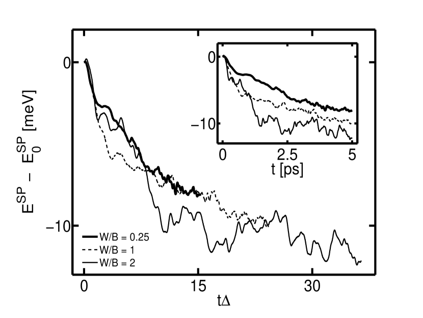
Figure 1: Total single particle energy as a function of time. The inset shows the raw data, in the main panel time is rescaled with the mean level spacing.

The total single particle energy decreases from its initial value with a rate depending on the mean level spacing of single-particle states $\Delta\equiv(W+B)/N/\hbar$ ($\hbar=0.658$ meVps) that results in a roughly universal behavior when time is rescaled accordingly.

The configuration average is possible only for quantities like the single particle energy, $E^{\mathrm{SP}}$ or the standard deviation, $\sigma$. On the other hand, $n_{\alpha\beta}$ corresponds to the eigenstates ${\alpha}$ and ${\beta}$ and the related eigenenergies, which are strongly dependent on the particular disorder realization. I.e., even the same $\alpha$ and $\beta$ refer to different eigenstates, which leads to non-comparable $n_{\alpha\beta}$ for different realizations.

Now let us turn towards the evaluation of the relaxation rate, $\Gamma$, which is defined via the assumption that $\sigma(t)$ decreases exponentially in the short-time regime of the dynamics, i.e.,

$$\sigma(t)=\sigma_{0}e^{-\Gamma t}\,.$$ (18)

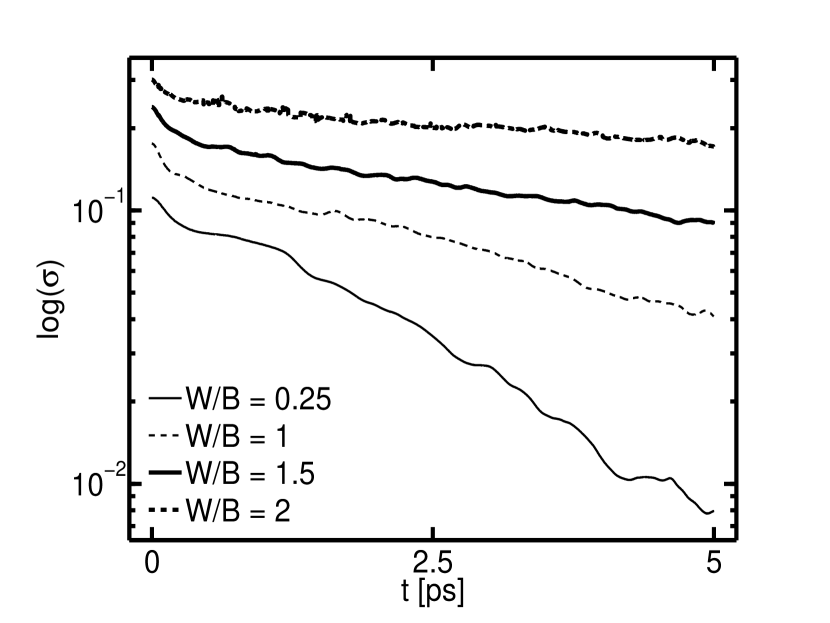
Figure 2: Error to a fit to a Fermi–Dirac distribution for a fixed interaction strength, $U_{0}=B=32$ meV for several values of disorder strength.

Indeed, our assumption is corroborated by the numerical simulations, shown in Fig. 2. The figure shows the fall–off of the deviation $\sigma$ as a function of time on a semi-log plot for several values of disorder in units of the bare bandwidth, $B=4J$. [As we have fixed the value of $J=8$ meV the bare bandwidth is $B=32$ meV. Hence the timestep for the integration in Eq. (14) was chosen to be $\delta t\approx 1$ fs.]

Thus it is reasonable to determine $\Gamma$ for various disorder and interaction strength values, both of which are measured in units of the bare bandwidth, $B=4J$. The results of these calculations are shown in Fig. 3, where $\Gamma$ is plotted as a function of disorder strength. The different lines belong to different interaction strengths. The rate $\Gamma$ is also given in units of $B$.

The inset in Fig. 3 contains the raw data which after a rescaling as $(U_{0}/B)^{c}$ is shown in the main panel, where $c\approx 1.6$. A similar scaling of the relaxation rate was found in [8], however with an exponent closer to the value of 2, but more work needs to be done to understand the nature of these scaling exponents. Clearly in Fig. 2 the case with low interaction strength deviates from the major trend substantially.

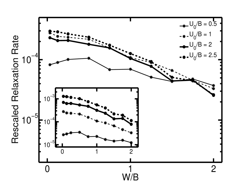
Figure 3: Relaxation Rate $\Gamma$ as a function of disorder strength for various interaction strengths. Data after rescaling as $(U_{0}/B)^{c}$, $c\approx 1.6$ is plotted in the main panel. The inset shows the raw data as a function of $W/B$.

5 Summary

In the present work we have shown that the interplay of both the disorder and the long-range interaction can be investigated on the same footing in order to study the relaxation process of an initially non-equilibrium one-particle occupation distribution towards an equilibrium one. The numerical solution of the equation of motion of the density matrix yields an exponential form for the deviation of the distribution from a Fermi-Dirac one. Additionally we found that the total single-particle energy gradually decreases as a function of time. This way the relaxation process in a completely closed system is possible via the rearrangement of the energy into other components of the otherwise constant total energy. A similar result has been found in [8], which, however, contained a phenomenological coupling to an environment. Morevoer, in the present calculation the off-diagonal matrix elements of the density matrix play an important role.

The results indicate that further advances can be achieved by improving the present method. In a subsequent work the effect of higher order correlations will be investigated, as well as the case of short ranged interaction.

P. B. and H. S. gratefully acknowledge the financial support by the European Commission, Marie Curie Excellence Grant MEXT-CT-2005-023778 (Nanoelectrophotonics). I.V. thanks for financial support from OTKA (Hungarian Research Fund) under Contracts No. T46303 and from European Commission Contract No. MRTN-CT-2003-504574.

References

- [1] F. Evers and A.D. Mirlin, arXiv:0707.4378; C. DiCastro and R. Raimondi, in: Proceedings of the International School of Physics ”Enrico Fermi”, Varenna, Italy, 2003, (IOS Press, Bologna, 2004), pp. 259-333.
- [2] D. M. Basko, I. L. Aleiner, and B. L. Altshuler, Ann. Phys. 321, 1126 (2006).
- [3] I. L. Aleiner, B. L. Altshuler, and M. E. Gershenson, Waves in Rand. Med. 9, 201 (1999).
- [4] M. Kira, F. Jahnke, W. Hoyer, and S. W. Koch, Progress in Quantum Electronic, 23, No. 6, (1999).
- [5] T. Meier, P. Thomas, and S. W. Koch, Coherent Semiconductor Optics: From Basic Concepts to Nanostructure Applications (Springer-Verlag, Berlin, 2007).
- [6] P. Bozsoki et al., Phys. Rev. Letters, 97, 227402 (2006), arXiv:cond-mat/0611411.
- [7] P. Bozsoki et al., Journal of Luminescence, 124, 99 (2007), arXiv:cond-mat/0505207.
- [8] I. Varga et al., Phys. Rev. B, 68, 113104 (2003), arXiv:cond-mat/0211206.