Generalised compact spheres in electric fields

Abstract

We present exact solutions to the Einstein-Maxwell system of equations in spherically symmetric gravitational fields with a specified form of the electric field intensity. The condition of pressure isotropy yields a difference equation with variable, rational coefficients. In an earlier treatment this condition was integrated by first transforming it to a hypergeometric equation. We demonstrate that it is possible to obtain a more general class of solutions to the Einstein-Maxwell system both in the form of special functions and elementary functions. Our results contain particular solutions found previously including models of charged relativistic spheres and uncharged neutron star models.

1 Introduction

Exact solutions of the Einstein-Maxwell system are important in the description of relativistic astrophysical processes. In the presence of charge the gravitational collapse of a spherically symmetric matter configuration to a point singularity may be avoided Kra . Einstein-Maxwell solutions are important in studies involving the cosmic censorship hypothesis and the formation of naked singularities Jos . The presence of the electromagnetic field affects the values of the surface redshifts, luminosities and the maximum mass for charged stars as demonstrated by Sharma et al ShMuMa , Ivanov Iva and others. The analysis of Patel and Koppar PaKo , Patel et al PaTiSa , Tikekar and Singh TiSi , Gupta and Kumar GuKu , and Mukherjee Muk have shown that it is feasible to model charged superdense neutron stars with densities in the range of 10¹⁴ g cm^-3; these models generate bounds for the surface readshift, luminosity and stellar mass which are consistent with observation. Sharma et al ShKaMu studied cold compact spheres, Tikekar and Jotania TiJo analysed strange matter, Sharma and Mukherjee ShMu considered the equation of state of a compact X-ray binary pulsar Her X-1, and Sharma and Mukherjee Sha investigated stars composed of quark-diquark particles which are consistent with the presence of an electromagnetic field. Einstein-Maxwell solutions may be applied to the core envelope models of Thomas et al ThRaVi , Tikekar and Thomas TiTh , and Paul and Tikekar PaTi with an inner core surrounded by an outer layer. These references provide a sample as to why the Einstein-Maxwell system, describing the interior of a charged star, has attracted the attention of many researchers.

Our intention in this paper is two-fold. Firstly, we seek to model a charged relativistic sphere which is physically acceptable. We require that the gravitational, electromagnetic and matter variables are finite, continuous and well behaved in the stellar interior, the interior metric should match smoothly with the exterior Reissner-Nordstrom metric, the speed of sound is less that the speed of light, and the solution is stable with respect to radial perturbations. Secondly, we seek to regain an uncharged solution of Einstein equations which satisfy the relevant physical criteria when the electric field vanishes. This ensures that a neutral relativistic star is regainable as a stable equilibrium state. We seek to construct a model, with limiting uncharged stars as known exact solutions, that exactly satisfies the Einstein-Maxwell systems. This ideal is not easy to achieve in practice and only a few examples with the required two features have been found thus far. Recently Hansraj and Maharaj HaMa , Thirukkanesh and Maharaj ThMa , and Komathiraj and Maharaj KoMa , KoMah found charged relativistic fluid spheres which regain neutral compact stars for particular parameter values.

Our objective is to find new solutions of the Einstein-Maxwell system that satisfy the physical criteria given above, and necessarily contains a neutral stellar solution. Our approach here complements the approach of Thirukkanesh and Maharaj ThMa who presented exact solutions to the Einstein-Maxwell equations; this family of solutions can be written in terms of elementary functions and reduces to the well known uncharged stellar model of Durgapal and Bannerji DuBa . The approach in ThMa introduces a transformation that reduces the condition of pressure isotropy to a hypergeometric equation. The transformation utilised in ThMa does produce new exact models but restricts the classes of solutions that are possible because of constraints placed on particular parameters. In this paper we do not transform the condition of pressure isotropy to the hypergeometric equation but are still in a position to integrate the field equations. A new class of Einstein-Maxwell solutions are found that contain familiar uncharged models which are regainable for different choices of the metric function and the electric field. In Section 2, we express the Einstein-Maxwell field equations for the static spherically symmetric line element as an equivalent set of differential equations utilising a transformation from DuBa . We choose particular forms for one of the gravitational potentials and the electric field intensity. This enables us to obtain the condition of pressure isotropy in the remaining gravitational potential which facilitates the integration process. In Section 3, we assume a solution in a series form which yields recurrence relations, which we manage to solve from first principles. It is then possible to exhibit exact solutions to the Einstein-Maxwell system. Solutions in terms of elementary functions are possible for particular parameter values. In Section 4, we present two linearly independent classes of solutions as combination of polynomials and algebraic functions. In addition we show that it is possible to express the general solution of the Einstein-Maxwell system in terms of elementary functions. We regain some solutions found previously from our general solutions in Section 5. In Section 6, we summarise the results found and present plots illustrating the behaviour of the matter variables.

2 The isotropic equations

We take the line element for static spherically symmetric spacetimes to be

$$ds^{2}=-e^{2\nu(r)}dt^{2}+e^{2\lambda(r)}dr^{2}+r^{2}(d\theta^{2}+\sin^{2}\theta d\phi^{2})$$ (1)

where $\nu(r)$ and $\lambda(r)$ are arbitrary functions. For charged perfect fluids, the Einstein-Maxwell field equations can be expressed as follows

$$\frac{1}{r^{2}}[r(1-e^{-2\lambda})]^{\prime} = \rho+\frac{1}{2}E^{2}$$ (2a)

$$\frac{-1}{r^{2}}(1-e^{-2\lambda})+\frac{2\nu^{\prime}}{r}e^{-2\lambda} = p-\frac{1}{2}E^{2}$$ (2b)

$$e^{-2\lambda}\left(\nu^{\prime\prime}+{\nu^{\prime}}^{2}+\frac{\nu^{\prime}}{r}-\nu^{\prime}\lambda^{\prime}-\frac{\lambda^{\prime}}{r}\right) = p+\frac{1}{2}E^{2}$$ (2c)

$$\sigma = \frac{1}{r^{2}}e^{-\lambda}(r^{2}E)^{\prime}$$ (2d)

for the geometry described by (1). The energy density $\rho$ and the pressure $p$ are measured relative to the comoving fluid 4-velocity $u^{a}=e^{-\nu}\delta^{a}_{0}$, $E$ is the electric field intensity, $\sigma$ is the proper charge density, and primes denote differentiation with respect to $r$. In the system (2a)-(2d) we are using units where the coupling constant $\frac{8\pi G}{c^{4}}=1$ and the speed of light $c=1$. The field equations (2a)-(2d) govern the behaviour of the gravitational field for a charged perfect fluid. When $E=0$ we regain Einstein equations for a neutral fluid.

An equivalent form of the field equations is generated if we introduce the transformation

$$A^{2}y^{2}(x)=e^{2\nu(r)},~{}~{}~{}Z(x)=e^{-2\lambda(r)},~{}~{}~{}x=Cr^{2}$$ (3)

where $A$ and $C$ are arbitrary constants. Under the transformation (3), the system (2) becomes

$$\frac{1-Z}{x}-2\dot{Z} = \frac{\rho}{C}+\frac{E^{2}}{2C}$$ (4a)

$$4Z\frac{\dot{y}}{y}+\frac{Z-1}{x} = \frac{p}{C}-\frac{E^{2}}{2C}$$ (4b)

$$4Zx^{2}\ddot{y}+2\dot{Z}x^{2}\dot{y}+\left(\dot{Z}x-Z+1-\frac{E^{2}x}{C}\right)y = 0$$ (4c)

$$\frac{\sigma^{2}}{C} = \frac{4Z}{x}(x\dot{E}+E)^{2}$$ (4d)

where dots denote differentiation with respect to the variable $x$. The particular representation of the Einstein-Maxwell system as given in (4a)-(4d) may be easier to integrate in certain situation as demonstrated by Hansraj and Maharaj HaMa and Komathiraj and Maharaj KoMah among others. To integrate the system (4) it is necessary to specify two of the variables $y,~{}Z,~{}\rho,~{}p$ or $E$. In our approach we choose $Z$ and $E$ on physical grounds. The remaining quantities are then obtained from the rest of the system (4).

In the integration procedure we make the choice

$$Z=\frac{1+kx}{1+x}$$ (5)

where $k$ is a real constant. For the choice (5) the line element (1) becomes

$$ds^{2}=-A^{2}y^{2}dt^{2}+\frac{1+x}{4Cx(1+kx)}dx^{2}+\frac{x}{C}(d\theta^{2}+\sin^{2}\theta d\phi^{2})$$

and we need to find the function $y(x)$. The form (5) ensures that the metric function behaves as

$$e^{2\lambda}=1+O(r^{2})$$

near $r=0$. In fact this is a sufficient condition for a static fluid sphere to be regular at the centre as pointed out by Maartens and Maharaj MaMa . The choice (5) ensures that the function is finite at the centre, remains regular and is well behaved in the stellar interior. This form contains particular solutions studied previously; for example when $k=-\frac{1}{2}$ we regain the neutron star model of Durgapal and Bannerji DuBa . The choice (5) ensures that charged spheres found as exact solutions of the Einstein-Maxwell system will contain physically reasonable uncharged models when $E=0$.

On substituting (5) in (4c) we obtain

$$4(1+kx)(1+x)\ddot{y}+2(k-1)\dot{y}+\left[(1-k)-\frac{E^{2}(1+x)^{2}}{Cx}\right]y=0$$ (6)

which is the condition of pressure isotropy. The solution of the Einstein-Maxwell system (4), for the form (5), depends on the integrability of (6). It is necessary to specify the electric field intensity $E$ to integrate (6). A variety of choices for $E$ is possible but only a few are physically reasonable which generate closed form solutions. We can reduce (6) to simpler form if we let

$$\frac{E^{2}}{C}=\frac{\alpha x}{(1+x)^{2}}$$ (7)

where $\alpha$ is a constant. The form for $E^{2}$ in (7) vanishes at the centre of the star, and remains continuous and bounded in the interior of the star for a wide range of values of the parameter $\alpha$. Thus the choice of $E^{2}$ is physically reasonable and useful in the gravitational analysis of charged spheres. When $\alpha=0$ there is no charge, and we regain uncharged stellar solutions such as the neutron star model of Durgapal and Bannerji DuBa for the parameter value $k=-\frac{1}{2}$. Note that the same form for the electric field intensity (7) was utilised by Hansraj and Maharaj HaMa and Thirukkanesh and Maharaj ThMa . For this form of $E^{2}$ a comprehensive physical analysis was performed by Hansraj and Maharaj HaMa for charged spheres when $k=0$. They demonstrated that all criteria for physical acceptability were satisfied including the fact that the speed of sound is less that the speed of light. We expect that this form for the electric field intensity, with the generalised potential (5), will provide a more general class of charged relativistic spheres with desirable physical features.

Upon substituting the choice (7) in equation (6) we obtain

$$4(1+kx)(1+x)\ddot{y}+2(k-1)\dot{y}+(1-k-\alpha)y=0$$ (8)

which is the master equation for the system (4). Thirukkanesh and Maharaj ThMa introduced the transformation

$$1+x=KX,~{}~{}~{}~{}~{}K=\frac{k-1}{k},~{}~{}~{}~{}~{}Y(X)=y(x)$$

so that (8) becomes

$$4X(1-X)\frac{d^{2}Y}{dX^{2}}-2\frac{dY}{dX}+(K+\tilde{\alpha})Y=0,~{}~{}~{}\tilde{\alpha}=\frac{\alpha}{k}$$

which is a special case of the hypergeometric equation. It is possible to integrate this hypergeometric equation. However it is important to note that the possible solutions are restricted as $k\neq 0$ and $k\neq 1$ because of the transformation used. We demonstrate in Section 3 that we can accommodate $k=0$ and $k=1$ in a wider class of solutions.

3 Master Equation

It is convenient to introduce the new variable $z=1+x$ in (8) to yield

$$4z(1-k+kz)\frac{d^{2}\tilde{y}}{dz^{2}}+2(k-1)\frac{d\tilde{y}}{dz}+(1-k-\alpha)\tilde{y}=0$$ (9)

where we have set $\tilde{y}=y(z)$. Two categories of solution are possible for $k=1$ and $k\neq 1$.

Case I : $k=1$
In this case (9) becomes the Euler-Cauchy equation with solution

$$y=c_{1}(1+x)^{(1+\sqrt{1+\alpha})/2}+c_{2}(1+x)^{(1-\sqrt{1+\alpha})/2}$$ (10)

where $c_{1},~{}c_{2}$ are constants. From (4a)-(4d), (5) and (10) we can show that the solution to the Einstein-Maxwell system, for our specific choices of $Z$ and $E$, becomes

$$e^{2\lambda} = 1$$ (11a)

$$e^{2\nu} = A^{2}[c_{1}(1+x)^{(1+\sqrt{1+\alpha})/2}+c_{2}(1+x)^{(1-\sqrt{1+\alpha})/2}]^{2}$$ (11b)

$$\rho = -\frac{\alpha Cx}{2(1+x)^{2}}$$ (11c)

$$p = \frac{2C[c_{1}(1+\sqrt{1+\alpha})(1+x)^{\sqrt{1+\alpha}}+c_{2}(1-\sqrt{1+\alpha})]}{(1+x)[c_{1}(1+x)^{\sqrt{1+\alpha}}+c_{2}]}+\frac{\alpha Cx}{2(1+x)^{2}}$$ (11d)

$$E^{2} = \frac{\alpha Cx}{(1+x)^{2}}$$ (11e)

in terms of the variable $x$. Observe that this case is not regainable from Thirukkanesh and Maharaj ThMa as $k\neq 1$ in their transformation. We do not pursue this case further as $\rho<0$.

Case II : $k\neq 1$
As the point $z=0$ is a regular singular point of (9), there exist two linearly independent solutions of the form of a power series with centre $z=0$. These solutions can be generated using the method of Frobenius. Therefore we can write

$$\tilde{y}=\sum_{i=0}^{\infty}a_{i}z^{i+b},~{}~{}~{}a_{0}\neq 0$$ (12)

where $a_{i}$ are the coefficients of the series and $b$ is a constant. For a legitimate solution we need to determine the coefficients $a_{i}$ as well as the parameter $b$. On substituting (12) in to (9) we obtain

$$2a_{0}b(1-k)(2b-3)z^{b-1}$$ (13)

$$+ \sum_{i=0}^{\infty}\{2(1-k)(i+b+1)(2i+2b-1)a_{i+1}$$

$$+ [4k(i+b)(i+b-1)+(1-k-\alpha)]a_{i}\}z^{b+i}=0$$

in increasing powers of $z$. For equation (13) to hold for all powers of $z$ in the interval of convergence we require

$$2a_{0}b(1-k)(2b-3) = 0$$ (14a)

$$a_{i+1} = \frac{4k(i+b)(i+b-1)+(1-k-\alpha)}{2(k-1)(i+b+1)(2i+2b-1)}a_{i},~{}~{}~{}i\geq 0$$ (14b)

Since $a_{0}\neq 0$ and $k\neq 1$, we have from (14a) that $b=0$ or $b=\frac{3}{2}$. Equation (14b) is the basic difference equation governing the structure of the solution. It is possible to express the coefficient $a_{i}$ in terms of the leading coefficient $a_{0}$ by establishing a general structure for the coefficients by considering the leading terms. These coefficients generate the pattern

$$a_{i+1}=\prod_{p=0}^{i}\frac{4k(p+b)(p+b-1)+(1-k-\alpha)}{2(k-1)(p+b+1)(2p+2b-1)}a_{0}$$ (15)

where we have utilised the conventional symbol $\prod$ to denote multiplication. It is easy to establish that the result (15) holds for all positive integers $p$ using the principle of mathematical induction.

Now it is possible to generate two linearly independent solutions to (9) with the help of (12) and (15). For the parameter value $b=0$ we obtain the first solution

$$\tilde{y}_{1}=a_{0}\left[1+\sum_{i=0}^{\infty}\prod_{p=0}^{i}\frac{4kp(p-1)+(1-k-\alpha)}{2(k-1)(p+1)(2p-1)}z^{i+1}\right]$$ (16)

For the parameter value $b=\frac{3}{2}$ we obtain the second solution

$$\tilde{y}_{2}=a_{0}z^{3/2}\left[1+\sum_{i=0}^{\infty}\prod_{p=0}^{i}\frac{k(2p+3)(2p+1)+(1-k-\alpha)}{(k-1)(2p+5)(2p+2)}z^{i+1}\right]$$ (17)

Thus we can write the general solution to the differential equation (9), for the choice of the electric field given in (7), as

$$\tilde{y}=\tilde{c}_{1}\tilde{y}_{1}+\tilde{c}_{2}\tilde{y}_{2}$$ (18)

where $\tilde{c}_{1},~{}\tilde{c}_{2}$ are arbitrary constants, and $\tilde{y}_{1}$ and $\tilde{y}_{2}$ are given in (16) and (17) respectively. In terms of the variable $x$ we can write (18) as

$$y = c_{1}\left[1+\sum_{i=0}^{\infty}\prod_{p=0}^{i}\frac{4kp(p-1)+(1-k-\alpha)}{2(k-1)(p+1)(2p-1)}(1+x)^{i+1}\right]$$ (19)

$$+ c_{2}(1+x)^{3/2}\left[1+\sum_{i=0}^{\infty}\prod_{p=0}^{i}\frac{k(2p+3)(2p+1)+(1-k-\alpha)}{(k-1)(2p+5)(2p+2)}(1+x)^{i+1}\right]$$

$$= c_{1}y_{1}(x)+c_{2}y_{2}(x)$$

where we have set $c_{1}=\tilde{c}_{1}a_{0}$ and $c_{2}=\tilde{c}_{2}a_{0}$ for simplicity. The solution to the Einstein-Maxwell system (4a)-(4d), for our specific choices of $Z$ and $E$, can now be written as

$$e^{2\lambda} = \frac{1+x}{1+kx}$$ (20a)

$$e^{2\nu} = A^{2}y^{2}$$ (20b)

$$\frac{\rho}{C} = \frac{(1-k)(3+x)}{(1+x)^{2}}-\frac{\alpha x}{2(1+x)^{2}}$$ (20c)

$$\frac{p}{C} = 4\frac{(1+kx)}{(1+x)}\frac{\dot{y}}{y}+\frac{(k-1)}{(1+x)}+\frac{\alpha x}{2(1+x)^{2}}$$ (20d)

$$\frac{E^{2}}{C} = \frac{\alpha x}{(1+x)^{2}}$$ (20e)

in terms of the variable $x$. The form of the exact solution (20a)-(20e) has a similar structure to the general solution of Thirukkanesh and Maharaj ThMa ; however it is important to realise that our solution is a new result because the series in (19) is different. In addition note that $k=0$ is allowed in (20a)-(20e) unlike the result of Thirukkanesh and Maharaj ThMa ; our result can be interpreted as a generalisation.

4 Elementary solutions

The general solution (19) is given in the form of a series which define special functions. For particular values of the parameters involved it is possible for the general solution to be written in terms of elementary functions which is a more desirable form for the physical description of a charged relativistic star. We find two linearly independent solutions, in terms of elementary functions, in this section for the differential equation (9).

4.1 First solution

On substituting $b=0$ and setting $1-k-\alpha=-4kn(n-1)$ in (14b) we obtain

$$a_{i+1}=\frac{4k}{1-k}\frac{(n-i)(n+i-1)}{(2i+2)(2i-1)}a_{i},~{}~{}~{}i\geq 0$$ (21)

It is easy to see from (21) that $a_{n+1}=0$. Clearly the subsequent coefficients $a_{n+2},~{}a_{n+3},\\ ~{}a_{n+4},.~{}.~{}.$ vanish. Equation (21) has the solution

$$a_{i}=-\left(\frac{4k}{1-k}\right)^{i}\frac{n(n-1)(2i-1)(n+i-2)!}{(2i)!(n-i)!}a_{0},~{}~{}~{}0\leq i\leq n$$ (22)

Then from (12) (when $b=0$) and (22), we obtain

$$\tilde{y}_{1}=a_{0}\left[1-\sum_{i=1}^{n}\left(\frac{4k}{1-k}\right)^{i}\frac{n(n-1)(2i-1)(n+i-2)!}{(2i)!(n-i)!}z^{i}\right]$$ (23)

for $1-k-\alpha=-4kn(n-1)$.

On substituting $b=\frac{3}{2}$ and setting $1-k-\alpha=-k(2n+3)(2n+1)$ in (14b) we obtain

$$a_{i+1}=\frac{4k}{1-k}\frac{(n-i)(n+i+2)}{(2i+5)(2i+2)}a_{i},~{}~{}~{}i\geq 0$$ (24)

We observe from (24) that $a_{n+1}=0$. Consequently the remaining coefficients $a_{n+2},~{}a_{n+3},\\ ~{}a_{n+4},~{}.~{}.~{}.$ vanish. Equation (24) may be solved to yield

$$a_{i}=3\left(\frac{4k}{1-k}\right)^{i}\frac{(2i+2)(n+i+1)!}{(n+1)(2i+3)!(n-i)!}a_{0},~{}~{}~{}0\leq i\leq n$$ (25)

Now from (12) (when $b=\frac{3}{2}$) and (25), we obtain

$$\tilde{y}_{1}=a_{0}z^{3/2}\left[1+3\sum_{i=1}^{n}\left(\frac{4k}{1-k}\right)^{i}\frac{(2i+2)(n+i+1)!}{(n+1)(2i+3)!(n-i)!}z^{i}\right]$$ (26)

for $1-k-\alpha=-k(2n+3)(2n+1)$.

The polynomial and algebraic functions (23) and (26) comprise the first solution to the differential equation (9) for appropriate values of $k$ and $\alpha$.

4.2 Second solution

We can find the second solution of (9) using the method of reduction of order in principle. However this proves to be difficult in practice because of the complicated form of the first solution given in (23) and (26). We utilise a transformation to first simplify (9) before seeking the second solution. We take the second solution of (9) to be of the form

$$\tilde{y}=(1-k+kz)^{1/2}u(z)$$ (27)

when $u(z)$ is an arbitrary polynomial. Special cases of (27) are known to solve (9) which motivates the algebraic form for $\tilde{y}$ as a generic second solution to the differential equation (9). On substituting $\tilde{y}$ in (9) we obtain

$$4z(1-k+kz)\frac{d^{2}u}{dz^{2}}+[4kz+2(k-1)]\frac{du}{dz}+(1-2k-\alpha)u=0$$ (28)

which is linear differential equation for $u(z)$.

As in Section 4.1 it is possible to find solutions in terms of polynomials, and product of polynomials with algebraic functions for $u(z)$ for certain values of the parameters $k$ and $\alpha$. As the point $z=0$ is a regular singular point of (28), there exist two linearly independent solutions of the form of the power series with centre $z=0$. Thus we assume

$$u=\sum_{i=0}^{\infty}c_{i}z^{i+d}$$ (29)

where the constants $c_{i}$ are the coefficients of the series and $d$ is the constant. Substituting (29) in (28) we obtain

$$2c_{0}d(1-k)(2d-3)z^{d-1}$$ (30)

$$+ \sum_{i=0}^{\infty}\{2(1-k)(i+d+1)(2i+2d-1)c_{i+1}$$

$$+ [4k(i+d)^{2}+(1-2k-\alpha)]c_{i}\}z^{i+d}=0$$

For equation (30) to hold true for all $z$ we require that

$$2c_{0}d(1-k)(2d-3) = 0$$ (31a)

$$c_{i+1} = \frac{4k(i+d)^{2}+(1-2k-\alpha)}{2(k-1)(i+d+1)(2i+2d-1)}c_{i},~{}~{}~{}i\geq 0$$ (31b)

Since $c_{0}\neq 0$ and $k\neq 1$ we have from (31a) that $d=0$ or $d=\frac{3}{2}$. Equation (31b) is the linear recurrence relation governing the structure of the solution.

On substituting $d=0$ and setting $1-k-\alpha=-k(2n+1)(2n+3)$ in (31b) we obtain

$$c_{i+1}=\left(\frac{4k}{1-k}\right)\frac{(n-i+1)(n+i+1)}{(2i+2)(2i-1)}c_{i},~{}~{}~{}i\geq 0$$ (32)

From (32) we have that $c_{n+2}=0$ and subsequent coefficients $c_{n+3},~{}c_{n+4},~{}c_{n+5},~{}.~{}.~{}.$ vanish. Then (32) has the solution

$$c_{i}=-\left(\frac{4k}{1-k}\right)^{i}\frac{(n+1)(2i-1)(n+i)!}{(2i)!(n-i+1)!}c_{0},~{}~{}~{}0\leq i\leq n+1$$ (33)

Then from (29) (when $d=0$) and (33) we obtain

$$\tilde{y}_{2}=c_{0}(1-k+kz)^{1/2}\left[1-\sum_{i=1}^{n+1}\left(\frac{4k}{1-k}\right)^{i}\frac{(n+1)(2i-1)(n+i)!}{(2i)!(n-i+1)!}z^{i}\right]$$ (34)

for $1-k-\alpha=-k(2n+1)(2n+3)$.

On substituting $d=\frac{3}{2}$ and setting $1-k-\alpha=-4kn(n-1)$ in (31b) we obtain

$$c_{i+1}=\left(\frac{4k}{1-k}\right)\frac{(n+i+1)(n-i-2)}{(2i+2)(2i+5)}c_{i},~{}~{}~{}i\geq 0$$ (35)

From (35) we have that $c_{n-1}=0$ and subsequent coefficients $c_{n},~{}c_{n+1},~{}c_{n+2},~{}.~{}.~{}.$ vanish. The equation (35) has the solution

$$c_{i}=3\left(\frac{4k}{1-k}\right)^{i}\frac{(2i+2)(n+i)!}{n(n-1)(2i+3)!(n-i-2)!}c_{0},~{}~{}~{}0\leq i\leq n-2$$ (36)

From (29) (when $d=\frac{3}{2}$) and (36) we obtain

$$\tilde{y}_{2}=c_{0}(1-k+kz)^{1/2}z^{3/2}\left[1+3\sum_{i=1}^{n-2}\left(\frac{4k}{1-k}\right)^{i}\frac{(2i+2)(n+i)!}{n(n-1)(2i+3)!(n-i-2)!}z^{i}\right]$$ (37)

for $1-k-\alpha=-4kn(n-1)$.

The algebraic solutions (34) and (37) comprise the second solution of the differential equation (9) which are clearly independent from (26) and (23).

4.3 Elementary functions

We have obtained one class of polynomial solution (23) and three classes of solutions (26), (34), and (37) in terms of product of polynomials and algebraic functions. The polynomial solution (23) and the product of polynomials with an algebraic function (26) generate the first solution. The second linearly independent solution is given by (34) and (37) which are products of polynomials and algebraic functions. By collecting these results we can express the general solution to (9) in two categories. We express the general solution in terms of the independent variable $x$. From (23) and (37) we write the first category as

$$y = A\left[1-\sum_{i=1}^{n}\left(\frac{4k}{1-k}\right)^{i}\frac{n(n-1)(2i-1)(n+i-2)!}{(2i)!(n-i)!}(1+x)^{i}\right]$$

$$+ B(1+kx)^{1/2}(1+x)^{3/2}\left[1+3\sum_{i=1}^{n-2}\left(\frac{4k}{1-k}\right)^{i}\frac{(2i+2)(n+i)!}{n(n-1)(2i+3)!(n-i-2)!}(1+x)^{i}\right]$$

for $1-k-\alpha=-4kn(n-1)$. From (26) and (34), the second category of solution has the form

$$y = A(1+x)^{3/2}\left[1+3\sum_{i=1}^{n}\left(\frac{4k}{1-k}\right)^{i}\frac{(2i+2)(n+i+1)!}{(n+1)(2i+3)!(n-i)!}(1+x)^{i}\right]$$

$$+ B(1+kx)^{1/2}\left[1-\sum_{i=1}^{n+1}\left(\frac{4k}{1-k}\right)^{i}\frac{(n+1)(2i-1)(n+i)!}{(2i)!(n-i+1)!}(1+x)^{i}\right]$$

for $1-k-\alpha=-k(2n+1)(2n+3)$. In the above $A$ and $B$ are arbitrary constants. Consequently we have demonstrated that elementary functions can be extracted from the general series (19) by restricting the parameter values $\alpha$ and $k$. The general solutions (4.3) and (4.3) have a very simple form. It is important to observe that the Einstein-Maxwell solutions (4.3) and (4.3) apply to both charged and uncharged relativistic stars. We regain neutral exact solutions, which may be possibly new, by setting $\alpha=0$.

5 Known cases

We may generate individual models for charged and uncharged stars found previously from our general class of solutions. These can be explicitly regained from the general series solution (19) or the elementary functions (4.3) and (4.3). We demonstrate that this is possible in the following cases:

Case I : Thirukkanesh and Maharaj charged stars
If we set $K=\frac{k-1}{k},~{}~{}\hat{\alpha}=\frac{\alpha}{k},~{}~{}c_{1}=d_{1}$ and $c_{2}=K^{-3/2}d_{2}$ then (19) can be written as

$$y = d_{1}\left[1+\sum_{i=0}^{\infty}\prod_{p=0}^{i}\frac{4p(p-1)-(K+\tilde{\alpha})}{2(p+1)(2p-1)}\left(\frac{1+x}{K}\right)^{i+1}\right]$$ (40)

$$+ d_{2}\left(\frac{1+x}{K}\right)^{3/2}\left[1+\sum_{i=0}^{\infty}\prod_{p=0}^{i}\frac{(2p+3)(2p+1)-(K+\tilde{\alpha})}{(2p+5)(2p+2)}\left(\frac{1+x}{K}\right)^{i+1}\right]$$

The Einstein-Maxwell solution (40) corresponds to the charged model of Thirukkanesh and Maharaj ThMa . However note that $k\neq 0$ and $k\neq 1$ in (40). In our wider class of solutions (19) it is permitted that $k=0$; the exact solution (10) corresponds to the case $k=1$. The Thirukkanesh-Maharaj charged stars contain neutron star models found previously including the Durgapal and Bannerji model, and they are consequently physically reasonable.

Case II : Hansraj and Maharaj charged stars
If we set $k=0$ then it is possible after some manipulation, to write (19) in the form

$$y = c_{1}\left[1+\sum_{i=0}^{\infty}\frac{(-1)^{i}(2i+1)}{(2i+2)!}[(1-\alpha)(1+x)]^{i+1}\right]$$ (41)

$$+ c_{2}(1+x)^{3/2}\left[1+\sum_{i=0}^{\infty}\frac{3(-1)^{i+1}(2i+4)}{(2i+5)!}[(1-\alpha)(1+x)]^{i+1}\right]$$

$$= c_{1}\left[1-\sum_{i=0}^{\infty}(-1)^{i}\left(\frac{1}{(2i+2)!}-\frac{1}{(2i+1)!}\right)[\sqrt{(1-\alpha)(1+x)}]^{2(i+1)}\right]$$

$$+ \frac{3c_{2}}{(1-\alpha)^{3/2}}[\sqrt{(1-\alpha)(1+x)}]^{3}$$

$$\times \left[\frac{1}{3}-\sum_{i=0}^{\infty}(-1)^{i+1}\left(\frac{1}{(2i+5)!}-\frac{1}{(2i+4)!}\right)[\sqrt{(1-\alpha)(1+x)}]^{2(i+1)}\right]$$

It is interesting to observe that the last equation above can be expressed in terms of trigonometric functions. Then it is easy to show that (41) can be written in the form

$$y = c_{1}[\cos\sqrt{(1-\alpha)(1+x)}+\sqrt{(1-\alpha)(1+x)}\sin\sqrt{(1-\alpha)(1+x)}]$$ (42)

$$+ \frac{3c_{2}}{(1-\alpha)^{3/2}}[\sin\sqrt{(1-\alpha)(1+x)}-\sqrt{(1-\alpha)(1+x)}\cos\sqrt{(1-\alpha)(1+x)}]$$

$$= [d_{1}+d_{2}\sqrt{(1-\alpha)(1+x)}]\sin\sqrt{(1-\alpha)(1+x)}$$

$$+ [d_{2}-d_{1}\sqrt{(1-\alpha)(1+x)}]\cos\sqrt{(1-\alpha)(1+x)}$$

where we have set $d_{1}=\frac{3c_{2}}{(1-\alpha)^{3/2}}$ and $d_{2}=c_{1}$. The Einstein-Maxwell solution (42) is the same as the charged model of Hansraj and Maharaj HaMa . Note that our solution (42) corrects a minor misprint in the result of HaMa . The Hansraj-Maharaj charged stars were comprehensively studied in HaMa ; it was demonstrated that their model produced a charged relativistic sphere that satisfied all physical criteria. In particular the speed of sound was less that the speed of light and causality is maintained.

Case III : Finch and Skea neutron stars
If we set $k=0$ and $\alpha=0$, and follows the procedure outlined for Case II, then (19) becomes

$$y = [d_{1}+d_{2}\sqrt{(1+x)}]\sin\sqrt{(1+x)}+[d_{2}-d_{1}\sqrt{(1+x)}]\cos\sqrt{(1+x)}$$ (43)

where we have set $d_{1}=3c_{2}$ and $d_{2}=c_{1}$. Alternatively we can obtain the result (43) directly from (42) with $\alpha=0$. The exact solution (43) is the neutron star model of Finch and Skea FiSk . The Finch-Skea model satisfies all the physical conditions for an isolated spherically symmetric stellar source, and consequently has been utilised by many researchers to model neutron stars.

Case IV : Durgapal and Bannerji neutron stars
If we set $\alpha=0$ and $k=-\frac{1}{2}(n=0)$, then (4.3) becomes

$$y=c(1+x)^{3/2}+d(2-x)^{1/2}(5+2x)$$ (44)

where we have set $c=A$ and $d=\frac{B}{3\sqrt{2}}$. The exact solution (44) was first found by Durgapal and Bannerji DuBa . The Durgapal-Bannerji solution has been widely applied as a relativistic model for neutral stars with superdense matter.

6 Discussion

We have found new solutions (20) to the Einstein-Maxwell system (4) by utilising the method of Frobenius for an infinite series; a form for one of the gravitational potentials was assumed and the electric field intensity was specified. These solutions are given in terms of special functions. For particular values of the parameters involved it is possible to write the solution in terms of elementary functions: polynomials and products of polynomials and algebraic functions. The electromagnetic field may vanish in the general series solutions and we can regain uncharged solutions. Thus our approach has the advantage of necessarily containing a neutral stellar solution. The charged model of Thirukkanesh and Maharaj ThMa , the charged spheres of Hansraj and Maharaj HaMa , the uncharged neutron star model of Finch and Skea FiSk , and the uncharged superdense star of Durgapal and Bannerji DuBa are contained as special cases in our class of solutions to the Einstein-Maxwell system. The simple form of the solutions found facilitates the analysis of the physical features of a charged sphere.

We are now in a position to investigate graphically the behaviour of the matter variables in the stellar interior for particular choices of the parameter values in (20). We have generated figure 1 with the assistance of the software package Mathematica. For simplicity we make the choices $A=B=C=1$, $k=\frac{1}{4}$ and $\alpha=\frac{3}{2}$, over the interval $0\leq r\leq 1$, to generate the relevant plots. In figure 1, plot A represents the energy density $\rho$, plot B represents the pressure $p$, and plot $C$ represents the electric field intensity $E^{2}$. It can easily be seen that these matter variables remain regular in the interior of the star for $0\leq r\leq 1$. We observe that the energy density and the pressure are positive and monotonically decreasing functions in the interior of the star. The electric field intensity is positive and monotonically increasing for the interval of the plot. Thus the quantities $\rho$, $p$ and $E^{2}$ are continuous, regular and well behaved in the interior of the star. Consequently the solutions found in this paper are likely to be useful in the description of charged relativistic fluid spheres.

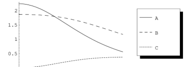
Figure 1: Plots of the energy density $\rho$, pressure $p$ and electric field $E^{2}$.

Acknowledgements

KK thanks the South Eastern University of Sri Lanka for granting study leave and the National Research Foundation and the University of KwaZulu-Natal for financial support. SDM acknowledges that this work is based upon research supported by the South African Research Chair Initiative of the Department of Science and Technology and the National Research Foundation.

References

- [1] Krasinski A 1997 Inhomogeneous Cosmological Models (Cambridge: Cambridge University Press)
- [2] Joshi P S 1993 Global Aspects in Gravitation and Cosmology (Oxford: Clarendan Press)
- [3] Sharma R, Mukherjee S and Maharaj S D 2001 Gen. Relat. Gravit. 33 999
- [4] Ivanov B V 2002 Phys. Rev. D 65 104001
- [5] Patel L K and Koppar S K 1987 Aust. J. Phys. 40 441
- [6] Patel L K, Tikekar R and Sabu M C 1997 Gen. Relat. Gravit. 29 489
- [7] Tikekar R and Singh G P 1998 Gravitation and Cosmology 4 294
- [8] Gupta Y K and Kumar M 2005 Gen. Relat. Gravit. 37 233
- [9] Mukherjee B 2001 Acta Phys. Hung. 13 243
- [10] Sharma R, Karmakar S and Mukherjee S 2006 Int. J. Mod. Phys. D 15 405
- [11] Tikekar R and Jotania K 2005 Int. J. Mod. Phys. D 14 1037
- [12] Sharma R and Mukherjee S 2001 Mod. Phys. Lett. A 16 1049
- [13] Sharma R and Mukherjee S 2002 Mod. Phys. Lett. A 17 2535
- [14] Thomas V O, Ratanpal B S and Vinodkumar P C 2005 Int. J. Mod. Phys. D 14 85
- [15] Tikekar R and Thomas V O 1998 Pramana - J. Phys. 50 95
- [16] Paul B C and Tikekar R 2005 Gravitation and Cosmology 11 244
- [17] Hansraj S and Maharaj S D 2006 Int. J. Mod. Phys. D 15 1311
- [18] Thirukkanesh S and Maharaj S D 2006 Class. Quantum Grav. 23 2697
- [19] Komathiraj K and Maharaj S D 2007 J. Math. Phys. 48 042501
- [20] Komathiraj K and Maharaj S D 2007 Gen. Relat. Gravit. Submitted
- [21] Durgapal M C and Bannerji R 1983 Phys. Rev. D 27 328
- [22] Finch M R and Skea J E F 1989 Class. Quantum Grav. 6 467
- [23] Maartens R and Maharaj M S 1990 J. Math. Phys. 31 151