Phase Transitions in Pressurised Semiflexible Polymer Rings

Abstract

We propose and study a model for the equilibrium statistical mechanics of a pressurised semiflexible polymer ring. The Hamiltonian has a term which couples to the algebraic area of the ring and a term which accounts for bending (semiflexibility). The model allows for self-intersections. Using a combination of Monte Carlo simulations, Flory-type scaling theory, mean-field approximations and lattice enumeration techniques, we obtain a phase diagram in which collapsed and inflated phases are separated by a continuous transition. The scaling properties of the averaged area as a function of the number of units of the ring are derived. For large pressures, the asymptotic behaviour of the area is calculated for both discrete and lattice versions of the model. For small pressures, the area is obtained through a mapping onto the quantum mechanical problem of an electron moving in a magnetic field. The simulation data agree well with the analytic and mean-field results.

I Introduction

Fluid vesicles obtained via the self-assembly of amphiphilic molecules exhibit a variety of shapes in thermal equilibrium. Such shapes can be understood in terms of the energy minimising configurations of a curvature Hamiltonian, under the constraints of fixed enclosed volume and surface areaCanham (1970); Helfrich (1973); Evans (1974). Shape changes arise when solutions of the Euler-Lagrange equations representing distinct shapes exchange stability. However, the non-linearity of these equations, if no special symmetries are assumed, necessitates purely numerical approaches. Further, while the curvature modulus in bilayer lipid membrane systems is often large, so that thermal fluctuations about the minimum free energy structure may be ignored, the more general problem of understanding the thermodynamics of such shape transitions is a formidable oneSeifert (1997).

The two-dimensional version of the vesicle problem is a polymer ring of fixed contour length, whose enclosed area $A$ is constrained through a coupling to a pressure difference term $p$. Leibler, Singh and Fisher (LSF) Leibler et al. (1987) performed a Monte Carlo and scaling study of two-dimensional vesicles, modelled as closed, planar, self-avoiding tethered chains, accounting for both pressure and bending rigidity. In this model, the ring polymer is obtained by connecting the centres of impenetrable particles of fixed radius with tethers of a fixed maximum length, while enforcing self-avoidance. LSF showed the existence of a phase transition at $p=0$, separating a branched polymer phase for $p<0$ from an inflated phase for $p>0$. At the transition point, the ring is described by a self avoiding polygon. Various fractal and non-fractal shapes that arise in these models have also been investigated Fisher (1989); Camacho and Fisher (1990).

Analytic studies of this class of models present many difficulties, arising principally from the self-avoidance constraint. Nevertheless, the relatively simple structure of the LSF model has stimulated a considerable body of work, largely in exact enumeration studies of lattice versions of the original continuum model and its variants van Rensburg (2000); Fisher et al. (1991); Bousquet-Mélou (1996); Guttmann and Lin (1992); Richard et al. (2001); Cardy (2001); Richard (2002); Richard et al. (2003); Rajesh and Dhar (2005). Most of these studies have concentrated on the behaviour of the system in the thermodynamic limit in the region $p\leq 0$. However, the $p>0$ case can exhibit interesting crossover behaviour for large but finite systems.

The consequences of relaxing the self-avoidance constraint were studied in Refs. Rudnick and Gaspari (1991); Gaspari et al. (1993); Marconi and Maritan (1993). In the models studied in these papers, the ring was allowed to intersect itself, with the pressure term coupled to the algebraic area Gaspari et al. (1993); Rudnick and Gaspari (1991) or to its square Marconi and Maritan (1993). The particles linked to form the polymer were coupled through harmonic springs Gaspari et al. (1993); Rudnick and Gaspari (1991), thus allowing for the extensibility of the chain. We shall refer to this model as the Extensible Self-Intersecting Ring (ESIR). The ESIR model can be solved exactly. The solution yields collapsed and inflated phases of the ring separated by a continuous phase transition that occurs at a critical value of an appropriately scaled pressureGaspari et al. (1993). However, the model has a major shortcoming in that the inflated phase is an unphysical one in which the ring expands to an infinite size. In a more realistic model, such an expansion would be limited by the finite size of individual link lengths.

The unphysical nature of the inflated phase in the ESIR model has been addressed in recent workHaleva and Diamant (2006), in which particles are joined by bonds of fixed length, as opposed to springs. The Hamiltonian has a term where the pressure couples to the algebraic area, as in the ESIR model. The transition survives as a continuous phase transition with mean-field exponents, separating collapsed and inflated regimes of the ring. We shall refer to this model as the Inextensible Self-Intersecting Ring (ISIR).

The model proposed in this paper incorporates a bending energy into the ISIR model along standard lines for semiflexible polymers. We retain the coupling of the signed pressure to the algebraic area noting, as argued in Haleva and Diamant (2006), that this difference, while vastly increasing the tractability of the problem, makes little difference to computations within the inflated phase.

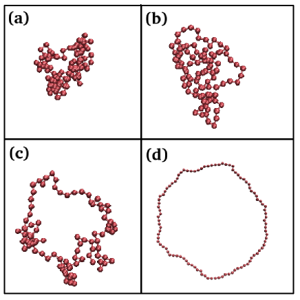
Figure 1: The collapsed to inflated phase transition as the pressure is increased. The different panels correspond to (a) $J=0$, $p<p_{c}$; (b) $J=2$, $p<p_{c}$; (c) $J=0$, $p=p_{c}$; and (d) $J=0$, $p>p_{c}$.

The continuum problem we address is the following. If the polymer chain is specified by the curve $\vec{r}(s)$, where $s$ is the arc-length along the curve, we consider the Hamiltonian

$$\mathcal{H}=-\frac{p}{2}\int_{0}^{L}ds\left(\vec{r}\times\frac{d\vec{r}}{ds}\right)\cdot\hat{z}+\frac{\kappa}{2}\int_{0}^{L}ds\left|\frac{d^{2}\vec{r}}{ds^{2}}\right|^{2}.$$ (1)

Here, $ds(\vec{r}\times d\vec{r}/ds)\cdot\hat{z}$ is the infinitesimal (signed) area which must be integrated over the internal variable $s$ to obtain the total algebraic area. The quantity $L=Na$ is the length of the polymer ring of $N$ units where $a$ is the size of the basic monomer. The continuum limit is taken such that $N\rightarrow\infty$ and $a\rightarrow 0$, keeping $L=Na$ fixed. The parameter $p=p_{in}-p_{out}$ represents the pressure differential between the inside and the outside of the ring and $\kappa$ is the bending rigidity of the chain. We measure energies in units of $k_{B}T$. The inextensibility constraint is imposed through

$$\hat{t}(s)=\left|\frac{d\vec{r}}{ds}\right|=1,$$ (2)

where $\hat{t}(s)$ is the unit tangent vector. When $p=0$, this model reduces to the worm-like chain model, with configurations constrained by the closure requirement.

We will work with two discretized versions of the above Hamiltonian. The first has $N$ particles in the continuum connected through fixed length links, forming a ring polymer whose equilibrium configurations are constrained by the pressurisation and bending energy terms above, but where the ring can intersect itself at no energy cost. We will refer to this version of our model as the “discrete model”. The second is a square lattice version of the same problem with the particles constrained to lie on the vertices of the lattice. We will refer to this version as the “lattice model”. We discuss the differences and similarities between the two versions.

We use a combination of analytic and numerical methods to study these models: Flory type scaling theory for the scaling of the area as a function of pressure, Monte Carlo simulations for different pressures and bending rigidity, mean field approaches and exact enumeration.

In Fig. 1 we show typical configurations obtained from Monte Carlo simulations of the discrete model in four limits. These are configuration snapshots across the collapsed to inflated phase transition, for different values of the bending rigidity $J$ of the discrete model ($J\propto\kappa$), as the pressure $p$ is varied. Fig. 1(a) shows the collapsed phase for the case where the bending energy is zero, while Fig. 1(b) illustrates a typical ring configuration at an intermediate value of the bending rigidity, but still within the collapsed regime. In Fig. 1(c), we show a typical configuration close to the transition between collapsed and inflated phases. Last, Fig. 1(d) illustrates the fully inflated ring.

We summarise our main results below. We show that there is a continuous phase transition in the scaled pressure $\hat{p}~{}(Np/4\pi)$ – bending rigidity ($J$) phase diagram, which separates a collapsed phase in which $\mbox{area}\propto N$, from an inflated phase in which $\mbox{area}\propto N^{2}$ (see Fig. 2). The phase boundary for the discrete model is obtained as $\hat{p}_{c}=[I_{0}(J)-I_{1}(J)]/[I_{0}(J)+I_{1}(J)]$, where the $I(J)$’s are modified Bessel functions. For the lattice model, the phase boundary is obtained as $\hat{p}_{c}=e^{-J}$.

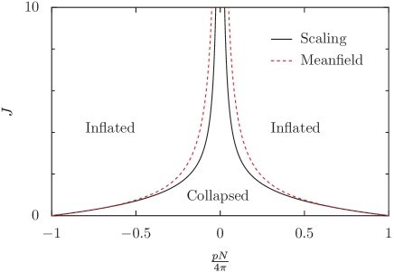
Figure 2: The phase boundary between collapsed and inflated phases for a semi-flexible polymer ring as obtained by two different methods, a scaling analysis based on Flory-type arguments and mean-field theory.

These results are obtained by first solving the $J=0$ case exactly and then incorporating the effects of a nonzero $J$ through a scaling argument. For the collapsed phase, the free energy for nonzero $J$ is calculated by the same method. In the inflated regime, we resort to mean field theories. We employ two types of mean-field theories: In the first, the inextensibility constraint is satisfied exactly but the closure condition is satisfied only on average. In the second, we impose the closure condition exactly but satisfy the inextensibility constraint only on average. The dependence of the area on $\hat{p}$ for $\hat{p}\rightarrow\infty$ is calculated. The behaviour near the transition line is obtained through a Flory type scaling theory.

The rest of the paper is organised as follows. In Sec. II we define our models more precisely. Section III contains the details of the numerical methods used, including the Monte Carlo and exact enumeration algorithms. In Sec. IV, we discuss a Flory-type scaling theory valid for the semi-flexible case. Section V describes mean-field approaches to this problem: (a) a simple density-matrix based single-site mean-field approach which captures the properties of the inflated phase to very high accuracy but is inadequate for the collapsed phase and (b), a less accurate harmonic spring mean-field theory, which is capable of describing both collapsed and inflated phases. In Sec. VI, we discuss the behaviour around the critical point in greater detail. Our Sec. VII contains results for the asymptotic behaviour of the area as well as a description of the appropriate scaling function for the area in the lattice case, as a function of $N$. Section VIII contains a summary and conclusions. In Appendix A we present a solution of the problem when $J=0$ by drawing an analogy with the quantum mechanical problem of the motion of an electron in a magnetic field.

II Model

Consider a closed chain of N monomers in two dimensions. Let the positions of the $j^{th}$ particle be denoted by the vector $\vec{r}_{j}$ and the corresponding tangent vectors by $\vec{t}_{j}=\vec{r}_{j+1}-\vec{r}_{j},\;j=1,2,\ldots,N.$ For a closed ring, $\vec{r}_{N+1}=\vec{r}_{1}$, or equivalently, $\sum_{i}\vec{t}_{i}=0$. The algebraic or signed area area $A_{s}$ enclosed by the ring is given by

$$A_{s}=\frac{1}{2}\sum_{i=1}^{N}(\vec{r}_{i}\times\vec{r}_{i+1})\cdot\hat{z}=\sum_{j=1}^{N}\sum_{k=1}^{j-1}(\vec{t}_{k}\times\vec{t}_{j})\cdot\hat{z}.$$ (3)

$A_{s}$ can be either positive or negative.

Coupling this algebraic area to pressure, we obtain the energy term,

$$H_{p}=-pA_{s}.$$ (4)

The bending energy cost can then be written down following standard procedures as

$$H_{b}=-J\sum_{i=1}^{N}\hat{t}_{i}\cdot\hat{t}_{i+1},$$ (5)

where the bending rigidity $J$ of the discrete model is proportional to the continuum bending rigidity and $\hat{t}$ is the unit vector in the direction of $\vec{t}$. The inextensibility condition is imposed through

$$|{\vec{r}}_{i}-{\vec{r}}_{i-1}|=|{\vec{t}}_{i}|=a=1.$$ (6)

Since the tangent vectors have unit norm, we can represent them as ${\vec{t}}_{i}=(\cos\theta_{i},\sin\theta_{i})$, where $\theta\in[0,2\pi)$. In terms of these variables, the partition function is

$$\mathcal{Z}=\int\prod_{i}d\theta_{i}\prod_{j=0}^{N-1}\left(\prod_{k=0}^{j-1}e^{\frac{p}{2}\sin(\theta_{k}-\theta_{j})}\right)e^{J\cos(\theta_{j}-\theta_{j+1})}.$$ (7)

On a square lattice, the model remains essentially the same except for restrictions on the angles $\theta_{i}$. Now $\theta_{i}$ is allowed to take values $0,\pi/2,\pi,3\pi/2$ such that all the particles are on the vertices of the square lattice.

III Numerical method

In this section, we describe the numerical methods used. For the discrete version of our model, we use Monte Carlo simulations (described in Sec. III.1) while for the lattice problem on the square lattice, we use an exact enumeration scheme (described in Sec. III.2). The analytic results we obtain for our model, described in later sections, provide useful benchmarks for the numerical work.

III.1 Monte Carlo Simulations

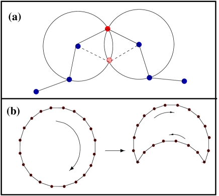
Figure 3: A schematic representation of the Monte Carlo moves: (a) single flip; and (b) global flip.

The algorithm for the Monte Carlo simulation of the discrete model consists of two basic movesKoniaris (1994); van Rensurg et al. (1990): a single particle flip and a global flip. In the single particle flip, a particle is picked at random and reflected about the straight line joining its two neighbours (see Fig. 3(a)). The move is accepted using the standard Metropolis algorithm. Since the energy computation involves only nearby sites, the move is efficient and fast. In the global flip, two particles of the ring are chosen at random and the section of the ring between them is reflected about the line joining the two particles (see Fig. 3(b)). The energy calculation now involves $O(N)$ particles and is thus computationally expensive. However, the global move is crucial to the study of the case where $J\neq 0$, since single particle moves alone are insufficient for equilibration in this case.

In the simulations, one Monte Carlo step is defined as one global move and $N$ single particle moves made by selecting at random particles to be updated. This step is then repeated until the system equilibrates. Thermodynamic quantities are measured from averages taken over independent configurations in equilibrium.

The initial configuration was chosen to be a regular N-sided polygon, but we verified that random configurations also gave the same results. We performed Monte Carlo simulations across a range of pressures for different values of J and system size. The system size varied from $N=64$ to $N=2000$. Typically each parameter value was run for $4\times 10^{6}$ Monte Carlo steps. We waited typically for $10^{6}$ steps for equilibration, averaging data over the remaining steps using independent configurations.

III.2 Exact enumeration

We first describe the algorithm for the case $J=0$. Consider a random walk starting from the origin and taking steps in one of the four possible directions. For each step in the positive (negative) $x$-direction, we assign a weight $e^{-Py}$ ($e^{Py}$), where $y$ is the ordinate of the walker. Multiplying these weights, it is easy to check that the weight is $e^{PA}$ for a closed walk enclosing an area $A$.

Let $T_{N}(x,y)$ be the weighted sum of all $N$-step walks from $(0,0)$ to $(x,y)$. It then obeys the recursion relation,

$$T_{N+1}(x,y) = e^{-Py}T_{N}(x-1,y)+e^{Py}T_{N}(x+1,y)$$ (8)

$$+T_{N}(x,y-1)+T_{N}(x,y+1),$$

with the initial condition

$$T_{0}(x,y)=\delta_{x,0}\delta_{y,0}.$$ (9)

Finally, $T_{N}(0,0)$ gives the partition function of the ring polymer on a lattice.

For the semiflexible case, the recursion relation given above must be modified, since the ring is no longer a simple random walk but a walk with a one step memory. We convert it into a Markov process as follows. Let $T_{N}(x,y;x^{\prime},y^{\prime})$ be the sum of weights of all walks reaching $(x,y)$ in $N$ steps but having been at $(x^{\prime},y^{\prime})$ at the previous step. These $T_{N}$’s are now a Markov process and depend only on $T_{N-1}$’s. The recursion relations are then straightforward to write down. Rather than give all the recursion relations, we provide a representative example

$$T_{N+1}(x,y;x-1,y) = e^{-Py}\big{[}T_{N}(x-1,y;x-2,y)+e^{2J}T_{N}(x-1,y;x,y)$$ (10)

$$+e^{J}T_{N}(x-1,y,x-1,y+1)+e^{J}T_{N}(x-1,y;x-1,y-1)\big{]}.$$

Similar recursion relations will hold for $T_{N+1}(x,y;x+1,y)$, $T_{N+1}(x,y;x,y-1)$ and $T_{N+1}(x,y;x,y+1)$.

The partition function for the polymer problem can be expressed as a sum over areas and bends consistent with a given value of the area, i.e.,

$$\mathcal{Z}_{N}=T_{N}(0,0)=\sum_{A,B}C_{N}(A,B)e^{pA+JB},$$ (11)

where $C_{N}(A,B)$ counts the number of closed paths of area $A$ in a walk of length N which have $B$ bends.

We count up to $N=150$ for different values of $J$. The only limiting factor in going to larger $N$ values is computer memory.

IV Flory-type Scaling Analysis

Flory type scaling theory provides a useful tool to capture the scaling behaviour of systems whose free energy reflects a competition between two or more terms. Such a scaling theory was proposed for the ISIR model in Ref. Haleva and Diamant (2006). A transition from a collapsed to an inflated state was predicted to occur at a critical value of the pressure, whose magnitude scaled with system size as $N^{-1}$. We show how these arguments may be extended to the semiflexible case, deriving expressions for the change in the critical point and scaling as a function of the bending rigidity.

The free energy consists of three terms describing (i) the entropy of the ring, (ii) the pressure differential and (iii) inextensibility of the bonds. When $J=0$, these terms were argued to be $R^{2}/N$, $-PR^{2}$ and $R^{4}/(4N^{3})$ for a ring of size $R$ Haleva and Diamant (2006), where for the second term it was assumed that the area $\langle A\rangle$ scales as $R^{2}$. With semiflexibility, we show that a similar scaling form holds except for $J$ dependent prefactors. Thus, the free energy takes the form

$$F = F_{entropic}+F_{pressure}+F_{inextensibility},$$ (12)

$$\sim \frac{4\pi R^{2}}{N}\left[\alpha(J)-\hat{p}\right]+\frac{\beta(J)R^{4}}{N^{3}}.$$

where we have defined $\hat{p}=Np/4\pi$, and $\alpha$ and $\beta$ depend on $J$.

It is easily seen that a system described by such a Flory theory undergoes a continuous transition when the sign of the $R^{2}/N$ term changes sign. This occurs at a critical scaled pressure $\hat{p}_{c}(J)$ which varies with $J$ as

$$\frac{\hat{p}_{c}(J)}{\hat{p}_{c}(0)}=\frac{\alpha(J)}{\alpha(0)}.$$ (13)

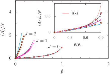
Figure 4: Area versus pressure curves for three $J$ values for $\hat{p}<\hat{p}_{c}$. The points correspond to the discrete case while the lines correspond to the lattice case. The inset shows the collapse when the curves are scaled as in Eq. (14). The $f(x)$ curve in the inset represents the scaling function of Eq. (16). The data is for $N=100$.

When $\hat{p}<\hat{p}_{c}(J)$, then the area follows random walk statistics with $\langle A\rangle\sim N$. In this regime the $R^{4}/N^{3}$ term is not important. For length scales much larger than the persistence length, the problem is effectively one of a freely jointed ring, but with a suitably defined $N$. Thus, we conclude that

$$\langle A(J,N,\hat{p})\rangle=\frac{N}{\hat{p}_{c}(J)}f\left(\frac{\hat{p}}{\hat{p}_{c}(J)}\right),\;\;\;\hat{p}<\hat{p}_{c}$$ (14)

where $f(x)$ is a scaling function. The scaling function $f(x)$ and $\hat{p}_{c}$ can be determined by solving the $J=0$ case (see Appendix A). This gives

$$\hat{p}_{c}=4\pi\alpha(J),$$ (15)

and

$$f(x)=\frac{1}{4\pi x}-\frac{\cot(\pi x)}{4}.$$ (16)

Numerical confirmation of Eqs. (14) and (16) is provided in Fig. 4. The inset shows that the curves for different $J$ collapse onto a single curve when scaled as in Eq. (14).

When $\hat{p}=\hat{p}_{c}$, the scaling is determined by the $R^{4}/N^{3}$ term. Thus, $\langle A\rangle\sim N^{3/2}/\sqrt{\beta(J)}$. Thus,

$$\frac{\langle A(J)\rangle}{\langle A(0)\rangle}=\sqrt{\frac{\beta(0)}{\beta(J)}}.$$ (17)

To test this relation, we compare the Flory prediction with the enumeration results for the area in the lattice model. As can be seen from Fig. 5, there is good agreement for small values of $J$ but the data starts to deviate away from the predicted curve as $J$ increases.

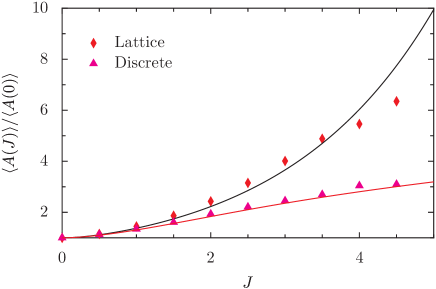
Figure 5: Comparison of the area ratio $\langle A(J)\rangle/\langle A(0)\rangle$ at the critical point with the scaling prediction (see Eqns. (17)) for the lattice (Eq. (32)) and discrete (Eq. (LABEL:betadisc)) models. The scaling prediction is satisfactory for small $J$ but deviates away as $J$ increases.

When $\hat{p}>\hat{p}_{c}(J)$, the ring is in an inflated state, with the area $\langle A\rangle\sim N^{2}$. To obtain an accurate description of this regime, we would need to keep higher order terms such as $R^{6}/N^{5}$ and so on. One thus expects that the lattice and the discrete problems should differ considerably in this regime.

We now derive expressions for $\alpha(J)$ and $\beta(J)$ in both the discrete and lattice cases. This is done by considering a semiflexible chain subjected to an external force. We obtain a perturbative solution for the partition function in the limit of small forces. From the partition function, we obtain the free energy of the ring. By comparing this with the form of Eq. (12), the values of $\alpha(J)$ and $\beta(J)$ can be obtained.

IV.1 Discrete Case

Consider a semiflexible chain of N monomers. When the chain is pulled by a force $\vec{f}$, the partition function is given by

$$Z(J,\vec{f},N)=\int\prod_{j=1}^{N}d\hat{t}_{j}\;e^{J\hat{t}_{j}\cdot\hat{t}_{j+1}}\;e^{\vec{f}\cdot\hat{t}_{j}}.$$ (18)

We work in the limit of small forces, treating the $J$ term exactly. We consider the $f$ term as a perturbation on the zeroth order partition function [ $f=0$ in Eq. (18)], given by

$$Z_{0}(J,N)=[2\pi I_{0}(J)]^{N},$$ (19)

where $I_{0}(J)$ is the modified Bessel function of the first kind of order $0$. We then expand $\exp\left(\sum_{j=1}^{N}\vec{f}.\hat{t}_{j}\right)$ as a series in $f$ and average each term with respect to the zeroth order Hamiltonian. On computing the averages, the partition function is obtained as

$$\ln Z(J,f,N)=\ln Z_{0}+Nb_{2}f^{2}+Nb_{4}f^{4}+O(f^{6}),$$ (20)

where the coefficients $b_{2}$ and $b_{4}$ are given by

$$b_{2} = \frac{I_{0}+I_{1}}{4(I_{0}-I_{1})},$$ (21)

$$b_{4} = \frac{b_{2}^{2}}{4}\left[\frac{2I_{2}}{I_{0}-I_{2}}-\frac{I_{0}+3I_{1}}{I_{0}-I_{1}}\right].$$ (22)

The $I_{n}$’s are modified Bessel functions of the first kind. Their $J$ dependence has been suppressed in the equation above.

The mean end-to-end distance in the limit of small force is obtained from $R\sim\partial\ln Z/\partial f$:

$$\frac{R}{N}=2b_{2}f+4b_{4}f^{3}+O(f^{5}).$$ (23)

Solving for $f$ from Eq. (23), we obtain

$$f=\frac{1}{2b_{2}}\frac{R}{N}-\frac{b_{4}}{4b_{2}^{4}}\left(\frac{R}{N}\right)^{3}+O\left(\left(\frac{R}{N}\right)^{5}\right).$$ (24)

The Flory free energy $F(R)=-\ln Z+fR$, then reduces to

$$F(R)=-\ln Z_{0}+\frac{1}{4b_{2}}\frac{R^{2}}{N}-\frac{b_{4}}{16b_{2}^{4}}\frac{R^{4}}{N^{3}}-pR^{2}.$$ (25)

Comparing with Eq. (12), the factors $\alpha(J)$ and $\beta(J)$ are obtained as

$$\alpha(J) = \frac{1}{4\pi}\frac{I_{0}-I_{1}}{I_{0}+I_{1}}\stackrel{{\scriptstyle J\rightarrow\infty}}{{\longrightarrow}}\frac{1}{16\pi J},$$ (26)

$$\beta(J) = 4\pi^{2}\alpha(J)^{2}\left[\frac{I_{0}+3I_{1}}{I_{0}-I_{1}}-\frac{2I_{2}}{I_{0}-I_{2}}\right]\stackrel{{\scriptstyle J\rightarrow\infty}}{{\longrightarrow}}\frac{7}{64J}.$$

IV.2 Lattice Case

For a lattice polygon, where each individual step can point only in four directions, we solve the problem of a semiflexible chain subject to an external force using the exact $4\times 4$ transfer matrix. The transfer matrix in this case is given by

$$T=\left(\begin{array}[]{llll}e^{J+f}&e^{f/2}&e^{-J}&e^{f/2}\\ e^{f/2}&e^{J}&e^{-f/2}&e^{-J}\\ e^{-J}&e^{-f/2}&e^{J-f}&e^{-f/2}\\ e^{f/2}&e^{-J}&e^{-f/2}&e^{J}\end{array}\right)$$ (28)

We determine the largest eigenvalue up to order $f^{4}$, and hence calculate the partition function:

$$\ln Z(J,f,N) = N\left[\ln(2+e^{-J}+e^{J})+\frac{e^{J}}{4}f^{2}\right.$$ (29)

$$+\left.\frac{1}{192}(e^{J}-3e^{3J})f^{4}+O(f^{6})\right].$$

We then follow the same procedure as for the discrete case, finding $R/N$ in terms of $f$, inverting this equation to find $f$, and finally using this expression to compute the free energy. We thus obtain

$$F(R)=e^{-J}\frac{R^{2}}{N}+\left[\frac{1}{12}e^{-3J}(3e^{2J}-1)\right]\frac{R^{4}}{N^{3}}.$$ (30)

The expressions for $\alpha(J)$ and $\beta(J)$ are then

$$\alpha(J) = \frac{1}{4\pi}e^{-J},$$ (31)

$$\beta(J) = \frac{1}{12}e^{-3J}(3e^{2J}-1).$$ (32)

V Mean Field Theory

In this section we present mean-field theories to calculate the dependence of area on pressure and bending rigidity. In Sec. V.1, we address the ISIR model ($J=0$). The mean field theory presented in Haleva and Diamant (2006) performs poorly with respect to the Monte Carlo data when $\hat{p}>\hat{p}_{c}$. Here, we present an improved variational mean field which reproduces the behaviour of the area above the transition very accurately. It also yields the correct asymptotic behaviour for the area in the limit of high pressures. In this approach, the constraint of fixed link length in treated exactly while the closure constraint is satisfied in a mean field sense. However, such a mean-field theory fails to describe the collapsed phase, also yielding incorrect results for the case of nonzero $J$.

In Sec. V.2, we generalise an earlier mean field theory for the freely jointed chain to include semi-flexibility, imposing the constraint of fixed bond length via a Lagrange multiplier Gaspari et al. (1993); Haleva and Diamant (2006). The closure condition is imposed exactly. We thus derive expressions for the average area of the ring for all pressures and bending rigidity.

V.1 Density matrix mean-field for flexible polymers

In variational theory, a trial density matrix $\rho$ is chosen to approximate the actual density matrixChaikin and Lubensky (1995). The variational parameters are determined by minimising the variational free energy $F_{\rho}$ with respect to the parameters. The simplest mean-field theories assume a trial density matrix that is a product of independent single particle matrices, i.e,

$$\rho=\prod_{j}\rho_{j},$$ (33)

where $\rho_{j}$ is the single particle density matrix of particle $j$. The variational mean-field free energy is

$$F_{\rho}=\langle\mathcal{H}\rangle_{\rho}+T\sum_{j}Tr\rho_{j}\ln\rho_{j}.$$ (34)

The variational form for the density matrix should satisfy the constraint $\rm{Tr}~{}\rho_{j}=1$.

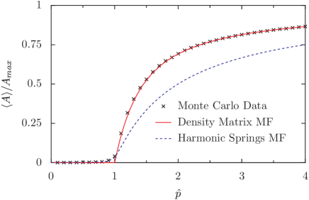
Figure 6: Comparison of Monte Carlo data with the two meanfields for the flexible ($J=0$) case. The density matrix-based mean-field approach provides an accurate description of the area for $\hat{p}>\hat{p}_{c}$.

We choose the single particle density matrix based on the high pressure limit. In this limit, the ground state of our Hamiltonian is a regular N-gon, where the angle of the $j^{th}$ tangent vector is $\theta_{j}=2\pi j/N$. The single particle density matrix has a delta function peak at this value. At intermediate pressures, we therefore take the form of the density matrix to be a gaussian of width $\sigma$ (the variational parameter) centered about $\theta_{j}$:

$$\rho_{j}(\theta_{j})=\frac{1}{\sqrt{2\pi}\sigma\operatorname{erf}[\pi/\sqrt{2}\sigma]}\exp\left[\frac{-(\theta_{j}-\frac{2\pi j}{N})^{2}}{2\sigma^{2}}\right],$$ (35)

where the normalisation ensures that $\rm{Tr}~{}\rho_{j}=1$ and $\operatorname{erf}(x)$ is the error function defined as

$$\operatorname{erf}(x)=\frac{2}{\surd\pi}\int_{0}^{x}e^{-t^{2}}\,dt.$$ (36)

Using this form of the density matrix, we obtain

$$\frac{F_{\rho}}{N}=-\frac{p}{4}\cot\left(\frac{\pi}{N}\right)K(\sigma)^{2}+J\cos\left(\frac{2\pi}{N}\right)K(\sigma)^{2}$$ (37)

$$-\frac{1}{2}+\frac{\sqrt{\pi}\exp(\pi^{2}/(2\sigma^{2}))}{\sqrt{2}\sigma\operatorname{erf}[\pi/\sqrt{2}\sigma]}-\ln\left(\!\!\!\sqrt{2\pi}\sigma\operatorname{erf}[\frac{\pi}{\sqrt{2}\sigma}]\right),\quad$$

where

$$K(\sigma)=\frac{\operatorname{erf}[(\pi-\imath\sigma^{2})/\sqrt{2}\sigma]+\operatorname{erf}[(\pi+\imath\sigma^{2})/\sqrt{2}\sigma]}{2\operatorname{erf}[\pi/\sqrt{2}\sigma]e^{\sigma^{2}/2}}.$$ (38)

When $N\gg 1$, the pressure and bending terms in Eq. (37) can be combined, and the problem is equivalent to one of a flexible polymer ($J=0$) with an effective pressure $\hat{p}_{\mathrm{\rm{eff}}}=\hat{p}+J$.

The variational parameter $\sigma$ is chosen to be the $\sigma^{*}$ that minimises $F_{\rho}$ in Eq. (37). This is done numerically. The average area, equal to $-\partial F_{\rho}/\partial p$, is then given by

$$\langle A\rangle=\frac{N}{4}\cot\left(\frac{\pi}{N}\right)K^{2}(\sigma^{*})\stackrel{{\scriptstyle N\rightarrow\infty}}{{\longrightarrow}}\frac{N^{2}}{4\pi}K^{2}(\sigma^{*}).$$ (39)

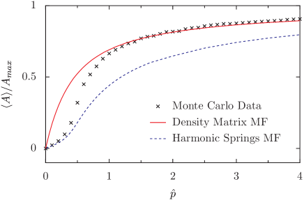
Figure 7: Comparison of Monte Carlo data with the two mean-field approaches for the case $J=1$.

We now derive the asymptotic behaviour of area in the limit of high pressures. We work in the limit when $N$ is large. For large pressures, we expect that $\sigma^{*}$ tends to zero. In this limit

$$K(\sigma)\approx e^{-\sigma^{2}/2},\quad\sigma\rightarrow 0.$$ (40)

and the variational free energy is then given by

$$F_{\rho}(\sigma)=N\left[-(\hat{p}+J)e^{-\sigma^{2}}-\ln(\sqrt{2\pi}\sigma)-\frac{1}{2}\right],$$ (41)

where $\hat{p}=Np/(4\pi)$. Solving $dF_{\rho}/d\sigma^{*}=0$, it is straightforward to obtain

$$\sigma^{*}=\frac{1}{\sqrt{2\hat{p}}}+\frac{1-2J}{4\sqrt{2}\hat{p}^{3/2}},\quad\hat{p}\rightarrow\infty.$$ (42)

The area then reduces to

$$\frac{\langle A\rangle}{N^{2}/4\pi}\rightarrow 1-\frac{1}{2\hat{p}}+\frac{4J-1}{8\hat{p}^{2}},\quad\hat{p}\rightarrow\infty.$$ (43)

For flexible polymers ( $J=0$), this mean-field theory reproduces the $\hat{p}>\hat{p}_{c}$ behaviour very accurately. It also obtains the correct asymptotic behaviour. In Fig. 6, we compare the Monte Carlo data for $J=0$ with the results of the above mean field theory and contrast it with the meanfield theory of Ref. Haleva and Diamant (2006).

The density matrix mean-field however, fails to correctly obtain the behaviour for non-zero values of the bending rigidity. It predicts a first order transition for $J\geq 1$, in disagreement with results from scaling theory. We compare the results of this mean field with the Monte Carlo data in Fig. 7 for a system with $J=1$. This mean-field approach then predicts a transition at $\hat{p}=0$. The discrepancy between the two curves increases for larger values of $J$.

We now describe an alternative mean-field approach to this problem which extends the harmonic spring-based mean field theory of Ref. Haleva and Diamant (2006) to non-zero values of $J$.

V.2 Harmonic spring mean-field for semiflexible polymers

We follow the approach of Refs. Gaspari et al. (1993); Haleva and Diamant (2006) wherein the rigid links between particles are replaced by extensible springs. The spring constant $\lambda$ of the springs is identified with a Lagrange multiplier, chosen so that the mean length of a spring equals unity.

Consider a partition function for N particles given by,

$$\mathcal{Z}\!=\!\!\!\int\!\!d\vec{t}_{j}\exp\!\!\left[\frac{p}{2}\sum_{k<j}\vec{t}_{k}\times\vec{t}_{j}+J\sum_{j}\hat{t}_{j}\cdot\hat{t}_{j+1}\!-\!\lambda\sum_{j}\vec{t}_{j}^{2}\right].$$ (44)

Note that while pressure couples to $\vec{t}$, the bending rigidity couples to the unit vectors $\hat{t}$. We make the approximation of replacing $\hat{t}$ by $\vec{t}$. This makes the problem analytically tractable.

Expanding the tangent vectors in Fourier space as,

$$\hat{t}_{j}^{x} = \sqrt{\frac{2}{N}}\sum_{k}[A_{k}\cos(jk)+B_{k}\sin(jk)],$$

$$\hat{t}_{j}^{y} = \sqrt{\frac{2}{N}}\sum_{k}[A_{k}^{{}^{\prime}}\cos(jk)+B_{k}^{{}^{\prime}}\sin(jk)],$$ (45)

where $k=2\pi l/N$, $l=1,2,\cdots,N$. The partition function then reduces to

$$\mathcal{Z}=\prod_{k}\int dA_{k}dA_{k}^{{}^{\prime}}dB_{k}dB_{k}^{{}^{\prime}}$$ (46)

$$e^{-(\lambda-J\cos k)(A_{k}^{2}+B_{k}^{2}+{A_{k}^{{}^{\prime}}}^{2}+{B_{k}^{{}^{\prime}}}^{2})}e^{\frac{p}{k}(B_{k}A_{k}^{{}^{\prime}}-A_{k}B_{k}^{{}^{\prime}})}.$$

By completing the squares, this integral can be written as a gaussian integral and hence can be calculated exactly. This gives

$$\mathcal{Z}=\prod_{k}\frac{1}{\lambda-J\cos k}\times\left[1-\frac{p^{2}}{4k^{2}(\lambda-J\cos k)^{2}}\right]^{2}.$$ (47)

The parameter $\lambda^{*}$ is determined by equating the mean square link length to one, i.e

$$-\frac{1}{N}\frac{\partial\ln\mathcal{Z}}{\partial\lambda}=1.$$ (48)

This gives

$$N=\sum_{l=1}^{N}\frac{1}{\lambda^{*}-J\cos(\frac{2\pi l}{N})}\left[1\!+\!\frac{2\hat{p}^{2}}{l^{2}[\lambda^{*}-J\cos(\frac{2\pi l}{N})]^{2}\!-\!\hat{p}^{2}}\right],$$ (49)

where $\hat{p}=pN/4\pi$.

When $J=0$, the first factor in Eq. (49) becomes independent of $l$, and then the resultant expression can be evaluated exactly. Hence, an analytic expression for $\lambda^{*}$ can be obtained in this case Haleva and Diamant (2006). For $J\neq 0$, this is no longer possible, and for finite system sizes the resultant equation must be solved numerically. When $N\gg 1$, it is still possible to extract the behaviour of the system analytically.

We now determine the phase boundary from Eq. (49). We will consider the limit $N\gg 1$. First, note that $\lambda^{*}-J\cos(2\pi l/N)\neq 0$ for all $l$. For positive $\lambda^{*}$, this gives the condition that $\lambda^{*}>J$. Second, consider the term in the denominator for $l=1$. It is $(\lambda^{*}-J)^{2}-\hat{p}^{2}$. If we assume that $\lambda^{*}$ is continuous in $\hat{p}$, we have the second constraint that $\lambda^{*}>J+\hat{p}$.

Setting $x=\frac{l}{N}$ and converting the first sum in Eq. (49) to an integral, the equation for $\lambda^{*}$ reduces to

$$1=\frac{1}{\sqrt{\lambda^{*2}-J^{2}}}-\frac{1}{N(\lambda^{*}-J)}$$ (50)

$$+\frac{2}{N(\lambda^{*}-J)}\sum_{k=1}^{\infty}\left(\frac{\hat{p}}{\lambda^{*}-J}\right)^{2k}\!\!\frac{1}{2k-1}+\mathcal{O}(\frac{1}{N^{2}}).\quad$$

The sum in Eq. (50) is convergent if the ratio $\hat{p}/(\lambda^{*}-J)<1$. In this case, we keep only the first term on the right hand side of Eq. (50). This gives,

$$\lambda^{*}=\sqrt{1+J^{2}},\;\;\;\mathrm{for}\;\hat{p}<\hat{p}_{c}.$$ (51)

The critical pressure is obtained when the ratio $\hat{p}/(\lambda^{*}-J)$ becomes equal to $1$, i.e.

$$\hat{p}_{c}(J)=\lambda^{*}-J=\sqrt{1+J^{2}}-J.$$ (52)

For large values of $J$, this goes as $\hat{p}_{c}(J)\sim 1/2J$, which differs by a factor of $2$ from the answer obtained by scaling arguments [see Eq. (26)].

We shall now estimate $\lambda^{*}$ in the different scaling regimes. We assume that $\lambda^{*}$ is a non-decreasing function of $\hat{p}$ (as in $J=0$). Then, since we have the constraint of $\lambda^{*}>\hat{p}+J$, the ratio $\hat{p}/(\lambda^{*}-J)$ must continue to remain at $1$ for $\hat{p}>\hat{p}_{c}$. Thus, above the critical point, we obtain

$$\lambda^{*}=\hat{p}+J,\;\;\;\mathrm{for}\;\hat{p}>\hat{p}_{c}.$$ (53)

However, a simple substitution of Eq. (53) in Eq. (49) for $\hat{p}>\hat{p}_{c}$ does not satisfy Eq. (49). We therefore need to calculate the correction term arising from large but finite $N$. We start by considering Eq. (49). The first term can be summed exactly, giving

$$N\left(1-\frac{1}{\sqrt{\lambda^{2}-J^{2}}}\right)$$ (54)

$$=\sum_{l=1}^{N}\frac{1}{\lambda-J\cos(\frac{2\pi l}{N})}\frac{2\hat{p}^{2}}{l^{2}(\lambda-J\cos(\frac{2\pi l}{N}))^{2}-\hat{p}^{2}}.$$

We calculate the finite size corrections to $\lambda^{*}$ as follows. Let

$$\lambda^{*}_{\hat{p}\geq\hat{p}_{c}}=\hat{p}+J-\delta.$$ (55)

When $\delta\rightarrow 0$, the main contribution to the left hand side of Eq. (54) comes from the $l=1$ term. The contribution from other $l$ is convergent as $\delta\rightarrow 0$. Expanding the right hand side as a series in $\delta$, we obtain

$$-\frac{1}{\delta}=N\left[1-\frac{1}{\sqrt{\hat{p}^{2}+2\hat{p}J}}-\frac{\delta(\hat{p}+J)}{(\hat{p}^{2}+2\hat{p}J)^{3/2}}\right].$$ (56)

The $\delta$ independent term in the right hand side of Eq. (56) is nonzero for $\hat{p}>\hat{p}_{c}$ and is equal to zero for $\hat{p}=\hat{p}_{c}$. Thus, when $\hat{p}>\hat{p}_{c}$, we keep only the first term in the right side, while at $\hat{p}=\hat{p}_{c}$, we need to keep the second term too. Solving for $\delta$, we obtain,

$$\delta=\begin{cases}\frac{1}{\sqrt{N}}\frac{1}{(1+J^{2})^{1/4}},&\text{ $\hat{p}=\hat{p}_{c}$,}\\ \frac{1}{N}\frac{\sqrt{\hat{p}^{2}+2\hat{p}J}}{\sqrt{\hat{p}^{2}+2\hat{p}J}-1},&\text{ $\hat{p}>\hat{p}_{c}$.}\end{cases}$$ (57)

We are now in a position to calculate the mean area $\langle A\rangle$ from $\frac{\partial\ln\mathcal{Z}}{\partial p}$. This gives,

$$\langle A\rangle=\frac{N\hat{p}}{2\pi}\sum_{l=1}^{N}\frac{1}{l^{2}(\lambda^{*}-J\cos(\frac{2\pi l}{N}))^{2}-\hat{p}^{2}}.$$ (58)

The numerical values obtained for $\lambda$ are then substituted in this equation to get the corresponding value of the area. We can, however, analytically determine the scaling behaviour of the area in the limit of large system sizes from the values of $\lambda$ calculated above.

For $\hat{p}<\hat{p}_{c}$, we have,

$$\langle A\rangle\simeq\frac{N\hat{p}}{2\pi}\sum_{l=1}^{N}\frac{1}{l^{2}(\sqrt{1+J^{2}}-J\cos(2\pi l/N))^{2}-\hat{p}^{2}}$$ (59)

At the critical point, we obtain, from Eqns. (56) and (58),

$$\langle A\rangle=N^{3/2}\frac{(1+J^{2})^{1/4}}{4\pi},\quad\hat{p}=\hat{p}_{c}.$$ (60)

Similarly, for pressures greater than the critical pressure, we obtain, from Eqns. (53) and (58),

$$\langle A\rangle=\frac{N^{2}}{4\pi}\left[1-\frac{1}{\sqrt{\hat{p}^{2}+2\hat{p}J}}\right]\stackrel{{\scriptstyle\hat{p}\rightarrow\infty}}{{\longrightarrow}}\frac{1}{\hat{p}}-\frac{J}{2\hat{p}^{2}},~{}\hat{p}>\hat{p}_{c}.$$ (61)

This mean field theory reproduces the qualitative behaviour of the simulation data correctly. It predicts a continuous transition for all $J$, unlike the density matrix field theory. However, there is a quantitative disagreement with the data. This can be seen by comparing the results of this mean-field theory with the simulation data in both the flexible (Fig. 6) and semi-flexible (Fig. 7) polymer cases.

VI Scaling and Critical Exponents

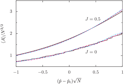
Figure 8: Area collapse for flexible and semiflexible polymers around the critical point. This verifies Eq. (62). The data is for $N=80,100,120,140,150$ for the lattice problem.

The order parameter that describes the collapsed to inflated phase transition is the ratio of the area to the maximum area. When $N\gg 1$, the ratio is zero below the transition and non-zero above it. The behaviour near the transition line can be described by the scaling form

$$\frac{\langle A\rangle}{A_{max}}\simeq N^{-\phi\beta}g\left[(\hat{p}-\hat{p}_{c})N^{\phi}\right],$$ (62)

where $\phi,\beta$ are exponents and $g(x)$ is a scaling function. When $x\rightarrow 0$, then $g(x)\rightarrow\rm{constant}$. When $x\rightarrow\infty$, then $g(x)\sim x^{\beta}$. When $x\rightarrow-\infty$, then $g(x)\sim 1/x$ [see Eqs. (14) and (16)]. This immediately implies that

$$\phi(1+\beta)=1.$$ (63)

To obtain the one independent exponent, we resort to the scaling theory (see Sec. IV). At $\hat{p}_{c}$, $\langle A\rangle/A_{\rm{max}}\sim 1/\sqrt{N}$. At the critical point, the area scales as $N^{3/2}$. Combing with Eq. (63), we obtain $\phi=1/2$ and $\beta=1$. These exponents are independent of $J$.

In Fig. 8, we show scaling plots when area is scaled as in Eq. (62) with $\phi$ and $\beta$ as above for the cases $J=0$ and $J=0.5$. The excellent collapse shows that the Flory type scaling theory gives the correct exponents.

We now look at the fluctuations. Consider the compressibility $\chi$ defined as

$$\chi=\frac{1}{A_{\rm{max}}}\frac{\partial\langle A\rangle}{\partial p}.$$ (64)

When $\hat{p}<\hat{p}_{c}$, $\chi$ can be calculated from Eqs. (14) and (16) to be

$$\chi=-\frac{1}{\hat{p}^{2}}+\frac{\pi^{2}}{\hat{p}_{c}^{2}\sin^{2}(\pi\hat{p}/\hat{p}_{c})},~{}~{}\hat{p}<\hat{p}_{c}.$$ (65)

Thus, $\chi$ diverges as $(\hat{p}_{c}-\hat{p})^{-2}$ below the transition point. The behaviour near the transition point is described by the scaling form

$$\chi\simeq N^{\phi\gamma}h\left[(\hat{p}-\hat{p}_{c})N^{\phi}\right],$$ (66)

where $h(x)$ is a scaling function and $\phi=1/2$. When $x\rightarrow 0$, then $h(x)\rightarrow\rm{constant}$. When $|x|\gg 1$, then $h(x)\sim x^{-\gamma}$. Comparison with Eq. (65) gives $\gamma=2$.

In Fig. 9, we plot the compressibility scaled as in Eq. (66) for two different values of $J$. A good collapse is obtained again showing that the Flory type scaling theory gives the correct exponents. Similar, but noisier data can be obtained for the discrete model. We thus conclude that the introduction of semiflexibility does not affect any of the exponents describing the transition.

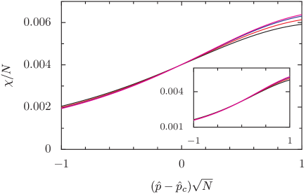
Figure 9: The scaling plots for compressibility $\chi$ when scaled as in Eq. (66). The data is for the lattice model with $J=0.5$ and $J=0$ (inset). The system sizes are $N=80,100,120,140,150$.

VII The lattice problem

In this section, we present some additional enumeration results for the lattice problem. Consider the scaling theory presented in Sec. IV. The inextensibility of the polymer was captured by the $R^{4}/N^{3}$ term for a polymer of extent $R$. This was obtained from a calculation based on the extension of a polymer under a force. Here we present numerical evidence supporting this.

Let $P_{N}(A)$ be the probability (at $P=0$) that a walk of length $N$ encloses an area $A$. In Appendix A, we show that [see Eq. (78)]

$$P_{N}(A)=\frac{1}{N}I\left(\frac{A}{N}\right),~{}A,N\rightarrow\infty,~{}\frac{A}{N}~{}\rm{fixed}.$$ (67)

where the scaling function $I(x)$ is given by

$$I(x)=\pi~{}\mathrm{sech}^{2}(2\pi x).$$ (68)

We consider the corrections to the scaling form in Eq. (67). Let

$$E_{N}(A)=\frac{NP_{N}(A)}{I(A/N)}.$$ (69)

Scaling theory predicts that $E_{N}(A)$ should be a function of one variable $A^{2}/N^{3}$. This is verified in Fig. 10 where $\ln E_{N}(A)$ is plotted against $A^{2}/N^{3}$ for a range of system sizes.

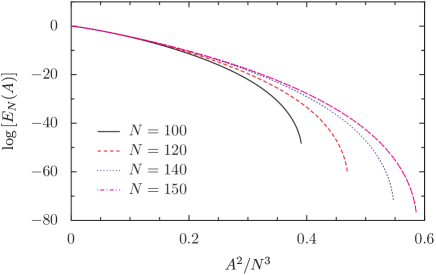
Figure 10: Collapse of the $E_{N}(A)$ for different values of $N$ when plotted against $A^{2}/N^{3}$. The data is for the lattice model with $J=0$.

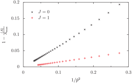
Figure 11: The asymptotic behaviour of area in the limit of large $\hat{p}$ as computed for the lattice model. The curves are straight lines when plotted against $1/\hat{p}^{2}$.

We also study the behaviour of area when $\hat{p}$ is very large. When $\hat{p}\gg 1$, the behaviour is seen to differ from the discrete version of the problem. It can be shown to beMitra et al.

$$1-\frac{\langle A\rangle}{A_{\rm{max}}}\sim\frac{1}{\hat{p}^{2}},\quad\hat{p}\rightarrow\infty.$$ (70)

This should be contrasted with the discrete case which varied as $1/\hat{p}$. In Fig. 11, we show numerical confirmation of the prediction of Eq. (70).

VIII Conclusions

In this paper, we have proposed and studied lattice and discrete models for self-intersecting pressurised semi-flexible polymers. Our work generalises results of Ref. Haleva and Diamant (2006) to include a bending rigidity. A simple variational mean-field approach provides very accurate fits to the Monte Carlo data for this problem in the absence of semi-flexibility. The mean-field approach for $J=0$ Rudnick and Gaspari (1991); Gaspari et al. (1993); Haleva and Diamant (2006) was generalised to the semiflexible case. The phase boundary between collapsed and inflated phases as well as expressions for the area as a function of $p$ and $J$ in the different phases were obtained analytically.

We have shown that the essence of the physics is captured through simple Flory approximations. The scaling predictions of the Flory theory were verified numerically for both the lattice and discrete cases.

We have also investigated the behaviour of the system in the extreme limits of a fully pressurised polymer ring and a collapsed configuration. For the fully pressurised ring, we deduce the leading order asymptotic behaviour of the area in both the discrete and lattice cases. The collapsed phase was studied by mapping this problem onto a quantum mechanical problem of an electron confined to two dimensions and placed in a transverse magnetic field. The analytic results thus obtained fit the data accurately.

The usefulness of these results for more realistic systems lies in the fact that both the restriction to the signed area as well as allowing for self-intersections at no energy cost are irrelevant in the large $p$ limit. The results obtained at large $p$ should therefore apply both qualitatively and quantitatively to the more realistic case of a pressurised self-avoiding polymer, where the pressure term couples to the true physical area and not to the signed area. This is the LSF model Leibler et al. (1987). The approach presented here is thus also useful in understanding the behaviour of a larger class of models, some of which are more physical in character, but which lack the analytic tractability of the model proposed and studied here.

Appendix A Analytic answer in the small pressure regime

The problem of self-intersecting polymers in two dimensions with no bending rigidity ($J=0$) is analogous to the quantum mechanical problem of an electron moving in a magnetic field applied transverse to the plane of motion. Using this analogy, we obtain analytic expressions for the partition function $\mathcal{Z}$ and $C_{N}(A)$, the number of closed walks of area $A$.

When an electron goes around a magnetic field, it picks up a phase factor proportional to the flux enclosed by the path. This flux is proportional to the product of the strength of the magnetic field times the algebraic area enclosed by the loop. The propagator then is the sum over all such loops. This suggests that the partition function for the polymer problem can be obtained from the quantum mechanical propagator for the electron problem provided the constants are appropriately mapped.

For an electron of charge $e$ and mass $m$ in a constant external magnetic field $B$, in the z direction, in the case when the electron returns to the origin, the kernel can be written as Feynman and Hibbs (1965),

$$K(0,0;t,0)=\left(\frac{m}{2\pi i\hbar t}\right)\left(\frac{\omega t/2}{\sin\omega t/2}\right),$$ (71)

where $\omega=eB/mc$. It picks up a flux $\Phi$ given by

$$\Phi=\frac{eBA}{\hbar c}.$$ (72)

The motion of a quantum mechanical particle is governed by the two-dimensional Schroedinger equation,

$$\imath\hbar\frac{\partial\psi}{\partial t}=\frac{-\hbar^{2}}{2m}\left(\frac{\partial^{2}\psi}{\partial x^{2}}+\frac{\partial^{2}\psi}{\partial y^{2}}\right).$$ (73)

The classical diffusion equation for a particle in two-dimensions is

$$\frac{\partial P}{\partial t}=\frac{1}{4}\left(\frac{\partial^{2}P}{\partial x^{2}}+\frac{\partial^{2}P}{\partial y^{2}}\right),$$ (74)

where $P(x,y)$ is the probability of finding the particle at $(x,y)$. Thus to map the results of the quantum problem onto the polymer problem, we need to map $t\rightarrow-it$ and also identify

$$\frac{\hbar}{2m}=\frac{1}{4}.$$ (75)

Also, to match the diffusion constant, we need,

$$\frac{\imath eB}{\hbar c}=p.$$ (76)

Substituting in the propagator and equating it to the partition function, we obtain

$$\mathcal{Z}=\frac{4^{N}}{4\pi}\frac{p}{\sin\frac{pN}{4}}.$$ (77)

where we have introduced the appropriate normalisation factors. $C_{N}(A)$ is now obtained from the partition function by performing the inverse Laplace Transform with respect to $p$. This gives

$$C_{N}(A)=\frac{4^{N+1}}{2N^{2}}\mathrm{sech}^{2}\frac{2\pi A}{N}.$$ (78)

and

$$\langle A\rangle=\frac{1}{p}-\frac{N}{4}\cot\left(\frac{Np}{4}\right).$$ (79)

The free energy will have a singularity at $p=4\pi/N$. Below this $p$, the expressions are valid for both the discrete case and the lattice. Exactly the same expression has been obtained by using the harmonic spring approximation Rudnick and Gaspari (1991). The expression for area matches both the simulation and lattice data quite closely for low pressures, as can be seen from Fig. 4.

Moreover, if we recall the Flory prediction that by rescaling area and pressure by $\hat{p}_{c}(J)$, we can obtain the results for non-zero values of the bending rigidity from the answer of the problem with $J=0$, we see that the above analysis also predicts the area expression for nonzero values of $J$.

References

- Canham (1970) P. Canham, J. Theor. Biol. 26, 61 (1970).
- Helfrich (1973) W. Helfrich, Z. Naturforsch. 28, 693 (1973).
- Evans (1974) E. Evans, Biophys. J. 14, 923 (1974).
- Seifert (1997) U. Seifert, Adv. Phys. 46, 13 (1997).
- Leibler et al. (1987) S. Leibler, R. R. P. Singh, and M. E. Fisher, Phys. Rev. Lett. 59, 1989 (1987).
- Fisher (1989) M. E. Fisher, Physica D 38, 112 (1989).
- Camacho and Fisher (1990) C. J. Camacho and M. E. Fisher, Phys. Rev. Lett. 65, 9 (1990).
- van Rensburg (2000) E. J. J. van Rensburg, The Statistical Mechanics of Interacting Walks, Polygons, Animals and Vesicles (Oxford University Press, 2000).
- Fisher et al. (1991) M. E. Fisher, A. J. Guttmann, and S. G. Whittington, J. Phys. A 24, 3095 (1991).
- Bousquet-Mélou (1996) M. Bousquet-Mélou, Disc. Math. 154, 1 (1996).
- Guttmann and Lin (1992) Articles by A. J. Guttmann and K. Y. Lin, in AIP Conference Proceedings, edited by C. K. Hu (1992), vol. 248.
- Richard et al. (2001) C. Richard, A. J. Guttmann, and I. Jensen, J. Phys. A 34, L495 (2001).
- Cardy (2001) J. Cardy, J. Phys. A 34, L665 (2001).
- Richard (2002) C. Richard, J. Stat. Phys. 108, 459 (2002).
- Richard et al. (2003) C. Richard, I. Jensen, and A. J. Guttmann, Proceedings of the International Congress on Theoretical Physics TH2002 (Paris) pp. 267–277 (2003).
- Rajesh and Dhar (2005) R. Rajesh and D. Dhar, Phys. Rev. E 71, 016130 (2005).
- Rudnick and Gaspari (1991) J. Rudnick and G. Gaspari, Science 252, 422 (1991).
- Gaspari et al. (1993) G. Gaspari, J. Rudnick, and A. Beldjenna, J. Phys. A 26, 1 (1993).
- Marconi and Maritan (1993) U. M. B. Marconi and A. Maritan, Phys. Rev. E 47, 3795 (1993).
- Haleva and Diamant (2006) E. Haleva and H. Diamant, Eur. Phys. J. E 19, 461 (2006).
- Koniaris (1994) K. Koniaris, J. Chem. Phys. 101, 731 (1994).
- van Rensurg et al. (1990) E. J. J. van Rensurg, S. Whittington, and N. Madras, J. Phys. A 23, 1589 (1990).
- Chaikin and Lubensky (1995) P. Chaikin and T. Lubensky, Principles of Condensed Matter Physics (Cambridge University Press, 1995).
- (24) M. K. Mitra, G. I. Menon, and R. Rajesh, Inflated self avoiding polygons, unpublished.
- Feynman and Hibbs (1965) R. Feynman and A. Hibbs, Quantum Mechanics and Path Integrals (McGraw-Hill Book Company, 1965).