Autocatalytic reaction on low-dimensional substrates

Abstract

We discuss a model for the autocatalytic reaction $A+B\rightarrow 2A$ on substrates where the reactants perform a compact exploration of the space, i.e., on lattices whose spectral dimension $\tilde{d}$ is $<2$. For finite systems, the total time $\tau$ for the reaction to end scales according to two different regimes, for high and low concentrations of reactants. The functional dependence of $\tau$ on the volume of the substrate and the concentration of reactants is discussed within a mean-field approximation. Possible applications are discussed.

1 Introduction

Diffusion-reaction processes is a long standing problem which finds a number of applications, especially in physics bartumeus , chemistry and biology hess .

Most of the earlier studies focus the attention on a single particle diffusing in the presence of immobile reactants, while much less is known about the statistical properties associated with the diffusion of a set of particles, notwithstanding its interest. Indeed, multiparticle diffusion problems are difficult to manage due to the fact that the effects of each single particle do not combine linearly, even in the noninteracting case yuste . In the last years much effort has been devoted to the formulation of rigorous many-body treatments of diffusion controlled reactions especially in low dimension. In fact, while in high dimensions a mean-field approach provides a good description, in low dimension local fluctuations are responsible for significant deviation from mean-field predictions toussaint .

In general, a great deal of recent experimental as well as theoretical work has been devoted to the study of such diffusion-reaction processes in restricted geometries. The latter expression refers to two different (possibly concurrent) situations: that of a low dimensionality, and that of a small spatial scale. In the first case, the spectral dimension $d$ characterizing the diffusive behavior of the reactants on the substrate is low ($1<d<2$), and the substrate underlying the diffusion-reaction lacks spatial homogeneity. Hence, there are considered media whose properties are not translationally invariant and where the reactants perform a “compact exploration” of the space degennes . These kinds of structures can lead to a chemical behavior significantly different from those occurring on substrates displaying an homogeneous spatial arrangement. This is the case, for example, of fractal lattices: in the last 20 years, an extensive literature has been investigating the consequences of a fractal geometry on the laws of reaction kinetics blumen , for example for the one-species ($A+A\rightarrow\emptyset$)zumofen1 and two-species ($A+B\rightarrow\emptyset$)zumofen1 ; lindenberg ; zumofen2 annihilation reactions. In all these systems the role of the generally noninteger spectral dimension, whose definition will be discussed below, is stressed, as opposed to the integer euclidean dimension characterizing homogeneous structures.

But restricted geometry also refers to a variety of experimental situations in which these processes occur on spatial scales too small to allow an infinite volume treatment. The so-called finite-size corrections to the asymptotic (infinite-volume) behavior in this case become predominant. Indeed, previous works considered infinite systems (both euclidean and fractal), and studied their properties in some kind of thermodynamic limit; typically, sending the volume to infinity while keeping the density of reactants fixed. Therefore, they considered the critical properties of the systems (for example, the scaling of the density of reactants) for $t\rightarrow\infty$, hence, for an infinite time lapse of the reaction. One of the most important issues of this paper regards the finite size of the systems under study. In this work we examine explicitly finite systems where no thermodynamic limit has to be taken. All the quantities we calculate, in particular the total reaction time $\tau$, are hence finite, and we seek their dependence on the finite parameters of the system (volume of the reaction and concentration of the reactants).

In particular, in this paper we study the dynamics of a system made up of two species particles undergoing irreversible quadratic autocatalytic reactions according to the following scheme: $A+B\rightarrow 2A$, with reaction probability set equal to one. All particles move randomly and particles of different kinds react on encounter, i.e. the reaction is strictly local and deterministic. Autocatalytic reactions have been extensively analyzed on Euclidean structures, both analytically and numerically lemarchand ; mai1 ; mai2 ; velikanov ; warren ; chaivorapoj . A continuous picture of this system can be attained by the Fisher equation fisher ; kolmo which describes the system in terms of front propagation; however, this picture will not intervene in our calculations, that will mostly concern the low-density regime, where a front propagation cannot be defined.

While previous works on autocatalytic reactions considered reactions on Euclidean lattices, here we focus, as mentioned above, on low dimensional structures ($1<d<2$), hence considering media whose properties are not translationally invariant. Our investigations are especially concerned with the role of topology in the temporal evolution of the system. In particular, we will consider the concentration $\rho_{A}(t)$ of A particles present in the system at time $t$ and its fluctuations. From $\rho_{A}(t)$ it is also possible to derive an estimate for the reaction velocity. Furthermore, we consider the average time $\tau$ at which the system achieves its inert state, i.e. $N_{A}=N$. We call this time “Final Time”. As we will show, $\tau$ depends on the number of particles $N$ and on the volume $V$ of the underlying structure, meant as the total number of sites. More precisely, it will be shown, both numerically and analytically, that for small concentrations of the reactants the “Final Time” factorizes into two terms depending on $N$ and $V$ respectively. This results agrees with previous works where the model under study was analyzed for Euclidean lattices earlier1 ; earlier2 . We will also show how this dependence could provide a practical tool for the determination of the concentration of reactants, especially when very small concentrations have to be detected endo .

The plan of the paper is the following. In Sec. 2 we introduce the model, we recall previous results on Euclidean substrates (Sec. 2.1) and discuss the main features of inhomogeneous lattices (Sec. 2.2). In Sec. 3 we show our analytical results concerning those lattices; Sec. 4 discusses the results of numerical simulations. Sec. 5 contains our conclusions.

2 The model

We consider a system made up of $N$ particles of two different chemical species $A$ and $B$, diffusing and reacting on a discrete substrate with no excluded volume effects. The volume of the substrate is $V$; at time $t$, $N_{A}(t)$ and $N_{B}(t)$ are the number of $A$ and $B$ particles, respectively, with $N=N_{A}+N_{B}$. We define $\rho_{A}(t)=N_{A}(t)/V$ and $\rho_{B}(t)=N_{B}(t)/V$ as the concentrations of the two species at time $t$.

Different species particles residing at time step $t$, on the same node or on nearest-neighbor nodes react according to the following mechanism:

$$A+B\rightarrow 2A$$

with reaction probability set equal to one, so that the process is strictly diffusion-controlled. Notice that the previous scheme is quite general as it also includes possible additional products (other than $2A$) made up of some inert species of no consequences to the overall kinetics.

The initial condition at time $t=0$ is $N_{A}(0)=1,N_{B}(0)=N-1$, with all particles distributed randomly throughout the substrate. As a consequence of the chemical reaction defined above, $N_{A}(t)$ is a monotonic function of $t$ and, due to the finiteness of the system, it finally reaches value $N$; at that stage the system is chemically inert. The average time at which $N_{A}(t)=N$ is called “Final Time” and denoted by $\tau$.

The Final Time $\tau$ is of great experimental importance since it provides an estimate of the time when reaction-induced effects (such as side-reactions or photoemission) vanish ichimura .

In this perspective, deviations from the theoretical prediction of $\tau$ are, as well, noteworthy: they could reveal the existence of competitive reactions merkin or explain how the process is affected by external radiation singh .

However, one of the most interesting applications of the Final Time is analytic endo ; ishihara : as we will show, $\tau$ sensitively depends on $N$, that is on the initial amount of reactant. Hence, given a trace reactant, its determination can be achieved by means of spectrophotometric measures of $\tau$.

Indeed, our results confirm that this technique can be extremely sensitive endo ; kato and the determination of ultratrace amounts is therefore possible.

We stress again that he following analysis mainly focuses on high-diluted finite-size systems. The experimental applications previously described concerns finite systems; furthermore, we aim to evidence the role of the substrate topology which just emerges in the diffusion-limited regime.

2.1 Euclidean Substrate

The quadratic autocatalytic system for diffusing reactants on Euclidean lattices has been analyzed in detail in earlier works earlier1 ; earlier2 in the context of information spreading. It also provides a simple model for epidemic systems: $A$ ($B$) particles stand for (irreversibly) sick (healthy) or informed (unaware) individuals respectively. For these systems as well a knowledge of the rate of infection or information diffusion is of great importance. We briefly review the results obtained in earlier1 ; earlier2 for $\tau$ on Euclidean lattices.

In general, $\tau$ depends on system parameters $N$ and $L$ and, in the low-concentration regime, and for the Euclidean lattices this dependence can be factorized into two contributions depending on $N$ and $L$ respectively, and whose functional form depends on the dimension of the lattice. A mean-field calculation for $\tau$ provides exact results for $d>2$ and $d=1$, while dimension $d=2$ is marginal. Our previous results can be summarized as follows:

$$\tau(N,L)\sim\ \left\{\begin{array}[]{ccc}\displaystyle C_{1}\frac{L^{2}}{N}&d=1\\ \\ f_{2}(N)\,L^{2}\,\mathrm{ln}(L)&d=2\\ \\ \displaystyle C_{d}\frac{\gamma+\mathrm{ln}(N)}{N}\,L^{d}&d\geq 3,\end{array}\right.$$ (1)

where $C_{d}$ are dimension-depending constants and fitting procedures suggest $f_{2}(N)=\frac{A+ln(N)}{N}$ (for further details see earlier2 ).

2.2 Inhomogeneous Structures

Figure 1: Sierpinski gasket of generation 4: $V=\frac{3}{2}(3^{3}-1)$.

Figure 2: T-fractal of generation 4: $V=3^{4}+1$.

Figure 3: Comb Lattice

A number of problems in physics and chemistry are related to random walks on homogeneous structures. In the last few years there is a growing interest in the theory of diffusion in low and fractal dimensions havlin . In fact, most of the materials existing in nature show a disordered, non-crystalline geometrical structure. Indeed, fractals are good models for disordered systems since they usually display a dilation symmetry which is a fractal characteristic. Apart from the applications point of view, low dimensional systems are of great theoretical importance. As previously underlined, when diffusion is considered, low dimensional structures dramatically affect the kinetic laws.

Fractals are self-similar structures exhibiting dilation symmetry. Differently from Euclidean structures, their description requires at least two (typically noninteger) different dimensions. The first is the fractal dimension $d_{f}$, that gives the dependence of the volume of the system (i.e., the number of sites it contains) on its linear size

$$V(L)\sim L^{d_{f}}.$$

The second is the spectral dimension $\tilde{d}$, which governs (among other phenomena) the long-time properties of diffusion on the lattice. Indeed, if we consider a random walkers starting from a given site $i$ of the lattice, the probability $P_{ii}(t)$ of returning back to the starting point at time $t$, at large times, follows the law

$$P_{ii}(t)\sim t^{-\tilde{d}/2}.$$

Also, the number $S(t)$ of different sites visited by the random walker at time $t$ is for large times:

$$S(t)\sim t^{\tilde{d}/2} \;\mathrm{for}\;\tilde{d}\leq 2$$ (2)

$$S(t)\sim t \;\mathrm{for}\;\tilde{d}>2$$

For $\tilde{d}<2$ the random walker returns to its starting site with probability 1 and the lattice is called recurrent; for $\tilde{d}>2$ the probability of return is less than 1 and the lattice is called transient (lattices with $\tilde{d}=2$ have to be discussed case by case). For $\tilde{d}<2$ the walker is also said to perform a compact exploration of the space degennes , since the (fractal) dimension of the random walk trajectory is greater than the dimension $d_{f}$ of the underlying lattice.

The spectral dimension is of a more general interest than the fractal dimension, since it can also be defined for inhomogeneous structures that lack a dilation invariance, hence for which a fractal dimension $d_{f}$ cannot be defined.

The two fractals we consider in this paper, the Sierpinski gasket and the T-fractal, have both $\tilde{d}<2$.

The Sierpinski gasket is generated by iterating in a recurrent fashion a generating cell consisting of a triangle (Fig.1). The number of iterations is called the generation $g$ of the fractal. The total number of triangles after $g$ iterations is $3^{g}$, while the total number of sites (hereafter called volume $V$) is $V=3\frac{3^{g}+1}{2}.$ The linear size of the gasket is given by $2^{g}$. The Sierpinski gasket has fractal dimension $d_{f}=\frac{\log 3}{\log 2}\approx 1.584$ and spectral dimension $\tilde{d}=\frac{\log 9}{\log 5}\approx 1.365.$

The T-fractal is constructed from a 4-sites T-shaped generating cell (Fig.2). It has fractal dimension $d_{f}=\frac{\log 3}{\log 2}\approx 1.584$ and spectral dimension $\tilde{d}=\frac{\log 9}{\log 6}\approx 1.226.$

The third structure we will consider, the comb lattice (Fig.3), does not present dilation invariance; hence, the $d_{f}$ cannot be defined. As we said above, it is still possible to define a spectral dimension that turns out to be $\tilde{d}=3/2$.

Some linear problems have already been solved exactly on these structures using renormalization groups technique (see for example broek ). However, for many interacting diffusing particles an exact solution is not feasible and we rely mainly on numerical simulations.

3 Analytical Results

In this section we study the irreversible autocatalytic reaction occurring in a close system by means of a mean field approximation. This kind of approach is very different from those previously adopted for this kind of system.

An analytical result for the dependence of the Final Time $\tau$ on $V$ and $N$ is difficult to find: approximate calculations can be carried out in the two limit regimes of high and low concentration.

For high concentration ($\rho\gg 1$) the results found in Euclidean structures earlier1 continue to hold for inhomogeneous geometries: the $A$ particles occupy a connected region of the space for all $t$. The border of this region expands at a fixed velocity, such that at time $t$ the region covers all the sites whose chemical distance from the starting point of the seed particle is $\leq 2\,t$. Hence, for a finite system like those we are considering here, the Final Time is $\tau=l_{\mathrm{max}}/2$, where $l_{\mathrm{max}}$ is the chemical distance of the most distant point on the lattice, starting from the seed particle. On Euclidean geometries this yields $\tau=L/2$ for $d=1$ and $\tau=L$ for $d\geq 2$. On the other hand, on inhomogeneous structures the dependence on $L$ is not so simple, since it involves taking the average with respect to all possible starting points for the seed particle; anyway, the crossover between this high-concentration regime and the low-concentration one remains apparent.

Our mean-field approach is based on a different point of view and the assumptions introduced make it valid just in the low-concentration regime. In this approach we focus on collective quantities lacking the spatial dependence.

In particular our hypothesis is that the time elapsing between a reaction and the successive one is long enough that the spatial distribution of reactants can be considered as uniform. This assumption corresponds to a mean field approach since we neglect correlations between spatial position of reactants; in other words we neglect the fact that for small times after a reaction the two A particles are likely to be find nearby. This kind of hypothesis is therefore valid for small concentration of reactants, i.e. $\rho\ll 1.$ As a consequence of this hypothesis we can just focus on two-body interactions among particles since the event of three or more reactants interacting together is unlikely at small densities.

First of all we consider the final time $\tau$. Let us define $\langle t_{n}\rangle$ the time elapsing between the $n-1$-th first encounter among different particles and the $n$-th one. This time corresponds to the average time during which there are just $N_{A}(t)=n$ particles in the systems. In the mean field approximation this is proportional to the trapping time in the presence of $n$ traps randomly distributed through a volume $V$. For compact exploration of the space ($\tilde{d}<2$) degennes , the average trapping time $t_{\mathrm{trap}}$ for a random walker in a distribution of $N-N_{A}$ randomly distributed moving traps is given by oshanin

$$t_{\mathrm{trap}}\sim\rho_{\mathrm{trap}}^{-2/\tilde{d}}=\left(\frac{V}{N_{A}(t)}\right)^{2/\tilde{d}},$$

since the density of traps is $\rho_{traps}=N_{A}(t)/V$. Here, the symbol $\sim$ denotes proportionality.

This is the trapping time for one particle in a background of moving traps; we are interested in the average trapping time of the first out of $N-N_{A}$ particles, that for rare events is just the same time rescaled by a factor $N-N_{A}$ (the number of $B$ particles):

$$\langle t_{n}\rangle=V^{2/\tilde{d}}\frac{N_{A}^{-2/\tilde{d}}}{N-N_{A}}.$$ (3)

The time $\tau$ can therefore be written as

$$\tau=\displaystyle\sum_{N_{A}=1}^{N-1}\langle t_{N_{A}}\rangle.$$ (4)

For this sum there exists no closed form; however, in the limit $N\rightarrow\infty$ we can adopt a continuous approximation and replace the sum with an integral. We then find

$$\tau\sim V^{2/\tilde{d}}\left[\frac{\tilde{d}}{(2-\tilde{d})N}+N^{-2/\tilde{d}}(\log N+H_{2/\tilde{d}})+\mathcal{O}(N^{-1})\right],$$ (5)

where $H_{m}$ is the harmonic number

$$H_{m}=\sum_{k=1}^{m}\frac{1}{k}.$$

In particular, the leading-order contribution for a one-dimensional system ($\tilde{d}=d=1$) is

$$\tau\sim\frac{V^{2}}{N}$$ (6)

and for a two-dimensional lattice ($\tilde{d}=d=2$)

$$\tau\sim V\frac{\log N+\gamma}{N}$$ (7)

where $\gamma$ is the Euler-Mascheroni constant. For $1<\tilde{d}<2$, the expression in (5) interpolates between (6) and (7).

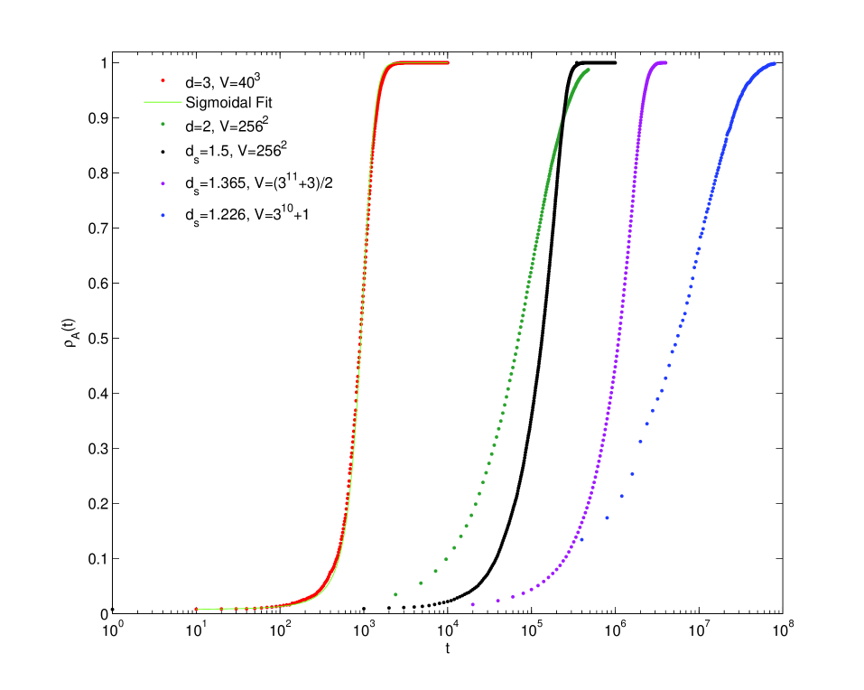
Figure 4: (Color online) Concentration of $A$ particles $\rho_{A}(t)$ vs time $t$ for a system made up of $N=128$ particles embedded on different structures, as shown by the legend. The best fit for the cubic lattice is also shown and it is given by a pure sigmoidal.

The mean-field extension just performed also allows to derive some insights into the temporal behavior displayed by $N_{A}(t)$. In fact, being $\tau_{n}$ the average time at which $N_{A}=n$, from Eq. 4 we can write

$$\tau_{n}=\displaystyle\sum_{N_{A}=1}^{n-1}\langle t_{N_{A}}\rangle=f(n).$$ (8)

Now, we estimate $N_{A}(t)$ as

$$N_{A}(t)=f^{-1}(t)$$

whose numerical solution provides an S-shaped curve to be compared (see Fig. 4) with the sigmoidal curve obtained from a standard mean-field approximation earlier1

$$N_{A}(t)=\frac{N}{(N-1)e^{-Npt}+1},$$ (9)

where $p$ is a quantity proportional to the concentration $\rho$ that in practice must be adjusted within the fitting procedure.

4 Simulations

In this section we show results obtained with numerical simulations performed on the Sierpinski gasket, on the T graph and on comb structures.

First of all we consider the dependence on $t$ displayed by $N_{A}(t)$. In Fig. 4 and 5 we show data obtained for the Sierpinski gasket. In particular, in the latter figure we also provide a comparison with results obtained for the T-graph, the comb lattice, the square lattice and the cubic lattice. Consistently with results found in earlier1 , for transient lattices $N_{A}(t)$ is well fitted by the sigmoidal function of Eq. 9, while for low-dimensional structures deviations are expected.

In fig.4 we show the time evolution $N_{A}(t)$ for substrates with the same total number of particles $N$ and with (approximately) the same volume $V$, but different spectral dimension $d$. In order of decreasing $d$, they are: the cubic lattice ($\tilde{d}=d=3$), the square lattice ($\tilde{d}=d=2$), the comb graph ($\tilde{d}=3/2$), the Sierpinski gasket fractal ($\tilde{d}=\frac{\log 9}{\log 5}\approx 1.365$) and the T-fractal ($\tilde{d}=\frac{\log 9}{\log 6}\approx 1.226$). We remind that the spectral dimension describes the long-range connectivity structure of the substrate and the long-time diffusive behavior of a random walker on the substrate. In particular, from Eq. 2, we expect that for substrates $\tilde{d}\leq 2$ the number of different sites visited by each walker will grow faster as $\tilde{d}$ increases, and so will the number of meetings between walkers. Hence, we expect the curves $N_{A}(t)$ to grow faster, and saturate earlier, with increasing $\tilde{d}$ ($N$ and $V$ being fixed). This is precisely what happens, as shown in Fig. 4 (except for the saturation time $\tau$ of the comb lattice, which will be discussed below). For $\tilde{d}\geq 2$ (e.g., $\tilde{d}=3$ in the figure), $N_{A}(t)$ is independent of $\tilde{d}$ and is fitted by a pure sigmoidal function.

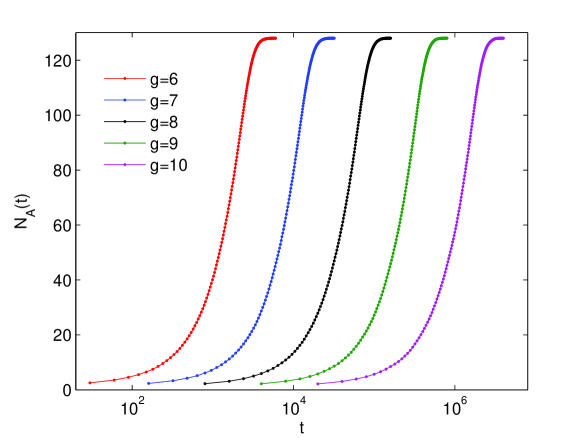
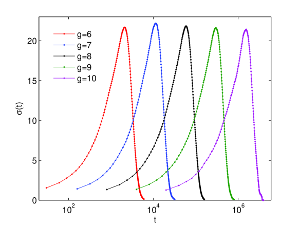
Figure 5: (Color online) Data depicted in the figures above refers to a system of $N=128$ particles diffusing on a Sierpinski gasket of five different generations. Each generations is depicted in different colors, as shown by the legend. Left: Number of $A$ particles $N_{A}(t)$ present in the system vs time $t$. Right: Fluctuations $\sigma(t)=\sqrt{\langle N_{A}^{2}\rangle-\langle N_{A}\rangle^{2}}$ as a function of time

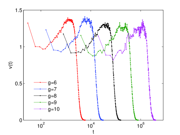
Figure 6: (Color online) Reaction velocity $v(t)$ for a system of $N=128$ particles diffusing on a Sierpinski gasket; five different generations (depicted in different colors) are shown. The reaction velocity is defined in Eq. 10

From $N_{A}(t)$ one can derive the rate of reaction

$$v(t)=\partial_{t}N_{A}(t).$$ (10)

As you can see from the numerical results in Fig. 6, in agreement with the theoretical one, $v(t)$ is an asymmetrical curve exhibiting a maximum at a time denoted by $t_{v}$. This time obviously corresponds to a flex in $N_{A}(t)$ which scales with the volume of the structure according to the following:

$$t_{v}\sim V^{2/\tilde{d}.}$$

This is the same dependence shown by $\tau$ (see below), and corresponds to a situation in which the population of the two species are about the same ($N_{A}=N_{B}=N/2$). Analogous results can be obtained for the T-fractal.

Furthermore, the profile shown in Fig. 6 also suggests that the efficiency of the autocatalytic reaction is not constant in time but, provided the number $N$ of particles is conserved, it exhibits a maximum when the number of $B$ particles is about $N/2$.

A similar result may be derived for the variance $\sigma_{A}(t)$ of the number of $A$ particles present on the substrate.

Interestingly, fluctuations display a maximum at a time $t_{\sigma}$ which, again, depends on the system size with the same law as $\tau$. Notice that $t_{\sigma}>t_{v}$ and $N_{A}(t_{v})=\frac{N}{2}.$

Finally, we consider the time $\tau$ representing the average time at which the autocatalytic reaction stops since all $B$ particles have been transformed into $A$ particles. In general this quantity depends on system parameters $V$ and $N=N_{A}+N_{B}$ and, as we will show, its functional form is significantly affected by the topology of the substrate.

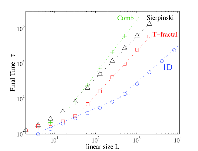
Figure 7: Scaling of $\tau$ with the linear size of the system for a 1-dimensional chain (blue circles), a Sierpinski gasket (black triangles), a T-fractal (red squares), and a comb lattice (green plus signs) on a double-logarithmic scale. The number of reactants is fixed at $N=1024$ for all systems. Dotted lines highlight the low-concentration regime ($L\gg 1$), corresponding to a power law for all systems. For the 1-dimensional chain, the linear high-concentration regime (low $L$) is also highlighted.

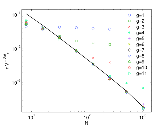
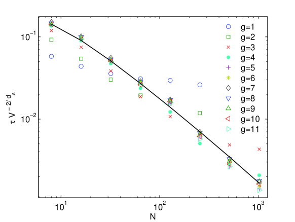
Figure 8: (Color online) Rescaled Final time $\tau V^{-2/\tilde{d}}$ vs number of particles $N$ for Sierpinski gasket (top) and T-fractal (bottom). Different symbols and colors distinguish different generation as explained by the legend. The line provides the best fit in agreement with equation 11.

The dependence of $\tau$ on the system size $L$ (or the volume $V=L^{d_{f}}$) clearly displays two different regimes, as shown in Fig. 7. In both cases, $\tau$ increases with $L$, but in the high-concentration regime the growth is less rapid; in particular (as shown for $d=1$ in the figure), it is proportional to $L$ for Euclidean lattices.

In the low-concentration regime, where we can assume that reactions only occur among two particles, the mean-field-like calculation explained in the previous section holds and we expect $\tau$ to vary with $N$ and $V$ according to Eq. 5 which can be rewritten as:

$$\tau V^{-2/\tilde{d}}=[\frac{1}{N}+N^{-2/\tilde{d}}(\log N-H_{\frac{2}{\tilde{d}}})].$$ (11)

Hence in Figure 8 we plotted $\tau V^{-2/\tilde{d}}$ vs $N$ and we fitted data according with the r.h.s . of the previous equation.

It can be seen that for small densities all the data collapse. Moreover, in that region, the fit coefficients introduced are in good agreement with theoretical predictions.

It should be underlined that the average final time depends non-trivially, on $N$ and $V$, viz. $\tau$ does not depend directly on the total concentration $\rho$, though the dependence on $N$ and $V$ can be factorized.

The agreement of formula 11 for the comb lattice is less good. In particular, it seems that the dependence of $\tau$ on $N$ and $V$ can still be factorized, but that the exponent for $V$ is rather $8/3$ than $2/\tilde{d}=4/3$. This may mean that the particular mean field approximation we have made does not hold anymore for strongly inhomogeneous structures such as combs; this point is still under investigation.

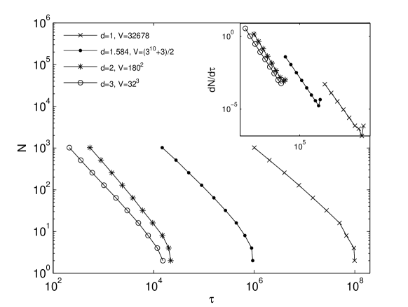
Figure 9: Loglog scale plot of the reactant amount $N$ vs Final time $\tau$; as shown in the legend, different substrate structures (with approximately the same volume) have been compared. In the inset the derivative $\frac{dN}{d\tau}$ is depicted again as a function of $\tau$. Lines are guides for the eyes.

As explained in Section 2, experimental measures of $\tau$ are useful in monitoring trace reactants. Indeed, our results show that $\tau=f_{\tilde{d}}(N)g_{\tilde{d}}(V)$ and therefore, once the substrate size is fixed, the initial amount of reactant can be expressed as $N=f_{\tilde{d}}^{-1}(\frac{\tau}{g_{\tilde{d}}(V)})$.

A proper estimate of the sensitivity of this method is provided by the derivative $\frac{dN}{d\tau}$: the smaller the derivative and the larger the sensitivity. In Fig. 9 we depicted numerical results for both $N$ and its derivative $\frac{dN}{d\tau}$ as a function of $\tau$; topologically different substrates are also compared, all sharing, approximately, the same volume. The numerical plots provided allows a qualitative analysis and comparison among the different structures considered; a more quantitative inspection can be outlined after a proper calibration procedure.

First of all, notice that the characteristic curves are well defined and they allows a univocal determination of $N$ from $\tau$. Moreover, the sensitivity of this analytic technique is better for small values of $N$ (with $N>2$) and, interestingly, for low-dimensional substrates. Indeed, once $V$ is fixed, when $d\leq 2$, the technique sensitivity is improved by lowering the substrate dimension. On the other hand, when $d>2$, the resulting curves are overlapped, hence no improvement is achieved. It should be underlined that the high sensitivity attained just for small concentrations of reactants makes this analytic technique very suitable for the determination of ultratrace amounts of reactants, which is of great experimental importance rose ; priest ; veer

5 Conclusions

We have presented a model that considers the autocatalytic reaction $A+B\rightarrow 2\,A$ on non-Euclidean, low-dimensional ($\tilde{d}<2$), finite-size substrates, characterized by a volume $V$ and a total number of reacting particles $N$.

We showed by analytical calculations that the Final Time $\tau$ (the total time span of the reaction) displays two different regimes, for high and low concentrations, with a different dependence on $V$ and $N$. In particular, the functional law for low concentrations can be recovered by means of a mean-field approximation. In fact, with respect to the standard one, our mean-field approach is able to take into account the topological effect arising from a low-dimensional substrate.

Numerical simulations corroborated these results for fractals, while simulations on strongly inhomogeneous lattices (combs) hint at a quantitatively different behavior.

Theoretical results concerning the average Final Time find important applications in analytical fields, where measures of $\tau$ are exploited for detecting trace reactants. Our results suggest that the sensitivity of such technique is affected not only by the reactant concentration, but also by the topology of the structure underlying diffusion. More precisely, a small concentration of reactants implies a better sensitivity, hence allowing the determination of ultra-trace reactants. Moreover, at the same concentration, and for low-dimensional ($d<2$) substrates, by reducing the dimension $d$ the sensitivity can be further improved.

References

- (1) Bartumeus F, Catalan J, Fulco UL, Lyra ML and Viswanathan GM (2002) Phys Rev Lett 88:097901
- (2) Hess B and Mikhailov A (1994) Science 264:223.
- (3) Acedo L, Yuste SB (2001) Phys Rev E 63:011105
- (4) Toussaint D, Wilczek F (1983) J Chem Phys 78:2642
- (5) Gennes PG, J Chem Phys 76:3316
- (6) Blumen A, Klafter J, Zumofen G (1983) Phys Rev B 28:6112
- (7) Zumofen G, Blumen A, Klafter J, J Chem Phys 82:3198 (1985)
- (8) Lindenberg K, Sheu W-S, Kopelman R (1991) Phys Rev A 43:7070
- (9) Zumofen G, Klafter J, Blumen A (1991) Phys Rev A 44:8390
- (10) Lemarchand A, Lemarchand H, Sulpice S, Mareshal M (1992) Physica A 188:277
- (11) Mai J, Sokolov IM, Blumen A (2000) Phys Rev E 62:141
- (12) Mai J, Sokolov IM, Blumen A (1998) Europhys Lett 4:7
- (13) Velikanov MV, Kapral R (1998) J Chem Phys 110:109
- (14) Warren CP, Mikus G, Somfai E, Sander LM (2001) Phys Rev E 63:056103
- (15) Chaivorapoj W, Birol İ, Teymour F (2002) Ind Eng Chem Res 41:3630
- (16) Fisher RA (1937) Ann. Eugenics 7:335
- (17) Kolmogorov A, Petrovsky I, Piskunov P (1937) Bull Univ Moscow Ser Int Sec A 1:1
- (18) Agliari E, Burioni R, Cassi D, Neri FM (2006) Phys Rev E 73:046138
- (19) Agliari E, Burioni R, Cassi D, Neri FM (2007) Phys Rev E 75:021119
- (20) Endo M, Abe S, Deguchi Y, Yotsuyanagi T (1998) Talanta 47:349
- (21) Ichimura K, Arimitsu K, Tahara M (2004) J Materials Chemistry 14:1164
- (22) Merkin JH, Poole AJ, Scott SK, Masere J, Showalter K (1998) J Chem Soc Faraday Trans 94:53
- (23) Singh V, Singh J, Kaur KP, Kad GL (1996) J Chem Research, 58
- (24) Ishihara M, Endo M, Igarashi S, Yotsuyanagi T (1995) Chemistry Letters, 349
- (25) Kato J, Ohno O, Igarashi S (2005) Analytical Sciences, 21:705
- (26) Havlin S, ben Avraham D (2000) Diffusion and Reactions in Fractals and Disordered Systems, Cambridge University Press
- (27) C. van den Broek (1989) Phys Rev A 40:7334
- (28) Oshanin G, Benichou O, Coppe M, Moreau M (2002) Phys Rev E 66:060101(R)
- (29) Rose A, Zhu Z, Madigan CF, Swager TM, Bulovic V (2005) Nature, 434:876
- (30) Priest ND J Environ Monit 2002, 6:375
- (31) McKeachie JR, van der Veer WR, Short LC, Garnica RM, Appel MF and Benter T (2001) Analyst, 126:1221