Protected Rabi oscillation induced by natural interactions among physical qubits

Abstract

For a system composed of nine qubits, we show that natural interactions among the qubits induce the time evolution that can be regarded, at discrete times, as the Rabi oscillation of a logical qubit. Neither fine tuning of the parameters nor switching of the interactions is necessary. Although straightforward application of quantum error correction fails, we propose a protocol by which the logical Rabi oscillation is protected against all single-qubit errors. The present method thus opens a simple and realistic way of protecting the unitary time evolution against noise.

I Introduction

Decoherence of quantum states has been attracting much attention for long years SM02 . Many methods have been proposed for defeating the decoherence. As compared with other methods ZR97 ; KBLW01 ; VKL99 ; Facchi05 , quantum error correction (QEC) Sh95 ; St96 ; NC00 ; Go97 ; Pre98 has a great advantage of protecting against arbitrary errors if they only affect a single qubit (two-level system) in each logical qubit NC00 . Although QEC has been developed in the context of quantum computation, it is interesting and useful to apply QEC to protection of the unitary time evolution (Hamiltonian evolution) against noise.

When trying to realize this, however, one encounters many physical problems, which are usually disregarded in discussions on the computational complexity NC00 . For example, some physical process may be much more difficult to realize than another, even if the number of the necessary steps for them differs ‘only by polynomial steps’ NC00 . Furthermore, fabrication of a controlled-NOT gate, which is one of the elementary quantum gates, is very difficult because it requires fine tuning of the coupling constants of the interactions and high-precision switching of them, even if one employs the excellent ideas of Refs. DiV00 ; ML05 . Assembling a quantum circuit from the elementary gates is even more difficult, particularly when the circuit is large and complicated. Unfortunately, the circuit indeed becomes large and complicated when one tries to apply QEC to the Hamiltonian evolution, even for the simplest case such as the Rabi oscillation Pre98 . The largest and most complicated part of the circuit is the one that induces the encoded Hamiltonian evolution (such as the Rabi oscillation of a logical qubit) in a fault-tolerant manner NC00 ; Go97 . Although a non-fault-tolerant circuit can be much simpler, such a circuit is too fragile to errors. It is therefore important to explore new methods, which are physically more feasible and natural, for inducing the encoded Hamiltonian evolution and thereby making QEC applicable.

In this paper, we propose such a new method, choosing the Rabi oscillation as the Hamiltonian evolution to be protected. The method utilizes effective interactions that arise naturally among physical qubits. We show that the values of the parameters in the interactions are to a great extent arbitrary. Furthermore, switching of the interactions is unnecessary. Therefore, a system of a logical qubit with such interactions can be prepared easily by placing several two-level systems close to each other. Once such a system is prepared, it is driven spontaneously and flawlessly by the Schrödinger equation. This is much easier than to drive the system by a fault-tolerant quantum circuit. On the other hand, we argue physically that it is highly probable that unwanted interactions should also exist in such a system. While some of them are shown to be irrelevant, the others invalidate straightforward application of QEC. As a resolution we present a protocol, which we call the error-correction sequence. One can realize the protected Rabi oscillation by using the natural interactions (to induce the logical Rabi oscillation) and a quantum circuit for the error-correction sequence. This is much easier than realizing it wholly with a quantum circuit, because a fault-tolerant quantum circuit for inducing the logical Rabi oscillation, which is the largest and most complicated part of the full circuit, is unnecessary.

II Natural Hamiltonian for logical Rabi oscillation

We employ a two-level system as a basic element, which we call a qubit or physical qubit. We represent operators acting on a qubit in terms of the Pauli operators $X,Y,Z$ (i.e., $\sigma_{1},\sigma_{2},\sigma_{3}$), which are not necessarily those for a physical spin. To apply QEC to the Rabi oscillation,

$$e^{i\omega Xt}|0\rangle=\cos(\omega t)|0\rangle+i\sin(\omega t)|1\rangle,$$ (1)

we replace a single qubit with a logical qubit which is composed of several qubits. The basis states $|0\rangle,|1\rangle$ ($+1$ and $-1$ eigenstate of $Z$, respectively) of a qubit correspond to $|0_{L}\rangle,|1_{L}\rangle$ of a logical qubit. The subspace (of the logical qubit) that is spanned by the latter is called the code space. For the reasons that will be described in Sec.VII, we here take the Shor code Sh95 , in which a logical qubit is composed of nine qubits and

$$|0_{L}\rangle = {\bigl{(}|000\rangle+|111\rangle\bigr{)}\bigl{(}|000\rangle+|111\rangle\bigr{)}\bigl{(}|000\rangle+|111\rangle\bigr{)}\over 2^{3/2}},$$ (2)

$$|1_{L}\rangle = {\bigl{(}|000\rangle-|111\rangle\bigr{)}\bigl{(}|000\rangle-|111\rangle\bigr{)}\bigl{(}|000\rangle-|111\rangle\bigr{)}\over 2^{3/2}}.$$ (3)

We have to induce the logical Rabi oscillation;

$$e^{i\omega X_{L}t}|0_{L}\rangle=\cos(\omega t)|0_{L}\rangle+i\sin(\omega t)|1_{L}\rangle,$$ (4)

where $X_{L}$ is a logical Pauli operator; $X_{L}|0_{L}\rangle=|1_{L}\rangle$ and $X_{L}|1_{L}\rangle=|0_{L}\rangle$. Obviously, it can be induced if the Hamiltonian is $-\omega X_{L}$. [Here and after, we take $\hbar=1$.] This is an interaction among three or more qubits, for any code that can correct all single-qubit errors (Appendix A). For the Shor code, $X_{L}$ can be represented in various ways, e.g., as $X_{L}=Z_{3}Z_{6}Z_{9}$ or $\Pi_{i=1}^{9}Z_{i}$, where $Z_{i}$ acts on qubit $i$. In the following, we take

$$X_{L}=Z_{1}Z_{4}Z_{7}.$$ (5)

Suppose that nine qubits (such as atoms, quantum dots, and so on) composing a logical qubit are placed close to each other as shown in Fig. 1. Then, as will be discussed in Sec. VI, a three-qubit interaction proportional to $X_{L}$ ($=Z_{1}Z_{4}Z_{7}$) would be generated as an effective interaction. [Similar three-qubit interactions were also discussed in Refs. 3body1 ; 3body2 .] Unfortunately, however, if this interaction is strong enough unwanted two-qubit interactions proportional to $Z_{1}Z_{4},Z_{4}Z_{7},Z_{7}Z_{1}$ should also be strong, because otherwise the following unphysical conclusion would be drawn; if one of qubits $1,4,7$ is removed the other two qubits would have no interactions. Furthermore, interactions between other pairs of qubits, such as $Z_{1}Z_{2},Z_{2}Z_{3},\cdots$, would also exist in general. Therefore, a natural and simple Hamiltonian for the system of Fig. 1 is

$$H=H_{D}+H_{S},$$ (6)

where

$$H_{D}=-\omega Z_{1}Z_{4}Z_{7}-J(k_{1}Z_{1}Z_{4}+k_{4}Z_{4}Z_{7}+k_{7}Z_{7}Z_{1}),$$ (7)

$$H_{S}=\sum_{s=2,3,5,6,8,9}g_{s}Z_{s-1}Z_{s}.$$ (8)

Here, $\omega$, $J$, $k_{r}$’s, $g_{s}$’s are real parameters. Since the signs of these parameters are irrelevant to the following discussions, we assume without loss of generality that they are positive. Furthermore, since three-qubit interactions are generally weaker than two-qubit interactions (see Sec. VI), we assume naturally that

$$0<\omega\ll J.$$ (9)

Although single-qubit terms may also exist, we can forget them because, as discussed in Appendix B, they are irrelevant to the following discussions.

Figure 1: An example of the configuration of qubits that have the proposed Hamiltonian. The distances between the qubits are to a large extent arbitrary. We label the qubits inside and outside the central triangle by $r$ ($=1,4,7$) and $s$ ($=2,3,5,6,8,9$), respectively.

Note that the operators $Z_{s-1}Z_{s}$ in $H_{S}$ do not change $|0_{L}\rangle$ or $|1_{L}\rangle$, i.e., they are elements of the stabilizer Go97 of the Shor code. Using this fact, we will show later by explicit calculations that the values of $g_{s}$’s are irrelevant. On the other hand, the two-qubit interactions in $H_{D}$ are not elements of the stabilizer, and hence drive the state out of the code space. Nevertheless, we will show in Sec. V that the values of $J$ and $k_{r}$’s are fairly arbitrary as long as $\omega\ll J$. The value of $\omega$ is also unimportant because changing $\omega$ is just equivalent to changing the time scale. Therefore, the values (including signs) of all the parameters in $H$ (hence the distances between the qubits) are to a great extent arbitrary. This makes our scheme robust to fabrication errors. Once the system is thus fabricated, the law of the Nature drives it flawlessly if noise is absent.

III Difficulties and resolutions

We now discuss effects of noise. There are two difficulties in applying QEC straightforwardly to the system driven by $H$. We now explain them and resolutions. For simplicity, we explain the case where $k_{1}=k_{4}=k_{7}=1$. More general cases will be discussed in Sec. V.

We study the first difficulty by investigating the time evolution in the absence of noise, i.e., we calculate $|\psi(t)\rangle\equiv e^{-iHt}|\psi_{L}^{0}\rangle$, where $|\psi_{L}^{0}\rangle$ is a vector in the code space. We note that all terms in $H$ commute with each other, and that $H_{S}$ does not change $|\psi_{L}^{0}\rangle$ because all terms in $H_{S}$ are elements of the stabilizer. Using these facts and the relations $Z_{1}Z_{4}=Z_{7}X_{L},Z_{4}Z_{7}=Z_{1}X_{L},Z_{7}Z_{1}=Z_{4}X_{L}$, we find

$$|\psi(t)\rangle= \left\{\cos^{3}(Jt)-i\sin^{3}(Jt)\right\}e^{i\omega tX_{L}}|\psi_{L}^{0}\rangle$$

$$+\frac{i}{2}\sum_{r=1,4,7}e^{iJt}\sin(2Jt)Z_{r}X_{L}e^{i\omega tX_{L}}|\psi_{L}^{0}\rangle.$$ (10)

When $\sin(2Jt)\neq 0$, this state is out of the code space because of the last term. Therefore, we cannot perform QEC for phase errors at an arbitrary time, because the syndrome measurement NC00 to identify the errors misidentifies the last term as a wrong term generated by a phase-flip noise; if QEC for phase errors were performed with some intervals $\mu$ the time evolution would be affected as shown in Fig. 2, even when noise is absent.

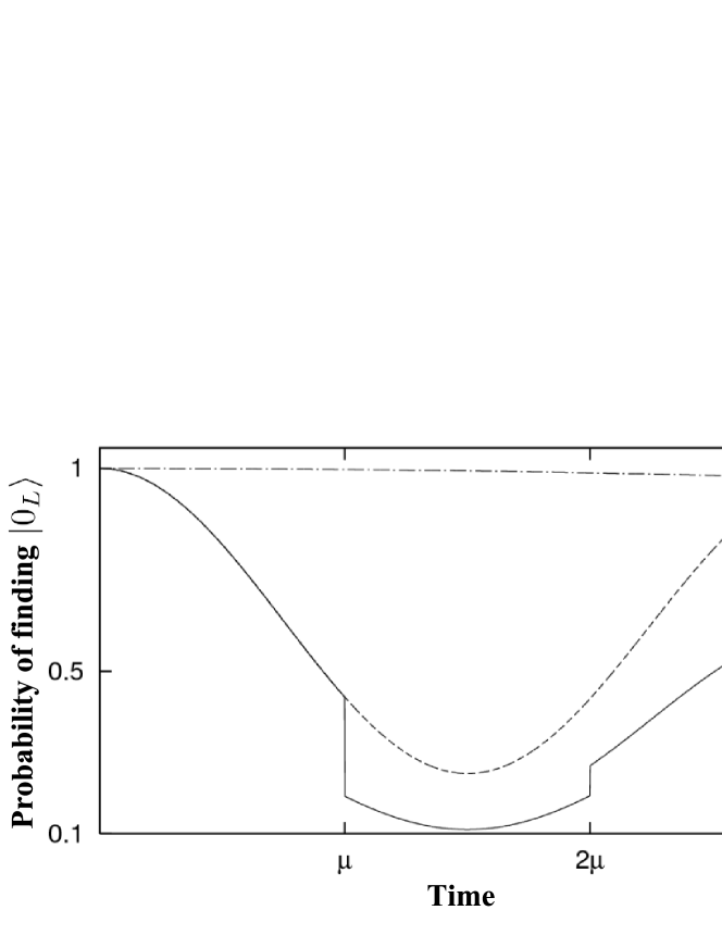
Figure 2: Probability of finding $|0_{L}\rangle$ plotted against time, for the logical Rabi oscillation (chain line), the Hamiltonian evolution by $H$ (dashed line), that affected by QEC for phase errors (solid line), which is performed repeatedly with some intervals $\mu$.

However, if we focus on the discrete times

$$t_{m}\equiv m\tau\quad(m=0,1,2,\cdots),$$ (11)

then $|\psi(t_{m})\rangle$ is in the code space, where

$$\tau\equiv\pi/2J.$$ (12)

Therefore, we can perform QEC at $t=t_{m}$, for both phase and bit-flip errors. Furthermore, since

$$|\psi(t_{m})\rangle=e^{i\omega t_{m}X_{L}}|\psi_{L}^{0}\rangle=\left[\cos(\omega t_{m})+i\sin(\omega t_{m})X_{L}\right]|\psi_{L}^{0}\rangle$$ (13)

apart from an irrelevant phase factor, the logical Rabi oscillation is realized at these discrete times, which we call the discrete logical Rabi oscillation. Since $\omega/J\ll 1$, the intervals $\tau$ of the discrete times are much shorter than the period $2\pi/\omega$ of the Rabi oscillation. Hence, the discrete logical Rabi oscillation $\{|\psi(t_{m})\rangle\}_{m=0,1,2\cdots}$ is quasi continuous as shown by the dots in Fig. 3.

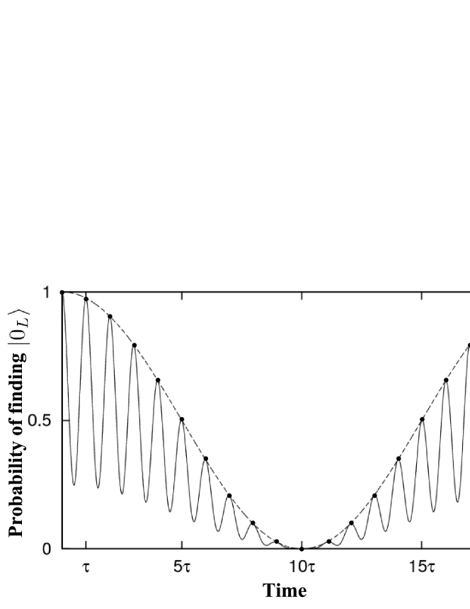
Figure 3: Probability of finding $|0_{L}\rangle$ plotted against time, for the logical Rabi oscillation (chain line) and the Hamiltonian evolution by $H$ (solid line). For clarity, we take $\omega/J$ ($\ll 1$) not so small; $\omega/J=0.1$. The dots represent the discrete logical Rabi oscillation.

To discuss the second difficulty, let us study the time evolution in the presence of noise. Suppose, e.g., that the system has evolved freely from noise for $t<t^{\prime}$, where $t_{m-1}<t^{\prime}<t_{m}$, until a bit-flip noise $X_{1}$ acts on qubit $1$ at $t^{\prime}$. Then the state at $t_{m}$ is evaluated as

$$e^{-iH(t_{m}-t^{\prime})}X_{1}e^{-iHt^{\prime}}|\psi_{L}^{0}\rangle$$

$$\quad=e^{-i\left[g_{2}(2t^{\prime}-t_{m})+\sum_{s\neq 2}g_{s}t_{m}\right]}X_{1}e^{iJ(2t^{\prime}-t_{m})(Z_{1}Z_{4}+Z_{7}Z_{1})}$$

$$\quad\quad\times(iZ_{4}Z_{7})^{m}e^{i\omega(2t^{\prime}-t_{m})X_{L}}|\psi_{L}^{0}\rangle.$$ (14)

The terms proportional to $g_{s}$’s are irrelevant because they contribute only to an overall phase factor. Therefore, $g_{s}$’s may take arbitrary values. The problem is that the above state is different from the correctable state $X_{1}|\psi(t_{m})\rangle$, not only in the term generated by $Z_{1}Z_{4}+Z_{7}Z_{1}$ and $(iZ_{4}Z_{7})^{m}$ but also in the wrong phase of the oscillation $\omega(2t^{\prime}-t_{m})$. That is, extra errors occur because the bit-flip error in qubit $1$ (or $4$ or $7$) is ‘propagated’ by $H$ to other qubits . As a result, QEC at $t_{m}$ cannot recover the correct state.

To overcome this difficulty, we note that the syndrome measurement for bit-flip errors (unlike that for phase errors) does not misidentify the state of Eq. (10) as a wrong state. Hence, one can successfully perform QEC for bit-flip errors frequently (i.e., with intervals $\nu$ which are much shorter than $\tau$) in the interval between $t_{m-1}$ and $t_{m}$ for all $m$. As will be confirmed in the next section, this reduces the probability of errors small enough.

Our prescription is summarized as follows: Perform QEC for both phase and bit-flip errors at all $t_{m}$’s (i.e., with intervals $\tau$), and perform QEC for bit-flip errors repeatedly with intervals $\nu$ ($\ll\tau$). The latter intervals $\nu$ are not required to be regular. We call this protocol the error-correction sequence.

IV Effects of the error-correction sequence

To see how well the error-correction sequence protects the discrete logical Rabi oscillation against noise, let us calculate the time evolution for $t_{0}<t\leq t_{1}$, i.e., for $0<t\leq\tau$, quantitatively.

We divide the interval $(0,t]$ into $N$ subintervals; $(0,\Delta t],(\Delta t,2\Delta t],(2\Delta t,3\Delta t],\cdots$, where $\Delta t\equiv t/N$. We model noise by the product of depolarizing channels NC00 $\Pi_{i=1}^{9}{\cal E}_{\Delta t}^{(i)}$, where ${\cal E}_{\Delta t}^{(i)}$ acts on qubit $i$ at the end of every subinterval as

$${\cal E}_{\Delta t}^{(i)}[\rho]\equiv(1-\epsilon\Delta t)\rho+{\epsilon\Delta t\over 3}\sum_{\alpha=1}^{3}\sigma_{\alpha}^{(i)}\rho\sigma_{\alpha}^{(i)}.$$ (15)

Here, $\rho$ denotes an input state, and $\epsilon$ is a small positive parameter representing the strength of the interaction with the environment. The initial state at $t=0$ is denoted by $\rho_{L}^{0}$, which is assumed to be in the code space. We study its time evolution up to the first orders in $\epsilon\tau$ and $\omega\tau$, assuming that

$$\epsilon\tau\ll 1\mbox{ and }\omega\tau\ll 1,$$ (16)

where the latter comes from condition (9).

If noise and QEC were absent, $\rho_{L}^{0}$ would evolve into

$$\rho_{H}(t)\equiv e^{-iHt}\rho_{L}^{0}e^{iHt}=e^{-iH_{D}t}\rho_{L}^{0}e^{iH_{D}t}.$$ (17)

When noise is present but QEC is not performed, on the other hand, $\Pi_{i=1}^{9}{\cal E}_{\Delta t}^{(i)}$ acts at the end of every subinterval. When $N=2$, for example, $\rho_{L}^{0}$ evolves into

$$\prod_{i=1}^{9}{\cal E}_{\Delta t}^{(i)}\left[e^{-iH\Delta t}\prod_{i=1}^{9}{\cal E}_{\Delta t}^{(i)}\left[\rho_{H}(\Delta t)\right]e^{iH\Delta t}\right]$$ (18)

$$=(1-9\epsilon t)\rho_{H}(t)+\frac{\epsilon}{3}\sum_{j=1}^{2}\Delta te^{-iH(t-j\Delta t)}\sum_{i=1}^{9}\sum_{\alpha=1}^{3}\sigma_{\alpha}^{(i)}\rho_{H}(j\Delta t)\sigma_{\alpha}^{(i)}e^{iH(t-j\Delta t)}.$$ (19)

By taking $N\rightarrow\infty$, we obtain the state at $t$ without QEC as

$$\rho(t,\rho_{L}^{0})\simeq (1-9\epsilon t)\rho_{H}(t)$$

$$+\frac{\epsilon}{3}\int_{0}^{t}dt^{\prime}\,e^{-iH(t-t^{\prime})}\sum_{i=1}^{9}\sum_{\alpha=1}^{3}\sigma_{\alpha}^{(i)}\rho_{H}(t^{\prime})\sigma_{\alpha}^{(i)}e^{iH(t-t^{\prime})}.$$ (20)

We calculate how this state is corrected by the error-correction sequence, in which bit-flip errors are corrected with intervals $\nu$ and both bit-flip and phase errors are corrected at $t=\tau$. Although the intervals $\nu$ are not required to be regular, and

$$n\equiv\tau/\nu$$ (21)

is not required to take an integral value, we here assume for simplicity that $\nu$ is regular and $n$ is an integer. We label qubits in and outside the central triangle of Fig. 1 by $r,r^{\prime}$ ($=1,4,7$) and $s$ ($=2,3,5,6,8,9$), respectively.

At $t=\nu$, QEC for bit-flip errors is performed. The pre-measurement state of the syndrome measurement is $\rho(\nu,\rho_{L}^{0})$. The post-measurement state $\rho^{\prime}(\nu)$ depends on the outcome of the syndrome measurement. For example, when the bit-flip error in qubit $s$ is detected (which happens with probability $2\epsilon\nu/3$),

$$\rho^{\prime}(\nu)=\frac{1}{2}X_{s}\rho_{H}(\nu)X_{s}+\frac{1}{2}Y_{s}\rho_{H}(\nu)Y_{s}.$$ (22)

By the recovery operation, $\rho^{\prime}(\nu)$ is changed into

$$\rho^{\prime\prime}(\nu)\equiv X_{s}\rho^{\prime}(\nu)X_{s}=\frac{1}{2}\rho_{H}(\nu)+\frac{1}{2}Z_{s}\rho_{H}(\nu)Z_{s},$$ (23)

which is a mixture of the correct state $\rho_{H}(\nu)$ and $Z_{s}\rho_{H}(\nu)Z_{s}$, the state with a phase error in qubit $s$. At this stage, QEC for phase error is not performed because $\rho_{H}(\nu)$ is out of the code space.

At $t=2\nu$, QEC for bit-flip errors is performed again. The pre-measurement state is $\rho(\nu,\rho^{\prime\prime}(\nu))$, where $\rho^{\prime\prime}(\nu)$ corresponds to one of possible outcomes of the previous syndrome measurement at $t=\nu$. We can calculate $\rho^{\prime}(2\nu)$ and $\rho^{\prime\prime}(2\nu)$ in the same way as we have calculated $\rho^{\prime}(\nu)$ and $\rho^{\prime\prime}(\nu)$. By repeating the arguments $n$ times, we obtain the probabilities of bit-flip errors during $0<t<\tau$ and the corresponding states $\rho^{\prime\prime}(\tau)$ that are obtained at $t=n\nu=\tau$ by correcting the bit-flip errors. To the first orders in $\epsilon\tau$ and $\omega\tau$, they are given by

$$\begin{array}[]{ccc}\hline\cr\mbox{error}&\mbox{probability}&\mbox{corrected state }\rho^{\prime\prime}(\tau)\\ \hline\cr\mbox{none}&1-6\epsilon\tau&(1-3\epsilon\tau)\rho_{H}(\tau)+\frac{\epsilon\tau}{3}\sum_{i}Z_{i}\rho_{H}(\tau)Z_{i},\\ X_{s}&2\epsilon\tau/3&\frac{1}{2}\rho_{H}(\tau)+\frac{1}{2}Z_{s}\rho_{H}(\tau)Z_{s},\\ X_{r}&2\epsilon\tau/3&\frac{1}{2}\rho_{e}^{(r)}(\tau)+\frac{1}{2}Z_{r}\rho_{e}^{(r)}(\tau)Z_{r},\vspace{1mm}\\ \hline\cr\end{array}$$ (24)

where

$$\rho_{e}^{(r)}(\tau)\equiv\int_{0}^{\nu}e^{2iJZ_{r}X_{L}t^{\prime}}\rho_{H}(\tau-2t^{\prime})e^{-2iJZ_{r}X_{L}t^{\prime}}\frac{dt^{\prime}}{\nu}.$$ (25)

Finally at $t=\tau$, phase errors in $\rho^{\prime\prime}(\tau)$ are detected and corrected. We denote the state after this QEC by $\rho^{\prime\prime\prime}(\tau)$. Since $\rho^{\prime\prime}(\tau)$ depends on which qubit has suffered from a bit-flip error for $0<t<\tau$, so does $\rho^{\prime\prime\prime}(\tau)$. If a bit-flip error has occurred in no qubit or in qubit $s$, $\rho^{\prime\prime\prime}(\tau)$ agrees with the correct state $\rho_{H}(\tau)$. If, on the other hand, a bit-flip error has occurred in qubit $r$ (with probability $2\epsilon\tau/3$, see above), the conditional probability of each outcome of the syndrome measurement for phase errors and the corresponding $\rho^{\prime\prime\prime}(\tau)$ are given by

$$\begin{array}[]{ccc}\hline\cr\mbox{error}&\mbox{probability}&\mbox{corrected state }\rho^{\prime\prime\prime}(\tau)\\ \hline\cr\mbox{none or }Z_{r}&\frac{3}{8}+\frac{1}{8}{\rm sinc}\frac{\displaystyle 4\pi}{\displaystyle n}&{\displaystyle\frac{a_{n}^{+}\rho_{H}(\tau)+a_{n}^{-}X_{L}\rho_{H}(\tau)X_{L}}{a_{n}^{+}+a_{n}^{-}}},\\ Z_{r^{\prime}}\ (r^{\prime}\neq r)&\frac{1}{8}-\frac{1}{8}{\rm sinc}\frac{\displaystyle 4\pi}{\displaystyle n}&\frac{1}{2}\left[\rho_{H}(\tau)+X_{L}\rho_{H}(\tau)X_{L}\right].\vspace{1mm}\\ \hline\cr\end{array}$$ (26)

Here, ${\rm sinc}\,x\equiv(\sin x)/x$, $a_{n}^{\pm}\equiv\frac{3}{16}+\frac{1}{16}{\rm sinc}{4\pi\over n}\pm\frac{1}{4}{\rm sinc}{2\pi\over n}$, and terms of $O(\epsilon\tau)$ and $O(\omega\tau)$ have been dropped because the probability that a bit-flip error has occurred is already of $O(\epsilon\tau)$. By averaging $\rho^{\prime\prime\prime}(\tau)$ over all possible branches, we obtain the average state $\rho_{c}(\tau)$ under the error-correction sequence as

$$\rho_{c}(\tau)=\rho_{H}(\tau)-\epsilon\tau\left[1-{\rm sinc}\frac{2\pi}{n}\right]\left[\rho_{H}(\tau)-X_{L}\rho_{H}(\tau)X_{L}\right].$$ (27)

Therefore, $\rho_{c}(\tau)$ approaches the correct state $\rho_{H}(\tau)$ with increasing $n$. This can be seen more clearly from their trace distance NC00 , which is calculated for $n\gg 1$ as

$${1\over 2}{\rm tr}\left|\rho_{c}(\tau)-\rho_{H}(\tau)\right|\simeq 2\pi^{2}\epsilon\tau L_{yz}(\tau)/3n^{2}.$$ (28)

Here, $L_{yz}(\tau)$ denotes the length of the projection onto the $y$-$z$ plane of the Bloch vector of $\rho_{H}(\tau)$ in the code space. Hence, by taking

$$n\gtrsim(1/\sqrt{\epsilon\tau})\min\{1,\epsilon/\omega\},$$ (29)

we can reduce the distance to about $6L_{yz}(\tau)\max\{(\epsilon\tau)^{2},(\omega\tau)^{2}\}$. Since $L_{yz}(\tau)=O(1)$, this is of the same order as the largest term that has been dropped in the above calculations. That is, we have successfully recovered the correct state at $t=\tau$ ($=t_{1}$), i.e., $\rho_{c}(t_{1})=\rho_{H}(t_{1})+O\left(\max\{(\epsilon\tau)^{2},(\omega\tau)^{2}\}\right)$.

In a similar manner, we can evaluate $\rho_{c}(t_{m})$ by taking $\rho_{c}(t_{m-1})$ as the initial state, and find that

$$\rho_{c}(t_{m})=\rho_{H}(t_{m})+O\left(\max\{(\epsilon\tau)^{2},(\omega\tau)^{2}\}\right)$$ (30)

for all $m$. Therefore, the discrete logical Rabi oscillation is protected, with only $O\left(\max\{(\epsilon\tau)^{2},(\omega\tau)^{2}\}\right)$ probability of failure, if we take $n$ as Eq. (29). For example, we should take $n\gtrsim 10^{2}$ when $\epsilon\tau=\omega\tau=10^{-4}$.

Figure 4 demonstrates how the error-correction sequence corrects errors, i.e., how the solid line approaches the dashed line.

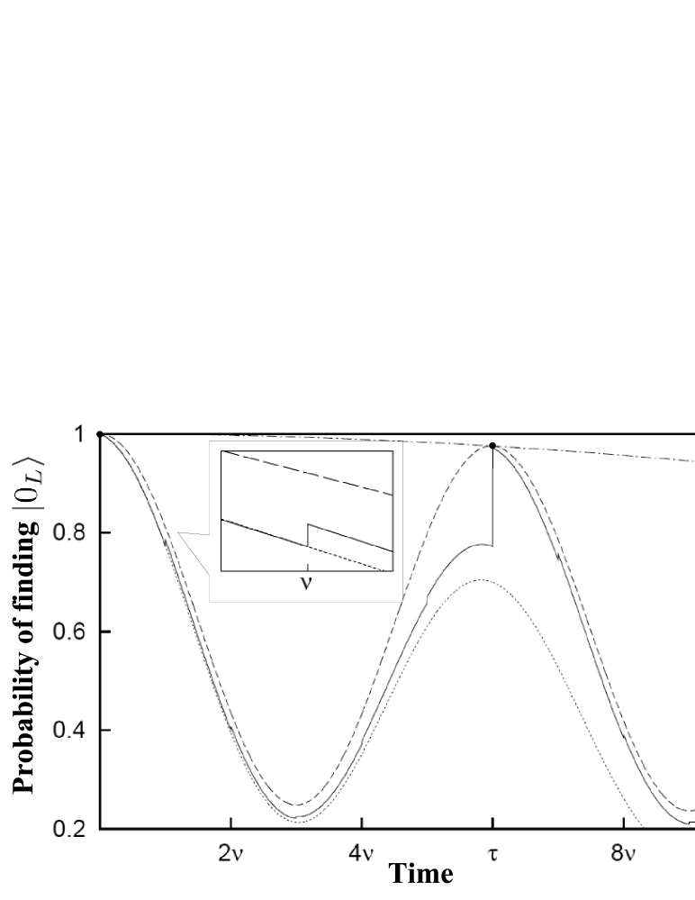
Figure 4: Probability of finding $|0_{L}\rangle$ plotted against time when $\rho_{L}^{0}=|0_{L}\rangle\langle 0_{L}|$, for the logical Rabi oscillation (chain line), the Hamiltonian evolution by $H$ (dashed line), that affected by noise (dotted line), and that corrected by the error-correction sequence (solid line). The dots represent the discrete logical Rabi oscillation. Here, $\omega/J=0.1$, $\epsilon\tau=\pi/100$, $\tau/\nu=6$. Inset: magnification around $t=\nu$.

V Arbitrariness of the parameters in $H_{D}$

It is clear from the results of Secs. III and IV that the value of $J$ is arbitrary as long as $\omega\ll J$. On the other hand, we have assumed in those sections that $k_{1}=k_{4}=k_{7}=1$. In this section, we show that the error-correction sequence is successful also when $k_{r}$’s take other values.

Recall that the error-correction sequence consists of two parts; QEC for both phase and bit-flip errors at all $t_{m}$’s, and QEC only for bit-flip errors with intervals $\nu$. The latter part is successful even when $k_{r}$’s are arbitrary real numbers, because in general a Hamiltonian which does not contain $X_{i}$’s and $Y_{i}$’s, such as the proposed $H$, cannot flip the bit of any physical qubit. Hence, the syndrome measurement for bit-flip errors does not misidentify the state evolved by such a Hamiltonian as a wrong state.

Regarding the former part, we start with showing that $k_{r}$’s can be arbitrary integers. Note that QEC at $t_{m}$’s works well provided that the state of the qubits at $t_{m}$ would be in the code space if noise were absent. As discussed in Sec. III, this condition is satisfied when $k_{1}=k_{4}=k_{7}=1$, because $|\psi(t_{m})\rangle=e^{i\omega t_{m}X_{L}}|\psi_{L}^{0}\rangle$, which is certainly in the code space. When $k_{r}$’s are odd integers, we obtain the same result;

$$|\psi(t_{m})\rangle = e^{-iH_{D}t_{m}}|\psi_{L}^{0}\rangle$$ (31)

$$= e^{i\omega t_{m}X_{L}}e^{i\frac{m\pi}{2}(k_{1}Z_{1}Z_{4}+k_{4}Z_{4}Z_{7}+k_{7}Z_{7}Z_{1})}|\psi_{L}^{0}\rangle$$

$$= e^{i\omega t_{m}X_{L}}\prod_{r=1,4,7}\left[\cos\frac{mk_{r}\pi}{2}+i\sin\frac{mk_{r}\pi}{2}Z_{r}Z_{r+3}\right]|\psi_{L}^{0}\rangle$$

$$= e^{i\omega t_{m}X_{L}}|\psi_{L}^{0}\rangle,$$

apart from irrelevant phase factors. Here, $Z_{10}\equiv Z_{1}$, and we have used $(Z_{1}Z_{4})(Z_{4}Z_{7})(Z_{7}Z_{1})=1$. When $k_{r}$’s are general integers (not necessarily odd), on the other hand, we have to add a certain procedure to the error correction sequence. We explain this for the case where $k_{1}=1$ and either one of $k_{4},k_{7}$ is even. In this case, we find that

$$|\psi(t_{m})\rangle=\begin{cases}e^{i\omega t_{m}X_{L}}|\psi_{L}^{0}\rangle&\mbox{for even $m$},\\ Z_{r}Z_{r^{\prime}}e^{i\omega t_{m}X_{L}}|\psi_{L}^{0}\rangle&\mbox{for odd $m$}.\end{cases}$$ (32)

Here, $r$ and $r^{\prime}$ $(\neq r)$ each is $1,4$ or $7$ depending on $k_{4},k_{7}$. For example, when $k_{4}$ is even and $k_{7}$ is odd, $|\psi(t_{m})\rangle=Z_{7}Z_{1}e^{i\omega t_{m}X_{L}}|\psi_{L}^{0}\rangle$ for odd $m$. Although this state is out of the code space, we note that the evolution into this state is not a stochastic process (such as evolution by noise) but a deterministic process induced by the known Hamiltonian $H$ . Hence, we can surely change this state to $e^{i\omega t_{m}X_{L}}|\psi_{L}^{0}\rangle$ by applying $Z_{7}Z_{1}$ just before QEC at $t_{m}$. By adding this procedure to the error correction sequence, we can successfully perform QEC at $t_{m}$’s. Thus, the error-correction sequence, supplemented with this additional procedure, works well when $k_{r}$’s are arbitrary integers.

Note that if $k_{r}$’s have a common factor $K$, one can redefine $k_{r}$’s and $J$ as

$$J^{\prime}=KJ,\quad k^{\prime}_{r}=k_{r}/K.$$ (33)

The corresponding terms in $H_{D}$ are then rewritten as

$$J\sum_{r=1,4,7}k_{r}Z_{r}Z_{r+3}=J^{\prime}\sum_{r=1,4,7}k^{\prime}_{r}Z_{r}Z_{r+3}.$$ (34)

Hence, one can use $J^{\prime}$ instead of $J$, which means, e.g., that $\tau^{\prime}\equiv\pi/2J^{\prime}$ is used instead of $\tau$. The error correction sequence has such flexibility.

We next consider a more general case where $k_{r}$’s are rational numbers. Suppose, for example, that $k_{1}=1,k_{4}=3/2,k_{7}=5/3$. Then, one can redefine $k_{r}$’s and $J$ as $J^{\prime}=J/6,k^{\prime}_{r}=6k_{r}$, and the corresponding terms in $H_{D}$ are rewritten as

$$J\sum_{r=1,4,7}k_{r}Z_{r}Z_{r+3}=J^{\prime}(6Z_{1}Z_{4}+9Z_{4}Z_{7}+10Z_{7}Z_{1}).$$ (35)

Therefore, if one uses $\tau^{\prime}\equiv\pi/2J^{\prime}$ instead of $\tau$, the error correction sequence is successful. In general, if there exists a real number $\kappa$ such that $\kappa k_{r}$’s are integers and

$$J^{\prime}\equiv J/\kappa\gg\omega,$$ (36)

then the error correction sequence is successful if one uses $\tau^{\prime}\equiv\pi/2J^{\prime}$ instead of $\tau$.

Finally, we consider the case where $k_{r}$’s are irrational numbers. We note that an irrational number can be well approximated by rational numbers. When $k_{1}=\pi$ ($=3.14159\cdots$), for example, it can be approximated by $22/7$ ($=3.14285\cdots$), $333/106$ ($=3.14150\cdots$), and so on. Let $k_{1*}$ be such a rational number. The difference $k_{1}-k_{1*}$ is negligible if $J\left|k_{1}-k_{1*}\right|t\ll 1$. Therefore, for the time interval $t$ that satisfies

$$t\ll 1/J\left|k_{1}-k_{1*}\right|,$$ (37)

this case reduces to the one where $k_{r}$’s are rational numbers. If one takes $k_{1*}$ such that $\left|k_{1}-k_{1*}\right|$ is smaller, the upper limit of $t$ given by Eq. (37) becomes longer, whereas condition (36) becomes harder to satisfy because the denominator of $k_{1*}$ becomes greater.

To summarize this section, the error-correction sequence works well for fairly arbitrary values of $k_{r}$’s. Although it is better that one can successfully fabricate the system in such a way that $k_{r}$’s are integers, one can also accept most systems which have non-integral values of $k_{r}$’s (because of fabrication errors). This fact makes the preparation of the system easier.

VI Derivation of the effective interactions

The proposed Hamiltonian $H$ consists of Ising-type interactions and three-qubit interactions among physical qubits. We here discuss how they are generated as effective interactions from more fundamental interactions.

Many physical systems can be candidates for physical qubits that have the proposed $H$. As an example, we here consider quantum dots in a semiconductor BDEJ95 ; BW98 .

To be more concrete, we assume that the spin of an electron in a dot is polarized by a high external magnetic field, so that we can forget about the spin degrees of freedom. We also assume that the potential barrier between the dots is high and thick so that electron tunneling between the dots is negligible. This and (possibly) the Coulomb interaction, by which states with two electrons in a single dot have much higher energies than states with a single electron, exclude double occupancy of a dot. For single-electron states of a dot, we assume that only the ground and the first excited states, denoted by $|0\rangle$ and $|1\rangle$, are relevant because higher states have much higher energies and/or the transition matrix elements to them are small. As a result, we can treat each dot as a system with two quantum levels, $|0\rangle$ and $|1\rangle$, i.e., as a qubit. For the reasons that will be explained below, we also assume that all dots in a logical qubit are asymmetric and different (in size and/or shape) so that accidental degeneracy is lifted.

The effective Hamiltonian $H_{\rm eff}$ for a set of such qubits (dots) is the sum of single-qubit terms and the effective interactions. The effective interactions are derived from more elementary interactions $V,W,\cdots$, which are effective interactions among conduction electrons in homogeneous bulk semiconductors. On the other hand, $V,W,\cdots$ are derived from even more elementary interactions, such as the Coulomb interactions between electrons in vacuum. Since two- and three-body interactions have been studies in many physical systems (see, e.g., Refs. SCH03 ; BMZ07 ), we here consider a two-body interaction $V$ and a three-body interaction $W$. Generally, the latter is much weaker than the former . Since four- or more-body interactions are even weaker, we neglect them.

We can represent $H_{\rm eff}$ as a polynomial of the Pauli operators. In general, it would have terms that include $X_{i}\equiv|0\rangle_{i}\,{}_{i}\langle 1|+|1\rangle_{i}\,{}_{i}\langle 0|$ and $Y_{i}\equiv-i|0\rangle_{i}\,{}_{i}\langle 1|+i|1\rangle_{i}\,{}_{i}\langle 0|$, where the subscript $i$ ($=1,2,\cdots$) labels the qubits. Such terms are non-diagonal terms that are proportional to $|n\rangle\langle m|$ $(m\neq n)$, where $|n\rangle$ and $|m\rangle$ are product states of $|0\rangle_{i}$’s and $|1\rangle_{i}$’s (such as $\prod_{i}|0\rangle_{i}$). As discussed in Refs. BB04 and VC04 and in Appendix C, contributions from the non-diagonal terms to the time evolution are negligible if

$$\left|\frac{\langle n|(V+W)|m\rangle}{\Delta E_{nm}}\right|\ll 1\quad\mbox{for every $n,m$ ($\neq n$)},$$ (38)

where $\Delta E_{nm}$ is the difference in energy of single qubit terms between $|n\rangle$ and $|m\rangle$. [A more precise expression of this condition is given in Appendix C, where $\langle n|H^{\prime}|m\rangle$ corresponds to $\langle n|(V+W)|m\rangle$.]

In typical situations, $V$ and $W$ are significant only between adjacent dots (such as dots $1,4,7$, dots $1,2$, dots $2,3$, and so on, of Fig. 1) because $V$ and $W$ generally decrease as the distance is increased. In such a case, one can make $|\Delta E_{nm}|$ larger than $\left|\langle n|(V+W)|m\rangle\right|$ by making the sizes and/or shapes of adjacent dots different. One can also make $|\Delta E_{nm}|$ larger by modulating spatially the magnitude of the external magnetic field. If condition (38) is satisfied by these methods, one can drop non-diagonal terms, and hence $H_{\rm eff}$ reduces to $H$, which consists only of $Z_{i}=|0\rangle_{i}\,{}_{i}\langle 0|-|1\rangle_{i}\,{}_{i}\langle 1|$’s, when considering the time evolution.

On the conditions and assumptions mentioned above, $H$ can be derived simply by taking the diagonal matrix elements, between $|n\rangle$’s, of the effective Hamiltonian for conduction electrons,

$$H_{0}^{\rm el}+V+W,$$ (39)

where $H_{0}^{\rm el}$ denotes the non-interacting part, which includes the confining potential of the dots. We here present explicit results for the three qubits in the central triangle of Fig. 1. Interactions between the other qubits can be derived more easily in a similar manner.

Since the potential barrier is high, the wavefunctions $\psi_{r}^{0}({\bm{r}})$ and $\psi_{r}^{1}({\bm{r}})$ of $|0\rangle_{r}$ and $|1\rangle_{r}$, respectively, are well localized within each dot. As a result, overlap of the wavefunctions of different dots is negligibly small, i.e., $\psi_{r}^{a}({\bm{r}})\psi_{r^{\prime}}^{b}({\bm{r}})\simeq 0$ for $r\neq r^{\prime}$ and for all $a,b$ ($=0,1$). Using this fact, we find that the effective Hamiltonian is given by

$$-\frac{1}{2}\sum_{r=1,4,7}\zeta_{r}Z_{r}-\sum_{r>r^{\prime}}J_{rr^{\prime}}Z_{r}Z_{r^{\prime}}-\omega Z_{1}Z_{4}Z_{7},$$ (40)

where, for $a,b,c=0,1$,

$$\begin{split}\zeta_{1}=\zeta^{0}_{1}-\frac{1}{2}\sum_{a,b}(-1)^{a}(V_{a\bullet b}+V_{ab\bullet})-\frac{1}{4}\sum_{a,b,c}(-1)^{a}W_{abc}\end{split}$$ (41)

$$\begin{split}J_{14}=-\frac{1}{4}\sum_{a,b}(-1)^{a+b}V_{ab\bullet}-\frac{1}{8}\sum_{a,b,c}(-1)^{a+b}W_{abc},\end{split}$$ (42)

$$\omega=-\frac{1}{8}\sum_{a,b,c}(-1)^{a+b+c}W_{abc},$$ (43)

and similarly for the other $\zeta_{r}$’s and $J_{rr^{\prime}}$’s. Here, $\zeta_{r}^{0}$ is the energy difference between $|1\rangle_{r}$ and $|0\rangle_{r}$, and

$$V_{ab\bullet} \equiv \iint\left|\psi_{1}^{a}({\bm{r}})\right|^{2}V({\bm{r}},{\bm{r}}^{\prime})\left|\psi_{4}^{b}({\bm{r}}^{\prime})\right|^{2}d{\bm{r}}d{\bm{r}}^{\prime},$$ (44)

$$W_{abc} \equiv \iiint W({\bm{r}},{\bm{r}}^{\prime},{\bm{r}}^{\prime\prime})\left|\psi_{1}^{a}({\bm{r}})\right|^{2}\left|\psi_{4}^{b}({\bm{r}}^{\prime})\right|^{2}\left|\psi_{7}^{c}({\bm{r}}^{\prime\prime})\right|^{2}d{\bm{r}}d{\bm{r}}^{\prime}d{\bm{r}}^{\prime\prime},$$ (45)

and similarly for $V_{a\bullet b},V_{\bullet ab}$. In fact, one can easily verify that all the diagonal matrix elements of Eq.(39), between $|n\rangle$’s, agree with those of Eq.(40).

It is seen that the single-dot energy $\zeta_{r}$ is renormalized by the interactions $V$ and $W$, and the two-qubit effective interactions are generated from $V$ and $W$, whereas the three-qubit effective interaction is generated from $W$. Regarding the magnitudes of the effective coupling constants, $\omega$ is much smaller than $J_{rr^{\prime}}$’s because the former is derived only from the weaker interaction $W$. Note that $\omega$ does not vanish by accidental degeneracy because we have assumed that all dots in a logical qubit are asymmetric and different.

Since we can forget about the single-qubit terms (i.e., the first term of Eq. (40)) as discussed in Appendix B, Eq. (40) agrees with the proposed $H_{D}$, Eq. (7), where $J_{rr^{\prime}}$ correspond to $k_{r}J$.

VII Discussions and Conclusions

We have shown in Secs. III and IV that two-qubit interactions in $H_{D}$ cause errors which are correctable not by the straightforward application of QEC but by the error-correction sequence. One might expect that such errors could be corrected more easily by using more elaborate codes such as the one in Ref. Ruskai . If such codes are used, however, $X_{L}$ in $H_{D}$ becomes an interaction among three or more qubits. Generally, if $l$ qubits are crowded to induce an $l$-qubit interaction corresponding to $X_{L}$, unwanted interactions among $l^{\prime}$ ($<l$) qubits are also induced, as we have discussed on $H$. For any code that can correct all single-qubit errors, some of such unwanted interactions are not elements of the stabilizer . If $l^{\prime}\geq 3$ like the code of Ref. Ruskai , they cause errors which cannot be corrected even by the error-correction sequence. If $l^{\prime}<3$ like the Shor code and the Steane code St96 , they can be dealt with the error-correction sequence.

We have also shown that the values of $g_{s}$’s in $H_{S}$ are arbitrary. Such great flexibility would not be obtained if we employed a non-degenerate code NC00 , because its stabilizer does not include two-fold tensor products of the Pauli operators. For example, the Steane code is a non-degenerate code and hence it has less flexibility. For these reasons, we have employed in this paper the Shor code, which is a degenerate code with $l=3$ (because we can take $X_{L}=Z_{1}Z_{4}Z_{7}$) and $l^{\prime}=2$.

Possibility of use of other codes is worth exploring. It is also worth exploring the possibility of replacing a circuit for the syndrome measurements with another natural interactions. Our preliminary study indicates that this is basically possible, and more detailed studies are in progress. Furthermore, it is interesting to apply the present idea to general time evolutions (such as general SU(2) rotations) and/or to general systems (such as systems composed of many logical qubits). A possible way of realizing this may be mixed use of an Hamiltonian (such as the one of this paper) and simple quantum circuits. This might also be applicable to quantum simulations Feynman ; Lloyd . Since these subjects are beyond the scope of the present paper, we leave them as subjects of future studies.

In conclusion, we have shown that the Rabi oscillation of a logical qubit encoded by the Shor code can be induced by a Hamiltonian that is composed of natural short-range interactions among physical qubits (Sec. II). The Hamiltonian replaces the most complicated part of a quantum circuit that would be necessary for inducing and protecting the logical Rabi oscillation. More specifically, the state driven by the proposed Hamiltonian agrees with the logical Rabi oscillation at discrete times $t_{m}=m\tau$ ($m=0,1,2,\cdots$), which is quasi continuous as shown in Fig. 3. We call it the discrete logical Rabi oscillation (Sec. III). To prepare a physical system that has the proposed Hamiltonian, one has simply to place two-level systems (which are used as physical qubits), such as asymmetric quantum dots (Sec. VI), as shown in Fig. 1. The parameters of this system, such as the positions and the sizes of the dots, are to a great extent arbitrary because the proposed Hamiltonian has great flexibility (Secs. II and V). This makes the fabrication of the system easier. Once the fabrication is finished, one can measure the coupling constants of the effective interactions, and the important parameters such as $\tau$ can be calculated from them. To protect the discrete logical Rabi oscillation against noise, the ordinary QEC cannot be applied straightforwardly. However, we have shown that it can be protected by a new protocol, which we call the error-correction sequence (Secs. III and IV). In this protocol, QEC for both phase and bit-flip errors is performed at $t_{m}$’s, whereas QEC only for bit-flip errors is performed frequently in the interval between $t_{m-1}$ and $t_{m}$ for all $m$. The frequency of the latter is determined by the strength of noise and the parameters of the effective interactions (Sec. IV). One can realize the protected Rabi oscillation by using the natural Hamiltonian (to induce the logical Rabi oscillation) and a quantum circuit for the error-correction sequence. This is much easier than realizing it wholly with a fault-tolerant quantum circuit.

Appendix A $X_{L}$ is an interaction among three or more qubits

Let $P_{c}$ be the projection operator onto the code space;

$$P_{c}=|0_{L}\rangle\langle 0_{L}|+|1_{L}\rangle\langle 1_{L}|.$$ (46)

An $n$-qubit code which can correct all single-qubit errors satisfies the following condition NC00 ;

$$P_{c}\sigma_{\alpha}^{(i)}\sigma_{\beta}^{(j)}P_{c}=\chi_{i\alpha,j\beta}P_{c}\quad(i,j=1,\cdots,n;\ \alpha,\beta=0,1,2,3).$$ (47)

Here, $\sigma_{\alpha}^{(i)}$ denotes the identity ($\alpha=0$) and Pauli ($\alpha=1,2,3$) operators acting on qubit $i$, and $\chi_{i\alpha,j\beta}$ is an element of some Hermitian matrix.

If $X_{L}$ were a Pauli operator or a two-fold tensor product of Pauli operators, Eq. (47) could not be satisfied. For example, if $X_{L}=X_{1}X_{2}$ for some code the left-hand side of Eq. (47) with $\sigma_{\alpha}^{(i)}=X_{1},\sigma_{\beta}^{(j)}=X_{2}$ (i.e., $i=1,j=2,\alpha=\beta=1$) reduces to

$$P_{c}X_{1}X_{2}P_{c}=P_{c}X_{L}P_{c}=|0_{L}\rangle\langle 1_{L}|+|1_{L}\rangle\langle 0_{L}|.$$ (48)

Since this is neither vanishing nor proportional to $P_{c}$, Eq. (47) is not satisfied for any value of $\chi_{11}^{12}$. This means that such a code cannot correct all single-qubit errors.

Therefore, $X_{L}$ is a three- or more-fold tensor product of the Pauli operators (which corresponds to an interaction among three or more qubits) for any code that can correct all single-qubit errors.

Appendix B Irrelevance of single-qubit terms

When two levels of a qubit have different energies, a single-qubit term, which represents the energy difference, arises in its effective Hamiltonian as discussed in Sec. VI. All effects of such single-qubit terms can be canceled if we do everything in the rotating frame VC04 . Although this fact seems to be known widely, we here explain it in order to clarify its meaning in the context of QEC.

Let us investigate the time evolution of a state $\rho_{+}$ by the following Hamiltonian

$$H_{+}=-{1\over 2}\sum_{i=1}^{9}\zeta_{i}Z_{i}+H=-{1\over 2}\sum_{i=1}^{9}\zeta_{i}Z_{i}+H_{D}+H_{S},$$ (49)

where $\zeta_{i}$’s are real numbers. We can go to the rotating frame (an interaction picture) by $U_{0}\equiv\exp({i\over 2}\sum_{i=1}^{9}\zeta_{i}Z_{i}t)$, as $\rho^{\text{rot}}=U_{0}^{\dagger}\rho_{+}U_{0}$. It evolves according to

$$i\frac{d}{dt}\rho^{\text{rot}}=[U_{0}^{\dagger}HU_{0},\rho^{\text{rot}}]=[H,\rho^{\text{rot}}],$$ (50)

where we have used $[H,U_{0}]=0$. Therefore, $\rho^{\text{rot}}$ undergoes the same unitary evolution as that of $\rho$ of Sec. IV. Furthermore, it is easy to show that the depolarizing channel in the rotating frame is also the same as the one in Sec. IV. Thus, in the presence of noise, $\rho^{\text{rot}}$ evolves in the same manner as $\rho$ of Sec. IV. Therefore, the error correction sequence will be successful if we set the initial state $\rho^{\text{rot}}(0)$ in the code space and perform QEC in the rotating frame.

For example, the observables for the syndrome measurement in the rotating frame are $M_{b_{1}}^{\text{rot}}\equiv Z_{1}Z_{2}$, $M_{p_{1}}^{\text{rot}}\equiv X_{1}X_{2}X_{3}X_{4}X_{5}X_{6}$, and so on. In the laboratory frame (Schrödinger picture), they are given by $M_{b_{1}}=U_{0}Z_{1}Z_{2}U_{0}^{\dagger}=Z_{1}Z_{2}$ and $M_{p_{1}}=U_{0}X_{1}X_{2}X_{3}X_{4}X_{5}X_{6}U_{0}^{\dagger}=\prod_{i=1}^{6}\exp({i\over 2}\zeta_{i}Z_{i}t)X_{i}\exp(-{i\over 2}\zeta_{i}Z_{i}t)$, respectively.

Appendix C Irrelevance of terms including $X,Y$

It seems widely accepted by researchers of NMR that the non-diagonal terms, which include $X_{i}$’s and/or $Y_{i}$’s, in $H_{\rm eff}$ are irrelevant to the time evolution if condition (38) is satisfied (see, e.g., Refs. BB04 and VC04 ). For completeness, we here show that this is indeed true under reasonable assumptions.

Let us decompose $H_{\rm eff}$ as

$$H_{\rm eff}=H_{0}+H+H^{\prime},\quad H_{0}\equiv-{1\over 2}\sum_{i}\zeta_{i}Z_{i},$$ (51)

where $\zeta_{i}$ is the energy difference (that is renormalized, like Eq. (41), by interections among dots) between $|1\rangle_{i}$ and $|0\rangle_{i}$, $H$ is a polynomial of $Z_{i}$’s only, and $H^{\prime}$ consists of the other terms (such as $X_{1}Y_{1}$, $X_{1}X_{2}Z_{3}$, and so on) which include $X_{i}$’s and/or $Y_{i}$’s.

We denote a product state of $|1\rangle_{i}$’s and $|0\rangle_{i}$’s, such as $\prod_{i}|1\rangle_{i}$, by $|n\rangle$. In terms of such product states, $H_{0}$ and $H$ are diagonal, whereas $H^{\prime}$ gives the off-diagonal elements. To characterize the magnitude of the latter, we define the parameter $\xi_{nm}$ by

$$\xi_{nm}\equiv\begin{cases}\displaystyle{\langle n|H^{\prime}|m\rangle\over\Delta E_{nm}}&\mbox{if }\langle n|H^{\prime}|m\rangle\neq 0,\\ 0&\mbox{if }\langle n|H^{\prime}|m\rangle=0,\end{cases}$$ (52)

where $\Delta E_{nm}$ denotes the difference of the eigenvalues of $H_{0}$ between $|n\rangle$ and $|m\rangle$. We also define

$$\bar{\xi}\equiv\sqrt{\sum_{n,m}\left|\xi_{nm}\right|^{2}}.$$ (53)

Consider the time evolution operator $U_{\rm eff}(t)$ generated by $H_{\rm eff}$. We can write it as

$$U_{\rm eff}(t)\equiv\exp\left(-iH_{\rm eff}t\right)=U(t)e^{-iQ(t)},$$ (54)

where

$$U(t)\equiv e^{-i(H_{0}+H)t}=e^{-iH_{0}t}e^{-iHt},$$ (55)

and $Q(t)$ is the Hermitian operator defined by $\displaystyle e^{-iQ(t)}\equiv U^{\dagger}(t)U_{\rm eff}(t)$. It is clear that

$$Q(t)=0\mbox{ when }\bar{\xi}=0.$$ (56)

If $\bar{\xi}$ were large then $Q(t)$ would be significant, particularly when $\Delta E_{nm}=0$ for all $n,m$, for which $\bar{\xi}=\infty$. On the other hand, if $\bar{\xi}$ is small enough $\|Q(t)\|$ is expected to be small, where $\|\cdot\|$ denotes the operator norm. It is natural to assume that

$$\mbox{Assumption 1: }\mbox{$Q(t)$ is continuous in $\xi_{nm}$'s in the neighborhood of $\bar{\xi}=0$}.$$ (57)

This assumption seems reasonable from the perturbation expansion of the time evolution operator in the interaction picture, which corresponds to $e^{iH_{0}t}U_{\rm eff}(t)=e^{-iHt}e^{-iQ(t)}$;

$$1-it\sum_{n}\langle n|H|n\rangle|n\rangle\langle n|-i\sum_{n}\sum_{m\,(\neq n)}\int_{0}^{t}e^{i\Delta E_{nm}t^{\prime}}\,dt^{\prime}\langle n|H^{\prime}|m\rangle|n\rangle\langle m|+\cdots$$

$$=1-it\sum_{n}\langle n|H|n\rangle|n\rangle\langle n|-\sum_{n}\sum_{m\,(\neq n)}\left(e^{i\Delta E_{nm}t}-1\right)\xi_{nm}|n\rangle\langle m|+\cdots,$$ (58)

each term of which is continuous with respect to $\xi_{nm}$.

Assumption 1, together with Eq. (56), means that for any small positive number $\varepsilon$ there exists a positive number $\bar{\xi}_{\varepsilon,t}$ such that

$$\|Q(t)\|<\varepsilon\mbox{ for all }\bar{\xi}<\bar{\xi}_{\varepsilon,t}.$$ (59)

In other words, for a given time period $[0,t)$ we can neglect $Q(t)$, i.e., we can regard $U_{\rm eff}(t)=U(t)$, if $\bar{\xi}$ is small enough. This means that the time evolution by $H_{\rm eff}$ takes place as if $|n\rangle$’s (which are eigenstates of $H_{0}+H$) were its eigenstates. That is, if we expand an initial state in terms of $|n\rangle$’s as $\sum_{n}c_{n}|n\rangle$,

$$e^{-iH_{\rm eff}t}\sum_{n}c_{n}|n\rangle\simeq\sum_{n}c_{n}e^{-i\langle n|(H_{0}+H)|n\rangle t}|n\rangle.$$ (60)

Note that the above argument is general in the sense that we have not assumed any specific forms for $H$ and $H^{\prime}$. For example, the argument in Appendix A of Ref. BB04 , where specific forms have been assumed, is essentially a special case of the present general argument.

In the above argument, we have not excluded the possibility that $\bar{\xi}_{\varepsilon,t}$ increases with increasing $t$. This will not cause difficulty when one sets an upper limit of $t$. To be more complete, however, we here discuss dependence of $\bar{\xi}_{\varepsilon,t}$ on $t$. We note that the coefficients of the third term of Eq. (58) are upper bounded as

$$\left|\left(e^{i\Delta E_{nm}t}-1\right)\xi_{nm}\right|\leq 2\left|\xi_{nm}\right|\leq 2\bar{\xi}$$ (61)

for all $t$. This is due to the fact that $t$ appears only through the oscillatory factor $e^{i\Delta E_{nm}t}$. Since this is the case also for higher-order terms, we expect that

$$\mbox{Assumption 2: }\mbox{$\bar{\xi}_{\varepsilon,t}$ has an upper bound $\bar{\xi}_{\varepsilon}$, which is independent of $t$}.$$ (62)

If this is true, then for any small positive number $\varepsilon$ and for all $t$

$$\|Q(t)\|<\varepsilon\mbox{ for all }\bar{\xi}<\bar{\xi}_{\varepsilon}.$$ (63)

In other words, we can regard $U_{\rm eff}(t)=U(t)$ even for long $t$ if $\bar{\xi}$ is small enough.

References

- (1) See, e.g., A. Shimizu and T. Miyadera, Phys. Rev. Lett. 89, 270403 (2002), and references cited therein.
- (2) P. Zanardi, M. Rasetti, Phys. Rev. Lett. 79, 3306 (1997).
- (3) J. Kempe, D. Bacon, D. A. Lidar, and K. B. Whaley, Phys. Rev. A. 63, 042307 (2001).
- (4) L. Viola, E. Knill, and S. Lloyd, Phys. Rev. Lett. 82, 2417 (1999).
- (5) P. Facchi et al., Phys. Rev. A. 71, 022302 (2005).
- (6) P. W. Shor, Phys. Rev. A 52, 2493 (1995).
- (7) A. M. Steane, Phys. Rev. Lett. 77, 793 (1996).
- (8) M. A. Nielsen and I. L. Chuang, Quantum Computation and Quantum Information (Cambridge University Press, Cambridge, 2000).
- (9) D. Gottesman, arXiv:quant-ph/9705052v1.
- (10) J. Preskill, Proc. R. Soc. Lond. A(1998) 454, 385.
- (11) D. P. DiVincenzo et al., Nature 408, 339 (2000).
- (12) M. Mohseni and D. A. Lidar, Phys. Rev. Lett. 94, 040507 (2005).
- (13) J. K. Pachos and E. Rico, Phys. Rev. A 70, 053620 (2004).
- (14) M. S. Tame, M. Paternostro, M. S. Kim, and V. Vedral, Phys. Rev. A 73, 022309 (2006).
- (15) A. Barenco, D. Deutsch, A. Ekert and R. Jozsa, Phys. Rev. Lett. 74, 4083 (1995).
- (16) A. Balandin and K. L. Wang, Superlattices Microstruct. 25, 509 (1999).
- (17) P. Soldán, M. T. Cvitaš, and J. M. Hutson, Phys. Rev. A 67, 054702 (2003).
- (18) H. P. Büchler, A. Micheli and P. Zoller, Nature Physics 3, 726 (2007).
- (19) S. C. Benjamin and S. Bose, Phys. Rev. A. 70, 032314 (2004).
- (20) L. M. K. Vandersypen and I. L. Chuang, Rev. Mod. Phys. 76, 1037 (2004).
- (21) M. B. Ruskai, Phys. Rev. Lett. 85, 194 (2000).
- (22) R. Feynman, Int. J. Phys. 21, 467 (1982).
- (23) S. Lloyd, Science 273, 1073 (1996).