Mass formula for strange baryons in large $N_{c}$ QCD versus quark model

Abstract

A previous work establishing a connection between a quark model, with relativistic kinematics and a $Y$-confinement plus one gluon exchange, and the $1/N_{c}$ expansion mass formula is extended to strange baryons. Both methods predict values for the SU(3)-breaking mass terms which are in good agreement with each other. Strange and nonstrange baryons are shown to exhibit Regge trajectories with an equal slope, but with an intercept depending on the strangeness. Both approaches agree on the value of the slope and of the intercept and on the existence of a single good quantum number labeling the baryons within a given Regge trajectory.

I Introduction

In Ref. lnc we have made a first attempt to establish a connection between quark model results for baryon masses and the $1/N_{c}$ expansion mass formula. So far we have considered nonstrange baryons only. The purpose of the present study is to extend the previous work to strange baryons.

The standard approach to baryon spectroscopy is the constituent quark model where the results are model dependent. The states are classified according to SU(6) symmetry. The phenomenological analysis suggested that the baryons can be grouped into excitation bands $N$ = 0,1,2,… each band containing at least one SU(6) multiplet. The hyperfine interaction breaks the SU(6) symmetry. The introduction of $N$ as a good quantum number for a Hamiltonian with a linear $Y$-junction confinement is quite natural for nonstrange baryons lnc . We shall show that, even for strange baryons, $N$ is a good classification number within the same quark model. The problem has already been discussed qualitatively in a nonrelativistic model with a quadratic two-body confinement Isgur . Here we provide a quantitative proof of the role of the strange quark mass $m_{s}\neq m_{u,d}$ within a semi-relativistic model with a realistic confinement.

The $1/N_{c}$ expansion method HOOFT ; WITTEN offers an alternative, model independent way, to study baryon spectroscopy in a systematic way. The method stems from the discovery that in the limit $N_{c}\rightarrow\infty$, where $N_{c}$ is the number of colors, QCD possesses an exact contracted SU(2$N_{f}$) symmetry Gervais:1983wq ; DM where $N_{f}$ is the number of flavors. This symmetry is only approximate for finite $N_{c}$ so that corrections have to be added in powers of $1/N_{c}$. Here we discuss the case $N_{f}$ = 3. Thus, SU(6) is a common symmetry for both approaches. The $1/N_{c}$ expansion method has extensively and successfully been applied to ground state baryons ($N$ = 0) DJM94 ; DJM95 ; Jenkins:1998wy ; EJ2 . Its applicability to excited states is a subject of current investigations. The most studied bands so far are $N$ = 1 and 2.

It is important to compare the two methods. This could bring support to quark model assumptions on one hand and it could help to gain more physical insight into the dynamical coefficients of the $1/N_{c}$ expansion mass formula on the other hand. The key aspect in this comparison is that one can analyze both the $1/N_{c}$ expansion and quark model results in terms of $N$. The paper is organized as follows. The mass formula used in the $1/N_{c}$ expansion for strange baryons is introduced in the next section. Section III gives a corresponding mass formula obtained from a Hamiltonian quark model of spinless Salpeter type, where the confinement is a $Y$-junction flux tubes and where the Coulomb-type one gluon exchange and the quark self-energy contributions are added perturbatively. There, we analytically prove that the classification of light baryons, containing $u,d,s$ quarks, is still possible in terms of a quantum number $N$, representing units of excitation, like in a harmonic oscillator picture. Section IV is devoted to the comparison of the results derived from the $1/N_{c}$ expansion on one hand and from the quark model on the other hand. A discussion on Regge trajectories emerging from the quark model mass formula is also given. Conclusions are finally drawn in Sec. V.

II Strange baryons in large $N_{c}$ QCD

II.1 Mass formula

For strange baryons the mass operator in the $1/N_{c}$ expansion has the general form

$$M=\sum_{i=1}c_{i}O_{i}+\sum_{i=1}d_{i}B_{i},$$ (1)

where the operators $O_{i}$ are invariants under SU(6) transformations and the operators $B_{i}$ explicitly break SU(3)-flavor symmetry. The coefficients $c_{i}$ and $d_{i}$ are fitted from the experimental data and encode the quark dynamics. In the case of nonstrange baryons, only the operators $O_{i}$ contribute while $B_{i}$ are defined such as their expectation values are zero. Thus in Ref. lnc , devoted to nonstrange baryons, only the first term of Eq. (1) entered the discussion. Presently we focus on the second term. The mass $m_{s}$ of the strange quark breaks SU(3)-flavor explicitly. The operators $B_{i}$ and coefficients $d_{i}$ are used to construct a mass shift $\Delta M_{s}$ introduced below.

In Eq. (1) the sum over $i$ is finite and in practice it includes the most dominant operators. The building blocks of $O_{i}$ and $B_{i}$ are the SU(6) generators: $S_{i}$ ($i$ = 1,2,3) acting on spin and forming an su(2) subalgebra, $T^{a}$ ($a$ = 1,…,8) acting on flavor and forming an su(3) subalgebra, and $G^{ia}$ acting both on spin and flavor subspaces. For orbitally excited states, also the components $\ell_{i}$ of the angular momentum, as generators of SO(3), and the tensor operator $\ell^{ij}$ (see e.g. Ref. Matagne:2006zf ) are necessary to build $O_{i}$ and $B_{i}$. Examples of $O_{i}$ and $B_{i}$ can be found in Refs. Goity:2002pu ; Goity:2003ab ; Matagne:2004pm ; Matagne:2006zf . Each operator $O_{i}$ or $B_{i}$ carries an explicit factor of $1/N^{n-1}_{c}$ resulting from the power counting rules WITTEN , where $n$ represents the minimum of gluon exchanges to generate the operator. In the matrix elements there are also compensating factors of $N_{c}$ when one sums coherently over $N_{c}$ quark lines. In practice it is customary to drop higher order corrections of order $1/N^{2}_{c}$.

We assume that each strange quark brings the same contribution $\Delta M_{s}$ to the SU(3)-breaking terms in the mass formula. To make a comparison between the $1/N_{c}$ expansion and the quark model results we define $\Delta M_{s}$ to satisfy the relation

$$n_{s}~{}\Delta M_{s}=\sum_{i=1}d_{i}B_{i}$$ (2)

where $n_{s}$ is the number of strange quarks in a baryon.

Previous studies have indicated that, to a very good approximation, one can apply the $1/N_{c}$ expansion mass formula to a specific band and neglect interband mixing (see e.g. Refs. Goity:2002pu ; Goity:2003ab ; Matagne:2004pm ; Matagne:2006zf ), so that we can make a comparison of the results of both approches, band by band.

For $N$ = 0, 1, and 3, we adopt the values of $\Delta M_{s}$ provided by Ref. GM and exhibited below in Table 3. Actually, for $N$ = 3, the only available values are from this reference, where they have been calculated in an approximate way. The large error bars suggest that this band must be more precisely reanalyzed in the large $N_{c}$ approach. The fit has been made on the $[70,3^{-}]$ multiplet, which is the lowest among the eight multiplets contained in this band SS91 .

For $N$ = 4, Table I of Ref. Matagne:2004pm straightforwardly gives $\left.\Delta M_{s}\right|_{N=4}=b_{1}=110\pm 67$ MeV. Due to the scarcity of data, there the analysis was restricted to $[56,4^{+}]$, also the lowest SU(6) multiplet, out of 17 theoretically found multiplets, in this band SS94 .

For $N$ = 2 the data are richer. In the next subsection we show how to estimate the mass shift $\Delta M_{s}$ for $N$ = 2, by using values of $d_{i}$ determined in previous $1/N_{c}$ expansion studies of several SU(6) multiplets.

II.2 The SU(3)-breaking in the $N=2$ band

Here we discuss details of the SU(3)-breaking for orbitally excited baryons belonging to the $[56,2^{+}]$, $[70,0^{+}]$ or $[70,2^{+}]$ multiplets of the $N=2$ band. The $[20,1^{+}]$ multiplet of the $N=2$ band is not physically relevant. We combine the large $N_{c}$ results obtained for $[56,2^{+}]$ in Ref. Goity:2003ab and for $[70,\ell^{+}]$ ($\ell=0,2$) in Ref. Matagne:2006zf . For the $[56,2^{+}]$ multiplet the situation is simple. There are 18 strange resonances in this sector. The analysis of Ref. Goity:2003ab gives $\left.\Delta M_{s}\right|_{[56,2^{+}]}=206\pm 18$ MeV.

For $[70,\ell^{+}]$ the situation is more complicated. The SU(3)-breaking can be measured by means of Eq. (2) where in the right hand side we replace $B_{i}$ by their expectation values. In this case there are two dominant operators, $B_{1}$ and $B_{2}$, and we have $d_{1}=365\pm 169$ MeV and $d_{2}=-293\pm 54$ MeV from Ref. Matagne:2006zf . Then for a given baryon $i$ we have

$$\Delta M_{s}(i)=\frac{d_{1}B_{1}+d_{2}B_{2}}{n_{s}}.$$ (3)

The $[70,\ell^{+}]$ strange resonances of given isospin $I$ and strangeness ${\cal S}$ $=-n_{s}$ are shown in Table 1 together with the expectation values of $B_{1}$ and $B_{2}$ (multiplied by $\sqrt{3}$), the values of $\Delta M_{s}(i)$ obtained from Eq. (3) and the multiplicity $\nu(i)$ of each baryon. The multiplicity represents the total number of states of distinct total angular momentum, obtained from $\ell=0$, 2, but having the same values for $I$, ${\cal S}$, $B_{1}$, $B_{2}$ and $\Delta M_{s}(i)$.

We calculate an average over all strange resonances belonging to $[56,2^{+}]$ or $[70,\ell^{+}]$ defined as

$$\Delta M_{s}=\frac{\sum_{i}\nu(i)\Delta M_{s}(i)}{\sum_{i}\nu(i)}.$$ (4)

If the average is restricted to members of the $[70,\ell^{+}]$ multiplet, by using Table 1 we get

$$\left.\Delta M_{s}\right|_{[70,\ell^{+}]}=77\pm 61\ {\rm MeV}.$$ (5)

The total average including $[56,2^{+}]$ with $\Delta M_{s}(i)=206\pm 18$ MeV, $\nu(i)=18$ and $[70,\ell^{+}]$ with $\Delta M_{s}(i)=77\pm 61$ MeV, $\nu(i)=36$ is

$$\left.\Delta M_{s}\right|_{N=2}=120\pm 47\ {\rm MeV}.$$ (6)

The error bars on $\Delta M_{s}(i)$ and on $\Delta M_{s}$ result from error bars on $d_{i}$’s. The error bars on $\Delta M_{s}(i)$ were defined as the quadrature of two uncorrelated errors.

Table 1: The strange baryons belonging to the $[70,\ell^{+}]$ multiplet with their isospin $I$ and strangeness ${\cal S}$. Columns 4 and 5 indicate the expectation values of the operators $B_{1}\sqrt{3}$ and $B_{2}\sqrt{3}$ respectively obtained from Tables I, II and V of Ref. Matagne:2006zf . Column 6 gives $\Delta M_{s}(i)$ obtained from Eq. (3). Column 7 gives the multiplicity of the states exhibited in Column 1 (see text).

Baryon	$I$	${\cal S}$	$B_{1}\sqrt{3}$	$B_{2}\sqrt{3}$	$\Delta M_{s}(i)$	$\nu(i)$
${}^{2}\Lambda(70,\ell^{+})$	0	$-$1	$-$1/2	$-$1	64$\pm$58	3
${}^{2}\Sigma(70,\ell^{+})$	1	$-$1	$-$1/2	$-$1	64$\pm$58	3
${}^{2}\Xi(70,\ell^{+})$	1/2	$-$2	$-$1	$-$2	64$\pm$58	3
${}^{4}\Lambda(70,\ell^{+})$	0	$-$1	0	$-$3/2	254$\pm$47	5
${}^{4}\Sigma(70,\ell^{+})$	1	$-$1	$-$1	$-$1/2	$-$126$\pm$99	5
${}^{4}\Xi(70,\ell^{+})$	1/2	$-$2	$-$1/2	$-$5/2	159$\pm$46	5
${}^{2}\Sigma^{\prime}(70,\ell^{+})$	1	$-$1	$-$1/2	$-$1	64$\pm$58	3
${}^{2}\Xi^{\prime}(70,\ell^{+})$	1/2	$-$2	$-$1	$-$2	64$\pm$58	3
${}^{2}\Omega(70,\ell^{+})$	0	$-$3	$-$3/2	$-$3	64$\pm$58	3
${}^{2}\Lambda^{\prime}(70,\ell^{+})$	0	$-$1	$-$1/2	$-$1	64$\pm$58	3

III Quark model for strange baryons

III.1 The Hamiltonian

The potential model used to describe strange baryons is nearly identical to the one which was proposed in Ref. lnc . We refer the reader to this reference for a detailed discussion of the Hamiltonian, but we nevertheless recall its main physical content in order to be self-contained.

A baryon, viewed as a bound state of three quarks, can be described in a first approximation by the following spinless Salpeter Hamiltonian

$$H=\sum^{3}_{i=1}\sqrt{\vec{p}^{\,2}_{i}+m^{2}_{i}}+V_{Y},$$ (7)

where $m_{i}$ is the current mass of the quark $i$, and where $V_{Y}$ is the confining interaction potential. Studies based on both the flux tube model CKP and lattice QCD Koma suggest that the $Y$-junction is the correct configuration for the flux tubes in baryons: A flux tube, with energy density (or string tension) $a$, starts from each quark and the three tubes meet at the Toricelli point of the triangle formed by the three quarks. This last point, denoted by $\vec{x}_{T}$, minimizes the sum of the flux tube lengths. As $\vec{x}_{T}$ is a complicated function of the quark positions, it is useful for our purpose to approximate the genuine confining potential by the more easily computable expression

$$V_{Y}=a\sum^{3}_{i=1}\left|\vec{x}_{i}-\vec{R}\right|,$$ (8)

where $\vec{x}_{i}$ is the position of the quark $i$ is and $\vec{R}$ the position of the center of mass. The replacement of the Toricelli point by the center of mass leads to a simplified confining potential which actually overestimates the potential energy of the genuine $Y$-junction by about 5% in most cases Bsb04 . The accuracy of the formula (8) is thus rather satisfactory and can be improved by a simple rescaling of $a$ Bsb04 . In Sec. IV.1, we shall show how to rescale it correctly. Let us note that, in Ref. lnc , we used a more complex and accurate approximate form for $V_{Y}$ [see Eq. (10) of this reference]. But, as we shall see later on, the inclusion of strange quarks significantly increases the difficulty of the analytic work, so that we have to restrict ourselves to the more tractable potential (8) in order to obtain closed formulas.

Considering only the confining energy is sufficient to understand the Regge trajectories of light baryons, but not to reproduce the absolute value of their masses. Other contributions are actually needed to lower the mass spectrum; we shall include them perturbatively. The most widely used correction to the Hamiltonian (7) is a Coulomb-like interaction of the form

$$\Delta H_{\textrm{oge}}=-\frac{2}{3}\alpha_{S}\sum_{i<j}\frac{1}{|\vec{x}_{i}-\vec{x}_{j}|},$$ (9)

arising from one gluon exchange processes, where $\alpha_{S}$ is the strong coupling constant, usually assumed to be around $0.4$ for light hadrons scc ; lat0 .

The other interesting contribution to the mass, which can be added perturbatively as well, is the quark-self energy. Recently, it was shown that the quark self-energy, which is created by the color magnetic moment of a quark propagating through the vacuum background field, adds a negative contribution to the hadron masses qse . The quark self-energy contribution for a baryon is given by qse

$$\Delta H_{\textrm{qse}}=-\frac{fa}{2\pi}\sum_{i}\frac{\eta(m_{i}/\delta)}{\mu_{i}}.$$ (10)

The factors $f$ and $\delta$ have been computed in lattice QCD studies. First quenched calculations gave $f=4$ qse2 . A more recent unquenched study gives $f=3$ qse3 . Since its value is still a matter of research, it may presently be assumed that $f\in[3,4]$. Moreover, the value of the gluonic correlation length, denoted as $\delta$, is located in the interval $[1.0,1.3]$ GeV qse2 ; qse3 . The function $\eta(\epsilon)$ is analytically known and reads qse

$$\eta(\epsilon)=\left\{\begin{array}[]{lll}\left[\dfrac{-3\epsilon^{2}}{\left(1-\epsilon^{2}\right)^{5/2}}\ln\left(\dfrac{1+\sqrt{1-\epsilon^{2}}}{\epsilon}\right)+\dfrac{1+2\epsilon^{2}}{\left(1-\epsilon^{2}\right)^{2}}\right]&(\epsilon<1)\\ \left[\dfrac{-3\epsilon^{2}}{\left(\epsilon^{2}-1\right)^{5/2}}\arctan\left(\sqrt{\epsilon^{2}-1}\right)+\dfrac{1+2\epsilon^{2}}{\left(1-\epsilon^{2}\right)^{2}}\right]&(\epsilon>1).\end{array}\right.$$ (11)

By definition $\eta(0)=1$, and then quickly decreases for higher values of $\epsilon$, i.e. for heavy quarks. It can be checked that, as long as $\epsilon\lesssim 0.3$, $\eta(\epsilon)$ is approximated with a reasonable accuracy by

$$\hat{\eta}(\epsilon)=1-\beta\,\epsilon^{2}$$ (12)

with $\beta\approx 2.85$. Moreover, this approximation is especially good for values of $\epsilon=m/\delta$ corresponding to the strange quark mass scale. Consequently, the replacement of $\eta$ by $\hat{\eta}$ is justified and it is sufficient for our purpose. Finally, $\mu_{i}$ is the dynamical mass of the quark $i$, defined as the expectation value qse

$$\mu_{i}=\left\langle\sqrt{\vec{p}^{\,2}_{i}+m^{2}_{i}}\right\rangle.$$ (13)

Thus $\mu_{i}$ is state-dependent, since it is computed by averaging the kinetic energy of quark $i$ with the wave function of the unperturbed spinless Salpeter Hamiltonian (7).

III.2 General formulas

In this work, we are mainly interested in analytical results, needed in a straightforward comparison with the large $N_{c}$ mass formula. To this aim, let us now introduce auxiliary fields qse , in order to get rid of the square roots appearing in the Hamiltonian (7). We obtain

$$H(\mu_{i},\nu_{j})=\sum^{3}_{j=1}\left[\frac{\vec{p}^{\,2}_{j}+m^{2}_{j}}{2\mu_{j}}+\frac{\mu_{j}}{2}\right]+\sum^{3}_{j=1}\left[\frac{a^{2}(\vec{x}_{j}-\vec{R})^{2}}{2\nu_{j}}+\frac{\nu_{j}}{2}\right].$$ (14)

The auxiliary fields, denoted by $\mu_{i}$ and $\nu_{j}$, are, strictly speaking, operators. Although being formally simpler, $H(\mu_{i},\nu_{j})$ is equivalent to $H$ up to the elimination of the auxiliary fields thanks to the constraints

$$\delta_{\mu_{i}}H(\mu_{i},\nu_{j}) = 0\ \Rightarrow\ \hat{\mu}_{i}=\sqrt{\vec{p}^{\,2}_{i}+m^{2}_{i}},$$ (15a)

$$\delta_{\nu_{j}}H(\mu_{i},\nu_{j}) = 0\ \Rightarrow\ \hat{\nu}_{i}=a|\vec{x}_{i}-\vec{R}|,$$ (15b)

It is worth mentioning that $\left\langle\hat{\mu}_{i}\right\rangle$ is nothing else than the dynamical quark mass introduced in Eq. (13), and that $\left\langle\hat{\nu}_{i}\right\rangle$ is the energy of the flux tube linking the quark $i$ to the center of mass. Although the auxiliary fields are operators, the calculations are considerably simplified if one considers them as real numbers. They are finally fixed in order to minimize the baryon mass Sem03 , and the extremal values of $\mu_{i}$ and $\nu_{j}$, denoted by $\mu_{i,0}$ and $\nu_{j,0}$, are logically close to $\left\langle\hat{\mu}_{i}\right\rangle$ and $\left\langle\hat{\nu}_{j}\right\rangle$ respectively.

In Ref. coqm , it has been shown that the eigenvalues of a Hamiltonian of the form (14) can be analytically found by making an appropriate change of variables, the quark coordinates $\vec{x}_{i}=\left\{\vec{x}_{1},\vec{x}_{2},\vec{x}_{3}\right\}$ being replaced by new coordinates $\vec{x}^{\,{}^{\prime}}_{k}=\left\{\vec{R},\vec{\xi},\vec{\eta}\right\}$. The center of mass is defined as

$$\vec{R}=\frac{\mu_{1}\vec{x}_{1}+\mu_{2}\vec{x}_{2}+\mu_{3}\vec{x}_{3}}{\mu_{t}},$$ (16)

with $\mu_{t}=\mu_{1}+\mu_{2}+\mu_{3}$ and $\{\vec{\xi},\vec{\eta}\}$ being the two relative coordinates. As we consider only light baryons, composed of $n$ quarks ($n$ denoting both $u$ or $d$ quarks) and $s$ quarks, the general formulas obtained in Ref. coqm can be simplified in the case where two quarks are of the same mass. Let us set $m_{1}=m_{2}=m$. By symmetry, we have then $\mu_{1}=\mu_{2}=\mu$ and $\nu_{1}=\nu_{2}=\nu$. The mass spectrum of the Hamiltonian (14) is given in this case by coqm

$$M(\mu,\mu_{3},\nu,\nu_{3})=\omega_{\xi}(N_{\xi}+3/2)+\omega_{\eta}(N_{\eta}+3/2)+\mu+\nu+\frac{\mu_{3}+\nu_{3}}{2}+\frac{m^{2}}{\mu}+\frac{m^{2}_{3}}{2\mu_{3}},$$ (17)

where

$$\omega_{\xi}=\frac{a}{\sqrt{\mu\nu}},\quad\omega_{\eta}=\frac{a}{\sqrt{2\mu+\mu_{3}}}\sqrt{\frac{\mu_{3}}{\mu\nu}+2\frac{\mu}{\mu_{3}\nu_{3}}}.$$ (18)

The integers $N_{\xi/\eta}$ are given by $2n_{\xi/\eta}+\ell_{\xi/\eta}$, where $n_{\xi/\eta}$ and $\ell_{\xi/\eta}$ are respectively the radial and orbital quantum numbers relative to the variable $\vec{\xi}$ or $\vec{\eta}$ respectively. One can also easily check that

$$\left\langle\vec{\xi}^{\,2}\right\rangle=\frac{N_{\xi}+3/2}{\phi\,\omega_{\xi}},\quad\left\langle\vec{\eta}^{\,2}\right\rangle=\frac{N_{\eta}+3/2}{\phi\,\omega_{\eta}},$$ (19)

with

$$\phi=\sqrt{\frac{\mu^{2}\mu_{3}}{2\mu+\mu_{3}}}.$$ (20)

These last identities provide relevant informations about the structure of the baryons, since

$$\left\langle\vec{X}^{\,2}\right\rangle = \left\langle(\vec{x}_{1}-\vec{x}_{2})^{2}\right\rangle=\sqrt{\frac{4\mu_{3}}{2\mu+\mu_{3}}}\,\left\langle\vec{\xi}^{\,2}\right\rangle,$$ (21)

$$\left\langle\vec{Y}^{\,2}\right\rangle = \left\langle\left(\frac{\vec{x}_{1}+\vec{x}_{2}}{2}-\vec{x}_{3}\right)^{2}\right\rangle=\sqrt{\frac{2\mu+\mu_{3}}{4\mu_{3}}}\,\left\langle\vec{\eta}^{\,2}\right\rangle.$$ (22)

Moreover, by symmetry, we can assume the following equality

$$\left\langle(\vec{x}_{1}-\vec{x}_{3})^{2}\right\rangle=\left\langle(\vec{x}_{2}-\vec{x}_{3})^{2}\right\rangle\approx\frac{\left\langle\vec{X}^{\,2}\right\rangle}{4}+\left\langle\vec{Y}^{\,2}\right\rangle,$$ (23)

which will be useful in the computation of the one gluon exchange contribution.

The auxiliary fields appearing in the mass formula (17) have to be eliminated by imposing the constraints $\partial_{\mu_{i}}M(\mu,\mu_{3},\nu,\nu_{3})=0$ and $\partial_{\nu_{i}}M(\mu,\mu_{3},\nu,\nu_{3})=0$. This cannot be done exactly in an analytical way, but, as we shall show in the following, solutions can be found by working at the lowest order in $m^{2}_{i}$. The case $n_{s}=0$ has been completely treated in Ref. lnc . As in this last work, we shall assume here that $m_{n}=0$.

III.3 The case $n_{s}=3$

Let us begin by the most symmetric case, that is the case of a baryon formed of three strange quarks (the $\Omega$ family). Then, we have $m=m_{3}=m_{s}$, and thus $\mu=\mu_{3}=\mu_{s}$ and $\nu=\nu_{3}=\nu_{s}$ by symmetry. Equation (17) becomes

$$M(\mu_{s},\nu_{s})=\frac{a}{\sqrt{\mu_{s}\nu_{s}}}(N+3)+\frac{3}{2}\left(\mu_{s}+\nu_{s}+\frac{m^{2}_{s}}{\mu_{s}}\right),$$ (24)

where $N=N_{\xi}+N_{\eta}$. Because of the symmetry of a $sss$ baryon, its mass depends on a single quantum number $N$ only, as for a $nnn$ baryon. This number $N$ is the total number of excitation quanta associated to the Hamiltonian (14). It gives the excitation band of the corresponding eigenstate.

The elimination of $\nu_{s}$ requires that

$$\partial_{\nu_{s}}M(\mu_{s},\nu_{s})=0\Rightarrow\nu_{s,0}=\left[\frac{a^{2}(N+3)^{2}}{9\mu_{s}}\right]^{1/3},$$ (25)

and then

$$M(\mu_{s})=M(\mu_{s},\nu_{s,0})=\frac{1}{2}\left[\frac{3^{4}a^{2}(N+3)^{2}}{\mu_{s}}\right]^{1/3}+\frac{3}{2}\left(\mu_{s}+\frac{m^{2}_{s}}{\mu_{s}}\right).$$ (26)

The constraint $\partial_{\mu_{s}}M(\mu_{s})=0$ does not lead to a tractable expression for $\mu_{s}$, unless a development in powers of $m^{2}_{s}$ is performed. One readily finds that

$$\mu_{s,0}=\mu_{0}+\frac{3}{4}\frac{m^{2}_{s}}{\mu_{0}},$$ (27)

with

$$\mu_{0}=\sqrt{\frac{a(N+3)}{3}},$$ (28)

satisfies the relation $\left.\partial_{\mu_{s}}M(\mu_{s})\right|_{\mu_{s}=\mu_{s,0}}=0$ at the order $m^{2}_{s}$. Thanks to the relation (27), the mass formula (26) becomes

$$M=6\mu_{0}+\frac{3}{2}\frac{m^{2}_{s}}{\mu_{0}}.$$ (29)

The contributions of the one gluon exchange and of the quark self-energy can also be calculated analytically. First, the one gluon exchange mass term is given by

$$\Delta M_{\textrm{oge}}=-\frac{2}{3}\alpha_{s}\sum_{i<j}\left\langle\frac{1}{|\vec{x}_{i}-\vec{x}_{j}|}\right\rangle\approx-\frac{2\alpha_{s}}{\sqrt{\left\langle(\vec{x}_{1}-\vec{x}_{2})^{2}\right\rangle}},$$ (30)

where an obvious symmetry argument has been applied to obtain this last approximate expression. Equation (21) then leads to

$$\Delta M_{\textrm{oge}}=-\frac{2a\alpha_{s}}{\sqrt{3}\mu_{0}}\left(1+\frac{m^{2}_{s}}{4\mu^{2}_{0}}\right).$$ (31)

The self-energy term (10), together with the approximation (12), is now given by

$$\Delta M_{\textrm{qse}}=-\frac{3fa}{2\pi}\frac{\hat{\eta}(m_{s}/\delta)}{\mu_{s,0}}=-\frac{3fa}{2\pi\mu_{0}}\left[1-\frac{3m^{2}_{s}}{4\mu^{2}_{0}}-\frac{\beta m_{s}^{2}}{\delta^{2}}\right].$$ (32)

The total mass for a triply-strange baryon is finally given by the sum $M+\Delta M_{\textrm{oge}}+\Delta M_{\textrm{qse}}$.

It is worth mentioning that in the limit $m_{s}\rightarrow 0$, we recover the results of Ref. lnc , but the parameter $Q$ of this last reference has to be set equal to 1 –instead of the optimal and very close value of 0.93– in order to take into account our present assumption that the Toricelli point is located at the center of mass. When $m_{s}\neq 0$, one can wonder about the validity of the Taylor expansion in $m^{2}_{s}$ that we made. The dominant term of Eq. (29) is $6\mu_{0}$, while the “presumably small” term is $3m^{2}_{s}/2\mu_{0}$. In the worst case, that is for $N=0$, one has

$$\left.\frac{3m^{2}_{s}/2\mu_{0}}{6\mu_{0}}\right|_{N=0}=\frac{m^{2}_{s}}{4a}.$$ (33)

For typical values $m_{s}=0.2$ GeV and $a=0.2$ GeV², this ratio is around $0.05$. This justifies a posteriori the relevance of such an expansion.

III.4 The case $n_{s}=1$

We turn now to the $nns$ baryons. In this case, we can set $m=0$ in the formula (17), and replace the index $3$ by $s$, to make clearly the appearance of symbols related to the $s$ quark. The mass formula (17) becomes

$$M(\mu,\mu_{s},\nu,\nu_{s})=\frac{\omega_{\xi}+\omega_{\eta}}{2}(N+3)+\mu+\nu+\frac{\mu_{s}+\nu_{s}}{2}+\frac{m^{2}_{s}}{2\mu_{s}},$$ (34)

with

$$\omega_{\xi}=\frac{a}{\sqrt{\mu\nu}},\quad\omega_{\eta}=\frac{a}{\sqrt{2\mu+\mu_{s}}}\sqrt{\frac{\mu_{s}}{\mu\nu}+2\frac{\mu}{\mu_{s}\nu_{s}}}.$$ (35)

An important simplification has been made in Eq. (34): The term proportional to $\omega_{\xi}-\omega_{\eta}$, present only at $N>0$ and vanishing for $nnn$ and $sss$ baryons, was neglected. This corresponds to the assumption that the integer $N$ is still a good quantum number to classify the asymmetric $nns$ configurations. A numerical resolution of the general formula (17) actually supports this assumption, which is also made in large $N_{c}$ QCD. This point will be further investigated in Sec. IV.2.

The four auxiliary fields appearing in the mass formula (34) can be eliminated by solving simultaneously the four constraints

$$\partial_{\mu}M(\mu,\mu_{s},\nu,\nu_{s}) = 0,\quad\partial_{\mu_{s}}M(\mu,\mu_{s},\nu,\nu_{s})=0,$$

$$\partial_{\nu}M(\mu,\mu_{s},\nu,\nu_{s}) = 0,\quad\partial_{\nu_{s}}M(\mu,\mu_{s},\nu,\nu_{s})=0.$$ (36)

After some algebra, a solution can be found by working at the order $m^{2}_{s}$, as we did in the previous section for the case $n_{s}=3$ (and as we shall do in the rest of this paper). In the following, to simplify the notations, we will write $\mu$ ($\mu_{s}$) for the optimal value of the dynamical mass of the $n$ ($s$) quark. We find

$$\mu = \mu_{0}+\frac{11}{156}\frac{m^{2}_{s}}{\mu_{0}},\quad\nu=\mu_{0}+\frac{7}{156}\frac{m^{2}_{s}}{\mu_{0}},$$

$$\mu_{s} = \mu_{0}+\frac{95}{156}\frac{m^{2}_{s}}{\mu_{0}},\quad\nu_{s}=\mu_{0}-\frac{53}{156}\frac{m^{2}_{s}}{\mu_{0}},$$ (37)

where $\mu_{0}$ is still defined by Eq. (28). The mass formula (34), in which the auxiliary fields are replaced by the expressions (III.4), reads

$$M=6\mu_{0}+\frac{1}{2}\frac{m^{2}_{s}}{\mu_{0}}.$$ (38)

The contribution of the one gluon exchange term is a little more involved than in the case $n_{s}=3$. With the help of relations (21) and (22), it reads

$$\Delta M_{\textrm{oge}}\approx-\frac{2}{3}\alpha_{s}\left[\frac{1}{\sqrt{\left\langle\vec{X}^{\,2}\right\rangle}}+\frac{2}{\sqrt{\left\langle\vec{X}^{\,2}\right\rangle/4+\left\langle\vec{Y}^{\,2}\right\rangle}}\right]=-\frac{2a\alpha_{s}}{\sqrt{3}\mu_{0}}\left[1+\frac{m^{2}_{s}}{12\mu^{2}_{0}}\right].$$ (39)

Relations (III.4) defining $\mu$ and $\mu_{s}$ allow to write down the contribution of quark self-energy (10). Using again the approximation (12), we obtain

$$\Delta M_{\textrm{qse}}=-\frac{3fa}{2\pi\mu_{0}}\left[1-\frac{m^{2}_{s}}{4\mu^{2}_{0}}-\frac{\beta m_{s}^{2}}{3\delta^{2}}\right].$$ (40)

III.5 Results for arbitrary $n_{s}$

The case $n_{s}=2$ is very similar to the case $n_{s}=1$. That is why we will not treat it explicitly in this paper. Rather, we give here a summary of the results which are obtained for arbitrary $n_{s}$. Let us recall that, when one deals with a baryon made of three massless quarks ($n_{s}=0$), we recover the results of Ref. lnc with $Q=1$, namely

$$\mu_{0}=\sqrt{\frac{a(N+3)}{3}},$$ (41)

and a total baryon mass, including one gluon exchange and quark self- energy, given by

$$M_{0}=6\mu_{0}-\frac{2a\alpha_{s}}{\sqrt{3}\mu_{0}}-\frac{3fa}{2\pi\mu_{0}}.$$ (42)

By looking at the results of Secs. III.3 and III.4, one can deduce that the auxiliary fields $\mu$ and $\mu_{s}$ have the following general form

$$\mu=\mu_{0}+\frac{11\,n_{s}}{156}\frac{m^{2}_{s}}{\mu_{0}},\quad\quad n_{s}=0,1,2,$$ (43)

$$\mu_{s}=\mu_{0}+\frac{84+11\,n_{s}}{156}\ \frac{m^{2}_{s}}{\mu_{0}},\quad\quad n_{s}=1,2,3.$$ (44)

Moreover, the total baryon mass is given by

$$M=M_{0}+n_{s}\,\Delta M_{s},\quad\quad n_{s}=0,1,2,3,$$ (45)

where the contribution of the $s$ quarks is

$$\Delta M_{s}=\left[\frac{1}{2}-\frac{\alpha_{s}a}{6\sqrt{3}\mu_{0}^{2}}+\frac{fa}{2\pi}\left(\frac{3}{4\mu^{2}_{0}}+\frac{\beta}{\delta^{2}}\right)\right]\frac{m^{2}_{s}}{\mu_{0}}.$$ (46)

These formulas are only valid at the order $m^{2}_{s}$. We checked that they agree with the explicit calculation in the case $n_{s}=2$. So each $s$ quark brings the same contribution to the baryon mass and this contribution depends on $m_{s}$.

The eigenvalues of the spinless Salpeter Hamiltonian with the potential (8) have been numerically calculated in order to check the accuracy of the mass formula (45) with $\alpha_{s}=f=0$ (one gluon exchange and self-energy are treated as perturbations). For the relevant values of $m/\sqrt{a}$ and $N$, the relative error is found around 10%.

IV Comparison of the two approaches

IV.1 SU(3)-breaking mass term

In both the $1/N_{c}$ expansion and the quark models the baryon mass is affected by an explicit SU(3)-breaking due to the mass difference between nonstrange $u,d$ and strange $s$ quarks. The effect of SU(3)-breaking in the $1/N_{c}$ expansion mass formula has been estimated in Sec. II through terms including the operators $B_{i}$. Obviously, a nonvanishing value of the strange quark mass also requires the quark model mass formula to be modified as in Eq. (45). Then, the corresponding SU(3)-breaking mass terms (46) can be compared to those resulting from Eq. (2). To do this, we have to determine the values of the parameters in the quark model, since the coefficients of the large $N_{c}$ formula have already been fitted on the experimental data.

First, we recall that the auxiliary field method yields upper bounds of the mass spectrum, as it is shown in Ref. hyb1 . This artifact can be cured by making a rescaling of the string tension $a$, so that the Regge slope of $nnn$ baryons is equal to the Regge slope of $n\bar{n}$ mesons lnc . Obtained within the flux tube model, this slope is $2\pi\sigma$, $\sigma$ being the physical string tension. By looking at the formula (42), we see that a correct rescaling is made by taking $a=\pi\sigma/6$. In Ref. lnc , we have shown that a remarkable compatibility between large $N_{c}$ QCD and quark model results exists for the nonstrange baryon masses, provided we take $\sigma=0.163$ GeV², $\alpha_{s}=0.4$, and $f=3.5$. These are also the values considered in this work, despite the fact that these parameters were obtained with a value $Q=0.93$ instead of the value $Q=1$ assumed here (see Sec. III.3). However, two extra parameters are present when strange quarks are taken into account. These are $m_{s}$ and $\delta$. The value $\delta=1.0$ GeV has already been used in potential models for mesons, in good agreement with the experimental data qse ; expe . We shall thus use it here too. Finally, $m_{s}$ was fitted to get an optimal agreement between the quark model and the large $N_{c}$ QCD mass shift at $N$ = 0. We actually found $m_{s}=0.243$ GeV, which is larger than the PDG value of 95$\pm$25 MeV PDG . However, a strange quark mass in the range $0.2$-$0.3$ GeV is quite usual in potential models Lucha . All parameters are gathered in Table 2.

Following the error analysis of Ref. lnc , $\sigma=0.163\pm 0.004$ GeV², $\alpha_{s}=0.4\pm 0.05$, and $f=3.5\pm 0.12$. We know that $\delta\in[1.0,1.3]$ GeV. If we allow a variation of 10% for the parameter $\beta$, we find an error on $m_{s}$ around 12 MeV.

Table 2: Parameters of the model.

$a=\pi\sigma/6$	$\delta=1.0$ GeV
$\sigma=0.163$ GeV2	$\beta=2.85$
$\alpha_{s}=0.4$	$m_{n}=0$
$f=3.5$	$m_{s}=0.243$ GeV

A comparison between the mass shift $\Delta M_{s}$, obtained with the quark model and its large $N_{c}$ counterpart, is given in Table 3 for $N=0,1,2,3,4$. One can see that the quark model predictions are always located within the error bars of the large $N_{c}$ results. Except for $N=3$, the central values of $\Delta M_{s}$ in the large $N_{c}$ approach are close to the quark model results. Ignoring the large $N_{c}$ value at $N=3$, which would require further investigations, as we argued in Sec. II.1, one can see that $\Delta M_{s}$ decreases slowly and monotonously with increasing $N$, in both methods. This suggests that the central value of $\Delta M_{s}$ obtained in Ref. GM in the $1/N_{c}$ approach is probably far too small for $N=3$.

The results of Table 3 are plotted in Fig. 1 to see more clearly the evolution of the mass shifts with $N$. Thus, in both approaches, one predicts a mass shift correction term due to SU(3)-breaking which decreases with the excitation energy (or $N$).

Table 3: Mass shifts $\Delta M_{s}$ (MeV) given by Eq. (46) with the parameters of Table 2 for the quark model, compared to large $N_{c}$ mass shifts for various values of $N$: $N=0,1,3$ from Ref. GM , $N$ = 4 from Ref. Matagne:2004pm ; the $N=2$ case is studied in detail in Sec. II.2.

$N$	Quark model	Large $N_{c}$
0	205	208$\pm$3
1	161	148$\pm$13
2	135	120$\pm$47
3	118	30$\pm$159
4	106	110$\pm$67

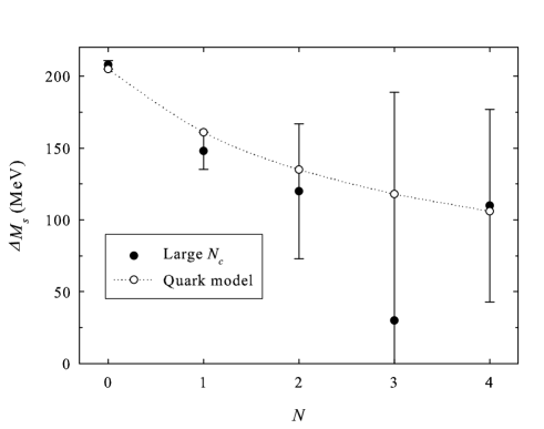
Figure 1: Plot of the results presented in Table 3. The quark model predictions for the mass shift $\Delta M_{s}$ (empty circles) are compared to the large $N_{c}$ data (full circles). A dotted line links the quark model points to guide the eye.

IV.2 The dependence on $N$

When $n_{s}=0$ or 3, the symmetry of the problem leads to a mass formula which depends on $N=N_{\xi}+N_{\eta}$ only, with $N_{\xi}$ and $N_{\eta}$ introduced in Sec. III.2. When $n_{s}=1$ or 2 however, this is not the case. In order to perform explicit calculations, we have assumed that $N$ is still a good quantum number to classify baryon states with one or two strange quarks. This assumption also ensures that the total parity remains $(-1)^{N}$ in a given band.

To quantitatively support the above considerations, we can now build a quantity to estimate the validity of this approximation for $n_{s}=1$ or 2. In this case, the general mass formula (17) must be used. It depends on the auxiliary fields, that we commonly denote here as $\varphi_{i}$, but also on $N_{\xi}$ and $N_{\eta}$. The value of $M(N_{\xi},N_{\eta},\varphi_{i})$, thus given by Eq. (17), can be computed once $\sigma$ and $m_{s}$ are fixed. We choose $\sigma=0.163$ GeV² and $m_{s}=0.243$ GeV as in the previous section. First, instead of $N_{\xi}$ and $N_{\eta}$, we work with the quantum numbers $N$ and $N^{\prime}=N_{\xi}$, that is to say with the mass formula $M(N^{\prime},N-N^{\prime},\varphi_{i})$ where $N^{\prime}=0,\dots,\,N$. Once $N$ and $N^{\prime}$ are fixed, standard numerical routines allow to minimize the mass with respect to the auxiliary fields. This leads to the optimal values $\varphi_{i,0}$ and finally to $M(N^{\prime},N-N^{\prime},\varphi_{i,0})$. Then, we define

$$\delta M(N)=\frac{\max\{M(N^{\prime},N-N^{\prime},\varphi_{i,0})\}-\min\{M(N^{\prime},N-N^{\prime},\varphi_{i,0})\}}{\left[\sum^{N}_{N^{\prime}=0}M(N^{\prime},N-N^{\prime},\varphi_{i,0})\right]/\left[N+1\right]},$$ (47)

where the maximal and minimal masses are chosen within the set of allowed $N^{\prime}$ for a given $N$. $\delta M$, which depends only on $m_{s}/\sqrt{\sigma}$, is a measure of the quality of $N$ as a good quantum number: The more $\delta M$ is small, the less the value of the mass at a given $N$ depends on the other quantum number $N^{\prime}$.

A plot of $\delta M$ versus $N$ is presented in Fig. 2 for the $nns$ and $nss$ baryons. By definition, $\delta M(0)=0$ since the only possibility is $N^{\prime}=0$ in this case. Then, it appears that $\delta M$ increases linearly for $N\geq 1$. Moreover, the values vary very slowly with $m_{s}/\sqrt{\sigma}$. The key point to observe in this graph is that $\delta M(N\leq 6)\lesssim$ 3%. As no experimental state such that $N>6$ has so far been observed, we can conclude that the mass formula obtained from the spinless Salpeter Hamiltonian (7) mainly depends on $N$: A change of $N^{\prime}$ at a given $N$ only causes a change of the mass which is lower than 3% in all the case that are relevant with regard to current experimental data.

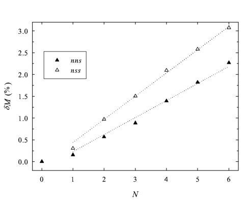
Figure 2: Plot of $\delta M$ ($\%$) versus $N$ for $nns$ baryons (full triangles) and for $nss$ baryons (empty triangles), with the parameters of Table 2. Linear fits for the $N>0$ points are plotted with a dotted line.

Let us note that the previous result is only strictly valid for the mass formula obtained from the Hamiltonian (14). When the eigenstates of the Hamiltonian (7) are computed in harmonic oscillator bases, it can be seen that these eigenstates contain components from different $N$ bands; thus $N$ is only an approximate good quantum number. Nevertheless, the band mixing is usually small and changes by less than 10% the mass of a state with a dominant component in a given band $N$.

IV.3 Regge trajectories

Since $N$ appears to be a relevant quantum number to classify light baryons with a good accuracy, it is of interest to study the predictions of large $N_{c}$ QCD and quark model regarding the Regge trajectories of nonstrange as well as of strange baryons. At the leading order in $N$, we actually expect that $M^{2}\propto N$. Indeed, formula (45) tells us that, at large $N$,

$$M^{2} \approx M^{2}_{0}+2M_{0}n_{s}\Delta M_{s}$$ (48)

$$= 2\pi\sigma(N+3)-\frac{4}{\sqrt{3}}\pi\sigma\alpha_{s}-3f\sigma+\left[6+\frac{f\sigma\beta}{\delta^{2}}\right]n_{s}m_{s}^{2}.$$

Our particular quark model thus states that baryons should follow Regge trajectories with a common slope, irrespective of the strangeness of the baryons. This feature has also been pointed out in other approaches based on the diquark-quark picture simobar ; SW . In Ref. lnc we have already shown that, for nonstrange baryons, $M^{2}_{0}$ was actually equal to $(N_{c}\,c_{1})^{2}$, this last quantity being the dominant term in the large $N_{c}$ mass formula. Moreover, following Ref. GM , the fitted values of $c_{1}$ does not change whether or not strange quarks are taken into account. Therefore, the Regge slope of strange and nonstrange baryons is also predicted to be independent of the strangeness in the $1/N_{c}$ expansion method.

However, the intercept depends on the number of strange quarks. Following the explicit formula (48), it logically increases for larger values of $n_{s}$ and $m_{s}$. Formally, the contribution of strange quarks to the intercept is given in the quark model by $\left.2M_{0}\Delta M_{s}\right|_{N=0}$, and in the large $1/N_{c}$ expansion by $2\,N_{c}\,c_{1}\,\left.\Delta M_{s}\right|_{N=0}$. Taking the values of $M_{0}$ and $c_{1}$ from Ref. lnc , and the values of $\Delta M_{s}$ found in this paper, both large $N_{c}$ QCD and quark model agree on the value of the intercept. The first method leads to $0.361\pm 0.005$ GeV², while the second one gives $0.355$ GeV².

The light baryon Regge trajectories are thus predicted to share a common slope, but we expect that they should be separated into parallel straight lines with an intercept depending on the strangeness. Unfortunately, too few experimental data are currently known at large excitation energies (large $N$) to check this picture. But, it could be used as an interesting tool to identify strange and nonstrange excited baryons in future experiments.

V Conclusion

The previous work establishing a connection between the quark model and the $1/N_{c}$ expansion method has been successfully extended to include strange baryons with nonzero mass $m_{s}$. A comparison between the SU(3)-breaking terms in the mass formula of the two approaches has been made and we found a good quantitative agreement. The comparison was possible through the introduction of a band quantum number $N$, customarily used in the baryon classification. While for nonstrange baryons $N$ appears straightforwardly, the inclusion of strange quarks with nonzero mass turned out to be more elaborate. However we have numerically proved that $N$ can be considered as a good quantum number in a realistic quark model with a $Y$-junction confinement by keeping terms up to order $m^{2}_{s}$ in the Taylor expansion.

- (1) C. Semay, F. Buisseret, N. Matagne, and Fl. Stancu, Phys. Rev. D 75, 096001 (2007).
- (2) N. Isgur and G. Karl, Phys. Rev. D 19, 2653 (1979).
- (3) G. ’t Hooft, Nucl. Phys. 72, 461 (1974).
- (4) E. Witten, Nucl. Phys. B 160, 57 (1979).
- (5) J. L. Gervais and B. Sakita, Phys. Rev. Lett. 52, 87 (1984); Phys. Rev. D 30, 1795 (1984).
- (6) R. Dashen and A. V. Manohar, Phys. Lett. B 315, 425 (1993); ibid, 438 (1993) .
- (7) R. Dashen, E. Jenkins, and A. V. Manohar, Phys. Rev. D 49, 4713 (1994).
- (8) R. Dashen, E. Jenkins, and A. V. Manohar, Phys. Rev. D 51, 3697 (1995).
- (9) E. Jenkins, Ann. Rev. Nucl. Part. Sci. 48, 81 (1998).
- (10) E. Jenkins, hep-ph/0111338.
- (11) N. Matagne and Fl. Stancu, Phys. Rev. D 74, 034014 (2006).
- (12) J. L. Goity, C. L. Schat, and N. N. Scoccola, Phys. Rev. D 66, 114014 (2002).
- (13) J. L. Goity, C. Schat, and N. N. Scoccola, Phys. Lett. B 564, 83 (2003).
- (14) N. Matagne and Fl. Stancu, Phys. Rev. D 71, 014010 (2005).
- (15) J. L. Goity and N. Matagne, arXiv:0705.3055.
- (16) P. Stassart and Fl. Stancu, Phys. Lett. B 269, 243 (1991).
- (17) P. Stassart and Fl. Stancu, Z. Phys. A 359, 321 (1997).
- (18) J. Carlson, J. Kogut, and V. R. Pandharipande, Phys. Rev. D 27, 233 (1983).
- (19) Y. Koma, E.-M. Ilgenfritz, T. Suzuki, and H. Toki, Phys. Rev. D 64, 014015 (2001).
- (20) B. Silvestre-Brac, C. Semay, I. M. Narodetskii, and A. I. Veselov, Eur. Phys. J. C 32, 385 (2004).
- (21) A. M. Badalian and V. L. Morgunov, Phys. Rev. D 60, 116008 (1999); A. M. Badalian and B. L. G. Bakker, Phys. Rev. D 66, 034025 (2002).
- (22) G. S. Bali, Phys. Rep. 343, 1 (2001).
- (23) Yu. A. Simonov, Phys. Lett. B 515, 137 (2001); F. Buisseret and C. Semay, Phys. Rev. D 71, 034019 (2005).
- (24) A. Di Giacomo and H. Panagopoulos, Phys. Lett. B 285, 133 (1992).
- (25) A. Di Giacomo and Yu. A. Simonov, Phys. Lett. B 595, 368 (2004).
- (26) C. Semay, B. Silvestre-Brac, and I. M. Narodetskii, Phys. Rev. D 69, 014003 (2004).
- (27) F. Buisseret and C. Semay, Phys. Rev. D 73, 114011 (2006).
- (28) F. Buisseret and V. Mathieu, Eur. Phys. J. A 29, 343 (2006).
- (29) F. Buisseret, Phys. Rev. C 76, 025206 (2007).
- (30) W.-M. Yao et al., J. Phys. G 33, 1 (2006).
- (31) W. Lucha, F. Schöberl, and D. Gromes, Phys. Rep. 200, 127 (1991).
- (32) Yu. A. Simonov, Phys. Lett. B 228, 413 (1989).
- (33) A. Selem and F. Wilczek, hep-ph/0602128.