Modeling Crowd Turbulence by Many-Particle Simulations

Abstract

A recent study [D. Helbing, A. Johansson and H. Z. Al-Abideen, Phys. Rev. E 75, 046109 (2007)] has revealed a “turbulent” state of pedestrian flows, which is characterized by sudden displacements and causes the falling and trampling of people. However, turbulent crowd motion is not reproduced well by current many-particle models due to their insufficient representation of the local interactions in areas of extreme densities. In this contribution, we extend the repulsive force term of the social force model to reproduce crowd turbulence. We perform numerical simulations of pedestrians moving through a bottleneck area with this new model. The transitions from laminar to stop-and-go and turbulent flows are observed. The empirical features characterizing crowd turbulence, such as the structure function and the probability density function of velocity increments are reproduced well, i.e. they are well compatible with an analysis of video data during the annual Muslim pilgrimage.

I Introduction

Pedestrian dynamicscrowdturbulence ; PREsfm ; stillPhD has been described by physicists through various macroscopic and microscopic models. Macroscopic models, predominantly fluid-dynamic models fluidRev ; fluidTRB , have the advantage of describing the large-scale dynamics of crowds, especially depicting intermittent flows and stop-and-go flows. These features are basically understood as the effect of a hybrid continuity equation PRLbottleneck with two regimes: forward pedestrian motion and backward gap propagation. Details of pedestrian interactions are neglected in these models. In contrast, microscopic models can be used to describe the details of pedestrian behavior. Previously proposed pedestrian models include many-particle force modelsPREcfm ; panic , CA models CABurs ; CAMura and others, e.g. multi-agent approaches AgentM , which have received an increasing attention among physicists in the past. In recent years, the interest has turned to empirical or experimental studies Exp1 ; Exp2 ; Exp3 ; Exp4 ; Exp5 ; Exp6 ; transci of pedestrian flows based on video analysis crowdturbulence ; VideoAnalysis ; Exp5 ; Exp2 ; KerridgeEmpirical . This has contributed to the calibration of current models calibration ; hoogendoornPED and the discovery of new phenomena such as crowd turbulence crowdturbulence , which can help to understand many crowd disasters.

Turbulent motion of pedestrians occurs, when the crowd is extremely compressed, and people attempt to gain space by pushing others, which leads to irregular displacements, or even the falling of people. If the fallen pedestrians do not manage to stand up quickly enough, they will become obstacles and cause others to fall as well. Such dynamics can eventually spread over a large area and result in a crowd disaster.

However, crowd turbulence is not well reproduced and understood by pedestrian models yet, which challenges current many-particle models. Their shortcoming is due to the underestimation of the local interactions triggered by high densities. In the following sections, we will extend the repulsive force of the social force model PREsfm ; panic ; transci , which has successfully depicted many observed self-organized phenomena, such as lane formation in counter flows and oscillatory flows at bottlenecks sfmBook .

II Model of Crowd Turbulence

Previous empirical studiescrowdturbulence ; Fruin have revealed that people are involuntarily moved when they are densely packed, and as a consequence, the interactions increases in areas of extreme densities, which leads to an instability of pedestrian flows. When the average density is increasing, sudden transitions from laminar to stop-and-go and turbulent flows are observed. Moreover, the average flow does not reach zero. We will now show how the turbulent flows can be modeled, by a small extension of the social force modelPREsfm ; panic ; transci . What we do is to add an extra term to the repulsive force, and show how this will give qualitatatively different dynamics, leading to turbulent flows.

The social force model assumes that a pedestrian $i$ tries to move in a desired direction $\vec{e}_{i}$ with desired speed $v_{i}^{0}$, and adapt the actual velocity $\vec{v}_{i}$ to the desired velocity $v_{i}^{0}\vec{e}_{i}$ within the relaxation time $\tau$. The velocity $\vec{v}_{i}=d\vec{r}_{i}/dt$, i.e. the temporal change of the position $\vec{r}_{i}$ is also affected by repulsive forces.

The social force model is given by

$$m_{i}\frac{d\vec{v_{i}}(t)}{dt}=\vec{f_{i}}(t),$$ (1)

where $\vec{f}_{i}(t)$ is the acceleration force of pedestrian $i$

$$\vec{f}_{i}(t)=m_{i}\frac{1}{\tau}(v_{i}^{0}\vec{e}_{i}-\vec{v}_{i})+\sum_{j(\neq{i})}\vec{f}_{ij}(t).$$ (2)

The term $\vec{f}_{ij}(t)$ denotes the repulsive force, which represents both the attempt of pedestrian $i$ to keep a certain safety distance to other pedestrians $j$ and the desire to gain more space in very crowded situations.

Instead of introducing an additional force term, one may reflect the desire to gain more space under crowded conditions, by a local interaction range in the repulsive pedestrian force $\vec{f}_{ij}$, which is proposed as follows,

$$\vec{f_{ij}}=F\Theta(\varphi_{ij})\exp[-d_{ij}/D_{0}+(D_{1}/d_{ij})^{k}]\vec{e}_{ij},$$ (3)

where $F$ is the maximum repulsive force ( assuming there is no overlapping/compression ); $d_{ij}$ is the distance between center of masses of pedestrians; $k$, $D_{0}$, and $D_{1}$ are constants; $\vec{e}_{ij}$ is the normalized vector pointing from pedestrian $j$ to pedestrian $i$, $\varphi_{ij}$ is the angle between $\vec{e}_{ji}$ and the desired walking direction $\vec{e}_{i}$ of pedestrian $i$, i.e. $\cos(\varphi_{ij})=\vec{e}_{i}\cdot\vec{e}_{ji}$.

In normal situations, the function $\Theta(\varphi_{ij})$ reflects the fact that pedestrians react much stronger to what happens in front of them, and it has been suggested sfmBook to have the form,

$$\Theta(\varphi)=\Big{(}\lambda+(1-\lambda)\frac{1+\cos(\varphi)}{2}\Big{)}.$$ (4)

Also note that when $d_{ij}$ is very small, i.e., people are squeezed, the repulsive force will increase greatly, which reflects the strong reactions of those located in extremely dense areas.

In the original social force model, the second repulsion term $kg(r_{ij}-d_{ij})$ panic reflects the physical contacts of pedestrians, which will separate pedestrians, when collisions occur. Here k is a constant, and function g(x) is zero, if pedestrians do not touch each other, otherwise it is equal to the argument $x$. In highly dense areas, the speeds of pedestrians are very low, so the small fluctuations of $d_{ij}$ may not lead to sufficient forces for the occurrence of turbulence, since this repulsive force is increased linearly. Suppose that pedestrian $i$ is located in an extremely dense area. For the extended model, the small fluctuations of $d_{ij}$ will change the repulsive forces greatly, and lead to sudden involuntary displacements. With the influence of such strong reactions, the motion of pedestrians near $i$ will be affected, and will further spread the irregular displacements to a larger area. Thus the turbulent motion of pedestrians will be triggered.

III Results and Discussion

Numerical simulations (supplementary videos supplement ) will now be carried out, of a crowd going through a bottleneck. The simulations will be performed with the extended-social-force model described in Sec. II.

In our simulations, the desired speeds $v^{0}$ are assumed to be Gaussian distributed with the mean value $v^{0}=1.34m/s$ and the standard deviation $0.26m/s$ Param1 ; Param2 ; Param3 . The relaxation time, $\tau$ is set to $0.5s$. The average mass of a pedestrian is set to $60kg$ with a standard deviation of $10kg$. Assuming that pedestrians have a strong desire to gain more space in dense areas, the maximum repulsive force $F$ is set to $160N$. Note that, when pedestrians are compressed, the maximum force can be significantly larger than F. The other parameters are set to, $\lambda=0.25$, $k=2$, $D_{0}=0.31$ and $D_{1}=0.45$.

The bottleneck area (see Fig. 1) contains two pedestrian sources, $A$ and $B$, where $A$ denotes those walking from left to right, while $B$ represents those walking from the bottom, and then turn right to join those coming from left. These two sources give an increasing number of pedestrians in time, since we use both pedestrian sorces as well as periodic boundary conditions. With this scheme we can see how the transition from laminar to turbulent flow occur when the density is growing. The whole area is $40m\times 20m$. The reason for this setup, is to get a situation that is comparable to the one in the empirical studycrowdturbulence .

The preferred direction is defined as follows:̱ If the vertical position of a pedestrian is above the corner, he/she will walk in the right direction. Otherwise, he/she will first walk upwards until he/she is above the corner, and then turn to the right and keep walking straight ahead.

Note that interactions increase greatly when those two crowds intersect, especially in high density situations.

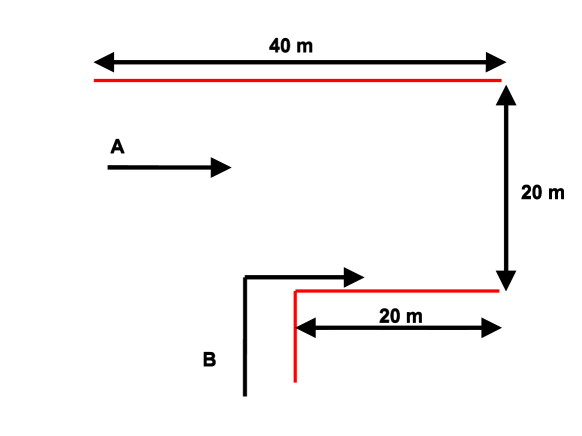
Figure 1: (Color online) The bottleneck area of the simulation. Two groups of people set out respectively from A and B, and intersect, causing pedestrians to be highly compressed, which eventually results in turbulent flows.

The “Crowd pressure”crowdturbulence , reflecting the irregular/chaotic motion of people, is given by

$$p=\rho_{i}\mbox{Var}(\vec{v}_{i}),$$ (5)

where $\mbox{Var}(\vec{v}_{i})$ is the local velocity variance. The local density $\rho_{i}$,

$$\rho_{i}=\sum_{j}\frac{1}{\pi R^{2}}exp(-\|\vec{r_{j}}(t)-\vec{r_{i}}(t)\|^{2}/R^{2}).$$ (6)

$R$ is a parameter reflecting the range of smoothing. For further aspects regarding the definition of the local density and pressure, see Ref.crowdturbulence .

The pressure stays low during an increasing density, until a point where the pressure suddenly peaks, which leads to the turbulent crowd motion (see Fig. 2).

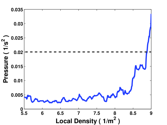
Figure 2: (Color online) The crowd pressure as a function of local density. The turbulence starts when the pressure exceeds a value of $0.02/s^{2}$crowdturbulence .

The fundamental diagram (see Fig. 3) demonstrates the effect of the extended repulsive force term. One can clearly see the difference at the tail of the curve, where the flow remains finite with the increase of local density. Note that the flow here is not reduced to zero, even if the density is very high due to the strong interactions within the crowd, which will prevent people from stopping. If the flow is reduced to zero, which means all the people stop moving, then there is no turbulence. Therefore it is essential to have nonvanishing flow for high densities. This is compatible with the empirical study crowdturbulence . Note that, at this point, the flow is no longer laminar. Therefore, the strong interactions between pedestrians are potentially more dangerous for the crowd. The motion of pedestrians become turbulent, and people are pushed into all possible directions. As people are pushed by those behind, the fallen people will be trampled, if they do not get back on their feet quickly enough. However, in our simulations, we assume that pedestrians will never fall, since we are focussing on the dynamics of the crowd during a high level of crowdedness. These conditions can potentially lead to an accident, but we do not focus on the dynamics of the accident itself.

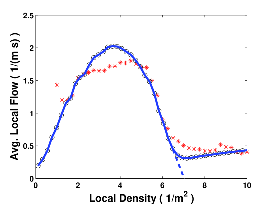
Figure 3: (Color online) The average of the local flow crowdturbulence as a function of the local density. The empirical data is represented by stars and the simulation results are represented by circles connected by a solid line. The dashed line shows the fundamental diagram, from the original social force model.

With the increment of density, the pedestrian flow suddenly turns into stop-and-go flow (see Fig. 4), which is characterized by temporarily interrupted and longitudinally unstable flow. This phenomenon is also predicted by a recent theoretical approach PRLbottleneck , which suggests that intermittent flows at bottlenecks can be triggered when the inflow exceeds the outflow.

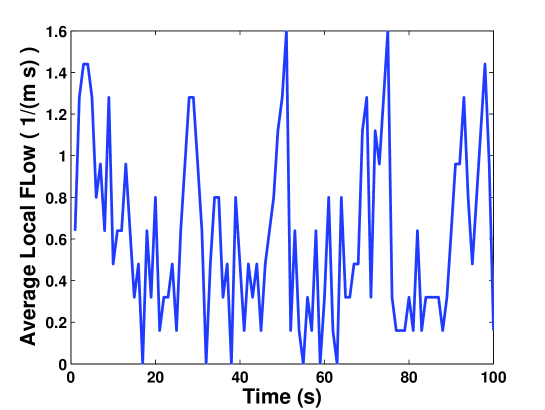
Figure 4: (Color online) Simulation results. During high crowd densities, the smooth, laminar flow will turn into stop-and-go flow. Here the average density is $4.3/m^{2}$.

Further increment of the density will lead to turbulent flows. Figure 5(a) shows a typical trajectory of the turbulent motion from our simulations. We can see that, first, the curve is smooth, which represents a laminar flow, then suddenly, vibrations occur due to the turbulence. Also, note that the pedestrian is sometimes even pushed backwards. The turbulent motion does not vanish until an individual walks out of the extremely dense central area, where the two streams intersect. Figure 5(b) is an example of the temporal evolution of an individual’s velocity components $v_{y}$ and $v_{x}$. One can clearly see the irregular motion into all directions. Although no large eddies are observed, as in turbulent fluids, there is still an analogy to the turbulence of the currency exchange market exchangemarket . This can be characterized by the probability density function of velocity increments and the so-called structure function, Eq. 8.

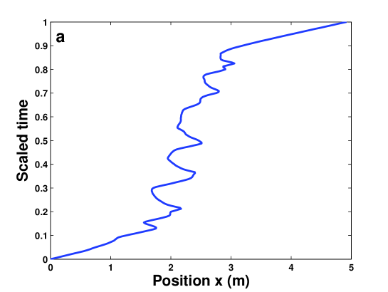
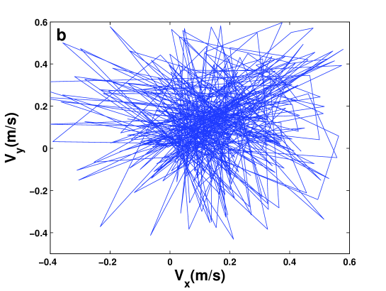
Figure 5: (Color online) (a) A representative pedestrian trajectory in laminar and turbulent flow. (b) An example of velocity components in the turbulent motion. Here the average density is $9.0/m^{2}$.

The shape of the probability density function of velocity increment is a typical indicator for turbulence, if the time shift $\tau^{\prime}$ is small enough, and is given by

$$v_{x}^{\tau^{\prime}}=v_{x}(\vec{r},t+\tau^{\prime})-v_{x}(\vec{r},t).$$ (7)

The structure function,

$$S(\bigtriangleup\vec{r})=\langle\|\vec{v}(\vec{r}+\bigtriangleup\vec{r},t)-\vec{v}(\vec{r})\|^{2}\rangle_{\vec{r},t},$$ (8)

reflects the dependence of the relative speed on the distance.

We find that the probability functions of velocity increment is sharply peaked for turbulence, while it is parabolic-like for laminar flow (see Fig. 6), when the time shift $\tau^{\prime}$ is small enough. The structure function has a slope of $2.0$, when the distance is small, while at large steps, the slope turns to $0.18$ due to the increased interactions in crowded regions. Both of the functions are compatible to the analysis of the video recordings of the Jamarat Bridgecrowdturbulence .

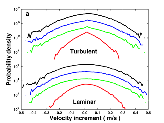
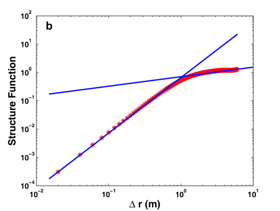
Figure 6: (Color online) (a) the probability density function of the velocity increment in the laminar and the turbulent region, determined over many locations $\vec{r}$ for $R=\sqrt{10/\rho}$ and $\tau^{\prime}=2s$( black curves, top ), $\tau^{\prime}=1s$( blue curves, second ), $\tau^{\prime}=0.5s$( green curves, third ), and $\tau^{\prime}=0.05s$( red curves, bottom ). For the clarity of the presentation, the curves are shifted in the vertical direction. The non-parabolic, peaked curve for small values of $\tau^{\prime}$ distinguishes turbulence from laminar flows. (b) The log-log plot of the structure function for crowd turbulence. The average density here is $9.0/m^{2}.$

IV Summary and Outlook

In summary, an added social force component, reflecting the strong interactions in the extremely crowded areas is proposed for the simulation of crowd turbulence, which questions current many-particle models. The transition from laminar to stop-and-go and turbulent flows is observed in the simulations. The fundamental diagram is reproduced and demonstrates the effects of the extended repulsive forces at highly dense situations, i.e. the average local flow is not reduced to zero. A typical turbulent trajectory and velocity components are presented. Functions like the probability density function of velocity increment and the structure function, characterizing the features of turbulence are simulated, and the results are compatible to the empirical studies.