Controllability of Quantum Systems on the Lie Group $SU(1,1)$

Abstract

This paper examines the controllability for quantum control systems with $SU(1,1)$ dynamical symmetry, namely, the ability to use some electromagnetic field to redirect the quantum system toward a desired evolution. The problem is formalized as the control of a right invariant bilinear system evolving on the Lie group $SU(1,1)$ of two dimensional special pseudo-unitary matrices. It is proved that the elliptic condition of the total Hamiltonian is both sufficient and necessary for the controllability. Conditions are also given for small time local controllability and strong controllability. The results obtained are also valid for the control systems on the Lie groups $SO(2,1)$ and $SL(2,\mathbb{R})$.

I Introduction

Controllability is a fundamental problem in the control theory with respect to both classical Sussmann (1972); R.W.Brockket (1972); Jurdjevic and Sussman (1972); Sussmann (1983) and quantum Huang et al. (1983); Ramakrishna et al. (1995); Tarn et al. (2000); D’Alessandro (2000); Schirmer et al. (2001); Lan et al. (2005); Wu et al. (2006a) mechanical system. In the past decades, sufficient conditions Jurdjevic and Sussman (1972); Huang et al. (1983); Ramakrishna et al. (1995); Lan et al. (2005); Wu et al. (2006a) have been established via algebraic methods for systems evolving on manifolds or Lie groups. However, most of these conditions are not necessary, especially for the systems on noncompact Lie groupsJurdjevic and Sussman (1972).

The main purpose of this article is to establish a sufficient and necessary condition that examines the controllability of the quantum systems whose propagators evolve on the noncompact Lie group $SU(1,1)$, which describes the dynamical symmetry of many important physical possesses, e.g., the downconversion process Puri (2001); Gerry and Vrscay (1989), the Bose-Einstein condensation Gortel and Turski (1991), the spin wave transition in solid-state physics Bose (1985), the evolution in free space Agarwal and Banerji (2001).

The problem is investigated by considering the following right invariant bilinear system on the Lie group $SU(1,1)$

$$\dot{X}(t)=\left[A+\sum\limits_{l=1}^{r}u_{l}(t)B_{l}\right]X(t),X(0)=I_{2},$$ (1)

where $u_{l}(t)$ belong to some admissible control set $\mathcal{U}$, which consists of functions defined on $\mathbb{R}^{+}=[0,\infty)$. The drift term $A$ and the control terms $B_{1}$, $B_{2}$, $\cdots$, $B_{r}$ are elements of the Lie algebra $su(1,1)$, where $B_{1}$, $B_{2}$, $\cdots$, $B_{r}$ are assumed to be linearly independent with respect to real coefficients. The state, $X(t)$, is a two-dimensional complex pseudo-unitary matrix in the form of

$$\left(\begin{array}[]{cc}a&b\\ \bar{b}&\bar{a}\\ \end{array}\right),~{}~{}~{}~{}~{}|a|^{2}-|b|^{2}=1,$$ (2)

where $\bar{a}$ represents the complex conjugate of $a$. Since $SU(1,1)$ is homomorphic to $SO(2,1)$ and isomorphic to $SL(2,\mathbb{R})$ respectively, the results obtained in this paper are still valid for the systems on these two Lie groups.

For a driftless system varying on the noncompact Lie group, it was shown in Jurdjevic and Sussman (1972) that the system is controllable when there exists a constant control such that the state trajectory is periodic. Applied to the quantum system evolving on $SU(1,1)$, it can be concluded that the system is controllable if the total Hamiltonian (including the internal Hamiltonian and the interaction Hamiltonian) of the system can be adjusted to be elliptic. In Wu et al. (2006b), this sufficient condition was extended to bounded controls, algorithms were given accordingly to design control laws to achieve desired evolutions. In this paper, this condition is proven to be necessary for the single input case, which can be directly used to judge whether one can find a “magnetic field” to induce a desired transition between two arbitrary $SU(1,1)$ coherent states, which are of particular importance in quantum optics Gerry (1985); Walls (1983).

The paper is organized as follows. Section II presents preliminaries to be used in the rest of this paper. Subsection II.1 describes the systems to be considered in mathematical terms of right invariant bilinear control systems that evolve on the noncompact Lie group $SU(1,1)$. Subsection II.2 introduces necessary definitions for the system controllability. Section III contains the main results on the system controllability. In Subsection III.1, we present some properties of Lie algebra $su(1,1)$ that will be useful for studying the system controllability. In Subsection III.2, a sufficient and necessary condition that examines the controllability is established for the single input case, showing that the controllability of such quantum systems can be completely determined by finding a constant control that adjusts the total Hamiltonian of the undergoing system to be elliptic, or not. Properties of the strong controllability and small time local controllability are discussed in the subsequence as well. Controllability properties for the multi-input case is considered in Subsection III.3. In Section IV, we discuss the relationship between systems evolving on $SO(2,1)$, $SL(2,\mathbb{R})$ and $SU(1,1)$ and show that the result obtained are still valid for the system evolving on these noncompact Lie groups. Interpretations are then provided for the criteria obtained based on the topology of $SO(2,1)$. Illustrative examples are elaborated in Section VI. Finally, conclusions are drawn in section VI.

II Preliminaries

In this section, we present preliminaries which will be used in this paper.

II.1 Quantum Control Systems on $SU(1,1)$

The time evolution of a controlled quantum system is determined through the Schrödinger equation

$$i\hbar\frac{d}{dt}\psi(t)=\left[H_{0}+\sum_{l=1}^{r}u_{l}(t)H_{l}\right]\psi(t),~{}\psi(0)=\psi_{0},$$ (3)

where the wave function $\psi(t)$ describes the state of the system in an appropriate Hilbert space $\mathcal{H}$. The Hermitian operators $H_{0}$ and $H_{l}~{}(l=1,2,\cdots,r)$ are referred to as the internal and interaction Hamiltonians respectively. The scalars $u_{l}(t)~{}(l=1,2,\cdots,r)$ represent some adjustable classical fields coupled to the system, which are used to control the evolution of the system.

In this paper, we study the class of quantum systems evolving on the noncompact Lie group $SU(1,1)$, whose internal and interaction Hamiltonians can be expressed as linear combinations of the operators $K_{x}$, $K_{y}$ and $K_{z}$, which satisfy the following commutation relations

$$[K_{x},K_{y}]=-iK_{z},~{}[K_{y},K_{z}]=iK_{x},~{}[K_{z},K_{x}]=iK_{y},$$ (4)

i.e., closed as an $su(1,1)$ Lie algebra. According to the group representation theory Vilenkin and Klimyk (1991), $H_{0}$ and $H_{l}~{}(l=1,2,\cdots,r)$ are all operators on an infinite dimensional Hilbert space $\mathcal{H}$ because $su(1,1)$ is noncompact (see Example 1).

Let $U(t)$ be the evolution operator (or propagator) that transforms the system state from the initial $\psi(0)$ to $\psi(t)$, i.e., $\psi(t)=U(t)\psi(0)$. Then, from (3), by setting $\hbar=1$ and $\bar{H}_{l}=-iH_{l}~{}(l=0,1,\cdots,r)$, we can obtain that

$$\dot{U}(t)=\left[\bar{H}_{0}+\sum_{l=1}^{r}u_{l}(t)\bar{H}_{l}\right]U(t),~{}U(0)=I,$$ (5)

where $I$ is the identity operator on $\mathcal{H}$. The evolution operator $U(t)$ can be treated as an infinite dimensional matrix since it acts on the infinite dimensional states space. It is inconvenient to study the controllability properties of such infinite-dimensional systems directly. Nevertheless, since all faithful representations are algebraically isomorphic on which the system controllability property does not rely, one can always focus the study on the equivalent system (1) evolving on the Lie group $SU(1,1)$ of pseudo-unitary matrices, where $A$ and $B_{l}$ can be written down as linear combinations of

$$\begin{array}[]{l}\bar{K}_{x}=\frac{1}{2}\sigma_{y}=\frac{1}{2}\left(\begin{array}[]{cc}0&-i\\ i&0\\ \end{array}\right),~{}~{}\bar{K}_{y}=-\frac{1}{2}\sigma_{x}=\frac{1}{2}\left(\begin{array}[]{cc}0&-1\\ -1&0\\ \end{array}\right),~{}~{}\bar{K}_{z}=-\frac{i}{2}\sigma_{z}=\frac{1}{2}\left(\begin{array}[]{cc}-i&0\\ 0&i\\ \end{array}\right),\end{array}$$ (6)

where $\sigma_{x,y,z}$ are Pauli matrices. The matrices $\bar{K}_{x}$, $\bar{K}_{y}$ and $\bar{K}_{z}$ are non-unitary representation of the operators $K_{x}$, $K_{y}$ and $K_{z}$, and one can verify that $\bar{K}_{x}$, $\bar{K}_{y}$ and $\bar{K}_{z}$ satisfy

$$[\bar{K}_{x},\bar{K}_{y}]=-\bar{K}_{z},~{}[\bar{K}_{y},\bar{K}_{z}]=\bar{K}_{x},~{}[\bar{K}_{z},\bar{K}_{x}]=\bar{K}_{y}.$$ (7)

$\bar{K}_{x}$, $\bar{K}_{y}$ and $\bar{K}_{z}$ form a normalized orthonormal basis of the Lie algebra $su(1,1)$ with respect to the inner product $\left<\cdot,\cdot\right>$ defined by

$$\left<M,~{}N\right>=2~{}\mbox{Tr}(MN^{\dagger}),$$ (8)

where $N^{\dagger}$ denotes the Hermitian conjugation of $N$. As a result, any given element $M$ in $su(1,1)$ can be expressed in the following way

$$M=\left<M,\bar{K}_{x}\right>\bar{K}_{x}+\left<M,\bar{K}_{y}\right>\bar{K}_{y}+\left<M,\bar{K}_{z}\right>\bar{K}_{z}.$$ (9)

II.2 Controllability and the Reachable Sets

To define the controllability of system (1), the following reachable sets started from the identity $I_{2}$ are useful,

1. $R(t)=\{X_{f}|\exists~{}u,s.t.,X(0)=I_{2},X(t)=X_{f}\}$, i.e., the set of all the possible values for state $X(t)$ at time $t$.

2. $R(\cup{T})=\bigcup_{0\leq{t}\leq{T}}R(t)$ ($R(\cup{\infty})=\bigcup_{0\leq{t}<\infty}R(t)$), i.e., the set of all the possible states within time $T$ ($\infty$).

3. $R(\cap{T})=\bigcap_{0<{t}\leq{T}}R(t)$ ($R(\cap{\infty})=\bigcap_{0<{t}<\infty}R(t)$), i.e., the set of all values for state $X(t)$ that can be achieved at any time within $T$ ($\infty$).

With the reachable sets defined above, controllability of the system (1) can be defined as follows.

Definition 1: System (1) is said to be controllable on $SU(1,1)$ if $R(\cup{\infty})=SU(1,1)$, strongly controllable on $SU(1,1)$ if $R(\cap{\infty})=SU(1,1)$, and small time local controllable on $SU(1,1)$ if $I_{2}$ is an interior point of $R(t)$ for any $t>0$.

Apparently, system (1) is both controllable and small time local controllable if it is strongly controllable. The right invariant property indicates that the controllability properties of system (1) is independent of the system initial condition.

Before discussing the controllability of system (1), we introduce the following three Lie algebras.

1. $\mathcal{L}$ is the Lie algebra generated by $\{A,B_{1},B_{2},\cdots,B_{r}\}$, and $e^{\mathcal{L}}$ is the connected Lie subgroup of $SU(1,1)$ exponentiated by $\mathcal{L}$.

2. $\mathcal{L}_{0}$ is the maximal ideal in $\mathcal{L}$ generated by $\{B_{1},B_{2},\cdots,B_{r}\}$, and $e^{\mathcal{L}_{0}}$ is the connected Lie subgroup of $SU(1,1)$ exponentiated by $\mathcal{L}_{0}$.

3. $\mathcal{B}$ is the algebra generated by $\{B_{1},B_{2},\cdots,B_{r}\}$, and $e^{\mathcal{B}}$ is the connected Lie subgroup of $SU(1,1)$ exponentiated by $\mathcal{B}$.

Clearly, $R(\cup{\infty}){\subseteq}e^{\mathcal{L}}$, which implies that $e^{\mathcal{L}}$ must equal $SU(1,1)$ if system (1) is controllable. $\mathcal{L}_{0}$ has co-dimension 0 or 1 in $\mathcal{L}$ depending on whether $A$ is an element of $\mathcal{L}_{0}$ or not.

III Controllability

In this section, the results on the controllability of the systems with respect to both single-input and multi-input cases will be presented. For that purpose, the following properties of Lie algebra $su(1,1)$ will be very useful.

III.1 Properties of Lie Algebra $su(1,1)$

Definition 2: An $su(1,1)$ element $M$ (as well as its exponential $\exp(tM)$) is called elliptic (hyperbolic, parabolic) if $\left<M,M^{\dagger}\right>$ is negative (positive, zero).

Lemma III.1

The commutator $[M,N]$ is elliptic (parabolic, or hyperbolic) if and only if $\left<M,N^{{\dagger}}\right>^{2}-\left<N,N^{{\dagger}}\right>\left<M,M^{{\dagger}}\right><0$ ($=0$, or $>0$).

Proof:  Since $\bar{K}_{x}$, $\bar{K}_{y}$ and $\bar{K}_{z}$ span the Lie algebra $su(1,1)$, we can write

$$M=m_{1}\bar{K}_{x}+m_{2}\bar{K}_{y}+m_{3}\bar{K}_{z},$$ (10)

and

$$N=n_{1}\bar{K}_{x}+n_{2}\bar{K}_{y}+n_{3}\bar{K}_{z},$$ (11)

where the coefficients $m_{l}$ and $n_{l}$ are real numbers. Making use of the commutation relations given in (4), we have

$$[M,N]=(m_{2}n_{3}-m_{3}n_{2})\bar{K}_{x}+(m_{3}n_{1}-m_{1}n_{3})\bar{K}_{y}-(m_{1}n_{2}-m_{2}n_{1})\bar{K}_{z}.$$ (12)

A simple computation yields that

$$\begin{array}[]{l}\left<M,M^{{\dagger}}\right>=m_{1}^{2}+m_{2}^{2}-m_{3}^{2},~{}~{}\left<N,N^{{\dagger}}\right>=n_{1}^{2}+n_{2}^{2}-n_{3}^{2},~{}~{}\left<M,N^{{\dagger}}\right>=m_{1}n_{1}+m_{2}n_{2}-m_{3}n_{3},\end{array}$$ (13)

and

$$\left<[M,N],[M,N]^{\dagger}\right>=(m_{2}n_{3}-m_{3}n_{2})^{2}+(m_{3}n_{1}-m_{1}n_{3})^{2}-(m_{1}n_{2}-m_{2}n_{1})^{2}.$$ (14)

Comparison of (13) and (14) gives

$$\left<[M,N],[M,N]^{{\dagger}}\right>=\left<M,N^{{\dagger}}\right>^{2}-\left<N,N^{{\dagger}}\right>\left<M,M^{{\dagger}}\right>.$$ (15)

The statement of the Lemma follows immediately from the above equation.                                     $\square$

Lemma III.2

Given any two linearly independent elements $M$ and $N$ in $su(1,1)$, $M$, $N$ and $[M,N]$ are linearly independent if and only if $[M,N]$ is not parabolic.

Proof:  From (10)-(12), it can be concluded that $M$, $N$ and $[M,N]$ are linearly independent if and only if

$$\left|\begin{array}[]{ccc}m_{1}&n_{1}&m_{2}n_{3}-m_{3}n_{2}\\ m_{2}&n_{2}&m_{3}n_{1}-m_{1}n_{3}\\ m_{3}&n_{3}&-(m_{1}n_{2}-m_{2}n_{1})\\ \end{array}\right|\neq 0,$$ (16)

or equivalently

$$(m_{2}n_{3}-m_{3}n_{2})^{2}+(m_{3}n_{1}-m_{1}n_{3})^{2}-(m_{1}n_{2}-m_{2}n_{1})^{2}\neq 0,$$ (17)

i.e., $\left<[M,N],[M,N]^{\dagger}\right>\neq 0$. It immediately follows from Eq.(15) that $M$, $N$ and $[M,N]$ are linearly independent if and only if $[M,N]$ is not parabolic.                $\square$

Lemma III.3

Assume that $M$ and $N$ are linearly independent elements of $su(1,1)$ and the set $\{u\in\mathbb{R}|\left<M\right.+uN,M^{{\dagger}}+\left.uN^{{\dagger}}\right><0\}$ is empty, then $M+uN$ is hyperbolic for each $u\in\mathbb{R}$ if the commutator $[M,N]$ is not parabolic.

Proof:  Because the set $\left\{u\in\mathbb{R}|\left<M+uN,M^{{\dagger}}+uN^{{\dagger}}\right><0\right\}$ is empty, we have

$$\left<M+uN,M^{{\dagger}}+uN^{{\dagger}}\right>\geq 0,~{}\forall~{}u\in\mathbb{R},$$ (18)

or equivalently

$$\left<N,N^{{\dagger}}\right>u^{2}+2\left<M,N^{{\dagger}}\right>u+\left<M,M^{{\dagger}}\right>\geq 0,~{}\forall~{}u\in\mathbb{R}.$$ (19)

The case that $\left<N,N^{{\dagger}}\right><0$ can be directly excluded from (19). For the case when $\left<N,N^{{\dagger}}\right>=0$, from (19) we have $\left<M,N^{{\dagger}}\right>=0$. Then, combined with (15), $[M,N]$ must be parabolic, which contradicts with the assumption. For the case when $\left<N,N^{{\dagger}}\right>>0$, (19) holds if and only if $\left<M,N^{{\dagger}}\right>^{2}-\left<N,N^{{\dagger}}\right>\left<M,M^{{\dagger}}\right>\leq 0$. If $[M,N]$ is not parabolic, the previous inequality can be rewritten as $\left<M,N^{{\dagger}}\right>^{2}-\left<N,N^{{\dagger}}\right>\left<M,M^{{\dagger}}\right><0$, which implies that $M+uN$ is hyperbolic for each $u\in\mathbb{R}$.                $\square$

III.2 Controllability for Single-Input Case

Assume that there is only one control in (1), i.e.,

$$\dot{X}(t)=[A+u(t)B]X(t),~{}X(0)=I_{2}.$$ (20)

If $A$ and $B$ are linearly independent, i.e., they commute with each other, the solution of system (20) can be expressed as

$$X(t)=\exp\left[At+B\int_{0}^{t}u(\tau)d\tau\right].$$ (21)

Accordingly, the reachable set $R(\cup{\infty}){\subseteq}e^{\mathcal{L}}=\{X|X=\exp(Bs),s\in\mathbb{R}\}$ is a proper subgroup of $SU(1,1)$, which can never fill up $SU(1,1)$. Thus, system (20) is always uncontrollable in this case. In the following, we only consider the nontrivial case when $A$ and $B$ are linearly independent.

For systems evolving on the compact Lie group $SU(2)$, it has been shown in D’Alessandro (2000); Ramakrishna et al. (2000) that linear independence of $A$ and $B$ is a sufficient condition for the involved system to be controllable. But for the noncompact case of $SU(1,1)$, the situation is much more complicated. In fact, we have:

Theorem III.4

System (20) is uncontrollable if $[A,B]$ is parabolic.

Proof:  According to Lemma III.2, $A$, $B$ and $[A,B]$ are linearly dependent when $[A,B]$ is parabolic, which implies that the Lie algebra $\mathcal{L}=\{A,B\}_{LA}=\text{span}\{A,B\}$ is two dimensional and never fills up $su(1,1)$. Thus, the system (20) is uncontrollable on $SU(1,1)$ when $[A,B]$ is parabolic.                $\square$

In addition, even when $[A,B]$ is not parabolic which means that $A$ and $B$ can generate the whole Lie algebra $su(1,1)$, the system (20) still may be uncontrollable .

Theorem III.5

Assume that $[A,B]$ is not parabolic, the system (20) is uncontrollable if $A+uB$ is hyperbolic for all $u\in\mathbb{R}$.

Proof:  Since $A+uB$ is hyperbolic for each $u\in\mathbb{R}$, we have

$$\left<B,B^{\dagger}\right>u^{2}+2\left<A,B^{\dagger}\right>u+\left<A,A^{\dagger}\right>>0,~{}{\forall}u\in\mathbb{R}.$$ (22)

Since $[A,B]$ is not parabolic, from (22), we can immediately obtain that $\left<A,A^{\dagger}\right>>0$ and $\left<B,B^{\dagger}\right>>0$. Since $B$ is hyperbolic, $B$ can be converted into $\sqrt{\left<B,B^{\dagger}\right>}\bar{K}_{y}$ through a transformation $P$ selected from $SU(1,1)$ (See the Appendix for rigorous proof). This induces a coordinate transformation in $SU(1,1)$, given by $X\rightarrow{P^{-1}XP}$, under which the system (20) can be changed into

$$\dot{\tilde{X}}(t)=[\tilde{A}+\tilde{u}(t)\bar{K}_{y}]\tilde{X}(t),~{}\tilde{X}(0)=I_{2},$$ (23)

where $\tilde{X}=P^{-1}XP$, $\tilde{A}=P^{-1}AP$ and $\tilde{u}=\sqrt{\left<B,B^{\dagger}\right>}u$. Without loss of generality, it can be assumed that $\left<\tilde{A},\bar{K}_{y}^{\dagger}\right>=0$. In fact, if $\left<\tilde{A},\bar{K}_{y}^{\dagger}\right>\neq 0$, we can write $u(t)$ in (21) as $u(t)=v(t)-\left<\tilde{A},\bar{K}_{y}^{\dagger}\right>$ and regard $\tilde{A}-\left<\tilde{A},\bar{K}_{y}^{\dagger}\right>\bar{K}_{y}$ as the new drift term and $v(t)$ as the new control function. Thus, we can express $\tilde{A}$ as $a_{x}\bar{K}_{x}+a_{z}\bar{K}_{z}$, where $|a_{x}|>|a_{z}|$ because $A$ is hyperbolic. Rescaling the time variable $t$ by a factor $|a_{x}|$ gives a system of the form as

$$\dot{{X}}(t)=[\varepsilon\bar{K}_{x}+a\bar{K}_{z}+u(t)\bar{K}_{y}]X(t),~{}X(0)=I_{2},$$ (24)

where $\varepsilon=\text{sgn}(a_{x})=\pm 1$ and $|a|<1$ . Clearly, system (24) shares the same controllability properties with system (20).

Now, we prove that system (24) is uncontrollable. Write the solution of the evolution equation (24) as

$$X:=\left(\begin{array}[]{cc}x_{1}+ix_{2}&x_{3}-ix_{4}\\ x_{3}+ix_{4}&x_{1}-ix_{2}\end{array}\right),$$ (25)

then we have

$$\dot{x}_{1}=\frac{1}{2}(ax_{2}+{\varepsilon}x_{4}-ux_{3}),$$ (26)

$$\dot{x}_{2}=\frac{1}{2}(-ax_{1}-{\varepsilon}x_{3}-ux_{4}),$$ (27)

$$\dot{x}_{3}=\frac{1}{2}(-ax_{4}-{\varepsilon}x_{2}-ux_{1}),$$ (28)

$$\dot{x}_{4}=\frac{1}{2}(ax_{3}+{\varepsilon}x_{1}-ux_{2}).$$ (29)

Subtracting Eqs.(26) and (29) then followed by a succeeding multiplication by $2(x_{1}-x_{4})$ gives

$$\frac{d}{dt}(x_{1}-x_{4})^{2}=a(x_{1}-x_{4})(x_{2}-x_{3})-{\varepsilon}(x_{1}-x_{4})^{2}+u(x_{1}-x_{4})(x_{2}-x_{3}).$$ (30)

Similarly, we have

$$\frac{d}{dt}(x_{2}-x_{3})^{2}={-a}(x_{1}-x_{4})(x_{2}-x_{3})+{\varepsilon}(x_{2}-x_{3})^{2}+u(x_{1}-x_{4})(x_{2}-x_{3}).$$ (31)

Then, subtracting Eqs.(30) and (31) derives

$$\begin{split}\frac{d}{dt}[(x_{1}-x_{4})^{2}-(x_{2}-x_{3})^{2}]&=2a(x_{1}-x_{4})(x_{2}-x_{3})-{\varepsilon}[(x_{1}-x_{4})^{2}+(x_{2}-x_{3})^{2}]\\ &=-{\varepsilon}(1-|a|)[(x_{1}-x_{4})^{2}+(x_{2}-x_{3})^{2}]-{\varepsilon}|a|[(x_{1}-x_{4})-\text{sgn}(a){\varepsilon}(x_{2}-x_{3})]^{2}\\ &\left\{\begin{array}[]{ll}\leq 0,&\hbox{when $\varepsilon=1$;}\\ \geq 0,&\hbox{when $\varepsilon=-1$.}\\ \end{array}\right.\end{split}$$ (32)

Thus the function $[x_{1}(t)-x_{4}(t)]^{2}-[x_{2}(t)-x_{3}(t)]^{2}$ is nonincreasing (nondecreasing) for every trajectory of system (24) when $\varepsilon=1$ ($\varepsilon=-1$). Since the initial value of this function is $1$, it can be concluded that the reachable states of system (24) should satisfy the restriction $(x_{1}-x_{4})^{2}-(x_{2}-x_{3})^{2}\leq 1(\geq 1)$ when $\varepsilon=1$ ($\varepsilon=-1$). This result means that the reachable set of system (24) never equals $SU(1,1)$, i.e., the involved system is uncontrollable. This completes the proof.                $\square$

Combining Lemma III.3 and Theorems III.4 and III.5, we can immediately obtain the following result.

Theorem III.6

System (20) is uncontrollable if the set

$$\Omega=\left\{u\in\mathbb{R}|\left<A+uB,A^{{\dagger}}+uB^{{\dagger}}\right><0\right\}$$ (33)

is empty.

This theorem suggests that only when the operator $A+uB$ can be adjusted to be elliptic by some constant $u\in\mathbb{R}$ can we realize arbitrary propagators of the system as an element in the noncompact Lie group $SU(1,1)$.

When the admissible control set $\mathcal{U}$ is assumed to be the class of all locally bounded and measurable functions, a sufficient condition is given in Jurdjevic and Sussman (1972) for the controllability of the system on more general Lie groups. This condition states that the involved system is controllable if there exists a constant control $u$ such that the resulting state trajectory is periodic in the course of time. Since $\exp(tM)$ is periodic if and only if it is elliptic, we can extend this result to the case of $SU(1,1)$ as follows.

Theorem III.7

System (20) is controllable if and only if the set $\Omega$ in (33) is nonempty.

This theorem means that the controllability system (20) is completely characterized by the set $\Omega$, and thus provides a sufficient and necessary condition that examines the controllability of single-input control system on $SU(1,1)$. Since the value of the set $\Omega$ is completely determined by $A$ and $B$, we can further describe the system controllability with respect to $A$ and $B$ as specified in the following table.

Table I. The controllability characterization of system (20).
The range of $A$ and $B$	The set $\Omega$	System controllability
$\begin{array}[]{c}\left<B,B^{\dagger}\right><0,\\ \left<A,B^{\dagger}\right>^{2}-\left<A,A^{\dagger}\right>\left<B,B^{\dagger}\right>\neq 0\end{array}$	Nonempty	Controllable
$\left<B,B^{\dagger}\right>=0$,   $\left<A,B^{\dagger}\right>\neq 0$	Nonempty	Controllable
$\begin{array}[]{c}\left<B,B^{\dagger}\right>>0,\\ \left<A,B^{\dagger}\right>^{2}-\left<A,A^{\dagger}\right>\left<B,B^{\dagger}\right>>0\end{array}$	Nonempty	Controllable
Otherwise	Empty	Uncontrollable

Remark: If the admissible control $u(t)$ is restricted by an up-bound, i.e., $|u(t)|{\leq}C$ for any $t\geq 0$, where $C$ is a priori prescribed positive constant, a similar conclusion can be drawn for the system (20). The relevant necessary and sufficient condition can be constructed by the following set

$$\tilde{\Omega}=\left\{-C{\leq}u{\leq}C\left|\left<A+uB,A^{{\dagger}}+uB^{{\dagger}}\right><0\right\}\right..$$ (34)

It was shown in Wu et al. (2006b) that any element $X_{f}{\in}SU(1,1)$ can be decomposed as

$$X_{f}=\prod\limits_{k=1}^{Q}\exp[T_{k}(A+u_{k}B)]$$ (35)

when $\tilde{\Omega}$ is nonempty, where $T_{k}\geq 0$, $u_{k}{\leq}C$ and $Q$ is a positive integer number. This result indicates that the nonemptiness of the set $\tilde{\Omega}$ is the corresponding sufficient condition for the controllability of the system. This condition also can be proved to be necessary in a similar way as that of Theorem III.5 (see Example 2 for illustration).

Now, we turn to the strong controllability. In the following, we will show that system (20) is never strong controllable. Without loss of generality, we assume that the admissible controls are piecewise constant functions of $t$ with a finite number of switches, i.e., any time interval $[0,t_{f}]$ can be partitioned into $N$ subintervals $[t_{k-1},t_{k}]$ such that $t_{0}=0$, $t_{N}=t_{f}$ and any control $u(t)$ takes a constant value $u_{k}$ on $(t_{k-1},t_{k})$. Accordingly, the time evolution of system (20) can be expressed as

$$X(u(\cdot),t_{f})=\prod_{k=1}^{N}\exp[T_{k}(A+u_{k}B)],$$ (36)

where $T_{k}=t_{k}-t_{k-1}$. Since

$$\lim\limits_{T_{k}\rightarrow 0}e^{T_{k}(A+u_{k}B)}\left\{\begin{array}[]{ll}=I_{2},&\hbox{when $\lim\limits_{T_{k}\rightarrow 0}u_{k}T_{k}=0$;}\\ \in{\left\{e^{sB}|s\neq 0\right\}},&\hbox{otherwise,}\\ \end{array}\right.$$ (37)

we have, for any given $u(t)$,

$$\lim\limits_{t_{f}\rightarrow 0}X(u(\cdot),t_{f})\in{\left\{e^{sB}|s\in\mathbb{R}\right\}}.$$ (38)

Thus, $R(\cap{\infty})\subseteq{\left\{e^{sB}|s\in\mathbb{R}\right\}}$, i.e., system (20) is not strong controllable.

Since for any given time $t_{f}$ and $s\in\mathbb{R}$, we can choose a constant control $\bar{u}=\frac{s}{t_{f}}$, and then have $\lim\limits_{t_{f}\rightarrow 0}e^{t_{f}(A+\bar{u}B)}=e^{sB}$. Thus, we have ${\left\{e^{sB}|s\in\mathbb{R}\right\}}\subseteq\lim\limits_{t\rightarrow 0}\overline{R(t)}$, and can further draw the conclusion that ${\left\{e^{sB}|s\in\mathbb{R}\right\}}{\subseteq}\overline{R(\cap{\infty})}$ when system (20) is small time local controllable.

We have the following result for the small time local controllability of system (20).

Theorem III.8

System (20) is small time local controllable if $\left<B,B^{\dagger}\right><0$.

Proof:  Since $\left<B,B^{\dagger}\right><0$, there exists a positive quantity $u_{c}$ such that $\left<A+uB,A^{\dagger}+uB^{\dagger}\right><0$ for every $u>u_{c}$. When $u>u_{c}$, the eigenvalues of $(A+uB)\varepsilon$ are $\lambda_{1,2}={\pm}{i\varepsilon}\sqrt{-\frac{1}{4}\left(\left<A,A^{\dagger}\right>+2\left<A,B^{\dagger}\right>u+\left<B,B^{\dagger}\right>u^{2}\right)}$ for each $\varepsilon>0$. Thus, the value of $u$ can be chosen such that $\lambda_{1,2}={\pm}i2n\pi$, so we have $e^{\varepsilon(A+uB)}=I_{2}$. Since $u$ is nonzero, it can be proved that $I_{2}$ is an interior point of $R(\varepsilon)$ with the similar method used in D’Alessandro (2000). Thus system (20) is small time local controllable if $\left<B,B^{\dagger}\right>$ is negative.                $\square$

III.3 Controllability for Multi-Input Case

In this section, we consider the controllability of system (1) with multiple inputs. Since the matrices $B_{k},k=1,\cdots,r$, have been assumed to be linearly independent, it is sufficient to consider the following two cases: (I) $r=3$, it is obvious that $B_{1}$, $B_{2}$ and $B_{3}$ generate the whole Lie algebra of $su(1,1)$, and we have $\mathcal{L}=\mathcal{L}_{0}=\mathcal{B}=su(1,1)$, which means that system (1) is strong controllable; (II) $r=2$, i.e.,

$$\dot{X}(t)=[A+u_{1}(t)B_{1}+u_{2}(t)B_{2}]X(t),~{}X(0)=I_{2},$$ (39)

for which we have

Theorem III.9

• If $A$ can be written as linear combination of $B_{1}$ and $B_{2}$, then system (39) is uncontrollable if $[B_{1},B_{2}]$ is parabolic. Otherwise, it is strong controllable.

• If $A$, $B_{1}$ and $B_{2}$ are linearly independent, then system (39) is controllable. Moreover, it is strong controllable if $[B_{1},B_{2}]$ is not parabolic.

Proof:  i) Since $A$ can be written as linear combination of $B_{1}$ and $B_{2}$, according to Lemma III.2, $A$, $B_{1}$ and $B_{2}$ do not generate the whole Lie algebra of $su(1,1)$ when $[B_{1},B_{2}]$ is parabolic, i.e., $\mathcal{L}=\left\{A,B_{1},B_{2}\right\}_{LA}=\left\{B_{1},B_{2}\right\}_{LA}=\text{span}\left\{B_{1},B_{2}\right\}{\neq}su(1,1)$. This means that system (39) is not controllable. When $[B_{1},B_{2}]$ is not parabolic, since accordingly $B_{1}$, $B_{2}$ and $[B_{1},B_{2}]$ form a basis in $su(1,1)$, we have $\mathcal{B}=\left\{B_{1},B_{2}\right\}_{LA}=su(1,1)$. This implies that system (39) is strong controllable. ii) Since $A$, $B_{1}$ and $B_{2}$ are linearly independent, there must exist two constants $\bar{u}_{1}$ and $\bar{u}_{2}$ such that $A+\bar{u}_{1}B_{1}+\bar{u}_{2}B_{2}$ is elliptic. Thus, from the results obtained in the previous subsection, we can conclude that system (39) is controllable. A similar argument as in i) can be given to the case that $[B_{1},B_{2}]$ is not parabolic to show that system (39) is strong controllable.                $\square$

IV Relation Between Systems on $SU(1,1)$, $SO(2,1)$ and $SL(2,\mathbb{R})$

In this section, we show that the results obtained in Section III are also valid for the systems on the Lie groups $SO(2,1)$ and $SL(2,\mathbb{R})$, because both the map $\rho_{1}:~{}su(1,1)~{}\rightarrow~{}so(2,1)$ defined by

$$\rho_{1}:=\bar{K}_{\alpha}~{}\rightarrow~{}O_{\alpha},~{}\alpha=x,y,z,$$ (40)

with

$$O_{x}=\left(\begin{array}[]{ccc}0&0&0\\ 0&0&1\\ 0&1&0\\ \end{array}\right),~{}O_{y}=\left(\begin{array}[]{ccc}0&0&1\\ 0&0&0\\ 1&0&0\\ \end{array}\right),~{}O_{z}=\left(\begin{array}[]{ccc}0&1&0\\ -1&0&0\\ 0&0&0\\ \end{array}\right),$$ (41)

and the map $\rho_{2}:~{}su(1,1)~{}\rightarrow~{}sl(2,\mathbb{R})$ defined by

$$\rho_{2}:=\bar{K}_{\alpha}~{}\rightarrow~{}L_{\alpha},~{}\alpha=x,y,z,$$ (42)

with

$$L_{x}=\frac{1}{2}\left(\begin{array}[]{cc}-1&0\\ 0&1\\ \end{array}\right),~{}L_{y}=\frac{1}{2}\left(\begin{array}[]{cc}0&-1\\ -1&0\\ \end{array}\right),~{}L_{z}=\frac{1}{2}\left(\begin{array}[]{cc}0&-1\\ 1&0\\ \end{array}\right),$$ (43)

are Lie algebra isomorphism. According to Lie’s third theorem, $\rho_{1}$ and $\rho_{2}$ induce a two-to-one homomorphism $\tilde{\rho}_{1}$ from $SU(1,1)$ to $SO(2,1)$ and a isomorphism $\tilde{\rho}_{2}$ from $SU(1,1)$ to $SL(2,\mathbb{R})$ respectively Vilenkin and Klimyk (1991). Accordingly, we can associate the system given in (1) to the system varying on $SO(2,1)$

$$\dot{Y}(t)=[\rho_{1}(A)+\sum_{l=1}^{r}u_{l}(t)\rho_{1}(B_{l})]Y(t),~{}Y(0)=I_{3},$$ (44)

and the system varying on $SL(2,\mathbb{R})$

$$\dot{Z}(t)=[\rho_{2}(A)+\sum_{l=1}^{r}u_{l}(t)\rho_{2}(B_{l})]Z(t),~{}Z(0)=I_{2},$$ (45)

respectively. The state of system (44) consists of all the transformations that leave the three-dimensional hyperboloids $x^{2}+y^{2}-z^{2}=\pm 1$ invariant, while the state of system (45) consists of all the $2\times 2$ real matrices with determinant 1. Clearly, when we impose the same controls $u_{l}(t)$ on the systems (1), (44) and (45), their trajectories can be mapped by $\tilde{\rho}_{1}$ and $\tilde{\rho}_{2}$ respectively, i.e., $Y(t;u_{l}(\cdot))=\rho_{1}(X(t;u_{l}(\cdot)))$ and $Z(t;u_{l}(\cdot))=\rho_{2}(X(t;u_{l}(\cdot)))$. Therefore, the controllability properties of the associated systems (44) and (45) can be obtained from system (1) directly.

This also provides a way of picturing the control over Lie group $SU(1,1)$ by project it onto $SO(2,1)$ as shown in Fig.1. The problem of steering system (1) to an arbitrary state $X_{f}$ from the initial state $I_{2}$ can be viewed as the problem of finding a path between two arbitrary points $P_{1}$ and $P_{2}$ on the hyperboloid of one sheet. As shown in Fig.1, the $SO(2,1)$ evolution operators $e^{tO_{\alpha}}$ ($\alpha=x,y,z$) are identified with the rotations about $\alpha$-axis. Thus, piecewise constant controls induce a series of rotations about the axis through the origin $O$. For example, when system (20) is under the action of constant control $u$, the induced rotation is $e^{t[\rho_{1}(A)+u\rho_{1}(B)]}$. Because the evolution time is assigned to be nonnegative, the rotation induced can be performed only in one direction. Theorem III.7 suggests that, if and only if the system can rotate about at least one axis that is located inside the cone $x^{2}+y^{2}-z^{2}\leq 0$, can we move any given point on the hyperboloid to another one via a series of rotations. Under the rotation about the axis that is located inside the cone, every point on the hyperboloid follows a closed elliptic trajectory.

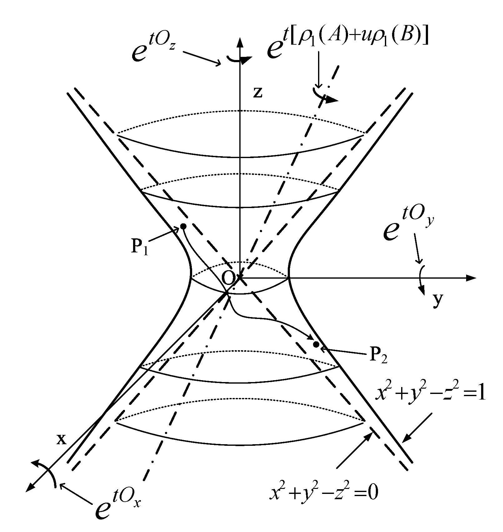
Figure 1: The topology of $SO(2,1)$.

V Examples

Example 1: Consider the quantum system with its Hamiltonian expressed as Gerry and Vrscay (1989)

$$H(t)=\omega_{0}K_{z}+u(t)K_{x},$$ (46)

where $K_{x}$ and $K_{z}$ are operators as defined in (4). The quantum system

$$i\hbar\dot{\psi}(t)=H(t)\psi(t)$$ (47)

is then a quantum control system that preserves $SU(1,1)$ coherent states Gerry (1985). Consider the positive discrete series unitary irreducible representations of $su(1,1)$ denoted by $\mathscr{D}^{+}(k)$, where $k$ is the so-called Bargmann index. The basis states $|m,k\rangle$ diagonalize the generator $K_{z}$ and the Casimir operator $C=K_{z}^{2}-K_{x}^{2}-K_{y}^{2}$ as follows: $K_{z}|m,k\rangle=(m+k)|m,k\rangle~{}(m=0,1,2,\cdots)$, and $C|m,k\rangle=k(k-1)|m,k\rangle$ with $k>0$. Then the operators $K_{\pm}=K_{x}{\pm}iK_{y}$ will act as raising and lowering operators,

$$\begin{array}[]{l}K_{+}|m,k\rangle=[(m+1)(m+2k)]^{1/2}|m+1,k\rangle,\\ K_{-}|m,k\rangle=[m(m+2k-1)]^{1/2}|m-1,k\rangle.\\ \end{array}$$ (48)

With the representation introduced above, the operators $K_{\pm}$ and $K_{z}$ are then identified as

$$K_{+}=\left(\begin{array}[]{ccccc}0&\sqrt{2k}&&&\\ &0&2\sqrt{2k+1}&&\\ &&0&3\sqrt{2k+2}&\\ &&&0&\ddots\\ &&&&\ddots\\ \end{array}\right),$$

$$K_{-}=\left(\begin{array}[]{ccccc}0&&&&\\ \sqrt{2k}&0&&&\\ &2\sqrt{2k+1}&0&&\\ &&3\sqrt{2k+2}&0&\\ &&&\ddots&\ddots\\ \end{array}\right),$$

$$K_{z}=\left(\begin{array}[]{ccccc}k+1&&&&\\ &k+2&&&\\ &&k+3&&\\ &&&k+4&\\ &&&&\ddots\\ \end{array}\right).$$

Following Perelomov Perelomov (1986), the $SU(1,1)$ coherent states are expressed as a linear combination of the basis vectors $|m,k\rangle~{}(m=0,1,2,\cdots)$, and can be obtained from the state $|0,k\rangle$ by the action of $\exp(\alpha{K_{+}}-\alpha^{*}{K_{-}})=\exp\{-2[\text{Im}(\alpha)(-iK_{x})+\text{Re}(\alpha)(-iK_{y})]\}$, where $\alpha$ is a complex number. Since, according to Theorem III.7, the equivalent system of the system (47)

$$\dot{X}(t)=[\omega_{0}\bar{K}_{z}+u(t)\bar{K}_{x}]X(t)$$ (49)

is controllable on $SU(1,1)$, it can be concluded that the transition between two arbitrary $SU(1,1)$ coherent states can be realized by controlling the quantum system (47).

Example 2: Consider the following control system evolving on $SO(2,1)$ Jurdjevic (1997)

$$\dot{Y}(t)=[O_{x}+u(t)O_{z}]Y(t),~{}Y(0)=I_{3},$$ (50)

and assume that the control $u(t)$ is restricted by $|u(t)|{\leq}C$, then the system is controllable if and only if $C>1$.

The associated system, evolving on $SU(1,1)$, is as follows

$$\dot{X}(t)=[\bar{K}_{x}+u(t)\bar{K}_{z}]X(t),~{}X(0)=I_{2}.$$ (51)

It can be verified that the set $\bar{\Omega}=\left\{-C{\leq}u{\leq}C|\left<\bar{K}_{x}+u\bar{K}_{z},\bar{K}_{x}^{\dagger}+u\bar{K}_{z}^{\dagger}\right>\right\}$ is nonempty if and only if $C>1$. Thus, according to the results obtained in Section III, system (51) is controllable when $C>1$.

Now we show that system (51) is uncontrollable when $C{\leq}1$. Write the solution of the evolution equation (51) as

$$X:=\left(\begin{array}[]{cc}x_{1}+ix_{2}&x_{3}-ix_{4}\\ x_{3}+ix_{4}&x_{1}-ix_{2}\end{array}\right),$$ (52)

then, with a few calculations, we have

$$\begin{split}\frac{d}{dt}[(x_{1}-x_{4})^{2}-(x_{2}-x_{3})^{2}]&=2u(x_{1}-x_{4})(x_{2}-x_{3})-[(x_{1}-x_{4})^{2}+(x_{2}-x_{3})^{2}]\\ &=-(1-u^{2})(x_{1}-x_{4})^{2}-[u(x_{1}-x_{4})-(x_{2}-x_{3})]^{2}\\ &\leq 0.\end{split}$$ (53)

This means that the function $[x_{1}(t)-x_{4}(t)]^{2}-[x_{2}(t)-x_{3}(t)]^{2}$ is nonincreasing for every trajectory of system (51) if $|u|{\leq}1$. Thus, the reachable set of system (51) never equals $SU(1,1)$, and the system is accordingly uncontrollable. As a result, system (50) is controllable if and only if $C>1$.

VI Conclusion

In this paper, we have studied the controllability properties of the quantum system evolving on the noncompact Lie group $SU(1,1)$. The criteria established in this article can be used to examine, for example, the ability to control the transitions between different $SU(1,1)$ coherent states. The results obtained in this paper also can be extended to the systems evolving on $SO(2,1)$ and $SL(2,\mathbb{R})$, because they are both homomorphic to $SU(1,1)$.

Appendix

In this appendix, we show that any hyperbolic $B$ can be converted into $\sqrt{\left<B,B^{\dagger}\right>}\bar{K}_{y}$ through a matrix $P{\in}SU(1,1)$, i.e., $PBP^{-1}=\sqrt{\left<B,B^{\dagger}\right>}\bar{K}_{y}$. Since $B$ is hyperbolic, we can expand it in the basis given in (6) as $B=x\bar{K}_{x}+y\bar{K}_{y}+z\bar{K}_{z}$, where $\left<B,B^{\dagger}\right>=x^{2}+y^{2}-z^{2}>0$.

First, one can find a matrix $P_{1}=e^{\alpha\bar{K}_{z}}{\in}SU(1,1)$, which satisfy

$$P_{1}BP_{1}^{-1}=\sqrt{x^{2}+y^{2}}\bar{K}_{y}+z\bar{K}_{z}.$$ (54)

Let $\alpha$ be the angle satisfying

$$\sin\alpha=\frac{x}{\sqrt{x^{2}+y^{2}}},~{}~{}\cos\alpha=\frac{y}{\sqrt{x^{2}+y^{2}}}.$$ (55)

According to the Baker-Hausdorff-Campbell formula

$$e^{M}Ne^{-M}=N+[M,N]+\frac{1}{2!}[M,[M,N]]+\frac{1}{3!}[M,[M,[M,N]]]+\cdots,$$ (56)

one can immediately obtain that

$$\begin{array}[]{l}e^{\alpha\bar{K}_{z}}Be^{-\alpha\bar{K}_{z}}=xe^{\alpha\bar{K}_{z}}\bar{K}_{x}e^{-\alpha\bar{K}_{z}}+ye^{\alpha\bar{K}_{z}}\bar{K}_{y}e^{-\alpha\bar{K}_{z}}+z\bar{K}_{z}\\ ~{}~{}~{}~{}~{}~{}~{}~{}~{}~{}=(x\cos\alpha-y\sin\alpha)\bar{K}_{x}+(x\sin\alpha+y\cos\alpha)\bar{K}_{y}+z\bar{K}_{z}\\ ~{}~{}~{}~{}~{}~{}~{}~{}~{}~{}=\sqrt{x^{2}+y^{2}}\bar{K}_{y}+z\bar{K}_{z}.\end{array}$$ (57)

Next, we show that there is a matrix $P_{2}=e^{\beta\bar{K}_{x}}$, in $SU(1,1)$, which can convert $\sqrt{x^{2}+y^{2}}\bar{K}_{y}+z\bar{K}_{z}$ into $\sqrt{\left<B,B^{\dagger}\right>}\bar{K}_{y}$. Since $x^{2}+y^{2}-z^{2}>0$, we can choose $\beta$ such that

$$\sinh\beta=\frac{z}{\sqrt{x^{2}+y^{2}-z^{2}}},~{}~{}\cosh\beta=\frac{\sqrt{x^{2}+y^{2}}}{\sqrt{x^{2}+y^{2}-z^{2}}}.$$ (58)

Make use of the formula given in (56) again, we have

$$\begin{array}[]{l}e^{\beta\bar{K}_{x}}(\sqrt{x^{2}+y^{2}}\bar{K}_{y}+z\bar{K}_{z})e^{-\beta\bar{K}_{x}}\\ ~{}~{}~{}=\sqrt{x^{2}+y^{2}}e^{\beta\bar{K}_{x}}\bar{K}_{y}e^{-\beta\bar{K}_{x}}+ze^{\beta\bar{K}_{x}}\bar{K}_{z}e^{-\beta\bar{K}_{x}}\\ ~{}~{}~{}=(\sqrt{x^{2}+y^{2}}\cosh\beta-z\sinh\beta)\bar{K}_{y}+(z\cosh\beta-\sqrt{x^{2}+y^{2}}\sinh\beta)\bar{K}_{z}\\ ~{}~{}~{}=\sqrt{x^{2}+y^{2}-z^{2}}\bar{K}_{y}\\ ~{}~{}~{}=\sqrt{\left<B,B^{\dagger}\right>}\bar{K}_{y}.\end{array}$$ (59)

Consequently, the $SU(1,1)$ matrix $e^{\beta\bar{K}_{x}}e^{\alpha\bar{K}_{z}}$ will convert $B$ into $\sqrt{\left<B,B^{\dagger}\right>}\bar{K}_{y}$ when it is hyperbolic.

References

• Sussmann (1972) H. J. Sussmann, J. Diff. Eqns. 12, 313 (1972).
• R.W.Brockket (1972) R.W.Brockket, SIAM J. Control 10, 265 (1972).
• Jurdjevic and Sussman (1972) V. Jurdjevic and H. J. Sussman, J. Diff. Eqns. 12, 313 (1972).
• Sussmann (1983) H. J. Sussmann, in Differential Geometric Control Theory, edited by R. W. Brockett, R. S. Millman, and H. J. Sussmann (Birkhauser, Boston, 1983), pp. 1–116.
• Huang et al. (1983) G. M. Huang, T. J. Tarn, and J. W. Clark, J. Math. Phys. 24, 2608 (1983).
• Ramakrishna et al. (1995) V. Ramakrishna, M. V. Salapaka, M. Dahleh, H. Rabitz, and A. Peirce, Phys. Rev. A 51, 960 (1995).
• Tarn et al. (2000) T. J. Tarn, J. W. Clark, and D. G. Lucarelli, in Proceedings of the 39th IEEE Conference on Decision and Control (Sydney, 2000), pp. 943–948.
• D’Alessandro (2000) D. D’Alessandro, Systems & Control Letters 41, 213 (2000).
• Schirmer et al. (2001) S. G. Schirmer, H. Fu, and A. I. Solomon, Phys. Rev. A 63, 063410 (2001).
• Lan et al. (2005) C. Lan, T.-J. Tarn, Q.-S. Chi, and J. Clark, J. Math. Phys. 46, 052102 (2005).
• Wu et al. (2006a) R.-B. Wu, T.-J. Tarn, and C. Li, Phys. Rev. A 73, 012719 (2006a).
• Puri (2001) R. R. Puri, Mathematical methods of quantum optics (Springer, 2001).
• Gerry and Vrscay (1989) C. C. Gerry and E. R. Vrscay, Phys. Rev. A 39, 5717 (1989).
• Gortel and Turski (1991) Z. W. Gortel and L. A. Turski, Phys. Rev. A 43, 3221 (1991).
• Bose (1985) S. K. Bose, J. Phys. A 18, 903 (1985).
• Agarwal and Banerji (2001) G. S. Agarwal and J. Banerji, Phys. Rev. A 64, 023815 (2001).
• Wu et al. (2006b) J.-W. Wu, C.-W. Li, R.-B. Wu, T.-J. Tarn, and J. Zhang, J. Phys. A 39, 13531 (2006b).
• Gerry (1985) C. C. Gerry, Phys. Rev. A 31, 2721 (1985).
• Walls (1983) D. F. Walls, Nature 306, 141 (1983).
• Vilenkin and Klimyk (1991) N. Vilenkin and A. U. Klimyk, Representation of Lie Groups and Special Functions, vol. Volume.1: Simplest Lie groups, special functions and integral transforms (Kluwer Academic Publishers, Boston, 1991).
• Ramakrishna et al. (2000) V. Ramakrishna, K. L. Flores, H. Rabitz, and R. J. Ober, Phys. Rev. A 62, 053409 (2000).
• Perelomov (1986) P. Perelomov, Generalized Coherent States and Their Applications (Springer-Verlag, Berlin, 1986).
• Jurdjevic (1997) V. Jurdjevic, Geometric Control Theory (Cambridge University Press, 1997).