Baryon vector and axial content up to the $7Q$ component

We have used the light-cone formulation of Chiral-Quark Soliton Model to investigate the vector and axial content of octet, decuplet and hypothetical antidecuplet in the flavor $SU(3)$ symmetry limit. We have extended previous works by computing the $7Q$ contribution to vector and axial charges for the octet and antidecuplet but stayed at the $5Q$ sector for the decuplet where the full computation needs much more time. As expected the $7Q$ component has a weaker impact on the quantities but still changes them by a few percent. We give also a detailed decomposition of those charges into flavor, valence quark, sea quark and antiquark contributions. Many of them are of course not (yet) measured or estimated and constitute then a theoretical estimation. Among the different interesting observations made in this work are the explicit quadrupole deformation of decuplet baryons due to the pion field and the sum of quark spins larger than the pentaquark one.

1 Introduction

Chiral-Quark Soliton Model ($\chi$QSM) has recently been formulated on the light cone or, equivalently, in the Infinite Momentum Frame (IMF) [1, 2]. This provides a new approach for extracting predictions out of the model. The light-cone formulation is attractive in many ways. For example, light-cone wave functions are particularly well suited to compute matrix elements of operators. One can even choose to work in a specific frame where the annoying part of currents, i.e. pair creation and annihilation part, does not contribute. On the top of that it is in principle also easy to compute parton distributions once light-cone wave functions are known.

The technique has already been used to study vector and axial charges of the nucleon and $\Theta^{+}$ pentaquark width up to the $5Q$ component without [2] and with [3] quark orbital angular momentum. In this approach it has been shown that relativistic corrections (quark angular momentum and sea-quark pairs) reduce the naive quark model value $\frac{5}{3}$ for the nucleon axial charge $g^{(3)}_{A}$ down to a value close to $1.257$ observed in beta decays.

The baryon structure is of capital importance for our understanding of QCD. In this non-perturbative regime the theory cannot be solved and models are needed to understand the physics at this scale. While a picture of the baryon as a system of 3 nonrelativistic quarks seems to explain rather well magnetic moments, masses and meson-baryon couplings, one observes that in polarized Deep Inelastic Scattering (DIS) processes there are other ingredients. Let us mention for example the violation of Ellis-Jaffe sum rule revealing the presence of hidden flavor in the nucleon. It has also been observed that the quarks contribute only to $\sim 30\%$ of the total nucleon spin leading to what is called the “spin crisis”. It is clear that the missing angular momentum can be attributed to quark orbital momentum and gluon angular momentum. Unfortunately, the individual contributions are not known. Many models try to improve the so-called Naive Quark Model (NQM) by taking into account other degrees of freedom and/or general features of QCD such as special relativity and approximate chiral symmetry.

$\chi$QSM is a model based on chiral symmetry. A baryon is considered as made of $N_{C}$ valence quarks living in a relativistic mean chiral field. This mean field is a soliton with maximal symmetry, namely a hedgehog pion field. A specific baryon then corresponds to a specific rotational excitation of the solitonic field. This model can be considered as some interpolation between two a priori orthogonal pictures: Constituent Quark Model where baryons are made of valence quarks exclusively and Skyrme Model where baryons are solitons of the pion field. $\chi$QSM has both degrees of freedom. Here baryons are indeed made of valence quarks but living in a solitonic relativistic mean chiral field. In the limit where the pion field is weak, the Dirac sea is weakly distorted and thus carry small energy $E_{\textrm{sea}}\simeq 0$. The valence level is shallow $E_{\textrm{lev}}\simeq M_{Q}$ and hence the valence quarks are nonrelativistic. This is very similar to the Constituent Quark Model picture. In the limit where the pion field is large, the bound-state level is so deep that it joins the Dirac sea. The whole nucleon mass is given by $E_{\textrm{sea}}$ which can be expanded in derivatives of the mean field, the first terms being close to the Skyrme Model Lagrangian.

This model has been mostly studied in the so-called “instant form”, i.e. with the usual parametrization of space-time $x=(t,\mathbf{x})$ and reproduced successfully many experimental results [4, 5]. In the instant form, the sea can be treated as a whole but a slowly rotating soliton approximation has to be invoked. Although this approximation is well justified for ordinary baryons (octet and decuplet) it is questionable for the exotic ones (antidecuplet) [2]. The light-cone approach to $\chi$QSM is complementary. Here we cannot treat the whole Dirac sea at once. One has to perform an expansion of the baryon wave function in Fock space. On the other hand, we can compute exact rotations without referring to the large-$N_{C}$ limit for their evaluation. Hence, there is a priori no direct connection between the moment of inertia of the soliton and the overlap of individual quark wave function. Moreover, studying models on the light cone is always very interesting since the description is closer to experimental situation where baryons are usually moving with high velocity.

In the IMF formulation of $\chi$QSM, it has been possible to write a general expression for baryon light-cone wave functions. By computing matrix elements of operators, one can access the flavor and spin content of the baryons and work explicitly with $0,1,2,\ldots,n$ additional quark-antiquark pairs in a fully relativistic way. On the top of that the solitonic approach allows one to treat all light baryons in a simple and unique elegant way. Since the $5Q$ component is important to understand the nucleon structure one should by analogy care about the $7Q$ component in pentaquark. On the top of that it is also an a posteriori check that the expansion in the number of quark-antiquark pairs is justified.

This paper is organized as follows. In section 2 we present in a short way the model formulated in the IMF and give the explicit definitions of the quantities used. Then we indicate how to compute the charges by means of matrix elements in each Fock sector in section 3. After contraction over all color, spin, isospin and flavor indices one is left with scalar overlap integrals. Physical quantities are then just specific linear combinations of those scalar overlap integrals determined by $SU(3)$ symmetry. The explicit expressions of those integrals are presented in section 4. Since our approach is restricted to flavor $SU(3)$ symmetry we give tables making it explicit and present the parametrization used in section 5. Our results can be found in section 6. First we give the formal combinations and then the numerical evaluation, followed by a discussion and comparison with experimental knowledge.

2 $\chi$QSM on the Light Cone

Chiral-Quark Soliton Model ($\chi$QSM) is a model proposed to mimic low-energy QCD. It emphasizes the role of constituent quarks of mass $M$ and pseudoscalar mesons as the relevant degrees of freedom and is based on the following effective Lagrangian

$$\mathcal{L}_{\chi QSM}=\bar{\psi}(p)(p\!\!\!/-MU^{\gamma_{5}})\psi(p),$$ (1)

where $U^{\gamma_{5}}$ is a (flavor) $SU(3)$ matrix. We used the $SU(2)$ hedgehog Ansatz for the soliton field trivially embedded in $SU(3)$

$$U^{\gamma_{5}}=\left(\begin{array}[]{cc}U_{0}&0\\ 0&1\end{array}\right),\qquad U_{0}=e^{in^{a}\tau^{a}P(r)\gamma_{5}}$$ (2)

with $\tau^{a}$ the usual $SU(2)$ Pauli matrices and $n^{a}=r^{a}/r$ the unit vector pointing in the direction of $\mathbf{r}$. Note that the hedgehog Ansatz implies that a rotation in ordinary space ($n^{a}$) can be compensated by a rotation in isospin space ($\tau^{a}$). The profile function $P(r)$ is determined by topological constraints and minimization of the energy of the system.

Within this model it has been shown [1, 2] that one can write a general expression for $SU(3)$ baryon wave functions

$$|\Psi_{B}\rangle=\left[\prod_{\textrm{color}=1}^{N_{C}}\int(\mathrm{d}\mathbf{p})\,F(\mathbf{p})\,a^{\dagger}(\mathbf{p})\right]\exp\left(\int(\mathrm{d}\mathbf{p})(\mathrm{d}\mathbf{p}^{\prime})\,a^{\dagger}(\mathbf{p})\,W(\mathbf{p},\mathbf{p}^{\prime})\,b^{\dagger}(\mathbf{p}^{\prime})\right)|\Omega_{0}\rangle.$$ (3)

This expression may look somewhat complicated at first view but is in fact really transparent. The model describes baryons as $N_{C}$ quarks populating the valence level with wave function $F$ accompanied by a whole sea of quark-antiquark pairs represented by the coherent exponential. The wave function of such a quark-antiquark pair is $W$. For a specific baryon, one has to rotate each quark by a $SU(3)$-matrix $R$ and each antiquark by $R^{\dagger}$ and project the whole wave function on the quantum number of the specific baryon $\int\mathrm{d}R\,B_{k}^{*}(R)$, where $B_{k}^{*}(R)$ represents the way the baryon is transformed by $SU(3)$. The full expression [2] for the light-cone baryon wave function contains color $\alpha$, flavor $f$, isospin $j$ and spin $\sigma$ indices

$$\begin{split}|\Psi_{k}(B)\rangle&=\int\mathrm{d}R\,B_{k}^{*}(R)\,\epsilon^{\alpha_{1}\alpha_{2}\alpha_{3}}\left[\prod_{n=1}^{3}\int(\mathrm{d}\mathbf{p}_{n})\,R_{j_{n}}^{f_{n}}\,F^{j_{n}\sigma_{n}}(\mathbf{p}_{n})\,a^{\dagger}_{\alpha_{n}f_{n}\sigma_{n}}(\mathbf{p}_{n})\right]\\ &\times\quad\exp\left(\int(\mathrm{d}\mathbf{p})(\mathrm{d}\mathbf{p}^{\prime})\,\delta_{\alpha^{\prime}}^{\alpha}\,a^{\dagger}_{\alpha f\sigma}(\mathbf{p})\,R^{f}_{j}\,W^{j\sigma}_{j^{\prime}\sigma^{\prime}}(\mathbf{p},\mathbf{p}^{\prime})\,R^{{\dagger}j^{\prime}}_{f^{\prime}}\,b^{{\dagger}\alpha^{\prime}f^{\prime}\sigma^{\prime}}(\mathbf{p}^{\prime})\right)|\Omega_{0}\rangle,\end{split}$$ (4)

where we have considered the physical case $N_{C}=3$. The three valence quarks are always antisymmetric in color $\epsilon^{\alpha_{1}\alpha_{2}\alpha_{3}}$ and the additional quark-antiquark pairs are color singlets $\delta_{\alpha^{\prime}}^{\alpha}$. This wave function is supposed provide a lot of information about all light baryons.

2.1 Valence wave function

On the light cone the valence level wave function $F$ is given by

$$F^{j\sigma}_{\textrm{lev}}(z,\mathbf{p}_{\perp})=\sqrt{\frac{\mathcal{M}}{2\pi}}\left[\epsilon^{j\sigma}h(p)+(p_{z}\mathds{1}+i\mathbf{p}_{\perp}\times\tau_{\perp})^{\sigma}_{\sigma^{\prime}}\epsilon^{j\sigma^{\prime}}\frac{j(p)}{|\mathbf{p}|}\right]_{p_{z}=z\mathcal{M}-E_{\textrm{lev}}}$$ (5)

where $j$ and $\sigma$ are isospin and spin indices respectively, $z$ is the fraction of baryon longitudinal momentum carried by the quark, $\mathbf{p}_{\perp}$ is its transverse momentum and $\mathcal{M}$ is the classical soliton mass. The functions $h(p)$ and $j(p)$ are Fourier transforms of the upper ($L=0$) $h(r)$ and lower ($L=1$) $j(r)$ components of the spinor solution (see Fig.2) of the static Dirac equation in the mean field with eigenenergy $E_{\textrm{lev}}$

$$\psi_{\textrm{lev}}(\mathbf{x})=\left(\begin{array}[]{c}\epsilon^{ji}h(r)\\ -i\epsilon^{jk}(\mathbf{n}\cdot\sigma)^{i}_{k}\,j(r)\end{array}\right),\qquad\left\{\begin{array}[]{c}h^{\prime}+h\,M\sin P-j(M\cos P+E_{\textrm{lev}})=0\\ j^{\prime}+2j/r-j\,M\sin P-h(M\cos P-E_{\textrm{lev}})=0\end{array}\right.,$$ (6)

where $P(r)$, the profile function of the soliton, is fairly approximated by [6, 7] (see Fig.2)

$$P(r)=2\arctan\left(\frac{r_{0}^{2}}{r^{2}}\right),\qquad r_{0}\approx\frac{0.8}{M}.$$ (7)

Figure 1: Upper $s$-wave component $h(r)$ (solid) and lower $p$-wave component $j(r)$ (dashed) of the bound-state quark level in light baryons. Each of the three valence quarks has energy $E_{\textrm{lev}}=200$ MeV. Horizontal axis has units of $1/M=0.57$ fm.

Figure 2: Profile of the self-consistent chiral field $P(r)$ in light baryons. The horizontal axis unit is $r_{0}=0.8/M=0.46$ fm.

2.2 Pair wave function

The quark-antiquark pair wave function $W$ can be written in terms of the Fourier transform of the chiral field with chiral circle condition $\Pi^{2}+\Sigma^{2}=1$, $U_{0}=\Sigma+i\Pi\gamma_{5}$. The chiral field is then given by

$$\Pi=\mathbf{n}\cdot\tau\sin P(r),\qquad\Sigma(r)=\cos P(r)$$ (8)

and its Fourier transform by

$$\Pi(\mathbf{q})^{j}_{j^{\prime}}=\int\mathrm{d}^{3}\mathbf{x}\,e^{-i\mathbf{q}\cdot\mathbf{x}}(\mathbf{n}\cdot\tau)^{j}_{j^{\prime}}\sin P(r),\qquad\Sigma(\mathbf{q})^{j}_{j^{\prime}}=\int\mathrm{d}^{3}\mathbf{x}\,e^{-i\mathbf{q}\cdot\mathbf{x}}(\cos P(r)-1)\delta^{j}_{j^{\prime}},$$ (9)

where $j$ and $j^{\prime}$ are the isospin indices of the quark and antiquark, respectively. The pair wave function is obtained by considering the expansion of the quark propagator [1] in the mean field in terms of the chiral interaction $V=U_{0}-1$. After the boost to the IMF, the pair wave function appears as a function of the fractions of the baryon longitudinal momentum carried by the quark $z$ and antiquark $z^{\prime}$ of the pair and their transverse momenta $\mathbf{p}_{\perp}$, $\mathbf{p}^{\prime}_{\perp}$

$$W^{j\sigma}_{j^{\prime}\sigma^{\prime}}(z,\mathbf{p}_{\perp};z^{\prime},\mathbf{p}^{\prime}_{\perp})=\frac{M\mathcal{M}}{2\pi Z}\left\{\Sigma^{j}_{j^{\prime}}(\mathbf{q})[M(z^{\prime}-z)\tau_{3}+\mathbf{Q}_{\perp}\cdot\tau_{\perp}]^{\sigma}_{\sigma^{\prime}}+i\Pi^{j}_{j^{\prime}}(\mathbf{q})[-M(z^{\prime}+z)\mathds{1}+i\mathbf{Q}_{\perp}\times\tau_{\perp}]^{\sigma}_{\sigma^{\prime}}\right\},$$ (10)

where $\mathbf{q}=((\mathbf{p}+\mathbf{p}^{\prime})_{\perp},(z+z^{\prime})\mathcal{M})$ is the three-momentum of the pair as a whole transferred from the background fields $\Sigma(\mathbf{q})$ and $\Pi(\mathbf{q})$. As earlier $j$ and $j^{\prime}$ are isospin and $\sigma$ and $\sigma^{\prime}$ are spin indices with the prime for the antiquark. In order to condense the notations we used

$$Z=\mathcal{M}^{2}zz^{\prime}(z+z^{\prime})+z(p^{\prime 2}_{\perp}+M^{2})+z^{\prime}(p^{2}_{\perp}+M^{2}),\qquad\mathbf{Q}_{\perp}=z\mathbf{p}^{\prime}_{\perp}-z^{\prime}\mathbf{p}_{\perp}.$$ (11)

A more compact form for this wave function can be obtained by means of the following two variables

$$y=\frac{z^{\prime}}{z+z^{\prime}},\qquad\mathcal{Q}_{\perp}=\frac{z\mathbf{p}^{\prime}_{\perp}-z^{\prime}\mathbf{p}_{\perp}}{z+z^{\prime}}.$$ (12)

The pair wave function then takes the form

$$W^{j\sigma}_{j^{\prime}\sigma^{\prime}}(y,\mathbf{q},\mathcal{Q}_{\perp})=\frac{M\mathcal{M}}{2\pi}\,\frac{\Sigma^{j}_{j^{\prime}}(\mathbf{q})[M(2y-1)\tau_{3}+\mathcal{Q}_{\perp}\cdot\tau_{\perp}]^{\sigma}_{\sigma^{\prime}}+i\Pi^{j}_{j^{\prime}}(\mathbf{q})[-M\mathds{1}+i\mathcal{Q}_{\perp}\times\tau_{\perp}]^{\sigma}_{\sigma^{\prime}}}{\mathcal{Q}^{2}_{\perp}+M^{2}+y(1-y)\mathbf{q}^{2}}.$$ (13)

2.3 Rotational wave function

To obtain the wave function of a specific baryon with given spin projection $k$, one has to rotate the soliton in ordinary and flavor spaces and then project on quantum numbers of this specific baryon. For example, one has to compute the following integral to obtain the neutron rotational wave function in the $3Q$ sector

$$T(n^{0})_{k,j_{1}j_{2}j_{3}}^{f_{1}f_{2}f_{3}}=\int\mathrm{d}R\,n_{k}(R)^{*}R^{f_{1}}_{j_{1}}R^{f_{2}}_{j_{2}}R^{f_{3}}_{j_{3}},$$ (14)

where $R$ is a $SU(3)$ matrix and $n_{k}(R)^{*}=\frac{\sqrt{8}}{24}\,\epsilon_{kl}R^{{\dagger}l}_{2}R^{3}_{3}$ represents the way that the neutron is transformed under $SU(3)$ rotations. This integral means that the neutron state $n_{k}(R)^{*}$ is projected onto the $3Q$ sector $R^{f_{1}}_{j_{1}}R^{f_{2}}_{j_{2}}R^{f_{3}}_{j_{3}}$ by means of the integration over all $SU(3)$ matrices $\int\mathrm{d}R$. By contracting this rotational wave function $T(n^{0})_{k,j_{1}j_{2}j_{3}}^{f_{1}f_{2}f_{3}}$ with the nonrelativistic $3Q$ wave function $\epsilon^{j_{1}\sigma_{1}}\epsilon^{j_{2}\sigma_{2}}\epsilon^{j_{3}\sigma_{3}}h(p_{1})h(p_{2})h(p_{3})$ one finally obtains the nonrelativistic neutron wave function

$$|n^{0}\rangle_{k}^{f_{1}f_{2}f_{3},\sigma_{1}\sigma_{2}\sigma_{3}}=\frac{\sqrt{8}}{24}\,\epsilon^{f_{1}f_{2}}\epsilon^{\sigma_{1}\sigma_{2}}\delta^{f_{3}}_{2}\delta^{\sigma_{3}}_{k}h(p_{1})h(p_{2})h(p_{3})+\textrm{cyclic permutations of 1,2,3.}$$ (15)

This expression means that there is a $ud$ pair in spin-isospin zero combination $\epsilon^{f_{1}f_{2}}\epsilon^{\sigma_{1}\sigma_{2}}$ and that the third quark is a down quark $\delta^{f_{3}}_{2}$ and carries the whole spin of the neutron $\delta^{\sigma_{3}}_{k}$. This is in fact exactly the $SU(6)$ spin-flavor wave function for the neutron.

The rotational wave function of octet, decuplet and antidecuplet in the $3Q$, $5Q$ and $7Q$ sectors can all be found in the Appendix of this paper.

3 Currents, charges and matrix elements

A typical physical observable is the matrix element of some operator (preferably written in terms of quark annihilation-creation operators $a$, $b$, $a^{\dagger}$, $b^{\dagger}$) sandwiched between the initial and final baryon wave functions. These wave functions are superpositions of Fock states obtained by expanding the coherent exponential in eq. (3). One can reasonably expect that the Fock states with the lowest number of quarks will give the main contribution. If one uses the Drell frame $q^{+}=0$ [8, 9] where $q$ is the total momentum transfer, then the vector $\bar{\psi}\gamma^{+}\psi$ and axial $\bar{\psi}\gamma^{+}\gamma^{5}\psi$ currents can neither create nor annihilate any quark-antiquark pair. This is a big advantage of the light-cone formulation since one needs to compute diagonal transitions only, i.e. $3Q$ into $3Q$, $5Q$ into $5Q$, $\ldots$ and not $3Q$ into $5Q$ for example.

In the $3Q$ sector, since all (valence) quarks are on the same footing, all the possible contractions of creation-annihilation operators are equivalent. One can use a diagram to represent these contractions. The contractions without any current operator acting on a quark line correspond to the normalization of the state. We choose the simplest one where all quarks with the same label are connected, see Fig.4.

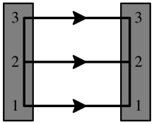
Figure 3: Schematic representation of the $3Q$ normalization. Each quark line stands for the color, flavor and spin contractions $\delta^{\alpha_{i}}_{\alpha^{\prime}_{i}}\delta^{f_{i}}_{f^{\prime}_{i}}\delta^{\sigma_{i}}_{\sigma^{\prime}_{i}}\int\mathrm{d}z^{\prime}_{i}\,\mathrm{d}^{2}\mathbf{p}^{\prime}_{i\perp}\delta(z_{i}-z^{\prime}_{i})$ $\delta^{(2)}(\mathbf{p}_{i\perp}-\mathbf{p}^{\prime}_{i\perp})$. The large dark rectangles stand for the three initial (left) and final (right) valence quarks antisymmetrized in color $\epsilon_{\alpha_{1}\alpha_{2}\alpha_{3}}$.

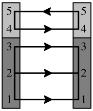
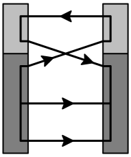
Figure 4: Schematic representation of the $5Q$ direct (left) and exchange (right) contributions to the normalization. The quark-antiquark pairs are represented by small light rectangles and are in color singlet $\delta^{\alpha_{4}}_{\alpha_{5}}$.

In the $5Q$ sector, all contractions are equivalent to either the so-called “direct” diagram or the “exchange” diagram, see Fig.4. In the direct diagram, all quarks with the same label are connected while in the exchange one, a valence quark is exchanged with the quark of the sea pair. It has appeared in a previous work [3] that exchange diagrams do not contribute much and can thus be neglected (there is no disconnected quark loop). So we use only the direct contributions throughout this paper.

In the $7Q$ sector there are 5 types of diagrams, see Fig.5. The three last diagrams involve at least an exchange of a valence quark with a sea quark. Those are neglected in the present work by analogy with the $5Q$ sector. In the second and fourth diagrams the two pairs exchange their quark (or antiquark) and are likely negligible. We therefore expect that the first diagram gives the major contribution in the $7Q$ sector. A mathematical argument is that contraction over color indices favors this diagram by at least a factor 3 (there is at least one more disconnected quark loop compared to the other diagrams). A physical argument would be that this diagram represents a process where nothing really happens and is thus expected to be dominant compared to the other diagrams where quarks exchange their roles.

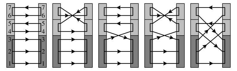
Figure 5: Schematic representation of the $7Q$ contributions to the normalization.

The vector and axial operators act on each quark line. In the present approach it is easy to compute separately the contributions coming from the valence quarks, the sea quarks and antiquarks, see Fig.6.

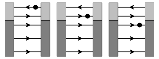
Figure 6: Schematic representation of the three types of $5Q$ contributions to the charges: antiquark (left), sea quark (center) and valence quark (right) contributions.

These diagrams represent some contraction of color, spin, isospin and flavor indices. For example, the sum of the three diagrams in the $5Q$ sector with the vector current acting on the quark lines represents the following expression

$$\begin{split}V^{(5)}(1\to 2)&=\frac{108}{2}\,\delta^{k}_{l}\,T(1)^{f_{1}f_{2}f_{3}f_{4},j_{5}}_{j_{1}j_{2}j_{3}j_{4},f_{5},k}\,T(2)_{f_{1}f_{2}g_{3}g_{4},l_{5}}^{l_{1}l_{2}l_{3}l_{4},g_{5},l}\int(\mathrm{d}p_{1-5})\\ &\times F^{j_{1}\sigma_{1}}(p_{1})F^{j_{2}\sigma_{2}}(p_{2})F^{j_{3}\sigma_{3}}(p_{3})W^{j_{4}\sigma_{4}}_{j_{5}\sigma_{5}}(p_{4},p_{5})F^{\dagger}_{l_{1}\sigma_{1}}(p_{1})F^{\dagger}_{l_{2}\sigma_{2}}(p_{2})F^{\dagger}_{l_{3}\tau_{3}}(p_{3})W_{c\,l_{4}\tau_{4}}^{l_{5}\tau_{5}}(p_{4},p_{5})\\ &\times\left[-\delta^{g_{3}}_{f_{3}}\delta^{g_{4}}_{f_{4}}\boldsymbol{J^{f_{5}}_{g_{5}}}\delta^{\tau_{3}}_{\sigma_{3}}\delta^{\tau_{4}}_{\sigma_{4}}\boldsymbol{\delta_{\tau_{5}}^{\sigma_{5}}}+\delta^{g_{3}}_{f_{3}}\boldsymbol{J^{g_{4}}_{f_{4}}}\delta^{f_{5}}_{g_{5}}\delta^{\tau_{3}}_{\sigma_{3}}\boldsymbol{\delta^{\tau_{4}}_{\sigma_{4}}}\delta_{\tau_{5}}^{\sigma_{5}}+3\boldsymbol{J^{g_{3}}_{f_{3}}}\delta^{g_{4}}_{f_{4}}\delta^{f_{5}}_{g_{5}}\boldsymbol{\delta^{\tau_{3}}_{\sigma_{3}}}\delta^{\tau_{4}}_{\sigma_{4}}\delta_{\tau_{5}}^{\sigma_{5}}\right],\end{split}$$ (16)

where $J^{f}_{g}$ is the flavor content of the current. The axial charge is easily obtained from the vector one. One just has to replace the averaging over baryon spin by $\frac{1}{2}(-\sigma_{3})^{k}_{l}$ and the axial charge operator involves now $\boldsymbol{(-\sigma_{3})^{\tau_{i}}_{\sigma_{i}}}$ instead of $\boldsymbol{\delta^{\tau_{i}}_{\sigma_{i}}}$. One then has

$$\begin{split}A^{(5)}(1\to 2)&=\frac{108}{2}\,(-\sigma_{3})^{k}_{l}\,T(1)^{f_{1}f_{2}f_{3}f_{4},j_{5}}_{j_{1}j_{2}j_{3}j_{4},f_{5},k}\,T(2)_{f_{1}f_{2}g_{3}g_{4},l_{5}}^{l_{1}l_{2}l_{3}l_{4},g_{5},l}\int(\mathrm{d}p_{1-5})\\ &\times F^{j_{1}\sigma_{1}}(p_{1})F^{j_{2}\sigma_{2}}(p_{2})F^{j_{3}\sigma_{3}}(p_{3})W^{j_{4}\sigma_{4}}_{j_{5}\sigma_{5}}(p_{4},p_{5})F^{\dagger}_{l_{1}\sigma_{1}}(p_{1})F^{\dagger}_{l_{2}\sigma_{2}}(p_{2})F^{\dagger}_{l_{3}\tau_{3}}(p_{3})W_{c\,l_{4}\tau_{4}}^{l_{5}\tau_{5}}(p_{4},p_{5})\\ &\times\left[-\delta^{g_{3}}_{f_{3}}\delta^{g_{4}}_{f_{4}}\boldsymbol{J^{f_{5}}_{g_{5}}}\delta^{\tau_{3}}_{\sigma_{3}}\delta^{\tau_{4}}_{\sigma_{4}}\boldsymbol{(-\sigma_{3})_{\tau_{5}}^{\sigma_{5}}}+\delta^{g_{3}}_{f_{3}}\boldsymbol{J^{g_{4}}_{f_{4}}}\delta^{f_{5}}_{g_{5}}\delta^{\tau_{3}}_{\sigma_{3}}\boldsymbol{(-\sigma_{3})^{\tau_{4}}_{\sigma_{4}}}\delta_{\tau_{5}}^{\sigma_{5}}+3\boldsymbol{J^{g_{3}}_{f_{3}}}\delta^{g_{4}}_{f_{4}}\delta^{f_{5}}_{g_{5}}\boldsymbol{(-\sigma_{3})^{\tau_{3}}_{\sigma_{3}}}\delta^{\tau_{4}}_{\sigma_{4}}\delta_{\tau_{5}}^{\sigma_{5}}\right].\end{split}$$ (17)

4 Scalar overlap integrals

The contractions in previous section are easily performed by Mathematica over all flavor $(f,g)$, isospin $(j,l)$ and spin $(\sigma,\tau)$ indices. One is then left with scalar integrals over longitudinal $z$ and transverse $\mathbf{p}_{\perp}$ momenta of the quarks. The integrals over relative transverse momenta in the quark-antiquark pair are generally UV divergent. We have chosen to use the Pauli-Villars regularization with mass $M_{\textrm{PV}}=556.8$ MeV (this value being chosen from the requirement that the pion decay constant $F_{\pi}=93$ MeV is reproduced for $M=345$ MeV).

For convenience we introduce the probability distribution $\Phi^{I}(z,\mathbf{q}_{\perp})$ seen by a vector ($I=V$) or an axial ($I=A$) probe, that three valence quarks leave the longitudinal fraction $z=q_{z}/\mathcal{M}$ and the transverse momentum $\mathbf{q}_{\perp}$ to the quark-antiquark pair(s)

$$\Phi^{I}(z,\mathbf{q}_{\perp})=\int\mathrm{d}z_{1,2,3}\frac{\mathrm{d}^{2}\mathbf{p}_{1,2,3\perp}}{(2\pi)^{6}}\,\delta(z+z_{1}+z_{2}+z_{3}-1)(2\pi)^{2}\delta^{(2)}(\mathbf{q}_{\perp}+\mathbf{p}_{1\perp}+\mathbf{p}_{2\perp}+\mathbf{p}_{3\perp})D^{I}(p_{1},p_{2},p_{3}).$$ (18)

The function $D^{I}(p_{1},p_{2},p_{3})$ is given in terms of the upper and lower valence wave functions $h(p)$ and $j(p)$ as follows

$$\begin{split}D^{V}(p_{1},p_{2},p_{3})&=h^{2}_{1}h^{2}_{2}h^{2}_{3}+6h^{2}_{1}h^{2}_{2}\left[h_{3}\frac{p_{3z}}{|\mathbf{p}_{3}|}j_{3}\right]+3h^{2}_{1}h^{2}_{2}j^{2}_{3}+12h^{2}_{1}\left[h_{2}\frac{p_{2z}}{|\mathbf{p}_{2}|}j_{2}\right]\left[h_{3}\frac{p_{3z}}{|\mathbf{p}_{3}|}j_{3}\right]\\ &+12h^{2}_{1}\left[h_{2}\frac{p_{2z}}{|\mathbf{p}_{2}|}j_{2}\right]j^{2}_{3}+8\left[h_{1}\frac{p_{1z}}{|\mathbf{p}_{1}|}j_{1}\right]\left[h_{2}\frac{p_{2z}}{|\mathbf{p}_{2}|}j_{2}\right]\left[h_{3}\frac{p_{3z}}{|\mathbf{p}_{3}|}j_{3}\right]+3h^{2}_{1}j^{2}_{2}j^{2}_{3}\\ &+12\left[h_{1}\frac{p_{1z}}{|\mathbf{p}_{1}|}j_{1}\right]\left[h_{2}\frac{p_{2z}}{|\mathbf{p}_{2}|}j_{2}\right]j^{2}_{3}+6\left[h_{1}\frac{p_{1z}}{|\mathbf{p}_{1}|}j_{1}\right]j^{2}_{2}j^{2}_{3}+j^{2}_{1}j^{2}_{2}j^{2}_{3},\end{split}$$ (19)

$$\begin{split}D^{A}(p_{1},p_{2},p_{3})&=h^{2}_{1}h^{2}_{2}h^{2}_{3}+6h^{2}_{1}h^{2}_{2}\left[h_{3}\frac{p_{3z}}{|\mathbf{p}_{3}|}j_{3}\right]+h^{2}_{1}h^{2}_{2}\frac{2p_{3z}^{2}+p_{3}^{2}}{p_{3}^{2}}j^{2}_{3}+12h^{2}_{1}\left[h_{2}\frac{p_{2z}}{|\mathbf{p}_{2}|}j_{2}\right]\left[h_{3}\frac{p_{3z}}{|\mathbf{p}_{3}|}j_{3}\right]\\ &+4h^{2}_{1}\left[h_{2}\frac{p_{2z}}{|\mathbf{p}_{2}|}j_{2}\right]\frac{2p_{3z}^{2}+p_{3}^{2}}{p_{3}^{2}}j^{2}_{3}+8\left[h_{1}\frac{p_{1z}}{|\mathbf{p}_{1}|}j_{1}\right]\left[h_{2}\frac{p_{2z}}{|\mathbf{p}_{2}|}j_{2}\right]\left[h_{3}\frac{p_{3z}}{|\mathbf{p}_{3}|}j_{3}\right]+h^{2}_{1}j^{2}_{2}\frac{4p_{3z}^{2}-p_{3}^{2}}{p_{3}^{2}}j^{2}_{3}\\ &+4\left[h_{1}\frac{p_{1z}}{|\mathbf{p}_{1}|}j_{1}\right]\left[h_{2}\frac{p_{2z}}{|\mathbf{p}_{2}|}j_{2}\right]\frac{2p_{3z}^{2}+p_{3}^{2}}{p_{3}^{2}}j^{2}_{3}+2\left[h_{1}\frac{p_{1z}}{|\mathbf{p}_{1}|}j_{1}\right]j^{2}_{2}\frac{4p_{3z}^{2}-p_{3}^{2}}{p_{3}^{2}}j^{2}_{3}+j^{2}_{1}j^{2}_{2}\frac{2p_{3z}^{2}-p_{3}^{2}}{p_{3}^{2}}j^{2}_{3},\end{split}$$ (20)

where we have used $h_{i}\equiv h(p_{i})$ and $j_{i}\equiv j(p_{i})$.

In the nonrelativistic limit one has $j(p)=0$ and thus $D^{V}(p_{1},p_{2},p_{3})=D^{A}(p_{1},p_{2},p_{3})$ as it should be. Indeed, nonrelativistic quarks have no orbital angular momentum and then axial and vector probes see the same valence quark distribution. In other words, because of the absence of quark angular momentum, a quark with helicity $\pm$ has spin $z$-projection $\pm 1/2$, respectively.

4.1 $3Q$ scalar integrals

In the $3Q$ sector there is no quark-antiquark pair. There are then two integrals only, one for the vector case

$$\Phi^{V}(0,0)$$ (21)

and one for the axial one

$$\Phi^{A}(0,0),$$ (22)

where the null argument indicates that the whole baryon momentum is carried by the three valence quarks. Let us remind that in this sector, spin-flavor wave functions obtained by the projection technique are equivalent to those given by $SU(6)$ symmetry. One then naturally obtains the same results for the charges as those given by $SU(6)$ NQM, excepted that axial quantities are multiplied by the factor $\Phi^{A}(0,0)/\Phi^{V}(0,0)$. This is similar to the usual approach based on the Melosh rotation [10]. In usual light-cone models one starts with nonrelativistic $SU(6)$ wave functions and then performs a Melosh rotation on the spinors to obtain the helicity basis, particularly well suited for light-cone treatment. This rotation introduces orbital angular momentum somewhat artificially. The net effect of this rotation is the introduction of a Melosh factor to the observables compared with NQM predictions

$$q=M_{V}\,q_{NQM},\qquad\Delta q=M_{A}\,\Delta q_{NQM}.$$ (23)

We will discuss this point more intensively in a further work.

4.2 $5Q$ scalar integrals

In the $5Q$ sector there is one quark-antiquark pair and only seven integrals are needed. These integrals can be written in the general form

$$K^{I}_{J}=\frac{M^{2}}{2\pi}\int\frac{\mathrm{d}^{3}\mathbf{q}}{(2\pi)^{3}}\,\Phi^{I}\left(\frac{q_{z}}{\mathcal{M}},\mathbf{q}_{\perp}\right)\theta(q_{z})\,q_{z}\,G_{J}(q_{z},\mathbf{q}_{\perp}),$$ (24)

where $G_{J}$ is a quark-antiquark probability distribution and $J=\pi\pi,33,\sigma\sigma,3\sigma$. These distributions are obtained by contracting two quark-antiquark wave functions $W$, see eq. (13) and regularized by means of Pauli-Villars procedure

$$G_{\pi\pi}(q_{z},\mathbf{q}_{\perp}) =\Pi^{2}(\mathbf{q})\int^{1}_{0}\mathrm{d}y\int\frac{\mathrm{d}^{2}\mathcal{Q}_{\perp}}{(2\pi)^{2}}\left[\frac{\mathcal{Q}^{2}_{\perp}+M^{2}}{(\mathcal{Q}^{2}_{\perp}+M^{2}+y(1-y)\mathbf{q}^{2})^{2}}-(M\to M_{\textrm{PV}})\right],$$ (25a)

$$G_{33}(q_{z},\mathbf{q}_{\perp}) =\frac{q_{z}^{2}}{\mathbf{q}^{2}}\,G_{\pi\pi}(q_{z},\mathbf{q}_{\perp}),$$ (25b)

$$G_{\sigma\sigma}(q_{z},\mathbf{q}_{\perp}) =\Sigma^{2}(\mathbf{q})\int^{1}_{0}\mathrm{d}y\int\frac{\mathrm{d}^{2}\mathcal{Q}_{\perp}}{(2\pi)^{2}}\left[\frac{\mathcal{Q}^{2}_{\perp}+M^{2}(2y-1)^{2}}{(\mathcal{Q}^{2}_{\perp}+M^{2}+y(1-y)\mathbf{q}^{2})^{2}}-(M\to M_{\textrm{PV}})\right],$$ (25c)

$$G_{3\sigma}(q_{z},\mathbf{q}_{\perp}) =\frac{q_{z}}{|\mathbf{q}|}\,\Pi(\mathbf{q})\Sigma(\mathbf{q})\int^{1}_{0}\mathrm{d}y\int\frac{\mathrm{d}^{2}\mathcal{Q}_{\perp}}{(2\pi)^{2}}\left[\frac{\mathcal{Q}^{2}_{\perp}+M^{2}(2y-1)}{(\mathcal{Q}^{2}_{\perp}+M^{2}+y(1-y)\mathbf{q}^{2})^{2}}-(M\to M_{\textrm{PV}})\right],$$ (25d)

where $q_{z}=z\mathcal{M}=(z_{4}+z_{5})\mathcal{M}$ and $\mathbf{q}_{\perp}=\mathbf{p}_{4\perp}+\mathbf{p}_{5\perp}$.

There are three integrals in the vector case

$$K^{V}_{\pi\pi},\,K^{V}_{33},\,K^{V}_{\sigma\sigma}$$ (26)

and four in the axial one

$$K^{A}_{\pi\pi},\,K^{A}_{33},\,K^{A}_{\sigma\sigma},\,K^{V}_{3\sigma}.$$ (27)

The contribution of the sea quark or antiquark to the axial charges is obtained when the axial current probes the sea pair. This contribution is proportional to $K^{V}_{3\sigma}$ which can be understood as follows: the axial operator acting on a quark-antiquark pair triggers a transition between the scalar $\Sigma$ and pseudoscalar $\Pi$ pair configurations as denoted by the subscript $3\sigma$ while the valence quarks remain unaffected as denoted by the superscript $V$.
The contribution of valence quarks to the axial charges is obtained when the axial current probes the valence quark. This contribution is a linear combination of $K^{A}_{\pi\pi}$, $K^{A}_{\sigma\sigma}$ and $K^{A}_{33}$ which can be understood as follows: the quark-antiquark pair stays in a scalar or pseudoscalar configuration as denoted by the subscripts $\pi\pi,33,\sigma\sigma$ but now the probe sees the axial valence probability distribution $\Phi^{A}$ as denoted by the superscript $A$.

4.3 $7Q$ scalar integrals

In the $7Q$ sector there are two quark-antiquark pairs and twenty integrals appear after contractions. These integrals can be written in the general form

$$K^{I}_{J}=\frac{M^{4}}{(2\pi)^{2}}\int\frac{\mathrm{d}^{3}\mathbf{q}}{(2\pi)^{3}}\frac{\mathrm{d}^{3}\mathbf{q}^{\prime}}{(2\pi)^{3}}\,\Phi^{I}\left(\frac{(q_{z}+q^{\prime}_{z})}{\mathcal{M}},\mathbf{q}_{\perp}+\mathbf{q}^{\prime}_{\perp}\right)\theta(q_{z})\,\theta(q^{\prime}_{z})\,q_{z}\,q^{\prime}_{z}\,G_{J}(q_{z},q^{\prime}_{z},\mathbf{q}_{\perp},\mathbf{q}^{\prime}_{\perp}),$$ (28)

where $J=\pi\pi\pi\pi,\pi\pi\pi\pi 2,\pi\pi 33,3333,\pi 3\pi 3,\sigma\sigma\pi\pi,\sigma\sigma 33,\sigma\sigma\sigma\sigma,\pi\pi 3\sigma,333\sigma,\pi 3\pi\sigma,\sigma\sigma 3\sigma$. These distributions are obtained by contracting four quark-antiquark wave functions $W$, see eq. (13) and regularized by means of Pauli-Villars procedure. They can be expressed in terms of $G_{J}(q_{z},\mathbf{q}_{\perp})$. Here are then the distributions in the $7Q$ sector

$$G_{\pi\pi\pi\pi}(q_{z},q^{\prime}_{z},\mathbf{q}_{\perp},\mathbf{q}^{\prime}_{\perp}) =G_{\pi\pi}(q_{z},\mathbf{q}_{\perp})\,G_{\pi\pi}(q^{\prime}_{z},\mathbf{q}^{\prime}_{\perp}),$$ (29a)

$$G_{\pi\pi\pi\pi 2}(q_{z},q^{\prime}_{z},\mathbf{q}_{\perp},\mathbf{q}^{\prime}_{\perp}) =\frac{(\mathbf{q}\cdot\mathbf{q}^{\prime})^{2}}{\mathbf{q}^{2}\mathbf{q}^{\prime 2}}\,G_{\pi\pi}(q_{z},\mathbf{q}_{\perp})\,G_{\pi\pi}(q^{\prime}_{z},\mathbf{q}^{\prime}_{\perp}),$$ (29b)

$$G_{\pi\pi 33}(q_{z},q^{\prime}_{z},\mathbf{q}_{\perp},\mathbf{q}^{\prime}_{\perp}) =G_{\pi\pi}(q_{z},\mathbf{q}_{\perp})\,G_{33}(q^{\prime}_{z},\mathbf{q}^{\prime}_{\perp}),$$ (29c)

$$G_{3333}(q_{z},q^{\prime}_{z},\mathbf{q}_{\perp},\mathbf{q}^{\prime}_{\perp}) =G_{33}(q_{z},\mathbf{q}_{\perp})\,G_{33}(q^{\prime}_{z},\mathbf{q}^{\prime}_{\perp}),$$ (29d)

$$G_{\pi 3\pi 3}(q_{z},q^{\prime}_{z},\mathbf{q}_{\perp},\mathbf{q}^{\prime}_{\perp}) =\frac{q_{z}q^{\prime}_{z}(\mathbf{q}\cdot\mathbf{q}^{\prime})}{\mathbf{q}^{2}\mathbf{q}^{\prime 2}}\,G_{\pi\pi}(q_{z},\mathbf{q}_{\perp})\,G_{\pi\pi}(q^{\prime}_{z},\mathbf{q}^{\prime}_{\perp}),$$ (29e)

$$G_{\sigma\sigma\pi\pi}(q_{z},q^{\prime}_{z},\mathbf{q}_{\perp},\mathbf{q}^{\prime}_{\perp}) =G_{\sigma\sigma}(q_{z},\mathbf{q}_{\perp})\,G_{\pi\pi}(q^{\prime}_{z},\mathbf{q}^{\prime}_{\perp}),$$ (29f)

$$G_{\sigma\sigma 33}(q_{z},q^{\prime}_{z},\mathbf{q}_{\perp},\mathbf{q}^{\prime}_{\perp}) =G_{\sigma\sigma}(q_{z},\mathbf{q}_{\perp})\,G_{33}(q^{\prime}_{z},\mathbf{q}^{\prime}_{\perp}),$$ (29g)

$$G_{\sigma\sigma\sigma\sigma}(q_{z},q^{\prime}_{z},\mathbf{q}_{\perp},\mathbf{q}^{\prime}_{\perp}) =G_{\sigma\sigma}(q_{z},\mathbf{q}_{\perp})\,G_{\sigma\sigma}(q^{\prime}_{z},\mathbf{q}^{\prime}_{\perp}),$$ (29h)

$$G_{\pi\pi 3\sigma}(q_{z},q^{\prime}_{z},\mathbf{q}_{\perp},\mathbf{q}^{\prime}_{\perp}) =G_{\pi\pi}(q_{z},\mathbf{q}_{\perp})\,G_{3\sigma}(q^{\prime}_{z},\mathbf{q}^{\prime}_{\perp}),$$ (29i)

$$G_{333\sigma}(q_{z},q^{\prime}_{z},\mathbf{q}_{\perp},\mathbf{q}^{\prime}_{\perp}) =G_{33}(q_{z},\mathbf{q}_{\perp})\,G_{3\sigma}(q^{\prime}_{z},\mathbf{q}^{\prime}_{\perp}),$$ (29j)

$$G_{\pi 3\pi\sigma}(q_{z},q^{\prime}_{z},\mathbf{q}_{\perp},\mathbf{q}^{\prime}_{\perp}) =\frac{q_{z}(\mathbf{q}\cdot\mathbf{q}^{\prime})}{q^{\prime}_{z}\mathbf{q}^{2}}\,G_{\pi\pi}(q_{z},\mathbf{q}_{\perp})\,G_{3\sigma}(q^{\prime}_{z},\mathbf{q}^{\prime}_{\perp}),$$ (29k)

$$G_{\sigma\sigma 3\sigma}(q_{z},q^{\prime}_{z},\mathbf{q}_{\perp},\mathbf{q}^{\prime}_{\perp}) =G_{\sigma\sigma}(q_{z},\mathbf{q}_{\perp})\,G_{3\sigma}(q^{\prime}_{z},\mathbf{q}^{\prime}_{\perp}),$$ (29l)

where $q_{z}=z\mathcal{M}=(z_{4}+z_{5})\mathcal{M}$, $q^{\prime}_{z}=z\mathcal{M}=(z_{6}+z_{7})\mathcal{M}$, $\mathbf{q}_{\perp}=\mathbf{p}_{4\perp}+\mathbf{p}_{5\perp}$ and $\mathbf{q}^{\prime}_{\perp}=\mathbf{p}_{6\perp}+\mathbf{p}_{7\perp}$.
There are eight integrals in the vector case

$$K^{V}_{\pi\pi\pi\pi},\,K^{V}_{\pi\pi\pi\pi 2},\,K^{V}_{\pi\pi 33},\,K^{V}_{3333},\,K^{V}_{\pi 3\pi 3},\,K^{V}_{\sigma\sigma\pi\pi},\,K^{V}_{\sigma\sigma 33},\,K^{V}_{\sigma\sigma\sigma\sigma}$$ (30)

and twelve in the axial one

$$K^{A}_{\pi\pi\pi\pi},\,K^{A}_{\pi\pi\pi\pi 2},\,K^{A}_{\pi\pi 33},\,K^{A}_{3333},\,K^{A}_{\pi 3\pi 3},\,K^{A}_{\sigma\sigma\pi\pi},\,K^{A}_{\sigma\sigma 33},\,K^{A}_{\sigma\sigma\sigma\sigma},\,K^{V}_{\pi\pi 3\sigma},\,K^{V}_{333\sigma},\,K^{V}_{\pi 3\pi\sigma},\,K^{V}_{\sigma\sigma 3\sigma}.$$ (31)

The contribution of the sea quarks or antiquarks to the axial charges is a linear combination of $K^{V}_{\pi\pi 3\sigma}$, $K^{V}_{333\sigma}$, $K^{V}_{\pi 3\pi\sigma}$ and $K^{V}_{\sigma\sigma 3\sigma}$. There are more integrals than in the $5Q$ case since the undisturbed quark-antiquark pair is either in a scalar ($\boldsymbol{\sigma}\boldsymbol{\sigma}3\sigma$) or pseudoscalar combination ($\boldsymbol{\pi}\boldsymbol{\pi}3\sigma,\mathbf{33}3\sigma,\boldsymbol{\pi}\mathbf{3}\pi\sigma$).
The contribution of valence quarks to the axial charges is a linear combination of $K^{A}_{\pi\pi\pi\pi}$, $K^{A}_{\pi\pi\pi\pi 2}$, $K^{A}_{\pi\pi 33}$, $K^{A}_{3333}$, $K^{A}_{\pi 3\pi 3}$, $K^{A}_{\sigma\sigma\pi\pi}$, $K^{A}_{\sigma\sigma 33}$ and $K^{A}_{\sigma\sigma\sigma\sigma}$. There are more integrals than in the $5Q$ case since the undisturbed quark-antiquark pairs are in a purely scalar ($\sigma\sigma\sigma\sigma$) or purely pseudoscalar ($\pi\pi\pi\pi,\pi\pi\pi\pi 2,\pi\pi 33,3333,\pi 3\pi 3$) or mixed combination ($\sigma\sigma\pi\pi,\sigma\sigma 33$).

5 Symmetry relations and parametrization

In this work we have studied vector and axial charges in flavor $SU(3)$ symmetry. Even though this symmetry is broken in nature, it gives quite a good estimation. Assuming a symmetry has the advantage that all particles belonging to the same representation of the symmetry are on the same footing and are related through pure symmetry transformations. This means that for flavor $SU(3)$ symmetry, it is sufficient to consider only, say, the proton to describe the whole baryon octet. Properties of the other members can be obtained from those of the proton provided that flavor $SU(3)$ symmetry is considered.

The naive nonrelativistic quark model is based on a larger symmetry group $SU(6)$ that imbeds $SU(3)\times SU(2)$. In this approach, octet and decuplet baryons now belong to the same supermultiplet. This yields relations between different $SU(3)$ multiplets and new ones within $SU(3)$ multiplets.

5.1 $SU(3)$ relations for octet baryons

As we have seen in the previous section, valence quark orbital angular momentum just introduces a factor to charges and so $SU(6)$ symmetry is not broken. However, additional quark-antiquark pairs break $SU(6)$ symmetry and therefore spoil NQM relations. Since the present approach is based on flavor $SU(3)$ symmetry, we naturally recover the expected relations imposed by this symmetry. In principle, if we can determine the individual contributions of $u$, $d$ and $s$ flavors to proton charges ($Q^{u}_{p}$, $Q^{d}_{p}$ and $Q^{s}_{p}$), there is no need to go through the whole calculation once more to determine the charges of other members of the octet. We therefore expect that, for each charge, we need to know only three quantities.

Experimentally, we do not have a direct access to the flavor contributions of a given baryon charge. Nevertheless, under flavor $SU(3)$ symmetry assumptions, one can extract from data combinations of $Q^{u}_{B}$, $Q^{d}_{B}$ and $Q^{s}_{B}$, for a given baryon $B$

$$Q^{(3)}_{B} =Q^{u}_{B}-Q^{d}_{B} (\textrm{isovector})\rule{0.0pt}{12.91663pt}$$ (32a)

$$Q^{(8)}_{B} =\left(Q^{u}_{B}+Q^{d}_{B}-2Q^{s}_{B}\right)/\sqrt{3} (\textrm{octet})\rule{0.0pt}{12.91663pt}$$ (32b)

$$Q^{(0)}_{B} =Q^{u}_{B}+Q^{d}_{B}+Q^{s}_{B} (\textrm{singlet})\rule{0.0pt}{12.91663pt}$$ (32c)

Because of flavor $SU(3)$ symmetry, these charges can be expressed as linear combinations of $Q^{u,d,s}_{p}$ for any octet baryon $B$. Naturally, if one knows all axial charges of a given baryon $B$, by inversion of (32), one can extract $Q^{u,d,s}_{B}$. Except for $\Lambda_{\mathbf{8}}^{0}$ and $\Sigma_{\mathbf{8}}^{0}$, one can also extract $Q^{u,d,s}_{p}$, even if $B\neq p$. One could also try to extract $Q^{u,d,s}_{p}$ from a given axial charge, say $Q^{(3)}_{B}$, of all octet baryons. This is in fact not sufficient. To see this, we have used the projection technique on quantum numbers shortly described in subsection 2.3. It allowed us to write the contribution of any flavor to a charge of any octet baryon in terms of linear combinations of $K$ integrals. It was then possible to write $Q^{u,d,s}_{B}$ for any octet baryon $B$ in terms of $Q^{u,d,s}_{p}$ which are our desired $SU(3)$ relations. Instead of using $Q^{u,d,s}_{p}$ we prefer to use three other quantities $\alpha$, $\beta$ and $\gamma$. The expressions for $Q^{u,d,s}_{B}$ in terms of $\alpha$, $\beta$ and $\gamma$ can be found in Table 1.

Table 1: $SU(3)$ octet relations.

$B$	$Q^{u}_{B}$	$Q^{d}_{B}$	$Q^{s}_{B}$
$p_{\mathbf{8}}^{+}$	$\alpha+\gamma$	$\beta+\gamma$	$\gamma$
$n_{\mathbf{8}}^{0}$	$\beta+\gamma$	$\alpha+\gamma$	$\gamma$
$\Lambda_{\mathbf{8}}^{0}$	$\frac{1}{6}(\alpha+4\beta)+\gamma$	$\frac{1}{6}(\alpha+4\beta)+\gamma$	$\frac{1}{3}(2\alpha-\beta)+\gamma$
$\Sigma_{\mathbf{8}}^{+}$	$\alpha+\gamma$	$\gamma$	$\beta+\gamma$
$\Sigma_{\mathbf{8}}^{0}$	$\frac{1}{2}\,\alpha+\gamma$	$\frac{1}{2}\,\alpha+\gamma$	$\beta+\gamma$
$\Sigma_{\mathbf{8}}^{-}$	$\gamma$	$\alpha+\gamma$	$\beta+\gamma$
$\Xi_{\mathbf{8}}^{0}$	$\beta+\gamma$	$\gamma$	$\alpha+\gamma$
$\Xi_{\mathbf{8}}^{-}$	$\gamma$	$\beta+\gamma$	$\alpha+\gamma$

Note that we have also observed that these expressions still hold separately for valence quarks, sea quarks and antiquarks.

The reason why we choose the set $\{\alpha,\beta,\gamma\}$ is motivated by the fact that it makes obvious the statement that we cannot extract univocally the flavor contributions of any octet baryon by means of charges $Q^{(i)}_{B}$ ($i=3,8$ or 0) for all octet baryons $B$. Indeed, the isovector (3) and octet (8) combinations do not depend on $\gamma$ as one can directly see from the definitions (32) and Table 1. Concerning the isosinglet combination (0), one can directly notice that it has the same value for all members of the octet

$$Q^{(0)}_{B}=\alpha+\beta+3\gamma.$$ (33)

A few octet baryon decay constants are known experimentally. It is then useful to express them in terms of our parameters $\alpha$ and $\beta$ ($\gamma$ disappears as explained earlier), see Table 2.

Table 2: $SU(3)$ octet transition relations.

Transitions		$g_{V,A}$	Transitions		$g_{V,A}$
$n_{\mathbf{8}}^{0}$$\to$	$p_{\mathbf{8}}^{+}$	$\alpha-\beta$	$\textrm{ }\Sigma_{\mathbf{8}}^{-}$$\to$	$n_{\mathbf{8}}^{0}$	$-\beta$
$\Sigma_{\mathbf{8}}^{-}$$\to$	$\Sigma_{\mathbf{8}}^{0}$	$\alpha/\sqrt{2}$	$\Xi_{\mathbf{8}}^{-}$$\to$	$\Sigma_{\mathbf{8}}^{0}$	$(\beta-\alpha)/\sqrt{2}$
$\Sigma_{\mathbf{8}}^{-}$$\to$	$\Lambda_{\mathbf{8}}^{0}$	$(\alpha-2\beta)/\sqrt{6}$	$\Xi_{\mathbf{8}}^{-}$$\to$	$\Lambda_{\mathbf{8}}^{0}$	$-(\alpha+\beta)/\sqrt{6}$
$\Sigma_{\mathbf{8}}^{0}$$\to$	$\Sigma_{\mathbf{8}}^{+}$	$-\alpha/\sqrt{2}$	$\Sigma_{\mathbf{8}}^{0}$$\to$	$p_{\mathbf{8}}^{+}$	$-\beta/\sqrt{2}$
$\Lambda_{\mathbf{8}}^{0}$$\to$	$\Sigma_{\mathbf{8}}^{+}$	$(\alpha-2\beta)/\sqrt{6}$	$\Lambda_{\mathbf{8}}^{0}$$\to$	$p_{\mathbf{8}}^{+}$	$(\beta-2\alpha)/\sqrt{6}$
$\Xi_{\mathbf{8}}^{-}$$\to$	$\Xi_{\mathbf{8}}^{0}$	$\beta$	$\Xi_{\mathbf{8}}^{0}$$\to$	$\Sigma_{\mathbf{8}}^{+}$	$\alpha-\beta$

In the literature, one often uses another set of two parameters to describe all these octet transitions, known as the $F\&D$ Cabibbo parameters [11]. These parameters can be related to our $\alpha$ and $\beta$ by means of the relations

$$\alpha=2F,\qquad\beta=F-D.$$ (34)

It is also interesting to consider the limit where baryons are made of 3 quarks only ($3Q$). Using the projection technique, this corresponds to taking $\gamma=0$. In this case, protons are only made of $u$ and $d$ quarks as expected and there are only valence quarks. At the $5Q$ level, $\gamma\neq 0$ and we obtain Table 1. The $7Q$ component does not change anything concerning the $SU(3)$ relations and we may reasonably expect that it would also be the case for any additional quark-antiquark pair. As a last remark concerning octet baryons, we would like to stress that we naturally obtain that the strange contribution in the proton is the same as the strange contribution in the neutron

$$Q^{s}_{p}=Q^{s}_{n}=\gamma.$$ (35)

In fact, all members of a given isomultiplet ($N,\Lambda,\Sigma$ or $\Xi$) have the same strange contribution to the charges.

5.2 $SU(3)$ relations for decuplet baryons

The same game has been done for decuplet baryons. For this multiplet, we in fact observed that only two parameters, say $\alpha^{\prime}$ and $\beta^{\prime}$, are necessary. The expressions for $Q^{u,d,s}_{B}$ in terms of $\alpha^{\prime}$ and $\beta^{\prime}$ can be found in Table 3.

Table 3: $SU(3)$ decuplet relations.

$B$	$Q^{u}_{B}$	$Q^{d}_{B}$	$Q^{s}_{B}$
$\Delta_{\mathbf{10}}^{++}$	$3\alpha^{\prime}+\beta^{\prime}$	$\beta^{\prime}$	$\beta^{\prime}$
$\Delta_{\mathbf{10}}^{+}$	$2\alpha^{\prime}+\beta^{\prime}$	$\alpha^{\prime}+\beta^{\prime}$	$\beta^{\prime}$
$\Delta_{\mathbf{10}}^{0}$	$\alpha^{\prime}+\beta^{\prime}$	$2\alpha^{\prime}+\beta^{\prime}$	$\beta^{\prime}$
$\Delta_{\mathbf{10}}^{-}$	$\beta^{\prime}$	$3\alpha^{\prime}+\beta^{\prime}$	$\beta^{\prime}$
$\Sigma_{\mathbf{10}}^{+}$	$2\alpha^{\prime}+\beta^{\prime}$	$\beta^{\prime}$	$\alpha^{\prime}+\beta^{\prime}$
$\Sigma_{\mathbf{10}}^{0}$	$\alpha^{\prime}+\beta^{\prime}$	$\alpha^{\prime}+\beta^{\prime}$	$\alpha^{\prime}+\beta^{\prime}$
$\Sigma_{\mathbf{10}}^{-}$	$\beta^{\prime}$	$2\alpha^{\prime}+\beta^{\prime}$	$\alpha^{\prime}+\beta^{\prime}$
$\Xi_{\mathbf{10}}^{0}$	$\alpha^{\prime}+\beta^{\prime}$	$\beta^{\prime}$	$2\alpha^{\prime}+\beta^{\prime}$
$\Xi_{\mathbf{10}}^{-}$	$\beta^{\prime}$	$\alpha^{\prime}+\beta^{\prime}$	$2\alpha^{\prime}+\beta^{\prime}$
$\Omega_{\mathbf{10}}^{-}$	$\beta^{\prime}$	$\beta^{\prime}$	$3\alpha^{\prime}+\beta^{\prime}$

Once more, one cannot extract the flavor contribution of one decuplet baryon from the knowledge of a charge $Q^{(i)}_{B}$ with $i=3,8$ or 0 for all decuplet baryons. In the $3Q$ limit, we have $\beta^{\prime}=0$ while in presence of quark-antiquark pairs $\beta^{\prime}\neq 0$. Moreover, all the members of a given isomultiplet ($\Delta,\Sigma,\Xi$ or $\Omega$) have the same strange contribution to the charges. Finally, all the members of the decuplet have the same isosinglet contribution

$$Q^{(0)}_{B}=3\left(\alpha^{\prime}+\beta^{\prime}\right).$$ (36)

5.3 $SU(3)$ relations for antidecuplet baryons

The antidecuplet is very similar to the decuplet. Here also only two parameters are sufficient, say $\alpha^{\prime\prime}$ and $\beta^{\prime\prime}$, and yield the relations in Table 4.

Table 4: $SU(3)$ antidecuplet relations.

$B$	$Q^{u}_{B}$	$Q^{d}_{B}$	$Q^{s}_{B}$
$\Theta_{\mathbf{\overline{10}}}^{+}$	$2\alpha^{\prime\prime}+\beta^{\prime\prime}$	$2\alpha^{\prime\prime}+\beta^{\prime\prime}$	$-\alpha^{\prime\prime}+\beta^{\prime\prime}$
$p_{\mathbf{\overline{10}}}^{+}$	$2\alpha^{\prime\prime}+\beta^{\prime\prime}$	$\alpha^{\prime\prime}+\beta^{\prime\prime}$	$\beta^{\prime\prime}$
$n_{\mathbf{\overline{10}}}^{0}$	$\alpha^{\prime\prime}+\beta^{\prime\prime}$	$2\alpha^{\prime\prime}+\beta^{\prime\prime}$	$\beta^{\prime\prime}$
$\Sigma_{\mathbf{\overline{10}}}^{+}$	$2\alpha^{\prime\prime}+\beta^{\prime\prime}$	$\beta^{\prime\prime}$	$\alpha^{\prime\prime}+\beta^{\prime\prime}$
$\Sigma_{\mathbf{\overline{10}}}^{0}$	$\alpha^{\prime\prime}+\beta^{\prime\prime}$	$\alpha^{\prime\prime}+\beta^{\prime\prime}$	$\alpha^{\prime\prime}+\beta^{\prime\prime}$
$\Sigma_{\mathbf{\overline{10}}}^{-}$	$\beta^{\prime\prime}$	$2\alpha^{\prime\prime}+\beta^{\prime\prime}$	$\alpha^{\prime\prime}+\beta^{\prime\prime}$
$\Xi_{\mathbf{\overline{10}}}^{+}$	$2\alpha^{\prime\prime}+\beta^{\prime\prime}$	$-\alpha^{\prime\prime}+\beta^{\prime\prime}$	$2\alpha^{\prime\prime}+\beta^{\prime\prime}$
$\Xi_{\mathbf{\overline{10}}}^{0}$	$\alpha^{\prime\prime}+\beta^{\prime\prime}$	$\beta^{\prime\prime}$	$2\alpha^{\prime\prime}+\beta^{\prime\prime}$
$\Xi_{\mathbf{\overline{10}}}^{-}$	$\beta^{\prime\prime}$	$\alpha^{\prime\prime}+\beta^{\prime\prime}$	$2\alpha^{\prime\prime}+\beta^{\prime\prime}$
$\Xi_{\mathbf{\overline{10}}}^{--}$	$-\alpha^{\prime\prime}+\beta^{\prime\prime}$	$2\alpha^{\prime\prime}+\beta^{\prime\prime}$	$2\alpha^{\prime\prime}+\beta^{\prime\prime}$

The relations are different but the comments made for the decuplet also apply to the antidecuplet (excepted that the ^′ are replaced by ^′′) excepted that the $3Q$ limit does not exist since pentaquarks involve at least one quark-antiquark pair. The $3Q$ contribution is indeed identically zero when using the projection technique.

6 Results

In this section we present our results. In the following we give the expressions for the octet, decuplet and antidecuplet normalizations, vector and axial parameters $\alpha,\beta,\gamma,\alpha^{\prime},\beta^{\prime},\alpha^{\prime\prime},\beta^{\prime\prime}$ in terms of the scalar overlap integrals $K$ in the $3Q$, $5Q$ and $7Q$ sectors. Note that we do not give the $7Q$ sector for decuplet baryons. While we have all ingredients, the contractions involved are too complex and too long to be computed in a reasonable amount of time. We finally give the numerical evaluation of the scalar overlap integrals and collect in tables all our pre- and postdictions.

We split the contribution to the charges into valence quark, sea quark and antiquark contributions, i.e. we have in the vector case

$$q_{\textrm{tot}}=q_{\textrm{val}}+q_{\textrm{sea}}-\bar{q}$$ (37)

and in the axial one

$$\Delta q_{\textrm{tot}}=\Delta q_{\textrm{val}}+\Delta q_{\textrm{sea}}+\Delta\bar{q},$$ (38)

where “val” refers to the valence quarks and “sea” to the sea quarks.
The vector charges can be understood as follows: they count the total number of quarks ($q_{\textrm{val,sea}}=q_{\textrm{val,sea}+}+q_{\textrm{val,sea}-}$) minus the total number of antiquarks ($\bar{q}=\bar{q}_{+}+\bar{q}_{-}$), irrespective of their polarization. The vector charges $\bar{q}\gamma^{+}q$ then just give the effective number of quarks of flavor $q=u,d,s$ in the baryon.
The axial charges count the total number of constituents with polarization parallel minus the total number of constituents with polarization antiparallel to the baryon longitudinal polarization, irrespective of their quark ($\Delta q_{\textrm{val,sea}}=q_{\textrm{val,sea}+}-q_{\textrm{val,sea}-}$) or antiquark nature ($\Delta\bar{q}=\bar{q}_{+}-\bar{q}_{-}$). The axial charges $\bar{q}\gamma^{+}\gamma^{5}q$ then give the contribution of quarks of flavor $q=u,d,s$ to the total baryon longitudinal polarization.

We would like to stress here a somewhat confusing point. In this paper, we call “valence” quarks those populating the discrete level of the spectrum (5). Our valence contribution to charges is in fact the discrete level contribution. In the literature, the valence contribution refers to the effective contribution $q_{v}$ or $\Delta q_{v}$, which corresponds to the contribution of all quarks minus the contribution of all antiquarks. In this sense, this is the reason why one often says that only valence quarks contribute to vector charges $q_{\textrm{tot}}=q_{v}$ while both valence quarks and quark-antiquark pairs contribute to the axial ones $\Delta q_{\textrm{tot}}=\Delta q_{v}+2\Delta\bar{q}$. This point of view is based on the perturbative picture of the nucleon sea. Indeed, in this picture, quark-antiquark pairs are generated by gluon splitting leading to the equality of the sea quark and antiquark contributions. Only in this picture can our meaning of valence quarks and the literature one be identified. In a non-perturbative picture, the sea quark and antiquark contributions are not forced to be equal anymore. Consequently we have in general $q_{\textrm{val}}\neq q_{v}$ and $\Delta q_{\textrm{val}}\neq\Delta q_{v}$.

6.1 Octet baryons

Here are the expressions for the octet baryons. They are obtained by contracting the octet baryon wave functions without any charge acting on the quark lines. The upper indices $3,5,7$ refer to the $3Q$, $5Q$ and $7Q$ Fock sectors.
The contributions to the octet normalization are

$$\mathcal{N}^{(3)}(B_{\bf 8}) =9\,\Phi^{V}(0,0),$$ (39a)

$$\mathcal{N}^{(5)}(B_{\bf 8}) =\frac{18}{5}\left(11K^{V}_{\pi\pi}+23K^{V}_{\sigma\sigma}\right),$$ (39b)

$$\mathcal{N}^{(7)}(B_{\bf 8}) =\frac{144}{5}\left(15K^{V}_{\pi\pi\pi\pi}+5K^{V}_{\pi\pi\pi\pi 2}+52K^{V}_{\sigma\sigma\pi\pi}+54K^{V}_{\sigma\sigma\sigma\sigma}\right).$$ (39c)

In the $3Q$ sector there is no quark-antiquark pair and thus only valence quarks contribute to the charges

$$\alpha_{V,q_{\textrm{val}}}^{(3)} =18\,\Phi^{V}(0,0), \beta_{V,q_{\textrm{val}}}^{(3)} =9\,\Phi^{V}(0,0), \gamma_{V,q_{\textrm{val}}}^{(3)} =0,$$ (40)

$$\alpha_{A,q_{\textrm{val}}}^{(3)} =12\,\Phi^{A}(0,0), \beta_{A,q_{\textrm{val}}}^{(3)} =-3\,\Phi^{A}(0,0), \gamma_{A,q_{\textrm{val}}}^{(3)} =0.$$ (41)

In the $5Q$ sector one has

$$\alpha_{V,q_{\textrm{val}}}^{(5)} =\frac{18}{5}\left(15K^{V}_{\pi\pi}+43K^{V}_{\sigma\sigma}\right), \alpha_{V,q_{\textrm{sea}}}^{(5)} =\frac{132}{5}\left(K^{V}_{\pi\pi}+K^{V}_{\sigma\sigma}\right), \alpha_{V,\bar{q}}^{(5)} =\frac{6}{5}\left(K^{V}_{\pi\pi}+13K^{V}_{\sigma\sigma}\right),$$ (42a)

$$\beta_{V,q_{\textrm{val}}}^{(5)} =\frac{72}{25}\left(12K^{V}_{\pi\pi}+25K^{V}_{\sigma\sigma}\right), \beta_{V,q_{\textrm{sea}}}^{(5)} =\frac{24}{25}\left(13K^{V}_{\pi\pi}+22K^{V}_{\sigma\sigma}\right), \beta_{V,\bar{q}}^{(5)} =\frac{6}{25}\left(31K^{V}_{\pi\pi}+43K^{V}_{\sigma\sigma}\right),$$ (42b)

$$\gamma_{V,q_{\textrm{val}}}^{(5)} =\frac{36}{25}\left(7K^{V}_{\pi\pi}+5K^{V}_{\sigma\sigma}\right), \gamma_{V,q_{\textrm{sea}}}^{(5)} =\frac{6}{25}\left(K^{V}_{\pi\pi}+49K^{V}_{\sigma\sigma}\right), \gamma_{V,\bar{q}}^{(5)} =\frac{6}{25}\left(43K^{V}_{\pi\pi}+79K^{V}_{\sigma\sigma}\right),$$ (42c)

$$\alpha_{A,q_{\textrm{val}}}^{(5)} =\frac{6}{5}\left(29K^{A}_{\pi\pi}+2K^{A}_{33}+91K^{A}_{\sigma\sigma}\right), \alpha_{A,q_{\textrm{sea}}}^{(5)} =\frac{-168}{5}\,K^{A}_{3\sigma}, \alpha_{A,\bar{q}}^{(5)} =\frac{-132}{5}\,K^{A}_{3\sigma},$$ (43a)

$$\beta_{A,q_{\textrm{val}}}^{(5)} =\frac{-24}{25}\left(16K^{A}_{\pi\pi}-11K^{A}_{33}+26K^{A}_{\sigma\sigma}\right), \beta_{A,q_{\textrm{sea}}}^{(5)} =\frac{408}{25}\,K^{A}_{3\sigma}, \beta_{A,\bar{q}}^{(5)} =\frac{228}{25}\,K^{A}_{3\sigma},$$ (43b)

$$\gamma_{A,q_{\textrm{val}}}^{(5)} =\frac{-12}{25}\left(11K^{A}_{\pi\pi}-16K^{A}_{33}+K^{A}_{\sigma\sigma}\right), \gamma_{A,q_{\textrm{sea}}}^{(5)} =\frac{84}{25}\,K^{A}_{3\sigma}, \gamma_{A,\bar{q}}^{(5)} =\frac{84}{25}\,K^{A}_{3\sigma}.$$ (43c)

In the $7Q$ sector one has

$$\alpha_{V,q_{\textrm{val}}}^{(7)} =\frac{48}{5}\left(49K^{V}_{\pi\pi\pi\pi}+38K^{V}_{\pi\pi\pi\pi 2}+200K^{V}_{\sigma\sigma\pi\pi}+285K^{V}_{\sigma\sigma\sigma\sigma}\right),$$ (44a)

$$\alpha_{V,q_{\textrm{sea}}}^{(7)} =\frac{48}{5}\left(47K^{V}_{\pi\pi\pi\pi}+2K^{V}_{\pi\pi\pi\pi 2}+144K^{V}_{\sigma\sigma\pi\pi}+99K^{V}_{\sigma\sigma\sigma\sigma}\right),$$ (44b)

$$\alpha_{V,\bar{q}}^{(7)} =\frac{96}{5}\left(3K^{V}_{\pi\pi\pi\pi}+5K^{V}_{\pi\pi\pi\pi 2}+16K^{V}_{\sigma\sigma\pi\pi}+30K^{V}_{\sigma\sigma\sigma\sigma}\right),$$ (44c)

$$\beta_{V,q_{\textrm{val}}}^{(7)} =\frac{48}{25}\left(181K^{V}_{\pi\pi\pi\pi}+41K^{V}_{\pi\pi\pi\pi 2}+626K^{V}_{\sigma\sigma\pi\pi}+618K^{V}_{\sigma\sigma\sigma\sigma}\right),$$ (44d)

$$\beta_{V,q_{\textrm{sea}}}^{(7)} =\frac{96}{25}\left(61K^{V}_{\pi\pi\pi\pi}+22K^{V}_{\pi\pi\pi\pi 2}+201K^{V}_{\sigma\sigma\pi\pi}+198K^{V}_{\sigma\sigma\sigma\sigma}\right),$$ (44e)

$$\beta_{V,\bar{q}}^{(7)} =\frac{96}{25}\left(39K^{V}_{\pi\pi\pi\pi}+5K^{V}_{\pi\pi\pi\pi 2}+124K^{V}_{\sigma\sigma\pi\pi}+102K^{V}_{\sigma\sigma\sigma\sigma}\right),$$ (44f)

$$\gamma_{V,q_{\textrm{val}}}^{(7)} =\frac{48}{25}\left(83K^{V}_{\pi\pi\pi\pi}-2K^{V}_{\pi\pi\pi\pi 2}+238K^{V}_{\sigma\sigma\pi\pi}+129K^{V}_{\sigma\sigma\sigma\sigma}\right),$$ (44g)

$$\gamma_{V,q_{\textrm{sea}}}^{(7)} =\frac{48}{25}\left(31K^{V}_{\pi\pi\pi\pi}+32K^{V}_{\pi\pi\pi\pi 2}+146K^{V}_{\sigma\sigma\pi\pi}+243K^{V}_{\sigma\sigma\sigma\sigma}\right),$$ (44h)

$$\gamma_{V,\bar{q}}^{(7)} =\frac{288}{25}\left(19K^{V}_{\pi\pi\pi\pi}+5K^{V}_{\pi\pi\pi\pi 2}+64K^{V}_{\sigma\sigma\pi\pi}+62K^{V}_{\sigma\sigma\sigma\sigma}\right),$$ (44i)

$$\alpha_{A,q_{\textrm{val}}}^{(7)} =\frac{48}{5}\left(33K^{A}_{\pi\pi\pi\pi}+30K^{A}_{\pi\pi\pi\pi 2}-2K^{A}_{\pi\pi 33}+4K^{A}_{\pi 3\pi 3}+134K^{A}_{\sigma\sigma\pi\pi}+10K^{A}_{\sigma\sigma 33}+211K^{A}_{\sigma\sigma\sigma\sigma}\right),$$ (45a)

$$\alpha_{A,q_{\textrm{sea}}}^{(7)} =\frac{-96}{5}\left(32K^{A}_{\pi\pi 3\sigma}-K^{A}_{\pi 3\pi\sigma}+65K^{A}_{\sigma\sigma 3\sigma}\right),$$ (45b)

$$\alpha_{A,\bar{q}}^{(7)} =\frac{-96}{5}\left(25K^{A}_{\pi\pi 3\sigma}+K^{A}_{\pi 3\pi\sigma}+52K^{A}_{\sigma\sigma 3\sigma}\right),$$ (45c)

$$\beta_{A,q_{\textrm{val}}}^{(7)} =\frac{-48}{25}\left(51K^{A}_{\pi\pi\pi\pi}+45K^{A}_{\pi\pi\pi\pi 2}+38K^{A}_{\pi\pi 33}-82K^{A}_{\pi 3\pi 3}+292K^{A}_{\sigma\sigma\pi\pi}-214K^{A}_{\sigma\sigma 33}+224K^{A}_{\sigma\sigma\sigma\sigma}\right),$$ (45d)

$$\beta_{A,q_{\textrm{sea}}}^{(7)} =\frac{192}{25}\left(35K^{A}_{\pi\pi 3\sigma}+2K^{A}_{\pi 3\pi\sigma}+77K^{A}_{\sigma\sigma 3\sigma}\right),$$ (45e)

$$\beta_{A,\bar{q}}^{(7)} =\frac{96}{25}\left(47K^{A}_{\pi\pi 3\sigma}-K^{A}_{\pi 3\pi\sigma}+92K^{A}_{\sigma\sigma 3\sigma}\right),$$ (45f)

$$\gamma_{A,q_{\textrm{val}}}^{(7)} =\frac{-48}{25}\left(13K^{A}_{\pi\pi\pi\pi}+10K^{A}_{\pi\pi\pi\pi 2}+24K^{A}_{\pi\pi 33}-56K^{A}_{\pi 3\pi 3}+106K^{A}_{\sigma\sigma\pi\pi}-152K^{A}_{\sigma\sigma 33}+7K^{A}_{\sigma\sigma\sigma\sigma}\right),$$ (45g)

$$\gamma_{A,q_{\textrm{sea}}}^{(7)} =\frac{96}{25}\left(25K^{A}_{\pi\pi 3\sigma}-8K^{A}_{\pi 3\pi\sigma}+37K^{A}_{\sigma\sigma 3\sigma}\right),$$ (45h)

$$\gamma_{A,\bar{q}}^{(7)} =\frac{288}{25}\left(7K^{A}_{\pi\pi 3\sigma}-K^{A}_{\pi 3\pi\sigma}+12K^{A}_{\sigma\sigma 3\sigma}\right).$$ (45i)

One can easily check that the obvious sum rules for the proton

$$\int\mathrm{d}x\,[u(x)-\bar{u}(x)] =2,$$ (46a)

$$\int\mathrm{d}x\,[d(x)-\bar{d}(x)] =1,$$ (46b)

$$\int\mathrm{d}x\,[s(x)-\bar{s}(x)] =0$$ (46c)

are satisfied separately in each sector. They are translated in our parametrization as follows

$$\alpha_{V,q_{\textrm{val}}}^{(i)}+\alpha_{V,q_{\textrm{sea}}}^{(i)}-\alpha_{V,\bar{q}}^{(i)} =2\mathcal{N}^{(i)}(B_{\bf 8}),$$ (47a)

$$\beta_{V,q_{\textrm{val}}}^{(i)}+\beta_{V,q_{\textrm{sea}}}^{(i)}-\beta_{V,\bar{q}}^{(i)} =\mathcal{N}^{(i)}(B_{\bf 8}),$$ (47b)

$$\gamma_{V,q_{\textrm{val}}}^{(i)}+\gamma_{V,q_{\textrm{sea}}}^{(i)}-\gamma_{V,\bar{q}}^{(i)} =0,$$ (47c)

for any $i=3Q,5Q,7Q,\cdots$.

6.2 Decuplet baryons

Here are the expressions for the decuplet baryons. They are obtained by contracting the decuplet baryon wave functions without any charge acting on the quark lines. The upper indices $i=3,5$ refer to the $3Q$ and $5Q$ Fock sectors while the lower ones $3/2,1/2$ refer to the $z$-component of the decuplet baryon spin.
The contributions to the decuplet normalization are

$$\mathcal{N}^{(3)}_{3/2}(B_{\bf 10}) =\mathcal{N}^{(3)}_{1/2}(B_{\bf 10})=\frac{18}{5}\,\Phi^{V}(0,0),$$ (48a)

$$\mathcal{N}^{(5)}_{3/2}(B_{\bf 10}) =\frac{9}{5}\left(15K^{V}_{\pi\pi}-6K^{V}_{33}+17K^{V}_{\sigma\sigma}\right),$$ (48b)

$$\mathcal{N}^{(5)}_{1/2}(B_{\bf 10}) =\frac{9}{5}\left(11K^{V}_{\pi\pi}+6K^{V}_{33}+17K^{V}_{\sigma\sigma}\right).$$ (48c)

In the $3Q$ sector there is no quark-antiquark pair and thus only valence quarks contribute to the charges

$$\alpha^{\prime(3)}_{V,q_{\textrm{val}},3/2} =\alpha^{\prime(3)}_{V,q_{\textrm{val}},1/2}=\frac{18}{5}\,\Phi^{V}(0,0), \beta^{\prime(3)}_{V,q_{\textrm{val}},3/2} =\beta^{\prime(3)}_{V,q_{\textrm{val}},1/2}=0,$$ (49)

$$\alpha^{\prime(3)}_{A,q_{\textrm{val}},3/2} =3\alpha^{\prime(3)}_{A,q_{\textrm{val}},1/2}=\frac{18}{5}\,\Phi^{A}(0,0), \beta^{\prime(3)}_{A,q_{\textrm{val}},3/2} =3\beta^{\prime(3)}_{A,q_{\textrm{val}},1/2}=0.$$ (50)

In the $5Q$ sector one has

$$\alpha^{\prime(5)}_{V,q_{\textrm{val}},3/2} =\frac{9}{20}\left(33K^{V}_{\pi\pi}-6K^{V}_{33}+67K^{V}_{\sigma\sigma}\right), \alpha^{\prime(5)}_{V,q_{\textrm{val}},1/2} =\frac{9}{20}\left(29K^{V}_{\pi\pi}+6K^{V}_{33}+67K^{V}_{\sigma\sigma}\right),$$ (51a)

$$\alpha^{\prime(5)}_{V,q_{\textrm{sea}},3/2} =\frac{3}{20}\left(57K^{V}_{\pi\pi}-30K^{V}_{33}+19K^{V}_{\sigma\sigma}\right), \alpha^{\prime(5)}_{V,q_{\textrm{sea}},1/2} =\frac{3}{20}\left(37K^{V}_{\pi\pi}+30K^{V}_{33}+19K^{V}_{\sigma\sigma}\right),$$ (51b)

$$\alpha^{\prime(5)}_{V,\bar{q},3/2} =\frac{-6}{5}\left(3K^{V}_{\pi\pi}-3K^{V}_{33}-2K^{V}_{\sigma\sigma}\right), \alpha^{\prime(5)}_{V,\bar{q},1/2} =\frac{-6}{5}\left(K^{V}_{\pi\pi}+3K^{V}_{33}-2K^{V}_{\sigma\sigma}\right),$$ (51c)

$$\beta^{\prime(5)}_{V,q_{\textrm{val}},3/2} =\frac{9}{20}\left(27K^{V}_{\pi\pi}-18K^{V}_{33}+K^{V}_{\sigma\sigma}\right), \beta^{\prime(5)}_{V,q_{\textrm{val}},1/2} =\frac{9}{20}\left(15K^{V}_{\pi\pi}+18K^{V}_{33}+K^{V}_{\sigma\sigma}\right),$$ (51d)

$$\beta^{\prime(5)}_{V,q_{\textrm{sea}},3/2} =\frac{3}{20}\left(3K^{V}_{\pi\pi}+6K^{V}_{33}+49K^{V}_{\sigma\sigma}\right), \beta^{\prime(5)}_{V,q_{\textrm{sea}},1/2} =\frac{3}{20}\left(7K^{V}_{\pi\pi}-6K^{V}_{33}+49K^{V}_{\sigma\sigma}\right),$$ (51e)

$$\beta^{\prime(5)}_{V,\bar{q},3/2} =\frac{3}{5}\left(21K^{V}_{\pi\pi}-12K^{V}_{33}+13K^{V}_{\sigma\sigma}\right), \beta^{\prime(5)}_{V,\bar{q},1/2} =\frac{3}{5}\left(13K^{V}_{\pi\pi}+12K^{V}_{33}+13K^{V}_{\sigma\sigma}\right),$$ (51f)

$$\alpha^{\prime(5)}_{A,q_{\textrm{val}},3/2} =\frac{9}{20}\left(43K^{A}_{\pi\pi}-16K^{A}_{33}+67K^{A}_{\sigma\sigma}\right), \alpha^{\prime(5)}_{A,q_{\textrm{val}},1/2} =\frac{3}{20}\left(23K^{A}_{\pi\pi}+44K^{A}_{33}+67K^{A}_{\sigma\sigma}\right),$$ (52a)

$$\alpha^{\prime(5)}_{A,q_{\textrm{sea}},3/2} =\frac{-99}{100}\,K^{A}_{3\sigma}, \alpha^{\prime(5)}_{A,q_{\textrm{sea}},1/2} =\frac{-33}{100}\,K^{A}_{3\sigma},$$ (52b)

$$\alpha^{\prime(5)}_{A,\bar{q},3/2} =\frac{-36}{5}\,K^{A}_{3\sigma}, \alpha^{\prime(5)}_{A,\bar{q},1/2} =\frac{-12}{5}\,K^{A}_{3\sigma},$$ (52c)

$$\beta^{\prime(5)}_{A,q_{\textrm{val}},3/2} =\frac{-9}{20}\left(23K^{A}_{\pi\pi}-32K^{A}_{33}-K^{A}_{\sigma\sigma}\right), \beta^{\prime(5)}_{A,q_{\textrm{val}},1/2} =\frac{-3}{20}\left(19K^{A}_{\pi\pi}-20K^{A}_{33}-K^{A}_{\sigma\sigma}\right),$$ (52d)

$$\beta^{\prime(5)}_{A,q_{\textrm{sea}},3/2} =\frac{63}{10}\,K^{A}_{3\sigma}, \beta^{\prime(5)}_{A,q_{\textrm{sea}},1/2} =\frac{21}{10}\,K^{A}_{3\sigma},$$ (52e)

$$\beta^{\prime(5)}_{A,\bar{q},3/2} =\frac{18}{5}\,K^{A}_{3\sigma}, \beta^{\prime(5)}_{A,\bar{q},1/2} =\frac{6}{5}\,K^{A}_{3\sigma}.$$ (52f)

The $7Q$ sector of the decuplet has not been computed due to its far greater complexity.

One can easily check that the obvious sum rules for $\Delta^{++}$

$$\int\mathrm{d}x\,[u(x)-\bar{u}(x)] =3,$$ (53a)

$$\int\mathrm{d}x\,[d(x)-\bar{d}(x)] =0,$$ (53b)

$$\qquad\int\mathrm{d}x\,[s(x)-\bar{s}(x)] =0$$ (53c)

are satisfied separately in each sector. They are translated in our parametrization as follows

$$\alpha^{\prime(i)}_{V,q_{\textrm{val}},J}+\alpha^{\prime(i)}_{V,q_{\textrm{sea}},J}-\alpha^{\prime(i)}_{V,\bar{q},J} =\mathcal{N}^{(i)}_{J}(B_{\bf 10}),$$ (54a)

$$\beta^{\prime(i)}_{V,q_{\textrm{val}},J}+\beta^{\prime(i)}_{V,q_{\textrm{sea}},J}-\beta^{\prime(i)}_{V,\bar{q},J} =0,$$ (54b)

for any $i=3Q,5Q,7Q,\cdots$ and $J=3/2,1/2$.

Let us emphasize an interesting observation. If the decuplet was made of three quarks only, then one would have the following relations between spin-3/2 and 1/2 contributions

$$V_{3/2}=V_{1/2},\qquad A_{3/2}=3A_{1/2},$$ (55)

where $V$ stands for any vector contribution and $A$ for any axial one. This picture presents the $\Delta$ as a spherical particle. Things change in the $5Q$ sector. One notices directly that the relations are broken by a unique structure $(3K^{V}_{33}-K^{V}_{\pi\pi})$ in the vector case and $(3K^{A}_{33}-K^{A}_{\pi\pi})$ in the axial one. Going back to the definition of those integrals this is in fact a structure like $\int\mathrm{d}^{3}q\,f(\mathbf{q})\,(3q_{z}^{2}-q^{2})$. This naturally reminds the expression of a quadrupole

$$Q_{ij}=\int\mathrm{d}^{3}r\,\rho(\mathbf{r})\,(3r_{i}r_{j}-r^{2}\delta_{ij})$$ (56)

specified to the component $i=j=z$. Remarkably the present approach shows explicitly that the pion field is responsible for the deviation of the $\Delta$ from spherical symmetry.

6.3 Antidecuplet baryons

Here are the expressions for the antidecuplet baryons. They are obtained by contracting the antidecuplet baryon wave functions without any charge acting on the quark lines. The upper indices $5,7$ refer to the $5Q$ and $7Q$ Fock sectors.
The contributions to the antidecuplet normalization are

$$\mathcal{N}^{(5)}(B_{\bf\overline{10}}) =\frac{36}{5}\left(K^{V}_{\pi\pi}+K^{V}_{\sigma\sigma}\right),$$ (57a)

$$\mathcal{N}^{(7)}(B_{\bf\overline{10}}) =\frac{72}{5}\left(9K^{V}_{\pi\pi\pi\pi}+K^{V}_{\pi\pi\pi\pi 2}+26K^{V}_{\sigma\sigma\pi\pi}+18K^{V}_{\sigma\sigma\sigma\sigma}\right).$$ (57b)

In the $5Q$ sector one has

$$\alpha^{\prime\prime(5)}_{V,q_{\textrm{val}}} =\frac{18}{5}\left(K^{V}_{\pi\pi}+K^{V}_{\sigma\sigma}\right), \alpha^{\prime\prime(5)}_{V,q_{\textrm{sea}}} =\frac{6}{5}\left(K^{V}_{\pi\pi}+K^{V}_{\sigma\sigma}\right), \alpha^{\prime\prime(5)}_{V,\bar{q}} =\frac{-12}{5}\left(K^{V}_{\pi\pi}+K^{V}_{\sigma\sigma}\right),$$ (58a)

$$\beta^{\prime\prime(5)}_{V,q_{\textrm{val}}} =\frac{18}{5}\left(K^{V}_{\pi\pi}+K^{V}_{\sigma\sigma}\right), \beta^{\prime\prime(5)}_{V,q_{\textrm{sea}}} =\frac{6}{5}\left(K^{V}_{\pi\pi}+K^{V}_{\sigma\sigma}\right), \beta^{\prime\prime(5)}_{V,\bar{q}} =\frac{24}{5}\left(K^{V}_{\pi\pi}+K^{V}_{\sigma\sigma}\right),$$ (58b)

$$\alpha^{\prime\prime(5)}_{A,q_{\textrm{val}}} =\frac{-6}{5}\left(K^{A}_{\pi\pi}-2K^{A}_{33}-K^{A}_{\sigma\sigma}\right), \alpha^{\prime\prime(5)}_{A,q_{\textrm{sea}}} =\frac{12}{5}\,K^{A}_{3\sigma}, \alpha^{\prime\prime(5)}_{A,\bar{q}} =\frac{24}{5}\,K^{A}_{3\sigma},$$ (59a)

$$\beta^{\prime\prime(5)}_{A,q_{\textrm{val}}} =\frac{-6}{5}\left(K^{A}_{\pi\pi}-2K^{A}_{33}-K^{A}_{\sigma\sigma}\right), \beta^{\prime\prime(5)}_{A,q_{\textrm{sea}}} =\frac{12}{5}\,K^{A}_{3\sigma}, \beta^{\prime\prime(5)}_{A,\bar{q}} =\frac{-48}{5}\,K^{A}_{3\sigma}.$$ (59b)

In the $7Q$ sector one has

$$\alpha^{\prime\prime(7)}_{V,q_{\textrm{val}}} =\frac{12}{5}\left(22K^{V}_{\pi\pi\pi\pi}+5K^{V}_{\pi\pi\pi\pi 2}+68K^{V}_{\sigma\sigma\pi\pi}+51K^{V}_{\sigma\sigma\sigma\sigma}\right),$$ (60a)

$$\alpha^{\prime\prime(7)}_{V,q_{\textrm{sea}}} =\frac{12}{5}\left(17K^{V}_{\pi\pi\pi\pi}+2K^{V}_{\pi\pi\pi\pi 2}+42K^{V}_{\sigma\sigma\pi\pi}+27K^{V}_{\sigma\sigma\sigma\sigma}\right),$$ (60b)

$$\alpha^{\prime\prime(7)}_{V,\bar{q}} =\frac{-12}{5}\left(15K^{V}_{\pi\pi\pi\pi}-K^{V}_{\pi\pi\pi\pi 2}+46K^{V}_{\sigma\sigma\pi\pi}+30K^{V}_{\sigma\sigma\sigma\sigma}\right),$$ (60c)

$$\beta^{\prime\prime(7)}_{V,q_{\textrm{val}}} =\frac{12}{5}\left(32K^{V}_{\pi\pi\pi\pi}+K^{V}_{\pi\pi\pi\pi 2}+88K^{V}_{\sigma\sigma\pi\pi}+57K^{V}_{\sigma\sigma\sigma\sigma}\right),$$ (60d)

$$\beta^{\prime\prime(7)}_{V,q_{\textrm{sea}}} =\frac{12}{5}\left(19K^{V}_{\pi\pi\pi\pi}+2K^{V}_{\pi\pi\pi\pi 2}+62K^{V}_{\sigma\sigma\pi\pi}+45K^{V}_{\sigma\sigma\sigma\sigma}\right),$$ (60e)

$$\beta^{\prime\prime(7)}_{V,\bar{q}} =\frac{36}{5}\left(17K^{V}_{\pi\pi\pi\pi}+K^{V}_{\pi\pi\pi\pi 2}+50K^{V}_{\sigma\sigma\pi\pi}+34K^{V}_{\sigma\sigma\sigma\sigma}\right),$$ (60f)

$$\alpha^{\prime\prime(7)}_{A,q_{\textrm{val}}} =\frac{12}{5}\left(3K^{A}_{\pi\pi\pi\pi 2}-2K^{A}_{\pi\pi 33}+10K^{A}_{\pi 3\pi 3}-10K^{A}_{\sigma\sigma\pi\pi}+34K^{A}_{\sigma\sigma 33}+19K^{V}_{\sigma\sigma\sigma\sigma}\right),$$ (61a)

$$\alpha^{\prime\prime(7)}_{A,q_{\textrm{sea}}} =\frac{24}{5}\left(4K^{A}_{\pi\pi 3\sigma}+K^{A}_{\pi 3\pi\sigma}+13K^{A}_{\sigma\sigma 3\sigma}\right),$$ (61b)

$$\alpha^{\prime\prime(7)}_{A,\bar{q}} =\frac{12}{5}\left(41K^{A}_{\pi\pi 3\sigma}-K^{A}_{\pi 3\pi\sigma}+80K^{A}_{\sigma\sigma 3\sigma}\right),$$ (61c)

$$\beta^{\prime\prime(7)}_{A,q_{\textrm{val}}} =\frac{12}{5}\left(2K^{A}_{\pi\pi\pi\pi}-K^{A}_{\pi\pi\pi\pi 2}-18K^{A}_{\pi\pi 33}+26K^{A}_{\pi 3\pi 3}-22K^{A}_{\sigma\sigma\pi\pi}+50K^{A}_{\sigma\sigma 33}+17K^{V}_{\sigma\sigma\sigma\sigma}\right),$$ (61d)

$$\beta^{\prime\prime(7)}_{A,q_{\textrm{sea}}} =\frac{24}{5}\left(10K^{A}_{\pi\pi 3\sigma}+K^{A}_{\pi 3\pi\sigma}+19K^{A}_{\sigma\sigma 3\sigma}\right),$$ (61e)

$$\beta^{\prime\prime(7)}_{A,\bar{q}} =\frac{-36}{5}\left(23K^{A}_{\pi\pi 3\sigma}+K^{A}_{\pi 3\pi\sigma}+48K^{A}_{\sigma\sigma 3\sigma}\right).$$ (61f)

One can easily check that the obvious sum rules for $\Theta^{+}$

$$\int\mathrm{d}x\,[u(x)-\bar{u}(x)] =2,$$ (62a)

$$\int\mathrm{d}x\,[d(x)-\bar{d}(x)] =2,$$ (62b)

$$\int\mathrm{d}x\,[s(x)-\bar{s}(x)] =-1$$ (62c)

are satisfied separately in each sector. They are translated in our parametrization as follows

$$\alpha^{\prime\prime(i)}_{V,q_{\textrm{val}}}+\alpha^{\prime\prime(i)}_{V,q_{\textrm{sea}}}-\alpha^{\prime\prime(i)}_{V,\bar{q}} =\mathcal{N}^{(i)}(B_{\bf\overline{10}}),$$ (63a)

$$\beta^{\prime\prime(i)}_{V,q_{\textrm{val}}}+\beta^{\prime\prime(i)}_{V,q_{\textrm{sea}}}-\beta^{\prime\prime(i)}_{V,\bar{q}} =0$$ (63b)

for any $i=3Q,5Q,7Q,\cdots$.

A very interesting question about the pentaquark is its width. In this model it is predicted to be very small (a few MeV) and can even be $\lesssim 1$ MeV [5], quite unusual for baryons. In the present approach this can be understood by the fact that since there is no $3Q$ in the pentaquark and that in the Drell frame only diagonal transitions in the Fock space occur, the decay is dominated by the transition from the pentaquark $5Q$ sector to the proton $5Q$ sector, the latter being of course not so large. Since the pentaquark production mechanism is not known, its width is estimated by means of the the axial decay constant $\Theta^{+}\to K^{+}n$. If we assume the approximate $SU(3)$ chiral symmetry one can obtain the $\Theta\to KN$ pseudoscalar coupling from the generalized Goldberger-Treiman relation

$$g_{\Theta KN}=\frac{g_{A}(\Theta\to KN)(M_{\Theta}+M_{N})}{2F_{K}},$$ (64)

where we use $M_{\Theta}=1530$ MeV, $M_{N}=940$ MeV and $F_{K}=1.2F_{\pi}=112$ MeV. Once this transition pseudoscalar constant is known, one can evaluate the $\Theta^{+}$ width from the general expression for the $\frac{1}{2}^{+}$ hyperon decay [12]

$$\Gamma_{\Theta}=2\,\frac{g^{2}_{\Theta KN}|\mathbf{p}|}{8\pi}\frac{(M_{\Theta}-M_{N})^{2}-m_{K}^{2}}{M_{\Theta}^{2}},$$ (65)

where $|\mathbf{p}|=\sqrt{(M_{\Theta}^{2}-M_{N}^{2}-m_{K}^{2})^{2}-4M_{N}^{2}m_{K}^{2}}/2M_{\Theta}=254$ MeV is the kaon momentum in the decay ($m_{K}=495$ MeV) and the factor of 2 stands for the equal probability $K^{+}n$ and $K^{0}p$ decays.

Here are the combinations arising for this axial decay constant in the $5Q$ and $7Q$ sectors

$$A^{(5)}(\Theta^{+}\to K^{+}n) =\frac{-6}{5}\sqrt{\frac{3}{5}}\left(7K^{A}_{\pi\pi}-8K^{A}_{33}+5K^{A}_{\sigma\sigma}-28K^{A}_{3\sigma}\right),$$ (66a)

$$A^{(7)}(\Theta^{+}\to K^{+}n) =\frac{-48}{5}\sqrt{\frac{3}{5}}\left(7K^{A}_{\pi\pi\pi\pi}+7K^{A}_{\pi\pi\pi\pi 2}+6K^{A}_{\pi\pi 33}-14K^{A}_{\pi 3\pi 3}+40K^{A}_{\sigma\sigma\pi\pi}\right.$$

$$\quad\left.-38K^{A}_{\sigma\sigma 38}+22K^{A}_{\sigma\sigma\sigma\sigma}-71K^{A}_{\pi\pi 3\sigma}+K^{A}_{\pi 3\pi\sigma}-140K^{A}_{\sigma\sigma 3\sigma}\right).$$ (66b)

6.4 Numerical results

In the evaluation of the scalar integrals we have used the constituent quark mass $M=345$ MeV, the Pauli-Villars mass $M_{\textrm{PV}}=556.8$ MeV for the regularization of (25) and of (29) and the baryon mass $\mathcal{M}=1207$ MeV as it follows for the “classical” mass in the mean field approximation [7]. The details of the computation are the same as in [3] where by choosing $\Phi^{V}(0,0)=1$ we had obtained in the $3Q$ sector

$$\Phi^{A}(0,0)=0.8612$$ (67)

and in the $5Q$ sector

$$K^{V}_{\pi\pi}=0.03652,\qquad K^{V}_{33}=0.01975,\qquad K^{V}_{\sigma\sigma}=0.01401,$$ (68a)

$$K^{A}_{\pi\pi}=0.03003,\qquad K^{A}_{33}=0.01628,\qquad K^{A}_{\sigma\sigma}=0.01121,\qquad K^{A}_{3\sigma}=0.01626.$$ (68b)

Now come our results for the $7Q$ sector

$$K^{V}_{\pi\pi\pi\pi} =0.00082, K^{V}_{\pi\pi\pi\pi 2} =0.00026, K^{V}_{\pi\pi 33} =0.00039, K^{V}_{3333} =0.00019,$$ (69a)

$$K^{V}_{\pi 3\pi 3} =0.00017, K^{V}_{\sigma\sigma\pi\pi} =0.00027, K^{V}_{\sigma\sigma 33} =0.00012, K^{V}_{\sigma\sigma\sigma\sigma} =0.00009,$$ (69b)

$$K^{A}_{\pi\pi\pi\pi} =0.00066, K^{A}_{\pi\pi\pi\pi 2} =0.00021, K^{A}_{\pi\pi 33} =0.00031, K^{A}_{3333} =0.00015,$$ (69c)

$$K^{A}_{\pi 3\pi 3} =0.00013, K^{A}_{\sigma\sigma\pi\pi} =0.00021, K^{A}_{\sigma\sigma 33} =0.00010, K^{A}_{\sigma\sigma\sigma\sigma} =0.00007,$$ (69d)

$$K^{A}_{\pi\pi 3\sigma} =0.00031, K^{A}_{333\sigma} =0.00014, K^{A}_{\pi 3\pi\sigma} =0.00011, K^{A}_{\sigma\sigma 3\sigma} =0.00010.$$ (69e)

The model has an intrinsic cutoff which is the instanton size $\sim 600$ MeV yielding the model scale $Q^{2}_{0}=0.36$ GeV².

6.5 Discussion

Let us start the discussion with our results for the normalizations. They allow us to estimate which fraction of the proton is actually made of $3Q$, $5Q$ and $7Q$. Since we did not compute the $7Q$ sector of decuplet baryons let us compare first the composition of octet and decuplet baryons up to the $5Q$ sector.

Table 5: Comparison of octet and decuplet baryons fractions up to the $5Q$ sector.

	$3Q\equiv\frac{\mathcal{N}^{(3)}(B)}{\rule{0.0pt}{4.82224pt}\mathcal{N}^{(3)}(B)+\mathcal{N}^{(5)}(B)}$	$5Q\equiv\frac{\mathcal{N}^{(5)}(B)}{\rule{0.0pt}{4.82224pt}\mathcal{N}^{(3)}(B)+\mathcal{N}^{(5)}(B)}$
$B_{\bf 8}$	$77.5\%$	$22.5\%$
$B_{\mathbf{10},3/2}$	$75\%$	$25\%$
$B_{\mathbf{10},1/2}$	$72.5\%$	$27.5\%$

Table 6: Comparison of octet and antidecuplet baryons fractions up to the $7Q$ sector.

	$3Q\equiv\frac{\mathcal{N}^{(3)}(B)}{\rule{0.0pt}{4.82224pt}\mathcal{N}^{(3)}(B)+\mathcal{N}^{(5)}(B)+\mathcal{N}^{(7)}(B)}$	$5Q\equiv\frac{\mathcal{N}^{(5)}(B)}{\rule{0.0pt}{4.82224pt}\mathcal{N}^{(3)}(B)+\mathcal{N}^{(5)}(B)+\mathcal{N}^{(7)}(B)}$	$7Q\equiv\frac{\mathcal{N}^{(7)}(B)}{\rule{0.0pt}{4.82224pt}\mathcal{N}^{(3)}(B)+\mathcal{N}^{(5)}(B)+\mathcal{N}^{(7)}(B)}$
$B_{\mathbf{8}}$	$71.7\%$	$20.8\%$	$7.5\%$
$B_{\mathbf{\overline{10}}}$	$0\%$	$60.6\%$	$39.4\%$

From Table 5 one notices that the fractions are similar for octet and decuplet baryons. The latter have a slightly larger $5Q$ component, especially those with $J_{z}=1/2$. The fact that decuplet baryons with $J_{z}=1/2$ and $J_{z}=3/2$ have different composition is naturally related to a deviation of their shape from sphericity, see previous discussion in subsection 6.2.

From Table 6 one observes that the dominant component in pentaquarks is smaller ($\sim 60\%$) than the dominant one in ordinary baryons ($\sim 75\%$). This would indicate that when considering a pentaquark one should care more about higher Fock contributions than in ordinary baryons. The additional quark-antiquark pairs seem to be important to study exotic baryons.

Altogether, Tables 5 and 6 indicate that roughly one fifth of the proton is actually made of $5Q$. This result obtained without any fitting procedure is consistent with estimations from other approaches, see e.g. [13].

We now proceed with our results for baryon vector and axial content.

6.5.1 Octet content

In Table 7 one can find the proton vector and axial content.

Table 7: Our vector and axial content of the proton compared with NQM.

Vector	$u$			$d$			$s$
	$\bar{q}$	$q_{\textrm{sea}}$	$q_{\textrm{val}}$	$\bar{q}$	$q_{\textrm{sea}}$	$q_{\textrm{val}}$	$\bar{q}$	$q_{\textrm{sea}}$	$q_{\textrm{val}}$
NQM	0	0	2	0	0	1	0	0	0
$3Q$	0	0	2	0	0	1	0	0	0
$3Q+5Q$	0.078	0.130	1.948	0.091	0.080	1.012	0.055	0.015	0.040
$3Q+5Q+7Q$	0.125	0.202	1.924	0.145	0.128	1.017	0.088	0.028	0.060
Axial	$\Delta u$			$\Delta d$			$\Delta s$
	$\bar{q}$	$q_{\textrm{sea}}$	$q_{\textrm{val}}$	$\bar{q}$	$q_{\textrm{sea}}$	$q_{\textrm{val}}$	$\bar{q}$	$q_{\textrm{sea}}$	$q_{\textrm{val}}$
NQM	0	0	4/3	0	0	-1/3	0	0	0
$3Q$	0	0	1.148	0	0	-0.287	0	0	0
$3Q+5Q$	-0.032	-0.042	1.086	0.017	0.028	-0.275	0.005	0.005	-0.003
$3Q+5Q+7Q$	-0.046	-0.060	1.056	0.026	0.040	-0.273	0.007	0.007	-0.006

One can see that the sea is not $SU(3)$ symmetric ($\Delta\bar{u}=\Delta\bar{d}=\Delta s=\Delta\bar{s}$) as naively often assumed. As discussed earlier, this is due to the fact that we have a non-perturbative sea of quark-antiquark pairs.

Isospin asymmetry of the sea

On the experimental side three collaborations SMC[14], HERMES [15] and COMPASS [16] have already measured valence quark helicity distributions. In order to compare with our results let us remind the relation between our ($\Delta q_{val}$) and their definition of valence contribution ($\Delta q_{v}$)

$$\Delta q_{v}\equiv\Delta q_{\textrm{val}}+\Delta q_{\textrm{sea}}-\Delta\bar{q}.$$ (70)

Experiments favor an asymmetric light sea scenario $\Delta\bar{u}=-\Delta\bar{d}$. Our results show indeed that $\Delta\bar{u}$ and $\Delta\bar{d}$ have opposite signs but the contribution of $\Delta\bar{u}$ is roughly twice the contribution of $\Delta\bar{d}$. Concerning the sum $\Delta\bar{u}+\Delta\bar{d}$ it is about $2\%$ experimentally and is compatible with zero. The sum we have obtained has the same order of magnitude but has the opposite sign. The DNS parametrization gives $\Delta\bar{u}>0$ and $\Delta\bar{d}<0$ while the statistical model [17] suggests the opposite signs like our results. For the valence contribution, experiments suggest $\Delta u_{v}+\Delta d_{v}\approx 0.40$ while we have obtained $\approx 0.76$.

Violation of Gottfried sum rule allows one to study also the vector content of the sea. Experiments suggest that the $\bar{d}$ is dominant over $\bar{u}$. This can physically be understood by considering some simple Pauli-blocking effect. Since there are already two valence $u$ quarks and only one valence $d$ quark in the proton, the presence of $\bar{d}d$ pair will be favored compared to $\bar{u}u$. The E866 collaboration [18] gives $\bar{d}-\bar{u}=0.118\pm 0.012$ while we have obtained $\bar{d}-\bar{u}=0.019$. We indeed confirm an excess of $\bar{d}$ over $\bar{u}$ but the magnitude is one order of magnitude too small.

Strangeness contribution

In Table 8 one can find the proton axial charges and the flavor contributions to the proton spin compared with experimental data.

Table 8: Our flavor contributions to the proton spin and axial charges compared with NQM and experimental data.

	$\Delta u$	$\Delta d$	$\Delta s$	$g_{A}^{(3)}$	$g_{A}^{(8)}$	$g_{A}^{(0)}$
NQM	4/3	-1/3	0	5/3	$1/\sqrt{3}$	1
$3Q$	1.148	-0.287	0	1.435	0.497	0.861
$3Q+5Q$	1.011	-0.230	0.006	1.241	0.444	0.787
$3Q+5Q+7Q$	0.949	-0.207	0.009	1.156	0.419	0.751
Exp. value [19]	$0.83\pm 0.03$	$-0.43\pm 0.04$	$-0.10\pm 0.03$	$1.257\pm 0.003$	$0.34\pm 0.02$	$0.31\pm 0.07$

Let us first concentrate on the strangeness contribution. We have found a non-vanishing contribution $\Delta s$ which then naturally breaks the Ellis-Jaffe sum rule. However compared to phenomenological extractions [20] it has the wrong sign and is one order of magnitude too small. Even though there seems to be some discrepancies among the extraction of $\Delta s$ by the different methods, the strangeness contribution to proton spin is most likely sizeable and negative. The approach we used is based on flavor $SU(3)$ symmetry and we should, in fact, not expect to obtain good quantitative results.

If we now have a look to the axial charges, even though the individual flavor contribution are not satisfactory, we reproduce fairly well $g_{A}^{(3)}$ without any fitting to the experimental axial data. This is probably due to the fact that this isovector axial charge is based on isospin $SU(2)$ symmetry and not on flavor $SU(3)$. On the contrary, $g_{A}^{(8)}$ and $g_{A}^{(0)}$ extraction are based on flavor $SU(3)$ symmetry. Even though we obtain that both quark orbital angular momentum and quark-antiquark pairs reduce their value compared with the NQM expectation, they are still far too large, especially the isosinglet combination. Nevertheless, let us remind that in the usual approach to $\chi$QSM, $g_{A}^{(0)}$ is known to be sensitive to the strange quark mass $m_{s}$. It has been shown that the latter reduces the fraction of spin carried by quarks [21]. However, it has been recently argued that the standard quantization scheme in chiral soliton models does not take into account all necessary subleading contributions which are essential when one is interested in strangeness issues [22].

Note also that, as indicated by the $7Q$ component, one can reasonably expect that adding further quark-antiquark pairs would reduce further the axial charges but this reduction should be less than 1%.

Axial decay constants

In Table 9 one can find our results for octet axial decay constants compared with the experimental knowledge. They are in fair agreement. This is a nice result since, as we already mentioned, it has been obtained without any fit to the corresponding experimental data.

Table 9: Comparison of our octet axial decay constants with NQM predictions and experimental data.

	NQM	$3Q$	$3Q+5Q$	$3Q+5Q+7Q$	Exp. value [19]
$(g_{A}/g_{V})_{n^{0}_{\mathbf{8}}\to p^{+}_{\mathbf{8}}}$	5/3	1.435	1.241	1.156	$1.2695\pm 0.0029$
$(g_{A}/g_{V})_{\Sigma^{-}_{\mathbf{8}}\to\Sigma^{0}_{\mathbf{8}}}$	2/3	0.574	0.503	0.470	-
$(g_{A})_{\Sigma^{-}_{\mathbf{8}}\to\Lambda^{0}_{\mathbf{8}}}$	$\sqrt{2/3}$	0.703	0.603	0.560	-
$(g_{A}/g_{V})_{\Sigma^{0}_{\mathbf{8}}\to\Sigma^{+}_{\mathbf{8}}}$	2/3	0.574	0.503	0.470	-
$(g_{A})_{\Lambda^{0}_{\mathbf{8}}\to\Sigma^{+}_{\mathbf{8}}}$	$\sqrt{2/3}$	0.703	0.603	0.560	-
$(g_{A}/g_{V})_{\Xi^{-}_{\mathbf{8}}\to\Xi^{0}_{\mathbf{8}}}$	-1/3	-0.287	-0.236	-0.215	-
$(g_{A}/g_{V})_{\Sigma^{-}_{\mathbf{8}}\to n^{0}_{\mathbf{8}}}$	-1/3	-0.287	-0.236	-0.215	$-0.340\pm 0.017$
$(g_{A}/g_{V})_{\Xi^{-}_{\mathbf{8}}\to\Sigma^{0}_{\mathbf{8}}}$	5/3	1.435	1.241	1.156	-
$(g_{A}/g_{V})_{\Xi^{-}_{\mathbf{8}}\to\Lambda^{0}_{\mathbf{8}}}$	1/3	0.287	0.256	0.242	$0.25\pm 0.05$
$(g_{A}/g_{V})_{\Sigma^{0}_{\mathbf{8}}\to p^{+}_{\mathbf{8}}}$	-1/3	-0.287	-0.236	-0.215	-
$(g_{A}/g_{V})_{\Lambda^{0}_{\mathbf{8}}\to p^{+}_{\mathbf{8}}}$	1	0.861	0.749	0.699	$0.718\pm 0.015$
$(g_{A}/g_{V})_{\Xi^{0}_{\mathbf{8}}\to\Sigma^{+}_{\mathbf{8}}}$	5/3	1.435	1.241	1.156	$1.21\pm 0.05$

In the literature, these octet axial transitions are often described in terms of the $F\&D$ parametrization. Under the assumption of flavor $SU(3)$ symmetry, the $F\&D$ parameters can be extracted from the experimentally known axial constants. These parameters are compared with our values for $F\&D$ in Table 10. One can see that our values are closer to experimental values than the expectation of NQM. In particular $F$ is well reproduced but $D$ is too small.

Table 10: Comparison of our $F\&D$ parameters with NQM predictions and $SU(3)$ fits to experimental data.

	NQM	$3Q$	$3Q+5Q$	$3Q+5Q+7Q$	$SU(3)$ fit [23]
$F$	2/3	0.574	0.503	0.470	$0.475\pm 0.004$
$D$	1	0.861	0.739	0.686	$0.793\pm 0.005$
$F/D$	2/3	2/3	0.680	0.686	$0.599\pm 0.006$
$3F-D$	1	0.861	0.769	0.725	$0.632\pm 0.017$

6.5.2 Decuplet content

In Tables 11 and 12 one can find the $\Delta^{++}$ vector and axial content with respectively $J_{z}=3/2,1/2$.

Table 11: Our vector and axial content of the $\Delta^{++}$ with spin projection $J_{z}=3/2$ compared with NQM.

Vector	$u$			$d$			$s$
$J_{z}=3/2$	$\bar{q}$	$q_{\textrm{sea}}$	$q_{\textrm{val}}$	$\bar{q}$	$q_{\textrm{sea}}$	$q_{\textrm{val}}$	$\bar{q}$	$q_{\textrm{sea}}$	$q_{\textrm{val}}$
NQM	0	0	3	0	0	0	0	0	0
$3Q$	0	0	3	0	0	0	0	0	0
$3Q+5Q$	0.072	0.193	2.879	0.089	0.029	0.060	0.089	0.029	0.060
Axial	$\Delta u$			$\Delta d$			$\Delta s$
$J_{z}=3/2$	$\bar{q}$	$q_{\textrm{sea}}$	$q_{\textrm{val}}$	$\bar{q}$	$q_{\textrm{sea}}$	$q_{\textrm{val}}$	$\bar{q}$	$q_{\textrm{sea}}$	$q_{\textrm{val}}$
NQM	0	0	3	0	0	0	0	0	0
$3Q$	0	0	2.538	0	0	0	0	0	0
$3Q+5Q$	-0.061	-0.079	2.423	0.012	0.021	-0.015	0.012	0.021	-0.015

In Tables 13 and 14 one can find the $\Delta^{++}$ axial charges with respectively $J_{z}=3/2,1/2$.

Table 12: Our vector and axial content of the $\Delta^{++}$ with spin projection $J_{z}=1/2$ compared with NQM.

Vector	$u$			$d$			$s$
$J_{z}=1/2$	$\bar{q}$	$q_{\textrm{sea}}$	$q_{\textrm{val}}$	$\bar{q}$	$q_{\textrm{sea}}$	$q_{\textrm{val}}$	$\bar{q}$	$q_{\textrm{sea}}$	$q_{\textrm{val}}$
NQM	0	0	3	0	0	0	0	0	0
$3Q$	0	0	3	0	0	0	0	0	0
$3Q+5Q$	0.059	0.225	2.834	0.108	0.025	0.083	0.108	0.025	0.083
Axial	$\Delta u$			$\Delta d$			$\Delta s$
$J_{z}=1/2$	$\bar{q}$	$q_{\textrm{sea}}$	$q_{\textrm{val}}$	$\bar{q}$	$q_{\textrm{sea}}$	$q_{\textrm{val}}$	$\bar{q}$	$q_{\textrm{sea}}$	$q_{\textrm{val}}$
NQM	0	0	1	0	0	0	0	0	0
$3Q$	0	0	0.861	0	0	0	0	0	0
$3Q+5Q$	-0.020	-0.026	0.813	0.004	0.007	-0.007	0.004	0.007	-0.007

To the best of our knowledge there is no experimental results concerning the vector and axial properties of decuplet baryons. Our results can then be considered just as theoretical predictions, at least qualitatively. We would like to emphasize a few observations:

• Like in the proton, quark spins alone do not add up to the total decuplet baryon spin. The missing spin has to be attributed to orbital angular momentum of quarks and additional quark-antiquark pairs.

• We have obtained that the polarization of the “hidden” flavors $\Delta d$ and $\Delta s$ in $\Delta^{++}$ has the same sign as the “hidden” flavor $\Delta s$ in the proton.

• In general, for the “hidden” flavor contributions, we have $\Delta q_{\textrm{sea}}\neq\Delta\bar{q}$. The only exception is the octet where $\Delta q_{\textrm{sea}}=\Delta\bar{q}$ for “hidden” flavor is satisfied at the $5Q$ level, see eq. (43c). The $7Q$ contribution however satisfies $\Delta q_{\textrm{sea}}\neq\Delta\bar{q}$, see eqs. (45h) and (45i), and so the exception appears just as a mere coincidence. The numerical values appearing in Table 7 at the $7Q$ level for $\Delta s_{\textrm{sea}}$ and $\Delta\bar{s}$ are quite close and the differences appear only in the fourth decimal $\Delta\bar{s}=0.0073$, $\Delta s_{\textrm{sea}}=0.0075$.

Table 13: Flavor contributions to the $\Delta^{++}_{J_{z}=3/2}$ spin and axial charges compared with NQM.

	$\Delta u$	$\Delta d$	$\Delta s$	$g_{A}^{(3)}$	$g_{A}^{(8)}$	$g_{A}^{(0)}$
NQM	3	0	0	3	$\sqrt{3}$	3
$3Q$	2.583	0	0	2.583	1.492	2.583
$3Q+5Q$	2.283	0.018	0.018	2.265	1.307	2.319

Table 14: Flavor contributions to the $\Delta^{++}_{J_{z}=1/2}$ spin and axial charges compared with NQM.

	$\Delta u$	$\Delta d$	$\Delta s$	$g_{A}^{(3)}$	$g_{A}^{(8)}$	$g_{A}^{(0)}$
NQM	1	0	0	1	$1/\sqrt{3}$	1
$3Q$	0.861	0	0	0.861	0.497	0.861
$3Q+5Q$	0.767	0.004	0.004	0.763	0.441	0.775

6.5.3 Antidecuplet content

The study of the $7Q$ sector has mainly been motivated by the pentaquark. In previous works [3] we have shown that the $5Q$ component of usual baryons has non-negligible and interesting effects on the vector and axial quantities. In the same spirit, since there is no $3Q$ component in pentaquarks, it would be interesting to see what happens when one considers the $7Q$ component. In Table 15 one can find the $\Theta^{+}$ vector and axial content and in Table 16 the antidecuplet axial charges.

Table 15: Our vector and axial content of the $\Theta^{+}$.

Vector	$u$			$d$			$s$
	$\bar{q}$	$q_{\textrm{sea}}$	$q_{\textrm{val}}$	$\bar{q}$	$q_{\textrm{sea}}$	$q_{\textrm{val}}$	$\bar{q}$	$q_{\textrm{sea}}$	$q_{\textrm{val}}$
$5Q$	0	1/2	3/2	0	1/2	3/2	1	0	0
$5Q+7Q$	0.153	0.680	1.474	0.153	0.680	1.474	1.088	0.035	0.053
Axial	$\Delta u$			$\Delta d$			$\Delta s$
	$\bar{q}$	$q_{\textrm{sea}}$	$q_{\textrm{val}}$	$\bar{q}$	$q_{\textrm{sea}}$	$q_{\textrm{val}}$	$\bar{q}$	$q_{\textrm{sea}}$	$q_{\textrm{val}}$
$5Q$	0	0.322	0.136	0	0.322	0.136	0.644	0	0
$5Q+7Q$	-0.020	0.276	0.113	-0.020	0.276	0.113	0.610	0.019	-0.014

Table 16: Flavor contributions to the $\Theta^{+}$ spin and axial charges.

	$\Delta u$	$\Delta d$	$\Delta s$	$g_{A}^{(3)}$	$g_{A}^{(8)}$	$g_{A}^{(0)}$
$5Q$	0.458	0.458	0.644	0	-0.215	1.560
$5Q+7Q$	0.369	0.369	0.615	0	-0.284	1.353

The first interesting thing here is that contrarily to usual baryons the sum of all quark spins is larger than the total baryon spin. This means that quark spins are mainly parallel to the baryon spin and that their orbital angular momentum is opposite in order to compensate and form at the end a baryon with spin $1/2$.

The second interesting thing is that this $7Q$ component does not change qualitatively the results given by the $5Q$ sector alone. This means that a rather good estimation of pentaquark properties can be obtained by means of the dominant sector only.

Table 17: $\Theta^{+}$ width estimation.

	$g_{A}(\Theta\to KN)$	$g_{\Theta KN}$	$\Gamma_{\Theta}$ (MeV)
$5Q$	0.144	1.592	2.256
$5Q+7Q$	0.169	1.864	3.091

We close this discussion by looking at the width of $\Theta^{+}$ pentaquark, see Table 17. The $7Q$ component does not change much our previous estimation. Note however, as one could have expected, that the width is slightly increased. Indeed it has been explained in previous papers [2, 3] that the unusually small width of pentaquarks can be understood in the present approach by the fact that the pentaquark cannot decay into the $3Q$ sector of the nucleon. Since the addition of a $7Q$ component reduces the overall weight of the $3Q$ component in the nucleon (see Tables 5 and 6) the width should increase. The existence of a narrow pentaquark resonance within $\chi$QSM is safe and appears naturally without any parameter fixing.

7 Conclusion

The question of the nucleon structure is one of the most intriguing in the field of strong interactions. Experiments indicate many non-trivial effects that are related to the non-perturbative regime of QCD. The question of identifying the relevant degrees of freedom is still open and many models have been studied to understand and accommodate experimental results. The Chiral-Quark Soliton Model ($\chi$QSM) is one of them and has already given lots of successful results. Recently this model has been formulated in the Infinite Momentum Frame (IMF) where it was possible to write down a general expression for the wave function of any light baryon. Using this unique tool, one could in principle access to a large amount of information concerning the structure and the properties of the nucleon at low energies.

In this paper we have presented our results concerning the octet, decuplet and antidecuplet spin and flavor structure up to the $7Q$ Fock sector. The model being based on the collective quantization of the solitonic pion field, an expression for the spin-flavor wave function can be and has been obtained for the $3Q$, $5Q$ and $7Q$ sectors. In previous works it has been shown that the technique reproduces the $SU(6)$ wave functions in the $3Q$ sector. Remarkably the soliton Ansatz allows one to extract an exact form for higher Fock components without free coefficients and can serve as a basis for other quark models which aim to include higher Fock components.

Although our approach is restricted to flavor $SU(3)$ symmetry we have obtained a fairly good description, especially concerning the octet axial decay constants. Among the discrepancies let us note a too large value for the quark spin contribution to the baryon spin which could in principle be solved by considering the breakdown of flavor $SU(3)$ symmetry. Compared to what is suggested by experiments it seems that the contribution of our sea to the axial charges is by an order of magnitude too small and has the opposite sign. However the adjunction of additional quark-antiquark pairs and quark orbital angular momentum brings the quantities closer to the experimental values compared to the Naive Quark Model predictions.

Within this approach we have also shown explicitly that the decuplet baryons are not spherical, due to the pion field. Indeed a quadrupole structure naturally appeared already in the $5Q$ sector. We have also obtained an interesting result concerning the pentaquark spin. Contrarily to ordinary baryons, the sum of quark spins is larger than the total pentaquark spin and thus that orbital angular momentum is antiparallel to the total spin. This approach is particularly interesting since one can easily distinguish between valence quark, sea quark and antiquark contributions and therefore allows one to study explicitly the sea.

In a previous work, we have shown that the $5Q$ component in ordinary baryons is important especially to explain the spin distributions. By analogy it was then interesting to study the influence of the $7Q$ component in pentaquarks. Qualitatively the results are not changed and thus justify a posteriori the validity of the expansion in the number of quark-antiquark pairs. The particular feature of pentaquarks is their unusual small width. In the present approach this smallness is explained by the fact that the pentaquark cannot decay into the $3Q$ component of the nucleon. Consequently one can expect that adding higher Fock states would decrease $3Q$ component of the nucleon and thus increase the pentaquark width. This pattern has indeed been obtained.

The results are given without any estimate of theoretical errors since the latter are rather difficult to evaluate at the present stage of the study. We emphasize also that in this work we did not fit any parameter. The sole parameters of the model were fitted in the meson sector.

Acknowledgements

The author is grateful to RUB TP2 for its kind hospitality, to D. Diakonov for suggesting this work and to M. Polyakov for his careful reading and comments. The author is also indebted to J. Cugnon for his help and advices. This work has been supported by the National Funds of Scientific Research, Belgium.

Appendix A: Group integrals

We give in this Appendix the complete list of octet, decuplet and antidecuplet spin-flavor wave functions up to the $7Q$ sector. They are group integrals over the Haar measure of the $SU(N)$ group which is normalized to unity $\int\mathrm{d}R=1$. Part of them are copied from the Appendix B of [2].

A.1 Method

Here is the general method to compute integrals of several matrices $R$, $R^{\dagger}$. The result of an integration over the invariant measure can only be invariant tensors which, for the $SU(N)$ group, are built solely from the Kronecker $\delta$ and Levi-Civita $\epsilon$ tensors. One then constructs the supposed tensor of a given rank as the most general combination of $\delta$’s and $\epsilon$’s satisfying the symmetry relations following from the integral in question:

• Since $R^{f}_{j}$ and $R^{{\dagger}i}_{h}$ are just numbers one can commute them. Therefore the same permutation among $f$’s and $j$’s (or $h$’s and $i$’s) does not change the value of the integral, i.e. the structure of the tensor.

• In the special case where there are as many $R$ as $R^{\dagger}$, one can exchange them which amounts to exchange $f$ and $j$ indices with respectively $i$ and $h$.

One has however to be careful to use the same “type” of indices in $\delta$’s and $\epsilon$’s, i.e. the upper (resp. lower) indices of $R$ with the lower (resp. upper) ones of $R^{\dagger}$. The indefinite coefficients in the combination are found by contracting both sides with various $\delta$’s and $\epsilon$’s and thus by reducing the integral to a previously derived one. We will give below explicit examples.

A.2 Basic integrals and explicit examples

Since the method is recursive, let us start with the simplest group integrals. For any $SU(N)$ group one has

$$\int\mathrm{d}R\,R^{f}_{j}=0,\qquad\int\mathrm{d}R\,R^{{\dagger}i}_{h}=0,\qquad\int\mathrm{d}R\,R^{f}_{j}R^{{\dagger}i}_{h}=\frac{1}{N}\,\delta^{f}_{h}\delta^{i}_{j}.$$ (A1)

The last integral is a well known result but can be derived by means of the method explained earlier. There are two upper ($f,i$) and two lower ($j,h$) indices. In $SU(N)$ the solution of the integral can only be constructed from the $\delta$ and the $\epsilon$ tensor with $N$ (upper or lower) indices. There is only one possible structure $\delta^{f}_{h}\delta^{i}_{j}$ leaving thus only one undetermined coefficient $A$. This coefficient can be determined by contracting both sides with, say, $\delta^{j}_{i}$. Since $R^{f}_{j}R^{{\dagger}j}_{h}=\delta^{f}_{h}$ ($R$ matrices belong to $SU(N)$ and are thus unitary) one has for the lhs

$$\delta^{j}_{i}\times\int\mathrm{d}R\,R^{f}_{j}R^{{\dagger}i}_{h}=\delta^{f}_{h}$$ (A2)

and for the rhs

$$\delta^{j}_{i}\times A\,\delta^{f}_{h}\delta^{i}_{j}=A\,N\,\delta^{f}_{h}$$ (A3)

and one concludes that $A=1/N$.

Let us proceed with the integral of two $R$’s. Here all the upper (lower) indices have the same “type” and must appear in the same symbol. Only $\epsilon$ has many indices in the same position. In the case $N>2$ one needs more available indices. This means that for $SU(N)$ with $N>2$ one has

$$\int\mathrm{d}R\,R^{f_{1}}_{j_{1}}R^{f_{2}}_{j_{2}}=0.$$ (A4)

For $N=2$, the group integral is non-vanishing since the structure $\epsilon^{f_{1}f_{2}}\epsilon_{j_{1}j_{2}}$ is allowed. The undetermined coefficient $A$ is obtained by contracting both sides with, say, $\epsilon^{j_{1}j_{2}}$. Since $\epsilon^{j_{1}j_{2}}R^{f_{1}}_{j_{1}}R^{f_{2}}_{j_{2}}=\epsilon^{f_{1}f_{2}}$ ($R$ matrices belong to $SU(2)$ and have thus $\det(R)=1$) one has for the lhs

$$\epsilon^{j_{1}j_{2}}\times\int\mathrm{d}R\,R^{f_{1}}_{j_{1}}R^{f_{2}}_{j_{2}}=\epsilon^{f_{1}f_{2}}$$ (A5)

and for the rhs

$$\epsilon^{j_{1}j_{2}}\times A\,\epsilon^{f_{1}f_{2}}\epsilon_{j_{1}j_{2}}=2A\,\epsilon^{f_{1}f_{2}}$$ (A6)

and thus one concludes that $A=1/2$. For $SU(2)$ one then has

$$\int\mathrm{d}R\,R^{f_{1}}_{j_{1}}R^{f_{2}}_{j_{2}}=\frac{1}{2}\,\epsilon^{f_{1}f_{2}}\epsilon_{j_{1}j_{2}}.$$ (A7)

The $SU(3)$ analog involves the products of three $R$’s

$$\int\mathrm{d}R\,R^{f_{1}}_{j_{1}}R^{f_{2}}_{j_{2}}R^{f_{3}}_{j_{3}}=\frac{1}{6}\,\epsilon^{f_{1}f_{2}f_{3}}\epsilon_{j_{1}j_{2}j_{3}}$$ (A8)

which is vanishing for $N>3$ and also for $N=2$ since all the three upper (and lower) indices cannot be used in $\epsilon$’s. This can be easily generalized to $SU(N)$ with the product of $N$ matrices $R$

$$\int\mathrm{d}R\,R^{f_{1}}_{j_{1}}R^{f_{2}}_{j_{2}}\dots R^{f_{N}}_{j_{N}}=\frac{1}{N!}\,\epsilon^{f_{1}f_{2}\dots f_{N}}\epsilon_{j_{1}j_{2}\dots j_{N}}.$$ (A9)

This integral is vanishing for all $SU(N^{\prime})$ groups with $N^{\prime}$ that is not a divisor of $N$.

Let us now consider the product of four $R$’s in $SU(2)$. Since 2 is a divisor of 4 the integral is non-vanishing. The general tensor structure is a linear combination of $\epsilon^{f_{a}f_{b}}\epsilon^{f_{c}f_{d}}\epsilon_{j_{w}j_{x}}\epsilon_{j_{y}j_{z}}$ with $a,b,c,d$ and $w,x,y,z$ some permutation of 1,2,3,4. There are a priori 9 undetermined coefficients. The symmetries of the integral reduce this number to 2. Thanks to the $SU(2)$ identity

$$\epsilon_{j_{1}j_{2}}\epsilon_{j_{3}j_{4}}+\epsilon_{j_{1}j_{3}}\epsilon_{j_{4}j_{2}}+\epsilon_{j_{1}j_{4}}\epsilon_{j_{2}j_{3}}=0$$ (A10)

only one undetermined coefficient is left which is obtained by contracting both sides with, say, $\epsilon^{j_{1}j_{2}}$. The result is thus for $SU(2)$

$$\int\mathrm{d}R\,R^{f_{1}}_{j_{1}}R^{f_{2}}_{j_{2}}R^{f_{3}}_{j_{3}}R^{f_{4}}_{j_{4}}=\frac{1}{6}\,\left(\epsilon^{f_{1}f_{2}}\epsilon^{f_{3}f_{4}}\epsilon_{j_{1}j_{2}}\epsilon_{j_{3}j_{4}}+\epsilon^{f_{1}f_{3}}\epsilon^{f_{2}f_{4}}\epsilon_{j_{1}j_{3}}\epsilon_{j_{2}j_{4}}+\epsilon^{f_{1}f_{4}}\epsilon^{f_{2}f_{3}}\epsilon_{j_{1}j_{4}}\epsilon_{j_{2}j_{3}}\right).$$ (A11)

The identity (A10) is in fact a particular case of a general $SU(N)$ identity. It is based on the fact that for $SU(N)$ one has $\epsilon_{j_{1}j_{2}\dots j_{N+1}}=0$ and thus

$$\epsilon_{j_{1}j_{2}\dots j_{N}}X_{j_{N+1}}\pm\epsilon_{j_{2}j_{3}\dots j_{N+1}}X_{j_{1}}+\epsilon_{j_{3}j_{4}\dots j_{1}}X_{j_{2}}\pm\ldots\pm\epsilon_{j_{N+1}j_{1}\dots j_{N-1}}X_{j_{N}}=0$$ (A12)

where the $+$ (resp. $-$) sign is for $N$ even (resp. odd) and $X_{j}$ any tensor with at least index $j$. This identity is easy to check. Since we work in $SU(N)$, among the $N+1$ indices at least two are equal, say $j_{k}$ and $j_{l}$. The only surviving terms are then $-X_{j_{k}}+X_{j_{l}}$ which give zero since $j_{k}=j_{l}$. It is very useful and greatly simplifies the search of the general tensor structure. Since the number of indices of both “types” is identical, the structure in terms of $\delta$’s and $\epsilon$’s is also the same. The indices on $\epsilon$ can be placed in a symmetric (e.g. $\epsilon^{f_{1}f_{2}}\epsilon^{f_{3}f_{4}}\epsilon_{j_{1}j_{2}}\epsilon_{j_{3}j_{4}}$) and an asymmetric manner (e.g. $\epsilon^{f_{1}f_{2}}\epsilon^{f_{3}f_{4}}\epsilon_{j_{1}j_{4}}\epsilon_{j_{2}j_{3}}$). By repeated applications of (A12) the asymmetric part of the tensor can be transformed into the symmetric part reducing thus the number of undetermined coefficients by a factor 2. In the search of the general tensor structure one can then just consider symmetric $\epsilon$ terms only.

We give another useful identity. In $SU(2)$ one has $\epsilon^{f_{1}f_{2}f_{3}}\epsilon_{h_{1}h_{2}h_{3}}=0$. Using the notation $(abc)\equiv\delta^{f_{1}}_{h_{a}}\delta^{f_{2}}_{h_{b}}\delta^{f_{3}}_{h_{c}}$ this amounts to

$$(123)-(132)+(231)-(213)+(312)-(321)=0.$$ (A13)

This identity is easily generalized to any $SU(N)$ group where it is based on $\epsilon^{f_{1}f_{2}\dots f_{N+1}}\epsilon_{h_{1}h_{2}\dots h_{N+1}}=0$.

We close this section by mentioning another group integral which is useful to obtain further ones. For any $SU(N)$ group one has

$$\int\mathrm{d}R\,R^{f_{1}}_{j_{1}}R^{f_{2}}_{j_{2}}R^{{\dagger}i_{1}}_{h_{1}}R^{{\dagger}i_{2}}_{h_{2}}=\frac{1}{N^{2}-1}\left[\delta^{f_{1}}_{h_{1}}\delta^{f_{2}}_{h_{2}}\left(\delta^{i_{1}}_{j_{1}}\delta^{i_{2}}_{j_{2}}-\frac{1}{N}\,\delta^{i_{2}}_{j_{1}}\delta^{i_{1}}_{j_{2}}\right)+\delta^{f_{1}}_{h_{2}}\delta^{f_{2}}_{h_{1}}\left(\delta^{i_{2}}_{j_{1}}\delta^{i_{1}}_{j_{2}}-\frac{1}{N}\,\delta^{i_{1}}_{j_{1}}\delta^{i_{2}}_{j_{2}}\right)\right].$$ (A14)

One can easily check that by contracting it with, say, $\delta^{h_{1}}_{f_{1}}$ it reduces to (A1).

A.3 Notations

In order to simplify the formulae we introduce a few notations

$$\left[abc\right]\equiv(123)(abc)+(231)(bca)+(312)(cab)+(213)(bac)+(132)(acb)+(321)(cba),$$ (A15)

$$\begin{split}\left[abcd\right]\equiv&(1234)(abcd)+(2341)(bcda)+(3412)(cdab)+(4123)(dabc)+(2134)(bacd)+(1342)(acdb)\\ &+(3421)(cdba)+(4213)(dbac)+(3214)(cbad)+(2143)(badc)+(1432)(adcb)+(4321)(dcba)\\ &+(4231)(dbca)+(2314)(bcad)+(3142)(cadb)+(1423)(adbc)+(1324)(acbd)+(3241)(cbda)\\ &+(2413)(bdac)+(4132)(dacb)+(1243)(abdc)+(2431)(bdca)+(4312)(dcab)+(3124)(cabd),\end{split}$$ (A16)

$$\begin{split}\left[abcde\right]\equiv&(12345)(abcde)+(23451)(bcdea)+(34512)(cdeab)+(45123)(deabc)+(51234)(eabcd)\\ &+(21345)(bacde)+(13452)(acdeb)+(34521)(cdeba)+(45213)(debac)+(52134)(ebacd)\\ &+(32145)(cbade)+(21453)(badec)+(14532)(adecb)+(45321)(decba)+(53214)(ecbad)\\ &+(42315)(dbcae)+(23154)(bcaed)+(31542)(caedb)+(15423)(aedbc)+(54231)(edbca)\\ &+(52341)(ebcda)+(23415)(bcdae)+(34152)(cdaeb)+(41523)(daebc)+(15234)(aebcd)\\ &+(13245)(acbde)+(32451)(cbdea)+(24513)(bdeac)+(45132)(deacb)+(51324)(eacbd)\\ &+(14325)(adcbe)+(43251)(dcbea)+(32514)(cbead)+(25143)(beadc)+(51432)(eadcb)\\ &+(15342)(aecdb)+(53421)(ecdba)+(34215)(cdbae)+(42153)(dbaec)+(21534)(baecd)\\ &+(12435)(abdce)+(24351)(bdcea)+(43512)(dceab)+(35124)(ceabd)+(51243)(eabdc)\\ &+(12543)(abedc)+(25431)(bedca)+(54312)(edcab)+(43125)(dcabe)+(31254)(cabed)\\ &+(12354)(abced)+(23541)(bcdea)+(35412)(cedab)+(54123)(edabc)+(41235)(dabce)\\ &+(54321)(edcba)+(43215)(dcbae)+(32154)(cbaed)+(21543)(baedc)+(15432)(aedcb)\\ &+(12453)(abdec)+(24531)(bdeca)+(45312)(decab)+(53124)(ecabd)+(31245)(cabde)\\ &+(12534)(abecd)+(25341)(becda)+(53412)(ecdab)+(34125)(cdabe)+(41253)(dabec)\\ &+(23514)(bcead)+(35142)(ceadb)+(51423)(eadbc)+(14235)(adbce)+(42351)(dbcea)\\ &+(23145)(bcade)+(31452)(cadeb)+(14523)(adebc)+(45231)(debca)+(52314)(ebcad)\\ &+(34251)(cdbea)+(42513)(dbeac)+(25134)(beacd)+(51342)(eacdb)+(13425)(acdbe)\\ &+(21435)(badce)+(14352)(adceb)+(43521)(dceba)+(35214)(cebad)+(52143)(ebadc)\\ &+(21354)(baced)+(13542)(acedb)+(35421)(cedba)+(54213)(edbac)+(42135)(dbace)\\ &+(32541)(cbeda)+(25413)(bedac)+(54132)(edacb)+(41325)(dacbe)+(13254)(acbed)\\ &+(35241)(cebda)+(52413)(ebdac)+(24135)(bdace)+(41352)(daceb)+(13524)(acebd)\\ &+(52431)(ebdca)+(24315)(bdcae)+(43152)(dcaeb)+(31524)(caebd)+(15243)(aebdc)\\ &+(42531)(dbeca)+(25314)(becad)+(53142)(ecabd)+(31425)(cabde)+(14253)(abdec)\\ &+(32415)(cbdae)+(24153)(bdaec)+(41532)(daecb)+(15324)(aecbd)+(53241)(ecbda),\end{split}$$ (A17)

where

$$(abc)(def) \equiv\delta^{f_{1}}_{h_{a}}\delta^{f_{2}}_{h_{b}}\delta^{f_{3}}_{h_{c}}\delta^{i_{d}}_{j_{1}}\delta^{i_{e}}_{j_{2}}\delta^{i_{f}}_{j_{3}},$$ (A18a)

$$(abcd)(efgh) \equiv\delta^{f_{1}}_{h_{a}}\delta^{f_{2}}_{h_{b}}\delta^{f_{3}}_{h_{c}}\delta^{f_{4}}_{h_{d}}\delta^{i_{e}}_{j_{1}}\delta^{i_{f}}_{j_{2}}\delta^{i_{g}}_{j_{3}}\delta^{i_{h}}_{j_{4}},$$ (A18b)

$$(abcde)(fghij) \equiv\delta^{f_{1}}_{h_{a}}\delta^{f_{2}}_{h_{b}}\delta^{f_{3}}_{h_{c}}\delta^{f_{4}}_{h_{d}}\delta^{f_{5}}_{h_{e}}\delta^{i_{f}}_{j_{1}}\delta^{i_{g}}_{j_{2}}\delta^{i_{h}}_{j_{3}}\delta^{i_{i}}_{j_{4}}\delta^{i_{j}}_{j_{5}}.$$ (A18c)

Other structures are simplified as follows

$$[xyz,lmn]\equiv[lmn]\qquad\textrm{where }(abc)(def)\equiv\delta^{f_{x}}_{f_{a}}\delta^{f_{y}}_{f_{b}}\delta^{f_{z}}_{f_{c}}\delta^{j_{d}}_{j_{x}}\delta^{j_{e}}_{j_{y}}\delta^{j_{f}}_{j_{z}},$$ (A19)

$$\{ab\}\equiv\delta^{f_{a}}_{f_{8}}\delta^{f_{b}}_{f_{10}}\left(5\delta^{j_{8}}_{j_{a}}\delta^{j_{10}}_{j_{b}}-\delta^{j_{8}}_{j_{b}}\delta^{j_{10}}_{j_{a}}\right)+\delta^{f_{a}}_{f_{10}}\delta^{f_{b}}_{f_{8}}\left(5\delta^{j_{10}}_{j_{a}}\delta^{j_{8}}_{j_{b}}-\delta^{j_{10}}_{j_{b}}\delta^{j_{8}}_{j_{a}}\right),$$ (A20)

$$\begin{split}\{abcde\}\equiv\,&\delta^{h_{1}}_{f_{a}}\left(\epsilon^{f_{b}f_{c}h_{2}}\epsilon^{f_{d}f_{e}h_{3}}+\epsilon^{f_{b}f_{c}h_{3}}\epsilon^{f_{d}f_{e}h_{2}}\right)+\delta^{h_{2}}_{f_{a}}\left(\epsilon^{f_{b}f_{c}h_{3}}\epsilon^{f_{d}f_{e}h_{1}}+\epsilon^{f_{b}f_{c}h_{1}}\epsilon^{f_{d}f_{e}h_{3}}\right)\\ &+\delta^{h_{3}}_{f_{a}}\left(\epsilon^{f_{b}f_{c}h_{1}}\epsilon^{f_{d}f_{e}h_{2}}+\epsilon^{f_{b}f_{c}h_{2}}\epsilon^{f_{d}f_{e}h_{1}}\right),\end{split}$$ (A21)

$$\{abc,de\}\equiv\epsilon^{f_{a}f_{b}f_{c}}\epsilon_{j_{a}j_{b}j_{c}}\left[\delta^{f_{d}}_{f_{5}}\delta^{f_{e}}_{f_{7}}\left(4\delta^{j_{5}}_{j_{d}}\delta^{j_{7}}_{j_{e}}-\delta^{j_{5}}_{j_{e}}\delta^{j_{7}}_{j_{d}}\right)+\delta^{f_{d}}_{f_{7}}\delta^{f_{e}}_{f_{5}}\left(4\delta^{j_{7}}_{j_{d}}\delta^{j_{5}}_{j_{e}}-\delta^{j_{7}}_{j_{e}}\delta^{j_{5}}_{j_{d}}\right)\right],$$ (A22)

$$\begin{split}\{abcdef\}\equiv\,&\epsilon^{f_{a}f_{b}f_{c}}\epsilon^{f_{d}f_{e}f_{f}}\epsilon_{j_{a}j_{b}j_{c}}\epsilon_{j_{d}j_{e}j_{f}}+\epsilon^{f_{a}f_{b}f_{d}}\epsilon^{f_{c}f_{e}f_{f}}\epsilon_{j_{a}j_{b}j_{d}}\epsilon_{j_{c}j_{e}j_{f}}+\epsilon^{f_{a}f_{b}f_{e}}\epsilon^{f_{c}f_{d}f_{f}}\epsilon_{j_{a}j_{b}j_{e}}\epsilon_{j_{c}j_{d}j_{f}}\\ &+\epsilon^{f_{a}f_{b}f_{f}}\epsilon^{f_{c}f_{d}f_{e}}\epsilon_{j_{a}j_{b}j_{f}}\epsilon_{j_{c}j_{d}j_{e}}+\epsilon^{f_{a}f_{c}f_{d}}\epsilon^{f_{b}f_{e}f_{f}}\epsilon_{j_{a}j_{c}j_{d}}\epsilon_{j_{b}j_{e}j_{f}}+\epsilon^{f_{a}f_{c}f_{e}}\epsilon^{f_{b}f_{d}f_{f}}\epsilon_{j_{a}j_{c}j_{e}}\epsilon_{j_{b}j_{d}j_{f}}\\ &+\epsilon^{f_{a}f_{c}f_{f}}\epsilon^{f_{b}f_{d}f_{e}}\epsilon_{j_{a}j_{c}j_{f}}\epsilon_{j_{b}j_{d}j_{e}}+\epsilon^{f_{a}f_{d}f_{e}}\epsilon^{f_{b}f_{c}f_{f}}\epsilon_{j_{a}j_{d}j_{e}}\epsilon_{j_{b}j_{c}j_{f}}+\epsilon^{f_{a}f_{d}f_{f}}\epsilon^{f_{b}f_{c}f_{e}}\epsilon_{j_{a}j_{d}j_{f}}\epsilon_{j_{b}j_{c}j_{e}}\\ &+\epsilon^{f_{a}f_{e}f_{f}}\epsilon^{f_{b}f_{c}f_{d}}\epsilon_{j_{a}j_{e}j_{f}}\epsilon_{j_{b}j_{c}j_{d}},\end{split}$$ (A23)

$$\{abc,def\}\equiv\epsilon^{f_{a}f_{b}f_{c}}\epsilon_{j_{a}j_{b}j_{c}}\left\{7\,[def,579]-2\,([def,597]+[def,975]+[def,759])+([def,795]+[def,957])\right\}.$$ (A24)

A.4 Group integrals and projections onto Fock states

Spin-flavor wave functions are constructed from the projection of Fock states onto rotational wave functions. The rotational wave functions can be found in [3]. The $3Q$ state involves three quarks that are rotated by three $R$ matrices. The $5Q$ state involves four quarks and one antiquark that are rotated by four $R$ and one $R^{\dagger}$ matrices. So a general $nQ$ state involves $(n+3)/2$ quarks and $(n-3)/2$ antiquarks that are rotated by $(n+3)/2$ $R$ and $(n-3)/2$ $R^{\dagger}$ matrices.

7.1 Projections of the $3Q$ state

The first integral corresponds to the projection of the $3Q$ state onto the octet quantum numbers for the $SU(3)$ group

$$\begin{split}\int\mathrm{d}R\,&R^{f_{1}}_{j_{1}}R^{f_{2}}_{j_{2}}R^{f_{3}}_{j_{3}}\left(R^{f_{4}}_{j_{4}}R^{{\dagger}j_{5}}_{f_{5}}\right)\\ =&\,\frac{1}{24}\left(\delta^{f_{1}}_{f_{5}}\delta^{j_{5}}_{j_{1}}\epsilon^{f_{2}f_{3}f_{4}}\epsilon_{j_{2}j_{3}j_{4}}+\delta^{f_{2}}_{f_{5}}\delta^{j_{5}}_{j_{2}}\epsilon^{f_{1}f_{3}f_{4}}\epsilon_{j_{1}j_{3}j_{4}}+\delta^{f_{3}}_{f_{5}}\delta^{j_{5}}_{j_{3}}\epsilon^{f_{1}f_{2}f_{4}}\epsilon_{j_{1}j_{2}j_{4}}+\delta^{f_{4}}_{f_{5}}\delta^{j_{5}}_{j_{4}}\epsilon^{f_{1}f_{2}f_{3}}\epsilon_{j_{1}j_{2}j_{3}}\right).\end{split}$$ (A25)

This integral is zero for any other $SU(N)$ group.

The second integral corresponds to the projection of the $3Q$ state onto the decuplet quantum numbers for any $SU(N)$ group

$$\begin{split}\int\mathrm{d}R\,&R^{f_{1}}_{j_{1}}R^{f_{2}}_{j_{2}}R^{f_{3}}_{j_{3}}R_{h_{1}}^{{\dagger}i_{1}}R_{h_{2}}^{{\dagger}i_{2}}R_{h_{3}}^{{\dagger}i_{3}}\\ =&\,\frac{1}{N(N^{2}-1)(N^{2}-4)}\,\{(N^{2}-2)\,[123]-N\,([213]+[132]+[321])+2\,([231]+[312])\}.\end{split}$$ (A26)

There is no problem in the case $N=2$ thanks to (A13)

$$\int\mathrm{d}R\,R^{f_{1}}_{j_{1}}R^{f_{2}}_{j_{2}}R^{f_{3}}_{j_{3}}R_{h_{1}}^{{\dagger}i_{1}}R_{h_{2}}^{{\dagger}i_{2}}R_{h_{3}}^{{\dagger}i_{3}}=\frac{1}{24}\,\{3\,[123]-([231]+[312])\}.$$ (A27)

The third integral corresponds to the projection of the antidecuplet onto the $3Q$ state for the $SU(3)$ group

$$\int\mathrm{d}R\,R^{f_{1}}_{j_{1}}R^{f_{2}}_{j_{2}}R^{f_{3}}_{j_{3}}R^{f_{4}}_{j_{4}}R^{f_{5}}_{j_{5}}R^{f_{6}}_{j_{6}}=\frac{1}{72}\,\{123456\}.$$ (A28)

This integral is also non-vanishing in only two other cases $N=2$ and $N=6$. The (conjugated) rotational wave function of the antidecuplet is

$$A_{k}^{*\{h_{1}h_{2}h_{3}\}}(R)=\frac{1}{3}\left(R^{h_{1}}_{3}R^{h_{2}}_{3}R^{h_{3}}_{k}+R^{h_{2}}_{3}R^{h_{3}}_{3}R^{h_{1}}_{k}+R^{h_{3}}_{3}R^{h_{1}}_{3}R^{h_{2}}_{k}\right).$$ (A29)

Due to the antisymmetric structure of (A28) one can see that the projection of the antidecuplet on the $3Q$ sector is vanishing and thus that pentaquarks cannot be made of three quarks only.

7.2 Projections of the $5Q$ state

The first integral corresponds to the projection of the $5Q$ state onto the octet quantum numbers for the $SU(3)$ group

$$\begin{split}\int\mathrm{d}R\,&R^{f_{1}}_{j_{1}}R^{f_{2}}_{j_{2}}R^{f_{3}}_{j_{3}}\left(R^{f_{4}}_{j_{4}}R^{{\dagger}j_{5}}_{f_{5}}\right)\left(R^{f_{6}}_{j_{6}}R^{{\dagger}j_{7}}_{f_{7}}\right)\\ =&\,\frac{1}{360}\,[\{123,46\}+\{124,36\}+\{126,34\}+\{134,26\}+\{136,24\}+\{146,23\}\\ &\hskip 170.71652pt+\{346,12\}+\{246,13\}+\{236,14\}+\{234,16\}].\\ \end{split}$$ (A30)

This integral is zero for any other $SU(N)$ group.

The second integral corresponds to the projection of the $5Q$ state onto the decuplet quantum numbers for any $SU(N)$ group

$$\begin{split}\int\mathrm{d}R\,&R^{f_{1}}_{j_{1}}R^{f_{2}}_{j_{2}}R^{f_{3}}_{j_{3}}R^{f_{4}}_{j_{4}}R_{h_{1}}^{{\dagger}i_{1}}R_{h_{2}}^{{\dagger}i_{2}}R_{h_{3}}^{{\dagger}i_{3}}R_{h_{4}}^{{\dagger}i_{4}}=\frac{1}{N^{2}(N^{2}-1)(N^{2}-4)(N^{2}-9)}\\ \times&\,\{(N^{4}-8N^{2}+6)\,[1234]-N(N^{2}-4)\,([2134]+[3214]+[1432]+[1324]+[1243]+[4231])\\ &+(N^{2}+6)\,([3412]+[2143]+[4321])-5N\,([2341]+[4123]+[3421]+[4312]+[3142]+[2413])\\ &+(2N^{2}-3)\,([1342]+[4213]+[3241]+[2314]+[3124]+[4132]+[2431]+[1423])\}.\end{split}$$ (A31)

No problem arises either in the case $N=3$

$$\begin{split}\int\mathrm{d}R\,&R^{f_{1}}_{j_{1}}R^{f_{2}}_{j_{2}}R^{f_{3}}_{j_{3}}R^{f_{4}}_{j_{4}}R_{h_{1}}^{{\dagger}i_{1}}R_{h_{2}}^{{\dagger}i_{2}}R_{h_{3}}^{{\dagger}i_{3}}R_{h_{4}}^{{\dagger}i_{4}}\\ =&\,\frac{1}{2160}\,\{48\,[1234]-11\,([2134]+[3214]+[1432]+[1324]+[1243]+[4231])\\ &-6\,([3412]+[2143]+[4321])+7\,([2341]+[4123]+[3421]+[4312]+[3142]+[2413])\}.\end{split}$$ (A32)

or in the case $N=2$ thanks to the generalization of (A13)

$$\begin{split}\int\mathrm{d}R\,&R^{f_{1}}_{j_{1}}R^{f_{2}}_{j_{2}}R^{f_{3}}_{j_{3}}R^{f_{4}}_{j_{4}}R_{h_{1}}^{{\dagger}i_{1}}R_{h_{2}}^{{\dagger}i_{2}}R_{h_{3}}^{{\dagger}i_{3}}R_{h_{4}}^{{\dagger}i_{4}}\\ =&\,\frac{1}{240}\,\{8\,[1234]-3\,([2341]+[4123]+[3421]+[4312]+[3142]+[2413])\\ &\hskip 227.62204pt+4\,([3412]+[2143]+[4321])\}.\end{split}$$ (A33)

The third integral corresponds to the projection of the $5Q$ state onto the antidecuplet quantum numbers for the $SU(3)$ group

$$\begin{split}\int\mathrm{d}R\,&R^{f_{1}}_{j_{1}}R^{f_{2}}_{j_{2}}R^{f_{3}}_{j_{3}}R^{f_{4}}_{j_{4}}R^{f_{5}}_{j_{5}}R^{f_{6}}_{j_{6}}\left(R^{f_{7}}_{j_{7}}R^{{\dagger}j_{8}}_{f_{8}}\right)\\ =&\,\frac{1}{360}\left[\delta^{f_{1}}_{f_{8}}\delta^{j_{8}}_{j_{1}}\{234567\}+\delta^{f_{2}}_{f_{8}}\delta^{j_{8}}_{j_{2}}\{134567\}+\delta^{f_{3}}_{f_{8}}\delta^{j_{8}}_{j_{3}}\{124567\}+\delta^{f_{4}}_{f_{8}}\delta^{j_{8}}_{j_{4}}\{123567\}\right.\\ &\hskip 142.26378pt+\delta^{f_{5}}_{f_{8}}\delta^{j_{8}}_{j_{5}}\{123467\}+\delta^{f_{6}}_{f_{8}}\delta^{j_{8}}_{j_{6}}\{123457\}+\delta^{f_{7}}_{f_{8}}\delta^{j_{8}}_{j_{7}}\{123456\}\Big{]}.\\ \end{split}$$ (A34)

This integral is also non-vanishing in only two other cases $N=2$ and $N=6$. The (conjugated) rotational wave function of the antidecuplet (A29) is symmetric with respect to three flavor indices $h_{1},h_{2},h_{3}$. The projection of the $5Q$ state is thus reduced to

$$\begin{split}\int\mathrm{d}R\,&R^{f_{1}}_{j_{1}}R^{f_{2}}_{j_{2}}R^{f_{3}}_{j_{3}}\left(R^{f_{4}}_{j_{4}}R^{{\dagger}j_{5}}_{f_{5}}\right)A_{k}^{*\{h_{1}h_{2}h_{3}\}}(R)\\ =&\,\frac{1}{1080}\Big{\{}\{51234\}\left(\delta^{j_{5}}_{k}\epsilon_{j_{1}j_{2}3}\epsilon_{j_{3}j_{4}3}+\delta^{j_{5}}_{3}\epsilon_{j_{1}j_{2}k}\epsilon_{j_{3}j_{4}3}+\delta^{j_{5}}_{3}\epsilon_{j_{1}j_{2}3}\epsilon_{j_{3}j_{4}k}\right)\\ &+\{52341\}\left(\delta^{j_{5}}_{k}\epsilon_{j_{2}j_{3}3}\epsilon_{j_{4}j_{1}3}+\delta^{j_{5}}_{3}\epsilon_{j_{2}j_{3}k}\epsilon_{j_{4}j_{1}3}+\delta^{j_{5}}_{3}\epsilon_{j_{2}j_{3}3}\epsilon_{j_{4}j_{1}k}\right)\\ &+\{51324\}\left(\delta^{j_{5}}_{k}\epsilon_{j_{1}j_{3}3}\epsilon_{j_{2}j_{4}3}+\delta^{j_{5}}_{3}\epsilon_{j_{1}j_{3}k}\epsilon_{j_{2}j_{4}3}+\delta^{j_{5}}_{3}\epsilon_{j_{1}j_{3}3}\epsilon_{j_{2}j_{4}k}\right)\Big{\}}.\end{split}$$ (A35)

7.3 Projections of the $7Q$ state

The first integral corresponds to the projection of the $7Q$ state onto the octet quantum numbers for the $SU(3)$ group

$$\begin{split}\int\mathrm{d}R\,&R^{f_{1}}_{j_{1}}R^{f_{2}}_{j_{2}}R^{f_{3}}_{j_{3}}\left(R^{f_{4}}_{j_{4}}R^{{\dagger}j_{5}}_{f_{5}}\right)\left(R^{f_{6}}_{j_{6}}R^{{\dagger}j_{7}}_{f_{7}}\right)\left(R^{f_{8}}_{j_{8}}R^{{\dagger}j_{9}}_{f_{9}}\right)\\ =&\,\frac{1}{2160}\,(\{123,468\}+\{124,368\}+\{126,348\}+\{128,346\}+\{134,268\}+\{136,248\}+\{138,246\}\\ &+\{146,238\}+\{148,236\}+\{168,234\}+\{468,123\}+\{368,124\}+\{348,126\}+\{346,128\}\\ &+\{268,134\}+\{248,136\}+\{246,138\}+\{238,146\}+\{236,148\}+\{234,168\}).\end{split}$$ (A36)

This integral is zero for any other $SU(N)$ group.

The second integral corresponds to the projection of the $7Q$ state onto the decuplet quantum numbers for any $SU(N)$ group

$$\begin{split}\int\mathrm{d}R\,&R^{f_{1}}_{j_{1}}R^{f_{2}}_{j_{2}}R^{f_{3}}_{j_{3}}R^{f_{4}}_{j_{4}}R^{f_{5}}_{j_{5}}R_{h_{1}}^{{\dagger}i_{1}}R_{h_{2}}^{{\dagger}i_{2}}R_{h_{3}}^{{\dagger}i_{3}}R_{h_{4}}^{{\dagger}i_{4}}R_{h_{5}}^{{\dagger}i_{5}}\\ =&\,\frac{1}{N^{2}(N^{2}-1)(N^{2}-4)(N^{2}-9)(N^{2}-16)}\,\{N(N^{4}-20N^{2}+78)\,[12345]\\ &-(N^{4}-14N^{2}+24)([21345]+[52341]+[12354]+[12435]+[13245]+[14325]+[32145]\\ &\quad+[15342]+[42315]+[12543])\\ &-2(N^{2}+12)\,([34521]+[34152]+[35412]+[43512]+[24513]+[54123]+[35124]+[45132]\\ &\quad+[45213]+[41523]+[21534]+[54231]+[31254]+[51432]+[53214]+[25431]+[43251]\\ &\quad+[21453]+[53421]+[23154])\\ &+2N(N^{2}-9)\,([12453]+[23145]+[42351]+[15324]+[15243]+[32415]+[24315]+[14352]\\ &\quad+[14235]+[51342]+[52314]+[13425]+[25341]+[52143]+[42135]+[41325]+[13542]\\ &\quad+[32541]+[12534]+[31245])\\ &+N(N^{2}-2)\,([54321]+[32154]+[15432]+[43215]+[21543]+[45312]+[42513]+[14523]\\ &\quad+[34125]+[35142]+[21354]+[52431]+[13254]+[21435]+[53241])\\ &+14N\,([23451]+[31452]+[53412]+[23514]+[24531]+[34251]+[41253]+[51423]\\ &\quad+[53124]+[25134]+[45231]+[51234]+[25413]+[43521]+[24153]+[35421]+[43152]\\ &\quad+[41532]+[54213]+[31524]+[54132]+[35214]+[45123]+[34512])\\ &-(5N^{2}-24)\,([13452]+[23415]+[23541]+[24351]+[32451]+[41352]+[52413]+[13524]\\ &\quad+[24135]+[35241]+[53142]+[25314]+[42531]+[14253]+[31425]+[15234]+[41235]\\ &\quad+[51243]+[51324]+[52134]+[15423]+[43125]+[25143]+[45321]+[42153]+[14532]\\ &\quad+[34215]+[31542]+[54312]+[32514])\}.\end{split}$$ (A37)

No problem arises in the case $N=4$

$$\begin{split}\int\mathrm{d}R\,&R^{f_{1}}_{j_{1}}R^{f_{2}}_{j_{2}}R^{f_{3}}_{j_{3}}R^{f_{4}}_{j_{4}}R^{f_{5}}_{j_{5}}R_{h_{1}}^{{\dagger}i_{1}}R_{h_{2}}^{{\dagger}i_{2}}R_{h_{3}}^{{\dagger}i_{3}}R_{h_{4}}^{{\dagger}i_{4}}R_{h_{5}}^{{\dagger}i_{5}}=\frac{1}{80640}\,\{179\,[12345]\\ &-52\,([21345]+[52341]+[12354]+[12435]+[13245]+[14325]+[32145]+[15342]+[42315]\\ &\quad+[12543])\\ &+12\,([34521]+[34152]+[35412]+[43512]+[24513]+[54123]+[35124]+[45132]+[45213]\\ &\quad+[41523]+[21534]+[54231]+[31254]+[51432]+[53214]+[25431]+[43251]+[21453]\\ &\quad+[53421]+[23154])\\ &+19\,([12453]+[23145]+[42351]+[15324]+[15243]+[32415]+[24315]+[14352]+[14235]\\ &\quad+[51342]+[52314]+[13425]+[25341]+[52143]+[42135]+[41325]+[13542]+[32541]\\ &\quad+[12534]+[31245])\\ &+3\,([54321]+[32154]+[15432]+[43215]+[21543]+[45312]+[42513]+[14523]+[34125]\\ &\quad+[35142]+[21354]+[52431]+[13254]+[21435]+[53241])\\ &-13\,([23451]+[31452]+[53412]+[23514]+[24531]+[34251]+[41253]+[51423]+[53124]\\ &\quad+[25134]+[45231]+[51234]+[25413]+[43521]+[24153]+[35421]+[43152]+[41532]\\ &\quad+[54213]+[31524]+[54132]+[35214]+[45123]+[34512])\},\end{split}$$ (A38)

in the case $N=3$

$$\begin{split}\int\mathrm{d}R\,&R^{f_{1}}_{j_{1}}R^{f_{2}}_{j_{2}}R^{f_{3}}_{j_{3}}R^{f_{4}}_{j_{4}}R^{f_{5}}_{j_{5}}R_{h_{1}}^{{\dagger}i_{1}}R_{h_{2}}^{{\dagger}i_{2}}R_{h_{3}}^{{\dagger}i_{3}}R_{h_{4}}^{{\dagger}i_{4}}R_{h_{5}}^{{\dagger}i_{5}}=\frac{1}{15120}\,\{151\,[12345]\\ &-38\,([21345]+[52341]+[12354]+[12435]+[13245]+[14325]+[32145]+[15342]+[42315]\\ &\quad+[12543])\\ &-2\,([34521]+[34152]+[35412]+[43512]+[24513]+[54123]+[35124]+[45132]+[45213]\\ &\quad+[41523]+[21534]+[54231]+[31254]+[51432]+[53214]+[25431]+[43251]+[21453]\\ &\quad+[53421]+[23154])\\ &+10\,([12453]+[23145]+[42351]+[15324]+[15243]+[32415]+[24315]+[14352]+[14235]\\ &\quad+[51342]+[52314]+[13425]+[25341]+[52143]+[42135]+[41325]+[13542]+[32541]\\ &\quad+[12534]+[31245])\\ &+5\,([54321]+[32154]+[15432]+[43215]+[21543]+[45312]+[42513]+[14523]+[34125]\\ &\quad+[35142]+[21354]+[52431]+[13254]+[21435]+[53241])\}\end{split}$$ (A39)

or in the case $N=2$ thanks to the generalization of (A13)

$$\begin{split}\int\mathrm{d}R\,&R^{f_{1}}_{j_{1}}R^{f_{2}}_{j_{2}}R^{f_{3}}_{j_{3}}R^{f_{4}}_{j_{4}}R^{f_{5}}_{j_{5}}R_{h_{1}}^{{\dagger}i_{1}}R_{h_{2}}^{{\dagger}i_{2}}R_{h_{3}}^{{\dagger}i_{3}}R_{h_{4}}^{{\dagger}i_{4}}R_{h_{5}}^{{\dagger}i_{5}}=\frac{1}{1440}\,\{57\,[12345]\\ &-11\,([21345]+[52341]+[12354]+[12435]+[13245]+[14325]+[32145]+[15342]+[42315]\\ &\quad+[12543])\\ &+2\,([12453]+[23145]+[42351]+[15324]+[15243]+[32415]+[24315]+[14352]+[14235]\\ &\quad+[51342]+[52314]+[13425]+[25341]+[52143]+[42135]+[41325]+[13542]+[32541]\\ &\quad+[12534]+[31245])\\ &+([54321]+[32154]+[15432]+[43215]+[21543]+[45312]+[42513]+[14523]+[34125]\\ &\quad+[35142]+[21354]+[52431]+[13254]+[21435]+[53241])\}.\end{split}$$ (A40)

The third integral corresponds to the projection of the $7Q$ state onto the antidecuplet quantum numbers for the $SU(3)$ group

$$\begin{split}\int\mathrm{d}R\,&R^{f_{1}}_{j_{1}}R^{f_{2}}_{j_{2}}R^{f_{3}}_{j_{3}}R^{f_{4}}_{j_{4}}R^{f_{5}}_{j_{5}}R^{f_{6}}_{j_{6}}\left(R^{f_{7}}_{j_{7}}R^{{\dagger}j_{8}}_{f_{8}}\right)\left(R^{f_{9}}_{j_{9}}R^{{\dagger}j_{10}}_{f_{10}}\right)\\ =&\,\frac{1}{8640}\,[\{123456\}\{79\}+\{123457\}\{69\}+\{123467\}\{59\}+\{123567\}\{49\}+\{124567\}\{39\}\\ &+\{134567\}\{29\}+\{234567\}\{19\}+\{123459\}\{67\}+\{123469\}\{57\}+\{123569\}\{47\}\\ &+\{124569\}\{37\}+\{134569\}\{27\}+\{234569\}\{17\}+\{123479\}\{56\}+\{123579\}\{46\}\\ &+\{124579\}\{36\}+\{134579\}\{26\}+\{234579\}\{16\}+\{123679\}\{45\}+\{124679\}\{35\}\\ &+\{134679\}\{25\}+\{234679\}\{15\}+\{125679\}\{34\}+\{135679\}\{24\}+\{235679\}\{14\}\\ &+\{145679\}\{23\}+\{245679\}\{13\}+\{345679\}\{12\}].\end{split}$$ (A41)

This integral is also non-vanishing in only two other cases $N=2$ and $N=6$. The (conjugated) rotational wave function of the antidecuplet (A29) is symmetric with respect to three flavor indices $h_{1},h_{2},h_{3}$. The projection onto the $7Q$ state is thus reduced to

$$\begin{split}\int\mathrm{d}R\,&R^{f_{1}}_{j_{1}}R^{f_{2}}_{j_{2}}R^{f_{3}}_{j_{3}}\left(R^{f_{4}}_{j_{4}}R^{{\dagger}j_{5}}_{f_{5}}\right)\left(R_{j_{6}}^{{\dagger}f_{6}}R_{f_{7}}^{{\dagger}j_{7}}\right)A_{k}^{*\{h_{1}h_{2}h_{3}\}}(R)\\ =&\,\frac{1}{25920}\,\Big{\{}\left[\delta^{f_{1}}_{f_{5}}\{72346\}\left(5\delta^{j_{5}}_{j_{1}}\delta^{j_{7}}_{k}-\delta^{j_{7}}_{j_{1}}\delta^{j_{5}}_{k}\right)+\delta^{f_{1}}_{f_{7}}\{52346\}\left(5\delta^{j_{7}}_{j_{1}}\delta^{j_{5}}_{k}-\delta^{j_{5}}_{j_{1}}\delta^{j_{7}}_{k}\right)\right]\\ &+\left[\delta^{f_{1}}_{f_{5}}\{72436\}\left(5\delta^{j_{5}}_{j_{1}}\delta^{j_{7}}_{k}-\delta^{j_{7}}_{j_{1}}\delta^{j_{5}}_{k}\right)+\delta^{f_{1}}_{f_{7}}\{52436\}\left(5\delta^{j_{7}}_{j_{1}}\delta^{j_{5}}_{k}-\delta^{j_{5}}_{j_{1}}\delta^{j_{7}}_{k}\right)\right]\\ &+\left[\delta^{f_{1}}_{f_{5}}\{72634\}\left(5\delta^{j_{5}}_{j_{1}}\delta^{j_{7}}_{k}-\delta^{j_{7}}_{j_{1}}\delta^{j_{5}}_{k}\right)+\delta^{f_{1}}_{f_{7}}\{52634\}\left(5\delta^{j_{7}}_{j_{1}}\delta^{j_{5}}_{k}-\delta^{j_{5}}_{j_{1}}\delta^{j_{7}}_{k}\right)\right]\\ &+\left[\delta^{f_{2}}_{f_{5}}\{71346\}\left(5\delta^{j_{5}}_{j_{2}}\delta^{j_{7}}_{k}-\delta^{j_{7}}_{j_{2}}\delta^{j_{5}}_{k}\right)+\delta^{f_{2}}_{f_{7}}\{51346\}\left(5\delta^{j_{7}}_{j_{2}}\delta^{j_{5}}_{k}-\delta^{j_{5}}_{j_{2}}\delta^{j_{7}}_{k}\right)\right]\\ &+\left[\delta^{f_{2}}_{f_{5}}\{71436\}\left(5\delta^{j_{5}}_{j_{2}}\delta^{j_{7}}_{k}-\delta^{j_{7}}_{j_{2}}\delta^{j_{5}}_{k}\right)+\delta^{f_{2}}_{f_{7}}\{51436\}\left(5\delta^{j_{7}}_{j_{2}}\delta^{j_{5}}_{k}-\delta^{j_{5}}_{j_{2}}\delta^{j_{7}}_{k}\right)\right]\\ &+\left[\delta^{f_{2}}_{f_{5}}\{71634\}\left(5\delta^{j_{5}}_{j_{2}}\delta^{j_{7}}_{k}-\delta^{j_{7}}_{j_{2}}\delta^{j_{5}}_{k}\right)+\delta^{f_{2}}_{f_{7}}\{51634\}\left(5\delta^{j_{7}}_{j_{2}}\delta^{j_{5}}_{k}-\delta^{j_{5}}_{j_{2}}\delta^{j_{7}}_{k}\right)\right]\\ &+\left[\delta^{f_{3}}_{f_{5}}\{71246\}\left(5\delta^{j_{5}}_{j_{3}}\delta^{j_{7}}_{k}-\delta^{j_{7}}_{j_{3}}\delta^{j_{5}}_{k}\right)+\delta^{f_{3}}_{f_{7}}\{51246\}\left(5\delta^{j_{7}}_{j_{3}}\delta^{j_{5}}_{k}-\delta^{j_{5}}_{j_{3}}\delta^{j_{7}}_{k}\right)\right]\\ &+\left[\delta^{f_{3}}_{f_{5}}\{71426\}\left(5\delta^{j_{5}}_{j_{3}}\delta^{j_{7}}_{k}-\delta^{j_{7}}_{j_{3}}\delta^{j_{5}}_{k}\right)+\delta^{f_{3}}_{f_{7}}\{51426\}\left(5\delta^{j_{7}}_{j_{3}}\delta^{j_{5}}_{k}-\delta^{j_{5}}_{j_{3}}\delta^{j_{7}}_{k}\right)\right]\\ &+\left[\delta^{f_{3}}_{f_{5}}\{71624\}\left(5\delta^{j_{5}}_{j_{3}}\delta^{j_{7}}_{k}-\delta^{j_{7}}_{j_{3}}\delta^{j_{5}}_{k}\right)+\delta^{f_{3}}_{f_{7}}\{51624\}\left(5\delta^{j_{7}}_{j_{3}}\delta^{j_{5}}_{k}-\delta^{j_{5}}_{j_{3}}\delta^{j_{7}}_{k}\right)\right]\\ &+\left[\delta^{f_{4}}_{f_{5}}\{71236\}\left(5\delta^{j_{5}}_{j_{4}}\delta^{j_{7}}_{k}-\delta^{j_{7}}_{j_{4}}\delta^{j_{5}}_{k}\right)+\delta^{f_{4}}_{f_{7}}\{51236\}\left(5\delta^{j_{7}}_{j_{4}}\delta^{j_{5}}_{k}-\delta^{j_{5}}_{j_{4}}\delta^{j_{7}}_{k}\right)\right]\\ &+\left[\delta^{f_{4}}_{f_{5}}\{71326\}\left(5\delta^{j_{5}}_{j_{4}}\delta^{j_{7}}_{k}-\delta^{j_{7}}_{j_{4}}\delta^{j_{5}}_{k}\right)+\delta^{f_{4}}_{f_{7}}\{51326\}\left(5\delta^{j_{7}}_{j_{4}}\delta^{j_{5}}_{k}-\delta^{j_{5}}_{j_{4}}\delta^{j_{7}}_{k}\right)\right]\\ &+\left[\delta^{f_{4}}_{f_{5}}\{71623\}\left(5\delta^{j_{5}}_{j_{4}}\delta^{j_{7}}_{k}-\delta^{j_{7}}_{j_{4}}\delta^{j_{5}}_{k}\right)+\delta^{f_{4}}_{f_{7}}\{51623\}\left(5\delta^{j_{7}}_{j_{4}}\delta^{j_{5}}_{k}-\delta^{j_{5}}_{j_{4}}\delta^{j_{7}}_{k}\right)\right]\\ &+\left[\delta^{f_{6}}_{f_{5}}\{71234\}\left(5\delta^{j_{5}}_{j_{6}}\delta^{j_{7}}_{k}-\delta^{j_{7}}_{j_{6}}\delta^{j_{5}}_{k}\right)+\delta^{f_{6}}_{f_{7}}\{51234\}\left(5\delta^{j_{7}}_{j_{6}}\delta^{j_{5}}_{k}-\delta^{j_{5}}_{j_{6}}\delta^{j_{7}}_{k}\right)\right]\\ &+\left[\delta^{f_{6}}_{f_{5}}\{71324\}\left(5\delta^{j_{5}}_{j_{6}}\delta^{j_{7}}_{k}-\delta^{j_{7}}_{j_{6}}\delta^{j_{5}}_{k}\right)+\delta^{f_{6}}_{f_{7}}\{51324\}\left(5\delta^{j_{7}}_{j_{6}}\delta^{j_{5}}_{k}-\delta^{j_{5}}_{j_{6}}\delta^{j_{7}}_{k}\right)\right]\\ &+\left[\delta^{f_{6}}_{f_{5}}\{71423\}\left(5\delta^{j_{5}}_{j_{6}}\delta^{j_{7}}_{k}-\delta^{j_{7}}_{j_{6}}\delta^{j_{5}}_{k}\right)+\delta^{f_{6}}_{f_{7}}\{51423\}\left(5\delta^{j_{7}}_{j_{6}}\delta^{j_{5}}_{k}-\delta^{j_{5}}_{j_{6}}\delta^{j_{7}}_{k}\right)\right]\Big{\}}.\end{split}$$ (A42)

References

- [1] V. Petrov and M. Polyakov, hep-ph/0307077.
- [2] D. Diakonov and V. Petrov, Phys. Rev. D72 (2005) 074009, hep-ph/0505201.
- [3] C. Lorcé, Phys. Rev. D74 (2006) 054019, hep-ph/0603231.
- [4] C. Christov, A. Blotz, H.C. Kim, P. Pobylitsa, T. Watabe, Th. Meissner, E. Ruiz Arriola and K. Goeke, Prog. Part. Nucl. Phys. 37 (1996) 91, hep-ph/9604441.
-
[5]
G.S. Yang, H.C. Kim and K. Goeke, Phys. Rev. D75 (2007) 094004;
T. Ledwig, H.C. Kim and K. Goeke, arXiv:0803.2276 [hep-ph];
T. Ledwig, H.C. Kim and K. Goeke, arXiv:0805.4063 [hep-ph]. -
[6]
D. Diakonov and V. Petrov, JETP Lett. 43 (1986) 57 [Pisma Zh. Eksp. Teor. Fiz. 43 (1986) 57];
D. Diakonov, V. Petrov and P. Pobylitsa, Nucl. Phys. B306 (1988) 809;
D. Diakonov and V. Petrov, in Handbook of QCD, ed. M. Shifman, World Scientific, Singapore (2001), vol. 1, p. 359, hep-ph/0009006. - [7] D. Diakonov, V. Petrov and M. Praszalowicz, Nucl. Phys. B323 (1989) 53.
- [8] S.D. Drell and T.M. Yan, Phys. Rev. Lett. 24 (1970) 181.
- [9] S.J. Brodsky, H.C. Pauli and S.S. Pinsky, Phys. Rep. 301 (1998) 299-486.
- [10] H.J. Melosh, Phys. Rev. D9 (1974) 1095.
- [11] N. Cabibbo, Phys. Rev. Lett. 10 (1963) 531.
- [12] L.B. Okun, Leptons and Quarks, Nauka, Moscow (1981), ch. 8.
-
[13]
S. Theberge et al., Phys. Rev. D22
(1980) 2838 [Erratum-ibid. D23 (1981) 2106];
A.W. Thomas, Adv. Nucl. Phys. 13 (1983) 1;
B.Q. Ma, Phys. Lett. B408 (1997) 387;
J. Speth and A.W. Thomas, Adv. Nucl. Phys. 24 (1998) 83;
W. Melnitchouk, J. Speth and A.W. Thomas, Phys. Rev. D59 (1998) 014033;
L. Yu, X.L. Chen, W.Z. Deng and S.L. Zhu, Phys. Rev. D73 (2006) 114001;
C.S. An, Q.B. Li, D.O. Riska and B.S. Zou, Phys. Rev. C74 (2006) 055205;
A.W. Thomas, Prog. Theor. Phys. Suppl. 168 (2007) 614. -
[14]
B. Adeva et al., Phys. Lett. B369 (1996)
93;
B. Adeva et al., Phys. Lett. B420 (1998) 180. - [15] A. Airapetian et al., Phys. Rev. D71 (2005) 012003.
-
[16]
V.Yu. Alexakhin et al., Phys. Lett. B647 (2007) 8;
A. Korzenev, arXiv:0704.3600. - [17] C. Bourrely, F. Buccella, J. Soffer, Eur. Phys. J. C41 (2005) 327.
- [18] R.S. Towell et al., Phys. Rev. D64 (2001) 052002, hep-ex/0103030.
- [19] W.M. Yao et al., J. Phys. G33 (2006), 1.
-
[20]
B.W. Filippone an X.-D. Ji, Adv. Nucl. Phys. 26
(2001) 1;
D. de Florian, G.A. Navarro and R. Sassot, Phys. Rev. D71 (2005) 094018. - [21] H.C. Kim, M. Praszalowicz and K. Goeke, Acta Phys. Polon. B32 (2001) 1343, hep-ph/0007022.
- [22] A. Cherman and T.D. Cohen, Phys. Lett. B651 (2007) 39.
- [23] T. Yamanishi, Phys. Rev. D76 (2007) 014006, arXiv:0705.4340.