Casimir Forces in Trapped Dilute Bose Gas Between Two Slabs

Abstract

We discuss a Casimir force due to zero-temperature quantum fluctuations in a weakly interacting Bose-Einstein condensate (BEC) with a strong harmonic trap. The results show that the presence of a strong harmonic trap changes the power law behavior of Casimir force due to the dimensional reduction effect. At finite temperature, we calculate Casimir force due to thermal fluctuation and find an exotic temperature dependent behavior in the first order term. Finally, we speculate some possible experimental realization and detection of the force in future experiments.

The original Casimir effect indicates an attractive force between two ideal conducting plates in the vacuum due to the fluctuation of the ground state of quantum electrodynamic. At zero temperature, there are no real photons in between two neutral plates. So this force is a pure quantum effect which comes from the remarkable properties of quantum field theory. This effect has been experimentally confirmed in 1997 Lamoreaux and 1998 Mohideen . An analogous effect can be found in a confined BEC system due to the quantum fluctuation of the ground state at zero temperature or the thermal fluctuation at finite temperature. The reason why we are interested in this effect is that it is the first time we can realize the Casimir effects in a quantum matter system. In this case, the vacuum fluctuation of the electromagnetic field is analogous to fluctuation of the ground state of the BEC system, which is the quasi-particle (Bogoliubov phonon). With the rapid developments of experimental technics in cold atom system, the measurement of the Casimir effects in this system will be more controllable to match various configurations of theoretical proposals.

Recently, the Casimir effects in BEC system have attracted a lot of interest both in experiments and theories. Indirect experimental effects has been observed Stringari ; Kurn ; Greiner ; Vogels . Theoretically, the Casimir force in several models of BEC system has been studyed. The Casimir effect of three-dimensional ideal bose gas has been considered at finite temperature with or without traps Shyamal1 ; Oshmyansky ; Martin ; Antezza . The interaction between the atoms has been taken into account at zero temperature without trap Roberts ; Edery . For the first time, we consider the effect of trapping potential and the atom-atom interaction simultaneously which will both contributes to the Casimir force in this paper.

The purpose of the present paper is to investigate the behavior of Casimir force of BEC system in the case of strong harmonic trap. The geometry of the trapping plays a crucial role in both experimental and theoretical aspects. In experiments, the presence of trapping not only make BEC system more realistic, but also provide a new way to control the Casimir force compared with theoretical predictions. Theoretically speaking, with the help of strong harmonic trap, we will open a new window to understand more about dimensional reduction effect.

In this paper, we will first study the Casimir effect of weakly interacting dilute Bose gas between two slabs at zero temperature. With a strong harmonic trap to make system more experimentally controllable, we modify the Bose gas into quasi-one dimension Olshanii . Then, we investigate Casimir force between two slabs at finite temperature and consider both quantum fluctuation and thermal fluctuation. Finally, we propose some possible experimental realization and detection of the Casimir effect. In this proposal, the geometry of the trapping provides a way to tune the Casimir force by varying the effective interacting strength between atoms.

To modify the three dimensional dilute Bose gas into quasi one dimension, one could apply an axially symmetric two dimensional harmonic potential to the gas. The effective Hamiltonian of the trapped interacting Bose gas with s-wave approximation can be written as

$$\mathscr{H}_{eff}= - \frac{1}{2m}\sum_{j=1}^{N}\nabla_{j}^{2}+g\sum_{i<j}\delta(\overrightarrow{r_{i}}-\overrightarrow{r_{j}})\frac{\partial}{\partial r_{ij}}r_{ij}$$ (1)

$$+ \sum_{j}\frac{1}{2}m\omega_{\bot}^{2}r_{j\bot}^{2},$$

where $m$ is the mass of atom, $g$ is the interacting strength between two atoms, $r_{j\bot}$ is the length of radial position vector of atom $j$ and $\omega_{\bot}$ is the frequency of the axially harmonic potential. If the strength of the potential $\omega_{\bot}$ is large enough, the degrees of freedom of atoms along axial direction will be frozen so that the atoms can be considered as moving in one dimensional space. However, the harmonic potential will renormalize the two-body interacting strength $g$ when you modify the above three-dimensional Hamiltonian into an effective one-dimensional Hamiltanian

$$\mathscr{H}_{eff}^{1D}=-\frac{1}{2m}\sum_{j=1}^{N}\nabla_{j}^{2}+g_{1D}\sum_{i<j}\delta(x_{i}-x_{j})\frac{\partial}{\partial x_{ij}}x_{ij},$$ (2)

where the renormalized interacting strength $g_{1D}$ is Olshanii

$$g_{1D}=\frac{g}{\pi a_{\bot}^{2}}(1-C\frac{a}{a_{\bot}})^{-1},$$ (3)

where $a_{\bot}=(2\hbar/m\omega_{\bot})^{2}$ is the characteristic length of the harmonic potential and $a=gm/4\pi\hbar^{2}$ is the s-wave scattering length. $C=lim_{s\rightarrow\infty}(\int_{0}^{s}\frac{ds^{\prime}}{\sqrt{s^{\prime}}}-\sum_{s^{\prime}=1}^{s}\frac{1}{\sqrt{s^{\prime}}})=1.4603...$ is a constant. This is the Hamiltonian in our further calculation and it is correct only if the following condition $\frac{\hbar^{2}p_{z}^{2}}{2m}\ll 2\hbar\omega_{\bot}$ is satisfied. It means that the longitudinal kinetic energy is so small that the transitions to the excited energy level of the harmonic potential are safely neglected. In the calculation of ground state energy, we will take the periodic boundary condition $\varphi(0)=\varphi(d)$ for the wave function, where $d$ is the distance between two slabs. This condition does not fit the real case, however, it is a good approximation and convenient for analytical calculation. Through equation (3), we can see that the effective interacting strength $g_{1D}$ can be tuned either by varying the depth of the harmonic potential or by changing the original interacting strength $g$ through a Feshbach resonance. It should be noted that $g_{1D}$ could be tuned to infinite large when $(1-C\frac{a}{a_{\bot}})\rightarrow 0$. In this case, the system can be mapped to a noninteracting Fermion gas which is known as Tonks-Girardeau gas Tonks .

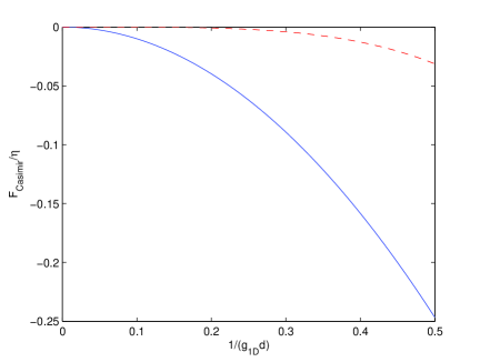
Figure 1: (Color online) The dependence of Casimir force on system length $d$ when $g_{1D}$ is fixed, where $\eta\equiv\pi\sqrt{2\rho}g_{1D}^{5/2}/12$ is the scale of force. The dash (red) line shows the Casimir force of a three dimensional interacting Bose gas without trap calculated in Ref. Roberts . The solid (blue) line shows the Casimir force of Bose gas in a strong harmonic trap as in equation (8).

If we restrict our system to be dilute and weakly interacting, the ground state energy can be calculated by the standard Bogoliubov method. The ground state energy of one dimensional Bose gas can be written as Lieb

$$E_{0}=\frac{N^{2}g_{1D}}{d}+\frac{1}{2}\sum_{p\neq 0}[\epsilon(p)-p^{2}-2\rho^{2}\gamma],$$ (4)

where $\epsilon(p)=\rho^{2}p\sqrt{p^{2}+4\gamma}$ is the elemental excitation spectrum of the quasi-one dimensional interacting Bose gas, $\rho=N/d$ is the number density of particles and $\gamma\equiv g_{1D}/2\rho$. It should be noted that $\epsilon(p)$ will give a phonon type excitation in the long wave-length limit which is very important to determine the low temperature property of the system. It is clear that the first term in equation (4) will just give a zero temperature classical pressure induced by the interaction between atoms which means that it has no contribution to the Casmir force. With the boundary condition $\varphi(0)=\varphi(d)$, the integral over $p$ will be replaced by a discrete summation. To calculate the Casimir force, we shall define the Casimir energy as the difference between the continuum form and the discrete form of the ground state energy

$$E_{Casimir}=\sum_{n=1}^{+\infty}f(n)-\int_{0}^{+\infty}f(n)dn+\frac{1}{2}f(0),$$ (5)

where $f(n)\equiv\varrho^{2}[\lambda n\sqrt{\lambda^{2}n^{2}+4\gamma}-\lambda^{2}n^{2}-2\gamma]$, $\lambda\equiv\!\pi/(\rho d)$ is just the discrete form of the second term in equation (4). The physical meaning of this definition embodies the contribution of the quantum fluctuation at zero temperature. By using the standard Euler-MacLaurin theorem Bordag , we can write the Casimir energy as

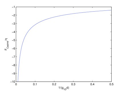
Figure 2: (Color online) The dependence of Casimir force on interacting strength $g_{1D}$ when length $d$ is fixed which has been shown in equation (8), where $\eta\equiv\pi\sqrt{2\rho}/(12d^{5/2})$ is the scale of force.

$$E_{Casimir}=\sum_{n=1}^{\infty}(-1)^{n}\frac{B_{2n}}{(2n)!}f^{2n-1}(0),$$ (6)

where $B_{2n}$ and $f^{2n-1}(0)$ , $n=1,2,3...$, are the Bernoulli numbers and the corresponding derivatives at zero point. By calculating equation (5) directly, we get the final result of the Casimir energy

$$E_{Casimir}\!=\!-\frac{\rho\pi\sqrt{\gamma}}{6}[\frac{1}{d}-\frac{1}{80g_{1D}d^{2}}+\mathscr{O}(d^{-3})],$$ (7)

and the Casimir force is

$$F_{Casimir}\!=\!-\frac{\partial E_{Casimir}}{\partial d}\!=\! - \frac{\rho\pi\sqrt{\gamma}}{6d^{2}}+\frac{\rho\pi\sqrt{\gamma}}{240g_{1D}d^{3}}$$ (8)

$$+ \mathscr{O}(d^{-4}).$$

we can see that the leading term of $F_{Casimir}$ is proportional to $d^{-2}$ which is sharply different with the case of three dimensional geometry Roberts , in which the Casimir force is proportional to $d^{-4}$ (see Fig. 1). It can be seen in Fig 1 that the Casimir force in three dimensional geomety decay much more rapidly than the quasi-one dimensional case as the system length increases. It means that the Casimir effect in one dimension may be easier to observe in experiments.

Through equation (8) and the expression of $g_{1D}$, it can be seen that it is possible to vary the Casimir force by tuning the the characteristic length of the harmonic potential $a_{\bot}$. We can also vary the interacting strength through Feshbach resonances which can be easily realized in experiments (see Fig. 2). We can see that the Casimir force increases rapidly when the interacting strength increases which is very reasonable because the interaction is the origin of quasi-particle fluctuation.

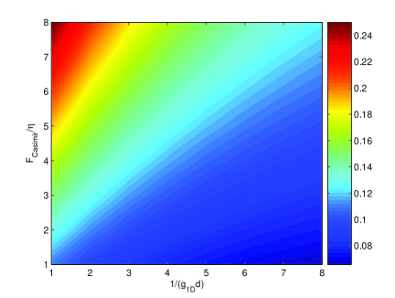
Figure 3: (Color online) The dependence on length $d$ and temperature $T$ of the Casimir force when $g_{1D}$ is fixed, where $\eta\equiv g_{1D}^{2}\upsilon_{s}\hbar$ is the scale of force, the temperature in the color bar is in unit of $g_{1D}\upsilon_{s}\hbar$. The color shows the temperature dependence. Blue (minimal temperature) and red (maximal temperature).

Furthermore, we will consider the contribution of thermal fluctuation to the Casimir effect. At finite temperature, the definition of Casimir force is generalized as Shyamal1

$$F_{Casimir}=-\frac{\partial}{\partial d}[\Omega_{T}(d)-\Omega_{T}(\infty)],$$ (9)

where $\Omega_{T}$ is the ground potential of our system at temperature T. In further calculation, we assume that the temperature is very low so that the quasi-particle energy spectrum can be approximated as $\varepsilon(p)=\upsilon_{s}p$ like a phonon, where $\upsilon_{s}=2\rho^{2}\sqrt{\gamma}$ is the speed of phonon. With this approximation, the system can be considered as a noninteracting phonon gas, therefore, the ground potential can be written as Pitaevskii

$$\Omega_{T}=-\frac{1}{\beta}\sum_{p}\ln\{1-\exp[-\beta\epsilon(p)]\},$$ (10)

where the form of $\epsilon(p)$ have been given above. If we take the boundary condition $\varphi(0)=\varphi(d)$ into consideration, the sum over $p$ in equation (9) will have the discrete form

$$\Omega_{T}(d)=-\frac{2}{\beta}\sum_{n=1}^{+\infty}\ln[1-\exp(-\lambda n)],$$ (11)

where $\lambda\equiv\frac{2\beta v_{s}\hbar}{d}=\frac{2\lambda_{T}}{d}$ and $\lambda_{T}$ is the thermal wave length of the phonon. In the thermodynamic limit, equation (9) will become a integral form

$$\Omega_{T}(\infty)=-\frac{2}{\beta}\int_{0}^{+\infty}\ln[1-\exp(-\lambda n)]dn=\frac{\pi^{2}}{3\lambda\beta}.$$ (12)

Analogous to the case of zero temperature, we also define the Casimir grand potential as

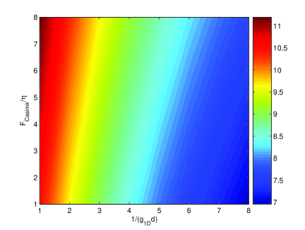
Figure 4: (Color online) The dependence on interacting strength $g_{1D}$ and temperature $T$ of the Casimir force when length $d$ is fixed, where $\eta\equiv\sqrt{2\rho}\rho\hbar/(6d^{\frac{5}{2}})$ is the scale of force, the temperature in the color bar is in unit of $\eta\equiv\sqrt{2\rho}\rho\hbar/(6d^{\frac{3}{2}})$. The color shows the temperature dependence. Blue (minimal temperature) and red (maximal temperature).

$$\Omega_{Casimir}\equiv\Omega_{T}(d)-\Omega_{T}(\infty),$$ (13)

and the Casimir force at finite temperature is

$$F_{Casimir}=-\frac{\partial}{\partial d}\Omega_{Casimir}.$$ (14)

In our calculation, we just consider the limit $\lambda\ll 1$. If the length of system $d$ is much larger than the thermal wave length $\lambda_{T}$ (which is mostly true under the real experimental conditions), this limit will always be satisfied. In this condition, we can expend the Casimir grand potential in powers of $\lambda$

$$\Omega_{Casimir}=\frac{2}{\beta}[\frac{1}{2}\ln\lambda-\frac{\lambda}{24}+\mathscr{O}(\lambda^{3})]+\mathcal{K}_{0},$$ (15)

where $\mathcal{K}_{0}=\frac{2}{\beta}(\sum_{n=2}^{+\infty}n!a_{n+2}-\frac{11}{12})$ is just a constant and has no contribution to the Casimir force. Then, the Casimir force can be derived as

$$F_{Casimir} = -\frac{\partial}{\partial d}\Omega_{Casimir}$$ (16)

$$= \frac{1}{d}[k_{B}T-\frac{v_{s}\hbar}{6d}+\mathscr{O}(\frac{1}{d^{3}})].$$

It is very interesting that the leading term of this force is positive which is contrast with the case of three dimensions Lev . We should also note that the method used to derive Casimir force at finite temperature is fundamentally different from the method in zero temperature, therefore the result of finite temperature cannot go back to the zero temperature solution when $T\rightarrow 0$. The dependence on length $d$, interacting strength $g_{1D}$ and temperature $T$ of the Casimir force is shown in Fig. 3 and Fig. 4. We can see that at fixed system length $d$ or interacting strength $g_{1D}$, the Casimir force increases with the temperature because more quasi-particles(phonons) will be excited by thermal fluctuation and contribute to the Casimir grand potential. We can also see that the Casimir force increases when the interacting strength $g_{1D}$ increases which means we can vary the force by tuning $g_{1D}$ through a Feshbach resonance.

To observe the Casimir effect described above, we consider an atomic-quantum-dot like configuration Recati ; Klein , which consists of single impurity atoms confined in a tight trap. In this configuration, the Casimir effect is represented as the interaction between the two trapped impurity atoms which can been seen as the boundary of the quasi-one dimensional bose gas Moritz ; Recati2 . The interacting energy can be measured by spectroscopy of a single trapped impurity atom as a function of the distance between the two impurity atoms. For a quantitative estimate of this effect, we compute the Casimir grand potential for typical experimental situations. For typical experimental consideration, the temperature can as low as 100 $nK$ and length of system is of order 1 $\mu m$, the sound velocity is of order 1 $cm/s$. Under these conditions, the Casimir grand potential in equation (15) is of order 100 $Hz$ which is experimentally accessible.

In conclusion, we have derived the formula of Casimir force of quasi-one dimensional Bose gas at zero and finite temperature. The results show that the Casimir force is very sensitive to the effective interacting strength which is related to the strength of the harmonic trapping potential. Another important point we found is that the Casimir force at finite temperature is positive which is opposite to the result of three dimensional case in earlier theoretical work Lev . The reason why this happens may be connected with the dimensional reduction effect in the condensed matter system. We also propose for the first time an experiment to control the Casimir force by tuning the frequency of the trapping potential which has not been considered in earlier experiments.

We express our appreciation for useful discussion with F. Zhou and S.Q. Shen. This work was supported in part by the project of knowledge innovation program (PKIP) of Chinese Academy of Sciences, by NSF of China under grant 10610335, 90406017, 60525417, 10574163, 90306016, the NKBRSF of China under Grant 2005CB724508 and 2006CB921400.

References

- (1) S.K. Lamoreaux, Phys. Rev. Lett. 78, 5 (1997).
- (2) U. Mohideen and A. Roy, Phys. Rev. Lett. 81, 4549 (1998).
- (3) L.P. Pitaevskii and S. Stringari, Phys. Rev. Lett. 81, 4541 (1999).
- (4) D.M. Stampur Kurn et al., Phys. Rev. Lett. 83, 2876 (1999).
- (5) M.Greiner et al., Nature 415, 39 (2002).
- (6) J.M. Vogels et al., Phys. Rev. Lett. 89, 020401 (2002).
-
(7)
S. Biswas, cond-mat/0702215;
cond-mat/0607412. - (8) A. Oshmyansky, cond-mat/0703211.
- (9) P.A. Martin et al., cond-mat/0507263.
- (10) M. Antezza et al., Phys. Rev. Lett. 97, 223203 (2006).
- (11) D.C. Roberts and Y. Pomeau, cond-mat/0503757 (2005).
- (12) A. Edery, J. Stat. Mech. P06007 (2006).
- (13) M. Olshanii, Phys. Rev. Lett. 81, 938 (1998).
-
(14)
L. Tonks, Phys. Rev. 50, 955 (1936);
M. Girardeau, J. Math. Phys. 1, 516 (1960);
M. D. Girardeau, Phys. Rev. 139, B500 (1965). - (15) E.H. Lieb and W. Lineger, Phys. Rev. 130, 1605 (1963).
- (16) A. Recati et al., Phys. Rev. A. 72, 023616 (2005).
- (17) M. Antezza et al., Phys. Rev. Lett. 95, 113202 (2005).
- (18) A. Recati et al., Phys. Rev. Lett. 94, 040404 (2005).
- (19) A. Klein, Phys. Rev. A. 71, 033605 (2005).
- (20) H. Moritz et al., Phys. Rev. Lett. 91, 250402 (2003).
- (21) M. Bordag et al., Phys. Rep. 353, 1 (2000).
- (22) L.P. Pitaevskii, Bose-Einstein Condensation (Clarendon Press, Oxford, 2003).