Equation of state for shock-compressed porous molybdenum from first-principles mean-field potential calculations

Abstract

The Hugoniot curves for shock-compressed molybdenum with initial porosities of 1.0, 1.26, 1.83, and 2.31 are theoretically investigated. The method of calculations combines the first-principles treatment for zero- and finite-temperature electronic contribution and the mean-field-potential approach for the ion-thermal contribution to the total free energy. Our calculated results reproduce the Hugoniot properties of porous molybdenum quite well. At low porosity, in particular, the calculations show a complete agreement with the experimental measurements over the full range of data. For the two large porosity values of 1.83 and 2.31, our results are well in accord with the experimental data points up to the particle velocity of 3.5 km/s, and tend to overestimate the shock-wave velocity and Hugoniot pressure when further increasing the particle velocity. In addition, the temperature along the principal Hugoniot is also extensively investigated for porous molybdenum.

Molybdenum (Mo) is a high technology metal with wide engineering applications for its thermal and mechanical strength, and also chemical resistances. It has been used as flyer and/or back reflector for shock wave experiments to provide accurate standard of high-pressure equation of state (EOS) Carter ; Mao . From this view, the precise EOS of Mo is critical for theoretical and practical implications. To obtain the EOS of Mo, the shock-compressed crystal Mo has been investigated by using different experiment systems Walsh ; McQueen ; Krupnikov ; McQueen1 ; Ragan ; Marsh ; Al ; Ragan1 ; Ragan2 ; Mitchell ; Hixson ; Trunin2 . The EOS shock-wave data have now been obtained at pressures ranging from 0.1 GPa up to a few TPa. Furthermore, to extend the EOS to regions of higher internal energy and temperature, the porous samples of Mo have also been experimentally investigated by Bakanova et al. Bakanova and Trunin et al. Trunin1 . Compared to the extensive theoretical calculations and analysis of the shock-compressed crystal Mo, the EOS shock-wave data of the porous Mo remain yet to be theoretically exploited and understood, which is a main driving force for our present study.

In this paper we calculate the Hugoniots of porous Mo with experimentally relevant Trunin1 ; Bakanova porosities $m$=1.0, 1.26, 1.83, and 2.31 using the mean-field potential (MFP) approach facilitated with the first-principles calculations. The MFP approach, which will be briefly described below, was initiated by Wang and co-workers Wang , and proved to provide a numerically convenient way to take into account the ion-thermal contribution in the total internal energy of the metal based on the first-principles calculation of zero-temperature internal energy. A lot of elemental metals have been successfully tested Wang ; Wang1 ; Wang ; Li ; Wang3 ; Wang4 ; Wang5 , and a general agreement between the MFP calculations and the experimental Hugoniots has been achieved under low shock temperatures (compared to the Fermi temperature $T_{F}$ of the valence electrons) and low Hugoniot pressures (typically within 0.1 TPa). Also, the shock-compressed porous carbon has been investigated using this approach Wang7 . Our present results of the Hugoniots for the porous Mo with different porosities show good agreement with the attainable experimental data from several groups.

Now we start with a brief review of the MFP approach. For a system with a given averaged atomic volume $V$ and temperature $T$, the Helmholtz free-energy $F(V,T)$ per atom can be written as

$$F(V,T)=E_{c}(V)+F_{ion}(V,T)+F_{el}(V,T),$$ (1)

where $E_{c}$ represents the 0-K total energy which is obtained from ab initio electronic structure calculations, $F_{el\text{ }}$is the free energy due to the thermal excitation of electrons, and $F_{ion}$ is the ionic vibrational free energy  which is evaluated from the partition function $Z_{ion}$=$\exp(-NF_{ion}/k_{B}T)$. Here $N$ is the total number of lattice ions. In the mean-field approximation, the classical $Z_{ion}$ is given by Wasserman

$$Z_{ion}=\left(\frac{mk_{B}T}{2\pi\hbar^{2}}\right)^{3N/2}\left(\int\exp\left(-g(\mathbf{r},V\right)/k_{B}T)d\mathbf{r}\right)^{N}.$$ (2)

The essential of the MFP approach is that the mean-field potential $g(\mathbf{r},V)$ is simply constructed in terms of $E_{c}$ as follows Wang

$$g(r,V)=\frac{1}{2}\left[E_{c}(R+r)+E_{c}(R-r)-2E_{c}(R)\right],$$ (3)

where $r$ represents the distance that the lattice ion deviates from its equilibrium position $R$. It should be mentioned that the well-known Dugdale-MacDonald expression Dug for the Grüneisen parameter can be derived by expanding $g(r,V)$ to order $r^{2}$. Then, $F_{ion}$ can be formulated as

$$F_{ion}(V,T)=-k_{B}T\left(\frac{3}{2}\ln\frac{mk_{B}T}{2\pi\hbar^{2}}+\ln v_{f}(V,T)\right),$$ (4)

with

$$v_{f}(V,T)=4\pi{\displaystyle\int}\exp\left(-\frac{g(r,V)}{k_{B}T}\right)r^{2}dr.$$ (5)

When the electron-phonon interaction and the magnetic contribution are neglected, the electronic contribution to the free energy is $F_{el}$=$E_{el}-TS_{el}$, where the bare electronic entropy $S_{el}$ takes the form Jarlborg

$$S_{el}(V,T)=-k_{B}{\displaystyle\int}n(\epsilon,V)\left[f\ln f+(1-f)\ln(1-f)\right]d\epsilon,$$ (6)

where $n(\epsilon,V)$ is the electronic density of states (DOS) and $f$ is the Fermi distribution function. With respect to Eq. (6), the energy $E_{el}$ due to electron excitations can be expressed as

$$E_{el}(V,T)=\int n(\epsilon,V)f\epsilon d\epsilon-\int^{\epsilon_{F}}n(\epsilon,V)\epsilon d\epsilon,$$ (7)

where $\epsilon_{F}$ is the Fermi energy. Given the Helmholtz free-energy $F(V,T)$, the other thermodynamic functions such as the entropy $S=-(\partial F/\partial T)_{V}$, the internal energy $E$=$F+TS$, the pressure $P$=$-(\partial F/\partial V)_{T}$, and the Gibbs free energy $G$=$F+PV$, can be readily calculated.

In all of our calculations we take the molybdenum structure to be body-centered-cubic (bcc) structure (Im3m). The 0-K total energy was calculated using the full-potential linearized augmented plane wave (LAPW) method Blaha in the generalized gradient approximation (GGA) Perdew . We used constant muffin-tin radii of 2.05$a_{0}$ ($a_{0}$ is the Bohr radius). The plane wave cutoff $K_{cut}$ is determined from $R_{mt}\times K_{cut}$=10.0. $4000$ $k$ points in the full zone are used for reciprocal-space integrations. The calculations were performed for atomic lattice parameter ranging from 4.8$a_{0}$ to 6.8$a_{0}$. For the highest calculated pressure the atomic volume has exceeded the touching sphere limit, an extrapolation for getting the 0-K total energy points by Morse function has been done.

The P-V Hugoniot was obtained from the Rankine-Hugoniot relation $P(V_{0}^{p}-V)/2$=$E-E_{0}^{p}$ for internal energy $E$, pressure $P$, and volume $V$, which are achieved by shock from initial conditions $V_{0}^{p}$ and $E_{0}^{p}$ for the present porous Mo. Usually, the density of porous materials of different porosities ($m<2\thicksim 3$) becomes at once the same as that of crystal under about 1.0 GPa shock-wave compression. In this case, it is a good approximation to take the initial internal energy $E_{0}^{p}$ for porous Mo to be exactly the same as the internal energy $E_{0}$ for crystal Mo. The $V_{0}^{p}$ is $V_{0}^{p}$=$mV_{0}$, where $m$ is the initial porosity and $V_{0}$ is the ambient volume of nonporous single-crystal Mo. Note that during the calculations, we have neglected shock melting and the phase dependence of the high-temperature equation of state, which is in accord with the finding of Mitchell et al. Mit1991 that the effects of shock melting on the $P$-$V$ Hugoniots of several reference metals were too weak to be observed.

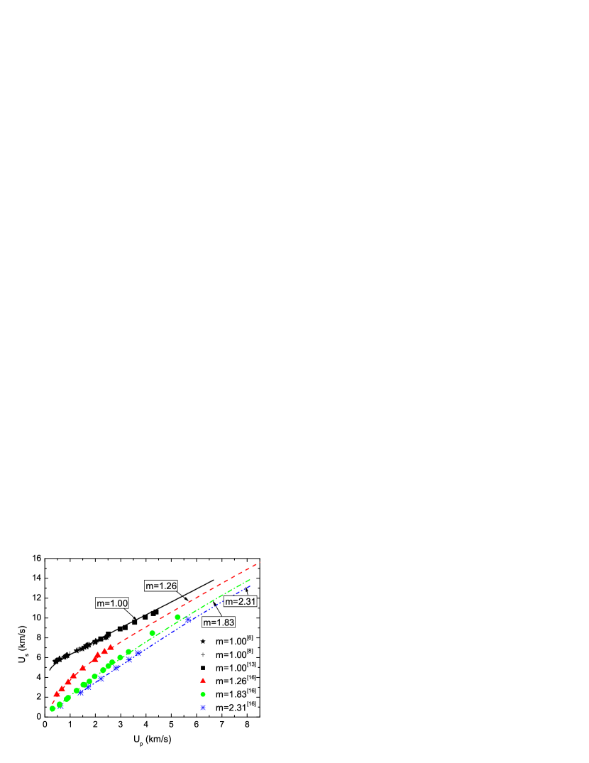
Figure 1: (Color online) Calculated shock-wave velocity versus particle velocity of molybdenum for initial porosities $m$=1.0, 1.26, 1.83, and 2.31. Different calculated curves represent different porosities. For comparison, the experimental data for $m$=1.0 (McQueen et al. McQueen1 , LASL Marsh , and Hixson et al. Hixson ), 1.26, 1.83, and $2.31$ (Trunin et al. Trunin1 ) are also shown in the figure.

Figure 1 shows the calculated results of $U_{p}$-$U_{s}$ diagram for $m$=1.0, 1.26, 1.83, and 2.31. Here $U_{p}$ is particle velocity and $U_{s}$ is shock-wave velocity. For comparison, the experimental data McQueen1 ; Marsh ; Hixson ; Trunin1 are also summarized in Fig. 1. For $m$=1.0 (crystal Mo), our calculated $U_{p}$-$U_{s}$ Hugoniot agrees well with the three groups of experimental data. Of these three groups of experimental data, the data points of McQueen et al. McQueen1 are obtained by using explosive system. The data points Marsh et al. Marsh (LASL Shock Hugoniot Data) are in the same particle velocity range from 0.4 to 2.5 km/s. The data points of Hixson et al. Hixson for $m$=1.0 are obtained by using the two-stage light-gas gun facility at Los Alamos National Laboratory (LANL) with $U_{p}$ ranging from 2.2 to 4.4 km/s. The least-squares fit to these three groups of data gives the relation $U_{s}$=5.109$+$1.247$U_{p}$ at $m$=1.0, while our calculated results gives $U_{s}$=4.915$+$1.347$U_{p}$. For $m$=1.26, it reveals in Fig. 1 that our calculated $U_{s}$ versus $U_{p}$ relation agrees with the data points of Trunin et al. Trunin1 very well. For the two larger porosities $m$=1.83 and $m$=2.31, our results agree well with the data points of Trunin et al. Trunin1 up to the particle velocity of $3.5$ km/s. At even more higher particle velocity ($U_{p}>$4.0 km/s), the scarce attainable experimental data for $m$=1.83 and $m$=2.31 show that the amplitude of the shock-wave velocity is underestimated by our calculations, and this deviation seems to be growing with increasing the particle velocity.

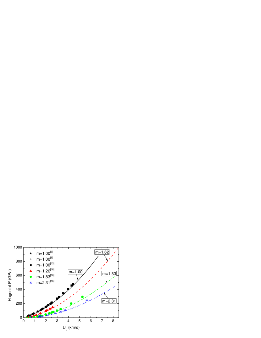
Figure 2: (Color online) Calculated Hugoniot pressure versus particle velocity of molybdenum for initial porosities $m$=1.0, 1.26, 1.83, and 2.31. The experimental data points from several groups are also shown in the same way as occurred in Fig. 1.

Figure 2 shows the calculated Hugoniot pressures as functions of the particle velocity $U_{p}$ for different porosities. The experimental data McQueen1 ; Marsh ; Hixson ; Trunin1 are also plotted for comparison. For crystal Mo at equilibrium, i.e., $m$=1.0, one can see that the theory agrees well with the experiments over the full range of data. For $m$=1.26, our calculated results are also in excellent agreement with the experiment by Trunin et al. Trunin1 . Note that for this porosity, there still lacks the data points at high pressure, and our calculation above the pressure of 147 GPa needs to be experimentally verified in the future. For $m$=1.83 and 2.31, our results agree well with the experimental data points up to the Hugoniot pressure of 100 GPa. With further increase of the particle velocity, a slight deviation of the present calculated Hugoniot pressure from the measurement occurs, with the latter systematically larger than the former at given $U_{p}$.

Figure 3 shows our results of pressure dependence of Hugoniot volume (scaled by ambient atomic volume $V_{0}$ of the crystal Mo) for different porosities. Again, the attainable experimental data McQueen1 ; Marsh ; Hixson ; Trunin1 are also illustrated in Fig. 3 for comparison. For $m$=1.0 and 1.26, the agreement between our calculated results and experimental measurement is obviously good. For the porosities $m$=1.83 and 2.31, on the other side, the experimental points become scattered and are difficult to fit in a smooth curve. For this reason, the difference between our calculated $V$-$P$ relation and the experimental data is somewhat enlarged compared to the $U_{p}$-$U_{s}$ and $U_{p}$-$P$ relations. The scattering of data points is most likely due to the fact that it is more difficult for larger porosity to prepare the samples with the same initial porosity for several experiments. It should be mentioned that the $V$-$P$ relation is more sensitive to the difference between theoretical results and experimental points than that of $U_{p}$-$U_{s}$ and $U_{p}$-$P$ relations.

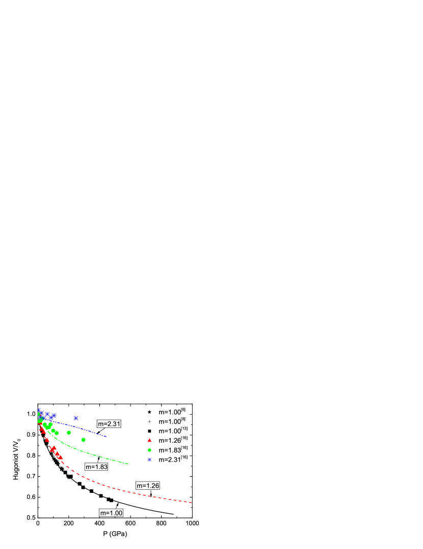
Figure 3: (Color online) Calculated Hugoniot pressure versus relative atomic volume of molybdenum for initial porosities $m$=1.0, 1.26, 1.83, and 2.31. The experimental data points from several groups are also shown in the same way as occurred in Fig. 1.

The calculated Hugoniot temperature is shown in Fig. 4 as a function of pressure $P$ for several values of porosity. For comparison, the previous calculations by McQueen et al. McQueen and Hixson et al. Hixson for the case of $m$=1.0 are also shown in Fig. 4. Clearly, our results for $m$=1.0 is in good agreement with the previous results. One can see from Fig. 4 that the larger the initial porosity is, the steeper the temperature curve is. This is due to that the porous material can absorb and transform to heat the energy of shock-wave in the process of shock compression.

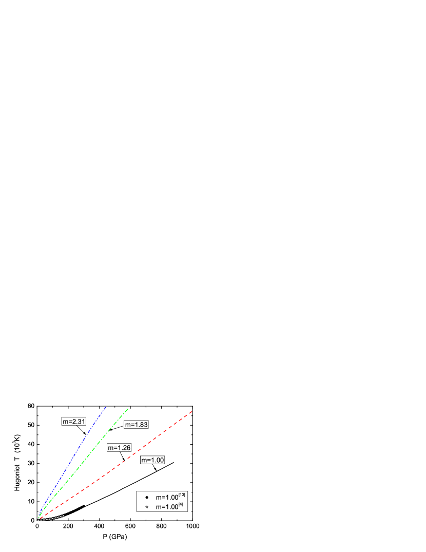
Figure 4: (Color online) Calculated Hugoniot temperatures as functions of Hugoniot pressure $P$ for molybdenum with initial porosities $m$=1.0, 1.26, 1.83, and 2.31. The filled circle and the star points represent theoretical results of McQueen et al. McQueen and Hixson et al. Hixson , respectively.

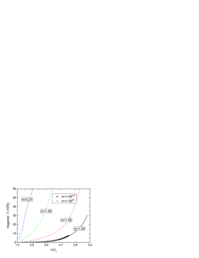
Figure 5: (Color online) Hugoniot temperature versus relative volume of molybdenum for initial porosities $m$=1.0, 1.26, 1.83, and 2.31. The filled circle and star points represent theoretical results of McQueen et al. McQueen and Hixson et al. Hixson , respectively.

Finally, figure 5 shows the calculated Hugoniot temperature as a function of atomic volume for the values of $m$=1.00, 1.26, 1.83, and 2.31. The previous theoretical results McQueen ; Hixson for $m$=1.0 are also plotted in Fig. 5 for comparison. The agreement between our results and those of the two groups McQueen ; Hixson is very good. Due to the reason mentioned above, the Hugoniot temperature increases rapidly with the increase of initial porosity at a given relative volume of Mo.

In summary, the Hugoniots of Mo with porosities $m$=1.0, 1.26, 1.83, and 2.31 have been calculated by using the first-principles MFP approach. Our results show good agreement with the experimental data at $m$=1.00 and 1.26. For larger porosities of $m$=1.83 and 2.31, the difference between our results and data points grows with the pressure. The Hugoniot temperature of porous Mo have also been calculated. For $m$=1.0, our calculated results are remarkably consistent with the previous calculations. At present, there are no measurement of Hugoniot temperature attainable for porous Mo to confirm our theoretical results, and we leave this verification for the future shock-wave experiments.

This work was partially supported by NSFC under grant number 10604010 and 10544004.

References

- (1) W. J. Carter, S. P. Marsh, J. N. Fritz, and R. G. McQueen, NBS. Spec. Pub1. 36, 147 (1971).
- (2) H. K. Mao, P. M. Bell, J. W. Shaner, and D. J. Steinberg, J. Appl. Phys. 49, 3276 (1978).
- (3) J. M. Walsh, M. H. Rice, R. G. Mcqueen, and F. L. Yarger, Phys. Rev. 108, 196 (1957).
- (4) R. G. McQueen, and S. P. Marsh, J. Appl. Phys. 31, 1253 (1960).
- (5) K. K. Krupnikov, A. A. Bakanova, M. I. Brazhnik, and R. F. Trunin, Dokl. Akad. Nauk SSSR 148, 1302 (1963) [in Russian] (Sov.Phys. - Dokl. 8, 205 (1963)).
- (6) R. G. McQueen, S. P. Marsh, J. W. Taylor, J. N. Fritz, and W. J. Carter, The equation of state of solids from shock wave studies. - In: High Velocity Impact Phenomena edited by R. Kinslow (Academic Press, New York, 1970).
- (7) C. E. Ragan, M. G. Silbert, and B. C. Diven, J. Appl. Phys. 48, 2860 (1977).
- (8) Los Alamos Shock Hugoniot Data, edited by S. P. Marsh (University of California, Berkeley, 1980).
- (9) L. V. Al’tshuler, A. A. Bakanova, I. P. Dudoladov, E. A. Dynin, R. F. Trunin, and B. S. Chekin, Zh. Prikl. Mekh. Tekhn. Fiz. 2, 3 (1981) [in Russian] (J. Appl. Mech. Techn. Phys. 22, 145 (1981)).
- (10) C. E. Ragan, Phys. Rev. A 25, 3360 (1982).
- (11) C. E. Ragan, Phys. Rev. A 29, 1391 (1984).
- (12) A. C. Mitchell, W. J. Nellis, J. A. Moriarty, R. A. Heinle, N. C. Holmes, R. E. Tipton, and G. W. Repp, J. Appl. Phys., 69, 2981 (1991).
- (13) R. S. Hixson, and J. N. Fritz, J. Appl. Phys. 71, 1721 (1992).
- (14) R. F. Trunin, N. V. Panov, A. B. Medvedev, Pis’ma Zh. Eksp. Teor. Fiz. 62, 572 (1995) [in Russian].
- (15) A. A. Bakanova, I. P. Dudoladov, and Yu. N. Sutulov, Zh. Prikl. Mekh. Tekhn. Fiz. 2, 117-122 (1974) [in Russian] (J. Appl. Mech. Techn. Phys. 15, 241 (1974)).
- (16) R. F. Trunin, G. V. Simakov, Yu. N. Sutulov, A. B. Medvedev, B. D. Rogozkin, and Yu. E. Fedorov, Zh. Eksp. Teor. Fiz. 96, 1024 (1989) [in Russian] (Sov. Phys. - JETP 69, 580-588 (1989)).
- (17) Y. Wang, D. Chen, and X. Zhang, Phys. Rev. Lett. 84, 3220 (2000).
- (18) Y. Wang, Phys. Rev. B 61, R11863 (2000).
- (19) L. Li and Y. Wang, Phys. Rev. B 63, 245108 (2001).
- (20) Y. Wang and Y. F. Sun, Chin. Phys. Lett. 18, 864 (2001).
- (21) Y. Wang, R. Ahuja, and B. Johansson, J. Phys.: Condens. Matter 14, 10895 (2002).
- (22) Y. Wang, R. Ahuja, and B. Johansson, High Press. Res. 22, 485 (2002).
- (23) Y. Wang, Z.-K. Liu, L.-Q. Chen, L. Burakovsky, D. L. Preston, W. Luo, B. Johansson, and R. Ahuja, Phys. Rev. B 71,054110 (2005).
- (24) E. Wasserman, L. Stixrude, and R.E. Cohen, Phys. Rev. B 53, 8296 (1996).
- (25) J. S. Dugdale and D. K. C. MacDonald, Phys. Rev. 89, 832 (1953).
- (26) T. Jarlborg, E. G. Moroni, and G. Grimvall, Phys. Rev. B 55, 1288 (1997).
- (27) P. Blaha, K. Schwarz, G. Madsen, D. Kvasnicka, and J. Luitz, WIEN2K, http://www.wien2k.at/
- (28) P. Perdew, K. Burke, and M. Ernzerhof, Phys. Rev. Lett. 77, 3865 (1996).
- (29) A. C. Mitchell, W. J. Nellis, J. A. Moriarty, R. A. Heinle, N. C. Holmes, R. E. Tipton, and G. W. Repp, J. Appl. Phys. 69, 2981 (1991).