Control of spin coherence in semiconductor double quantum dots

Abstract

We propose a scheme to manipulate the spin coherence in vertically coupled GaAs double quantum dots. Up to ten orders of magnitude variation of the spin relaxation and two orders of magnitude variation of the spin dephasing can be achieved by a small gate voltage applied vertically on the double dot. Specially, large variation of spin relaxation still exists at $0$ K. In the calculation, the equation-of-motion approach is applied to obtain the electron decoherence time and all the relevant spin decoherence mechanisms, such as the spin-orbit coupling together with the electron–bulk-phonon scattering, the direct spin-phonon coupling due to the phonon-induced strain, the hyperfine interaction and the second-order process of electron-phonon scattering combined with the hyperfine interaction, are included. The condition to obtain the large variations of spin coherence is also addressed.

I Introduction

The fast development of spintronics aims at making devices based on the electron spin. Semiconductor quantum dots (QDs) are one of the promising candidates for the implementation of quantum computationsAwschalom ; Hans ; Loss ; Taylor0 because of the relative long spin coherence time, which has been proved both theoreticallyJiang2 ; Semenov and experimentally.Hanson ; Amasha ; Petta Among different kinds of QDs, double quantum dot (DQD) system attracted much more attention recently as there is an additional coupling between two QDs in both verticalPi ; Ono ; Austing and parallelPetta ; Koppens ; Laird ; jaro DQDs, which can be controlled conveniently by a small gate voltage. Therefore spin devices based on DQDs can be designed with more flexibility. So far many elements of the spintronic device, such as quantum logical gates,Mason ; Hanson2 spin filtersCota ; Mireles and spin pumpsCota were proposed and/or demonstrated based on DQD system. Specially, in our previous work, a way to control spin relaxation time ($T_{1}$) induced by the spin-orbit coupling (SOC) together with the electron–bulk-phonon (BP) scattering in DQDs by a small gate voltage was proposed.Wang However, according to our latest study,Jiang2 the spin relaxation can be controlled by other mechanisms also, if calculated correctly. In the present paper, we include all the spin decoherence mechanisms following our latest study in the single QD system, and apply the equation-of-motion approach to study the spin decoherence in DQD system. By this approach, not only the spin relaxation time but also the spin dephasing time ($T_{2}$) can be obtained. We show that both the spin relaxation and the spin dephasing can be manipulated by a small gate voltage in DQD system. Especially, the large variation of spin relaxation still exists even at $0$ K. The DQD system studied here can be realized easily using the present available technology.

We organize the paper as following. In Sec. II we set up the model and briefly introduce different spin decoherence mechanisms. The equation-of-motion approach is also explained simply. Then in Sec. III we present our numerical results. We first show how the eigen energies and eigen wave functions vary with the bias field in Sec. IIIA. Then the electric field dependences of spin relaxation and spin dephasing are shown in Sec. IIIB and IIIC, respectively. We conclude in Sec. IV.

II Model and Method

We consider a single electron spin in two vertically coupled QDs with a bias voltage $V_{d}$ and an external magnetic field ${\mathbf{B}}$ applied along the growth direction ($z$-axis). Each QD is confined by a parabolic potential $V_{c}({\bf r})=\frac{1}{2}m^{\ast}\omega_{0}^{2}{\bf r}^{2}$ (therefore the effective dot diameter $d_{0}=\sqrt{\hbar\pi/m^{\ast}\omega_{0}}$) in the $x$-$y$ plane in a quantum well of width $d$. The confining potential $V_{z}(z)$ along the $z$-direction reads

$$V_{z}(z)=\begin{cases}eEz+\frac{1}{2}eV_{d},&\frac{1}{2}a<|z|<\frac{1}{2}a+d\\ eEz+\frac{1}{2}eV_{d}+V_{0},&|z|\leqslant\frac{1}{2}a\\ \infty,&\mbox{otherwise}\end{cases}\ ,$$ (1)

in which $V_{0}$ represents the barrier height between the two dots, $a$ stands for the inter-dot distance and $E=V_{d}/(a+2d)$ denotes the electric field due to the bias voltage $V_{d}$. Then the electron Hamiltonian reads $H_{e}=\mathbf{P}^{2}/(2m^{\ast})+V_{c}({\mathbf{r}})+V_{z}(z)+H_{Z}+H_{SO}$, where $m^{\ast}$ is the electron effective mass and $\mathbf{P}=-i\hbar\mathbf{\nabla}+\frac{e}{c}\bf{A}$ with ${\mathbf{A}}=(B/2)(-y,x,0)$ being the vector potential. $H_{Z}=\frac{1}{2}g\mu_{B}B\sigma_{z}$ is the Zeeman energy with $g$, $\mu_{B}$ and $\sigma$ being the $g$-factor of electron, Bohr magneton and Pauli matrix respectively. $H_{so}$ is the Hamiltonian of the SOC. In GaAs, when the quantum well width and the gate voltage along the growth direction are small, the Rashba SOCYu is unimportant.flat Therefore, only the Dresselhaus termDresselhaus contributes to $H_{SO}$. When the quantum well width is smaller than the QD diameter, the dominant term in the Dresselhaus SOC reads $H_{so}=\frac{1}{\hbar}\sum_{\lambda}\gamma_{\lambda}^{\ast}(-P_{x}\sigma_{x}+P_{y}\sigma_{y})$, with $\gamma_{\lambda}^{\ast}=\gamma_{0}\langle P_{z}^{2}\rangle/\hbar^{2}$. $\gamma_{0}$ denotes the Dresselhaus coefficient, $\lambda$ is the quantum number of $z$-direction and $\langle P_{z}^{2}\rangle_{\lambda}\equiv-\hbar^{2}\int\psi_{z,\lambda}^{\ast}(z)\partial^{2}/\partial z^{2}\psi_{z,\lambda}(z)dz$, where $\psi_{z,\lambda}$ ($\lambda=1,2,3\cdots$) is the eigen wave function of the electron along the $z$-direction.Wang The electron eigen energy and wave function in the $x$-$y$–plane can be obtained by the exact diagonalization approach.Cheng

The interactions between the electron and the lattice lead to the electron spin decoherence. These interactions contain two parts, one is the hyperfine interaction between the electron and the nuclei, the other is the electron-phonon interaction which is further composed of the electron-BP interaction $H_{ep}$, the direct spin-phonon coupling due to the phonon induced strain $H_{strain}$ and the phonon-induced $g$-factor fluctuation. We briefly summarize these spin decoherence mechanisms and the detailed expressions can be found in Ref. Jiang2, : (i) The SOC together with the electron-BP scattering $H_{ep}$. As the SOC mixes different spins, the electron-BP can induce spin relaxation and spin dephasing. (ii) Direct spin-phonon coupling due to the phonon-induced stain $H_{strain}$.Dyakonov Because this mechanism mixes different spins and also is related to the electron-phonon interaction, it can induce spin decoherence alone. (iii) The hyperfine interaction $H_{eI}$.Abragam It is noted that the hyperfine interaction alone only induces $T_{2}$ since it only changes the electron spin, but not the electron energy. (iv) The second-order process of hyperfine interaction combined with the electron-BP interaction $V_{eI-ph}^{(3)}=|\ell_{2}\rangle[\sum_{m\not=\ell_{1}}(\langle\ell_{2}|H_{ep}|m\rangle\langle m|{H_{eI}({\mathbf{r}})}|\ell_{1}\rangle)/(\varepsilon_{\ell_{1}}-\varepsilon_{m})+\sum_{m\not=\ell_{2}}(\langle\ell_{2}|{H_{eI}({\mathbf{r}})}|m\rangle\langle m|H_{ep}|\ell_{1}\rangle)/(\varepsilon_{\ell_{2}}-\varepsilon_{m})]\langle\ell_{1}|$, where $|\ell_{i}\rangle$ ($i=1,2,3\cdots$) and $\varepsilon_{\ell_{i}}$ are the eigen state and eigen energy of $H_{e}$, respectively. Although the hyperfine interaction can not induce $T_{1}$ alone, it is noted that the second-order process, combined with the electron-BP interaction, can induce both $T_{1}$ and $T_{2}$. The other mechanisms, including the first-order process of hyperfine interaction combined with the electron-BP scatteringAbalmassov and the $g$-factor fluctuationRoth have been proved to be negligible.Jiang2

Due to the SOC, all the states are impure spin states with different expectation values of the spin. For finite temperature, the electron is distributed over many states and therefore one has to average over all the involved processes to obtain the total spin relaxation time. The Fermi-Golden-Rule approach calculates the spin relaxation from the initial state to the final one whose majority spin polarizations are opposite. However, the average method is inadequate when many impure states are included.Jiang2 Also the Fermi-Golden-Rule approach can not be used to calculate the spin dephasing time. Therefore, in this paper we adopt the equation-of-motion approach for many-level system with Born approximation developed in Ref. Jiang2, . When the spin dephasing induced by the hyperfine interaction is considered, as the slow relaxation of nuclear bath compared to the electron, the kinetics is non-Markovian. Moreover, because of the Born approximation, this equation-of-motion approach can only be applied for strong magnetic field ($\geq 3.5$ T).Coish Therefore, the pair-correlation methodYao is further adopted to calculate the hyperfine interaction induced $T_{2}$ for small magnetic field. What should be emphasized is that the SOC is always included, no matter which mechanism is considered. It has been shown that its effect to spin decoherence can not be neglected.Jiang2

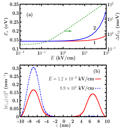
Figure 1: (Color on line) (a) The Lowest two eigen energies along the $z$-axis ${\cal E}_{\lambda}$ ($\lambda=1,2$) and the energy difference $\Delta{\cal E}_{12}={\cal E}_{2}-{\cal E}_{1}$ vs. the bias field $E$. Note the scale of $\Delta{\cal E}_{12}$ is on the right side of the figure. (b) Square of the absolute value of the ground state wave function along the $z$-axis at two typical bias fields. In the calculation, the well width $d=5$ nm, the inter-dot distance $a=10$ nm and the barrier height $V_{0}=0.4$ eV.

III Numerical Results

Following the method addressed above, we perform the numerical calculation in a typical vertically coupled GaAs DQD with barrier height $V_{0}=0.4$ eV, inter-dot distance $a=10$ nm and well width $d=5$ nm. The GaAs material parameters and the parameters related to different mechanisms are the same with those in Ref. Jiang2, .

III.1 Electric field dependence of eigen energy and eigen wave function along $z$-axis

The eigen energy and eigen wave function along the $z$-direction are obtained numerically. In Fig. 1(a), the lowest two eigen energies ${\cal E}_{1}$ and ${\cal E}_{2}$ along the $z$-axis and their difference $\Delta{\cal E}_{12}={\cal E}_{2}-{\cal E}_{1}$ are plotted as functions of the electric field $E$. It can be seen that the energy difference $\Delta{\cal E}_{12}$ increases quickly with the electric field $E$ when $E$ is larger than $0.1$ kV/cm. The eigen wave function of the ground state along the $z$-axis also has large variation with $E$. It can be seen clearly in Fig. 1(b) that when $E$ is very small ($1.2\times 10^{-2}$ kV/cm), the wave function of the ground state locates at the two wells almost equally. However, when $E$ is large enough ($89$ kV/cm), the wave function of the ground state locates mostly at the quantum well with lower potential. The physics of such bias-voltage-induced quick change of eigen energy and eigen wave function can be understood as what follows. Because of the large barrier height $V_{0}$ and/or large inter-dot distance $a$, the two quantum dots are nearly independent and the eigen wave function along the $z$-axis of the lowest subband spreads equally over the two QDs when the source-drain voltage is very small. Therefore at this time the energy difference between the lowest two energy levels along the $z$-axis $\Delta{\cal E}_{12}$ is very small. However, with the increase of the source-drain voltage, electron can tunnel through the barrier and the wave function is almost located at one dot with lower potential and therefore $\Delta{\cal E}_{12}$ increases quickly with $E$.

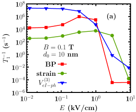
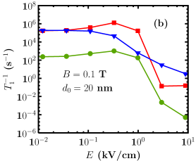
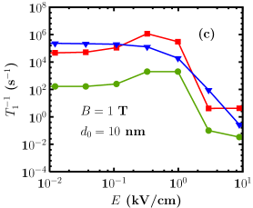
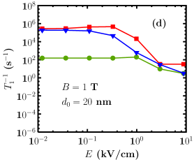
Figure 2: (Color on line) $T_{1}^{-1}$ induced by different mechanisms vs. the electric field at different magnetic fields and dot diameters. $T=4$ K. Curves with $\blacksquare$: by SOC together with the electron-BP scattering; Curves with $\bullet$: by the direct spin-phonon coupling due to the phonon-induced strain; Curves with $\blacktriangledown$: by the second-order process of the hyperfine interaction together with the BP ($V_{eI-ph}^{(3)}$).

III.2 Spin relaxation time $T_{1}$ vs. Electric field $E$

The spin relaxation due to various mechanisms at different magnetic fields $B$ and quantum dot diameters $d_{0}$ are plotted as functions of electric field $E$ in Fig. 2. The temperature $T=4$ K. It is seen that with the increase of $E$, the spin relaxations induced by all the three mechanisms almost keep unchanged for small $E$ (when $E<0.1$ kV/cm), then increase a little and reach maximums around $0.3$ kV/cm. What is interesting is that when $E$ is increased to around $1.1$ kV/cm, the spin relaxations are suppressed very quickly over a small window of $E$. Therefore, the total spin relaxation can be controlled effectively with a small value of the variation of the bias field $\Delta E$. For example, in Fig. 2(a), the spin relaxation shows ten orders of magnitude variation when the electric field $E$ changes from $0.1$ to $10$ kV/cm. This can be understood as following. All the three mechanisms are related to the electron-BP scattering which is affected sensitively by the phonon wave length. The scattering becomes most efficient when the phonon wave length is comparable with the dot size. It is also known that the spin relaxations between the first and second subband are dominant for small electric field.Wang Therefore when $E<0.1$ kV/cm, as the energy difference between the lowest two subband along the $z$-direction $\Delta{\cal E}_{12}$ is almost constant (see Fig. 1 (a)), the spin relaxation keeps nearly unchanged. When the phonon wave length is comparable with the dot size, the electron-phonon scattering becomes most efficient. Therefore the spin relaxations show maximums. However, with the further increase of energy difference $\Delta{\cal E}_{12}$ by the bias voltage, the phonon wave length becomes larger than the dot size. Consequently the spin relaxation decreases very quickly over a small window of $\Delta E$.

Now we focus on the variation magnitude of the spin relaxation with the bias field under different conditions. The largest variation of $T_{1}$ ($10$ orders of magnitude) happens at small magnetic field $B=0.1$ T and small diameter $d_{0}=10$ nm. However, for larger $d_{0}$ ($20$ nm in Fig. 2(b)) or larger $B$ ($1$ T in Fig. 2(c)), the variations of the total spin relaxation decrease by several orders of magnitude. It is further seen that when both $d_{0}$ and $B$ are increased [$d_{0}=20$ nm and $B=1$ T in Fig. 2(d)], the variations of the total spin relaxation is even smaller. This is because the spin relaxation induced by the electron-BP interaction and $V_{eI-ph}^{(3)}$ decreases with $B$ and $d_{0}$ in the high electric field region, where electron is mostly confined in one dot. This is similar to the single QD case.Jiang2 Therefore to achieve large control of spin decoherence, the magnetic field $B$ and dot diameter $d_{0}$ should be small.

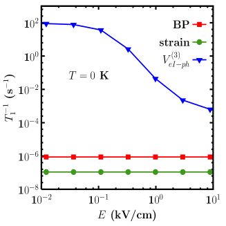
Figure 3: (Color on line) $T_{1}^{-1}$ induced by different mechanisms vs. the electric field. In the calculation, $d_{0}=10$ nm, $B=0.1$ T and $T=0$ K. Curve with $\blacksquare$: by SOC together with the electron-BP scattering; Curve with $\bullet$: by the direct spin-phonon coupling due to the phonon-induced strain; Curve with $\blacktriangledown$: by the second-order process of the hyperfine interaction together with the BP ($V_{eI-ph}^{(3)}$).

We further investigate the electric field dependence of spin relaxation at $T=0$ K and the results are shown in Fig. 3. It is interesting to see that the spin relaxation induced by the second-order process of hyperfine interaction combined with the electron-BP scattering ($V_{eI-ph}^{(3)}$) still has large variation with $E$ ($5$ orders of magnitude variation when $E$ changes from $0.1$ to $10$ kV/cm). However, the spin relaxations induced by the other two mechanisms keep almost unchanged. This is because when $T=0$ K, the electron only locates at the lowest orbital level and the spin relaxation happens only between the lowest two Zeeman sublevels which keeps unchanged with $E$. Therefore the large variations of spin relaxations induced by the SOC together with the electron-BP scattering and the strain-induced direct spin-phonon coupling no longer exist. However, for $V_{eI-ph}^{(3)}$, which is the second-order process scattering, the middle states $|m\rangle$ can be higher levels as the hyperfine interaction can couple the spin-opposite states in different subband along the $z$-axis. The energy differences between the middle states and the initial/final states increase with $E$ and therefore the spin relaxation induced by $V_{eI-ph}^{(3)}$ decreases with $E$ quickly.

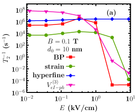
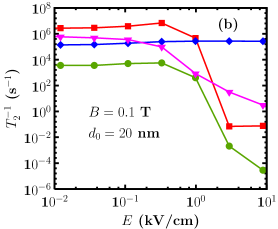
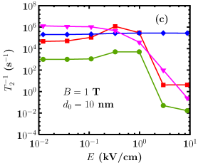
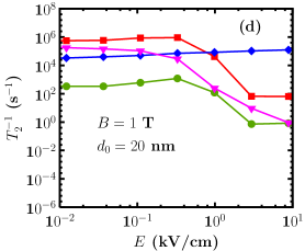
Figure 4: (Color on line) $T_{1}^{-1}$ and $T_{2}^{-1}$ induced by different mechanisms vs. the electric field at different magnetic fields and dot diameters. $T=4$ K. Curves with $\blacksquare$: by SOC together with the electron-BP scattering; Curves with $\bullet$: by the direct spin-phonon coupling due to the phonon-induced strain; Curves with $\blacktriangledown$: by the second-order process of the hyperfine interaction together with the BP ($V_{eI-ph}^{(3)}$); Curves with $\blacklozenge$: by the hyperfine interaction.

III.3 Spin dephasing time $T_{2}$ vs. Electric field $E$

Now we turn to study the variation of spin dephasing with the electric field $E$ and the results under different conditions are summarized in Fig. 4. It is seen that the spin dephasing induced by the SOC together with the electron-BP scattering, direct spin-phonon coupling due to the phonon-induced strain and the second-order process of electron-BP scattering combined with the hyperfine interaction always has several orders of magnitude variation with $E$ at different $d_{0}$ and $B$. However, the spin dephasing induced by the hyperfine interaction only increases a little with $E$, which suppresses the large variation of the spin dephasing induced by the other three mechanisms. Nevertheless, there is still two orders of magnitude variation of the spin dephasing when $B$ and $d_{0}$ are small (Fig 4(a)). The large variation of spin dephasing induced by the three mechanisms related to electron-phonon scattering comes from the fast increase of the energy difference $\Delta{\cal E}_{12}$, similar to the analysis of spin relaxation. The spin dephasing induced by the hyperfine interaction is not so sensitive with $E$. This is because for the hyperfine interaction, $T_{2}\approx E_{z}A^{-2}N$, which is obtained from the pair-correlation approach, with $E_{z}$, $A$ and $N$ being the Zeeman splitting energy, the hyperfine interaction parameter and the nuclear number in the quantum dot respectively.Yao With the increase of the electric field $E$, $E_{z}$ and $A$ keep unchanged and the wave function of the ground state is gradually localized on one dot with lower potential. This means the effective quantum dot size decreases and consequently $N$ decreases. However, as the effective quantum dot size decreases from two dots into one dot with the bias field $E$, $N$ for large $E$ is only about a half of that for small $E$. Therefore, $T_{2}^{-1}$ for large field is about two times of that for small field due to the decrease of $N$. However, this increase of $T_{2}^{-1}$ induced by the hyperfine interaction is very small compared to that induced by other three mechanisms (which have several orders of magnitude variation). What should be pointed out is that the variation of spin dephasing does not exist at $T=0$ K. This is because the hyperfine interaction is dominant for the spin dephasing at $T=0$ K, which keeps unchanged with $E$.

IV Conclusion

In conclusion, we propose a scheme to manipulate the spin decoherence (both $T_{1}$ and $T_{2}$) in DQD system by a small gate voltage. Up to ten orders of magnitude of spin relaxation and up to two orders of magnitude of spin dephasing can be obtained. To obtain large variation of spin decoherence, the inter-dot distance and/or the barrier hight should be large enough in order to guarantee that the two QDs are nearly independent for the small bias voltage. At the same time, the effective diameter and magnetic field should be small to get as large variation as possible. Finally, based on the present available experimental technology, the DQD system applied in this paper can be realized easily.Ono ; Austing

- (1) Semiconductor Spintronics and Quantum Computation, edited by D. D. Awschalom, D. Loss, and N. Samarth (Springer-Verlag, Berlin, 2002); I. Zutic, J. Fabian, and S. Das Sarma, Rev. Mod. Phys. 76, 323 (2004); R. Hanson, L. P. Kouwenhoven, J. R. Petta, S. Tarucha, and L. M. K. Vandersypen, Rev. Mod. Phys. 79, 1217 (2007); J. Fabian, A. Matos-Abiague, C. Ertler, P. Stano, and I. Zutić, acta physica slovaca 57, 565 (2007).
- (2) H.-A. Engel, L. P. Kouwenhoven, D. Loss, and C. M. Marcus, Quantum Information Processing 3, 115 (2004); D. Heiss, M. Kroutvar, J. J. Finley, and G. Abstreiter, Solid State Commun. 135, 591 (2005); and references therein.
- (3) D. Loss and D. P. DiVincenzo, Phys. Rev. A 57, 120 (1998).
- (4) J. M. Taylor, H.-A. Engel, W. Dür, A. Yacoby, C. M. Marcus, P. Zoller, and M. D. Lukin, Nature Phys. 1, 177 (2005).
- (5) J. H. Jiang, Y. Y. Wang, and M. W. Wu, Phys. Rev. B 77, 035323 (2008).
- (6) Y. G. Semenov and K. W. Kim, Phys. Rev. B 75, 195342 (2007).
- (7) R. Hanson, B. Witkamp, L. M. K. Vandersypen, L. H. W. van Beveren, J. M. Elzerman, and L. P. Kouwenhoven, Phys. Rev. Lett. 91, 196802 (2003).
- (8) S. Amasha, K. MacLean, I. Radu, D. M. Zumbühl, M. A. Kastner, M. P. Hanson, and A. C. Gossard, arXiv:cond-mat/0607110.
- (9) J. R. Petta, A. C. Johnson, J. M. Taylor, E. A. Laird, A. Yacoby, M. D. Lukin, C. M. Marcus, M. P. Hanson, and A. C. Gossard, Science 309, 2180 (2005).
- (10) M. Pi, A. Emperador, M. Barranco, F. Garcias, K. Muraki, S. Tarucha, and D. G. Austing, Phys. Rev. Lett. 87, 066801 (2001).
- (11) K. Ono, D. G. Austing, Y. Tokura, and S. Tarucha, Science 297, 1313 (2002).
- (12) D. G. Austing, S. Sasaki, K. Muraki, K. Ono, S. Tarucha, M. Barranco, A. Emperador, M. Pi, and F. Garcias, Int. J. of Quant. Chem. 91, 498 (2003).
- (13) F. H. L. Koppens, J. A. Folk, J. M. Elzeman, R. Hanson, L. H. Willems van Beveren, I. T. Vink, H. P. Tranitz, W. Wegscheider, L. P. Kouwenhoven, and L. M. K. Vandersypen, Science 309, 1346 (2005).
- (14) E. A. Laird, J. R. Petta, A. C. Johnson, C. M. Marcus, A. Yacoby, M. P. Hanson, and A. C. Gossard, Phys. Rev. Lett. 97, 056810 (2006).
- (15) P. Stano and J. Fabian, Phys. Rev. B 73, 045320 (2006); ibid. 77, 045310 (2008).
- (16) N. Mason, M. J. Biercuk, and C. M. Marcus, Science 303, 655 (2004).
- (17) R. Hanson and G. Burkard, Phys. Rev. Lett. 98, 050502 (2007).
- (18) E. Cota, R. Aguado, and G. Platero, Phys. Rev. Lett. 94, 107202 (2005).
- (19) F. Mireles, F. Rojas, E. Cola, and S. E. Ulloa, J. Supercond. 18, 233 (2005).
- (20) Y. Y. Wang and M. W. Wu, Phys. Rev. B 74, 165312 (2006).
- (21) Y. Bychkov and E. I. Rashba, J. Phys. C 17, 6039 (1984).
- (22) W. H. Lau and M. E. Flatté, Phys. Rev. B 72, 161311(R) (2005).
- (23) G. Dresselhaus, Phys. Rev. 100, 580 (1955).
- (24) J. L. Cheng, M. W. Wu, and C. Lü, Phys. Rev. B 69, 115318 (2004); C. Lü, J. L. Cheng, and M. W. Wu, ibid. 71, 075308 (2005).
- (25) M. I. D’yakonov and V. I. Perel’, Zh. Eksp. Teor. Fiz. 60, 1954 (1971) [Sov. Phys. JETP 33, 1053 (1971)].
- (26) A. Abragam, The Principles of Nuclear Magnetism (Oxford University Press, Oxford, 1961), Chap. VI and IX.
- (27) V. A. Abalmassov and F. Marquardt, Phys. Rev. B 70, 075313 (2004).
- (28) L. M. Roth, Phys. Rev. 118, 1534 (1960).
- (29) W. A. Coish and D. Loss, Phys. Rev. B 70, 195340 (2004).
- (30) W. Yao, R.-B. Liu, and L. J. Sham, Phys. Rev. B 74, 195301 (2006).