A nonlinear theory of non-stationary low Mach number channel flows of freely cooling nearly elastic granular gases

Abstract

We employ hydrodynamic equations to investigate non-stationary channel flows of freely cooling dilute gases of hard and smooth spheres with nearly elastic particle collisions. This work focuses on the regime where the sound travel time through the channel is much shorter than the characteristic cooling time of the gas. As a result, the gas pressure rapidly becomes almost homogeneous, while the typical Mach number of the flow drops well below unity. Eliminating the acoustic modes and employing Lagrangian coordinates, we reduce the hydrodynamic equations to a single nonlinear and nonlocal equation of a reaction-diffusion type. This equation describes a broad class of channel flows and, in particular, can follow the development of the clustering instability from a weakly perturbed homogeneous cooling state to strongly nonlinear states. If the heat diffusion is neglected, the reduced equation becomes exactly soluble, and the solution develops a finite-time density blowup. The blowup has the same local features at singularity as those exhibited by the recently found family of exact solutions of the full set of ideal hydrodynamic equations (Fouxon et al. 2007). The heat diffusion, however, always becomes important near the attempted singularity. It arrests the density blowup and brings about novel inhomogeneous cooling states (ICSs) of the gas, where the pressure continues to decay with time, while the density profile becomes time-independent. The ICSs represent exact solutions of the full set of granular hydrodynamic equations. Both the density profile of an ICS, and the characteristic relaxation time towards it are determined by a single dimensionless parameter ${\cal L}$ that describes the relative role of the inelastic energy loss and heat diffusion. At ${\cal L}\gg 1$ the intermediate cooling dynamics proceeds as a competition between “holes”: low-density regions of the gas. This competition resembles Ostwald ripening (only one hole survives at the end), and we report a particular regime where the “hole ripening” statistics exhibits a simple dynamic scaling behavior.

I Introduction

Clustering of matter is a spectacular example of structure formation in nature. A fascinating example of clustering is provided by granular gases: gases of macroscopic particles that lose kinetic energy in collisions. Granular gas is a low-density limit of granular flows BP ; Goldhirsch2 . The simplest version of the granular gas model assumes a dilute assembly of identical smooth hard spheres (with diameter $\sigma$ and unit mass) who lose energy at binary collisions in such a way that the normal component of the relative velocity of the colliding particles gets reduced by a constant factor $0\leq r<1$ (the coefficient of normal restitution) upon each collision. Granular gases exhibit various pattern forming instabilities, including the shearing/clustering instability of a freely cooling homogeneous inelastic gas Hopkins ; Goldhirsch ; McNamara1 ; McNamara2 ; Ernst ; Brey ; Luding ; van Noije ; Ben-Naim2 ; ELM ; MP ; Garzo . This instability causes the generation of a macroscopic flow, both solenoidal and potential, and formation of dense clusters of particles.

A natural theoretical description of macroscopic granular flows is provided by the Navier-Stokes granular hydrodynamics BP ; Goldhirsch2 . Although the criteria of its validity are quite restrictive, see below, granular hydrodynamics has a great predictive power, sometimes going far beyond the formal limits of applicability Goldhirsch2 . Recently, granular hydrodynamics has been applied to a variety of non-stationary flows of granular gases ELM ; Bromberg ; Volfson ; Fouxon1 ; Fouxon2 . Non-stationary flows provide sharp tests to continuum models of granular flows, especially when the time-dependent solutions of the continuum equations tend to develop finite-time singularities. Examples are provided by the recently predicted finite-time blowup of the gas density in freely cooling granular gases: at zero gravity ELM ; Fouxon1 ; Fouxon2 (as described by ideal granular hydrodynamic equations), and at finite gravity (even in the framework of non-ideal granular hydrodynamic equations) Volfson .

We will assume in this paper that particle collisions are almost elastic, the local gas density (that we denote by $\rho$) is much smaller than the close-packing density, and the Knudsen number is very small:

$$1-r\ll 1\,,\;\;\;\;\;\rho\sigma^{d}\ll 1\,,\;\;\;\;\mbox{and}\;\;\;\;\;l_{free}/L\ll 1\,.$$ (1)

Here $d>1$ is the dimension of space, $l_{free}$ is the mean free path of the particles, and $L$ is the characteristic length scale of the hydrodynamic fields. Under these assumptions (the second and third ones need to be verified a posteriori) the Navier-Stokes hydrodynamics provides a quantitatively accurate leading-order theory BP ; Goldhirsch2 . It was shown Goldhirsch ; McNamara1 , by using hydrodynamic equations that, for sufficiently large systems, the homogeneous cooling state (HCS) of the granular gas becomes unstable with respect to small perturbations. There are two linearly unstable modes. The shear mode corresponds to the development of a macroscopic solenoidal flow, while the clustering mode corresponds to the development of a macroscopic potential flow that brings about formation of clusters of particles.

A consistent nonlinear hydrodynamic theory of the clustering instability has not been available for quite a long time. Solving strongly nonlinear hydrodynamic equations is hard (even numerically), and one looks for additional simplifications. Following Refs. ELM ; MP ; Fouxon1 ; Fouxon2 , we will assume throughout this paper that the macroscopic flow (but not microscopic motion of the particles!) is one-dimensional (1d). This assumption is natural in the geometry of a narrow channel with perfectly elastic side walls that we adopt here. In a narrow channel both the clustering mode in the transverse directions, and the shear mode are suppressed (see Refs. ELM, ; MP, for detail). As a result, the macroscopic flow can depend only on the coordinate along the channel and time, and we can focus on the development of the pure clustering mode as it enters a strongly nonlinear regime.

Efrati et al. ELM investigated numerically the long-wavelength limit of such a quasi-1d clustering instability. In this limit the inelastic energy loss of the gas is the fastest process, so the gas pressure rapidly drops to a very small value. The further dynamics becomes (almost) purely inertial which (almost) brings about a finite-time blow-up of the velocity gradient and, therefore, of the density Whitham . The signatures of this finite-time singularity were indeed observed in the numerical solution of the hydrodynamic equations ELM until the growing gas density became so high that the numerical scheme lost accuracy. The numerical results of Ref. ELM were tested in molecular dynamics (MD) simulations MP . The MD simulations supported the free-flow blow-up scenario until the time when the gas density approached the hexagonal close-packing value, and the further density growth stopped.

Recently, Fouxon et al. Fouxon1 ; Fouxon2 analyzed, analytically and numerically, the one dimensional flow in the framework of equations of ideal hydrodynamics (that is, neglecting the heat diffusion and viscosity effects). They derived a family of exact solutions to these equations, with and without shocks, for which an initially smooth flow develops a finite-time density blowup. Close to the blow-up time $t_{c}$, the maximum density exhibits a power law behavior $\sim(t_{c}-t)^{-2}$. The velocity gradient blows up as $\sim-(t_{c}-t)^{-1}$, whereas the velocity itself remains continuous and develops a cusp, rather than a shock discontinuity, at the singularity. The gas temperature vanishes at the singularity, but the pressure remains finite. Extensive numerical simulations with the ideal hydrodynamic equations showed that the singularity exhibited by the exact solutions is universal, as it develops for generic initial conditions. Very recently, the existence of the attempted blowup regime has been proved in molecular dynamic simulations of a gas of nearly elastically colliding hard disks in a channel geometry Puglisi . The results of Refs. Fouxon1 ; Fouxon2 also imply that, for long wavelength initial conditions, the free flow regime may not hold all the way to the density blowup Fouxon1 ; Fouxon2 . Very close to the attempted free-flow singularity, compressional heating starts to act. As a result, the gas pressure again becomes important and changes the local blowup properties.

A crucial feature of the finite-time singularity of the ideal hydrodynamic equations is that it obeys an isobaric scenario: the (finite) gas pressure becomes uniform in space in a close vicinity of the developing singularity Fouxon2 . This hints at the possibility of an additional simplification of the problem. Indeed, an (almost) homogeneous pressure in a gas implies a low Mach number flow, when the inertial terms in the momentum equation are small compared to the pressure gradient term. This regime appears when the sound travel time through the system is very short compared with other time scales of the problem, and one is interested in the dynamics of the system at the long time scales Zeldovich ; Meerson89a ; Meerson89b ; AMS1 ; AMS2 ; Kaganovich ; Glasner ; MeersonRMP . In particular, this regime appears naturally in the linear theory of the clustering instability of the HCS for intermediate wavelengths of the perturbations, see below. It is this (almost) spatially independent pressure regime that we will be considering in the present work.

The remainder of the paper is organized as follows. In Section II we start with a full set of equations of granular hydrodynamic for a dilute granular flow in a channel and reduce them, for sufficiently short channels, to the low Mach number flow equations. In Section III we employ Lagrangian coordinates which enable us to exactly reduce the low Mach number flow equations to a single nonlinear and nonlocal equation, of a reaction-diffusion type, for the square root of the inverse gas density. The new equation is tested in Section IV on two simple problems: the HCS and the linear theory of clustering instability in short channels. In Section V we show that, when the heat diffusion is neglected, the new equation becomes exactly soluble, and the solution develops a finite-time density blowup with the same universal features at singularity as those exhibited by the family of exact solutions of the full set of ideal granular hydrodynamic equations Fouxon1 ; Fouxon2 . Section VI presents an analytical and numerical analysis that shows that the heat diffusion term, no matter how small in the beginning, becomes important near the attempted density blowup. As a result, the density blowup is arrested, and a novel, inhomogeneous cooling state (ICS) of the gas emerges, with a time-independent inhomogeneous density profile. Importantly, the ICSs represent exact solutions of hydrodynamic equations. A limiting form of the novel cooling state is what we call the “hole”, and we investigate its properties and the relaxation dynamics towards it. For sufficiently long channels (other parameters being fixed) the cooling dynamics of the system takes the form of a competition between, and “ripening” of, holes. Therefore, in Section VII we investigate the dynamics and statistics of this competition. In Section VIII we summarize our results and put them into a perspective.

II Granular hydrodynamics and a low Mach number flow

For flows depending on a single spatial coordinate $x$ and time $t$ the granular hydrodynamic equations can be written as follows:

$$\frac{\partial\rho}{\partial t}+\frac{\partial(\rho v)}{\partial x}=0,$$ (2)

$$\rho\left(\frac{\partial v}{\partial t}+v\frac{\partial v}{\partial x}\right)=-\frac{\partial(\rho T)}{\partial x}+\nu_{0}\frac{\partial}{\partial x}\left(\sqrt{T}\frac{\partial v}{\partial x}\right),$$ (3)

$$\frac{\partial T}{\partial t}+v\frac{\partial T}{\partial x}=-(\gamma-1)T\frac{\partial v}{\partial x}-\Lambda\rho T^{3/2}$$

$$+\frac{\kappa_{0}}{\rho}\frac{\partial}{\partial x}\left(\sqrt{T}\frac{\partial T}{\partial x}\right)+\frac{\nu_{0}(\gamma-1)\sqrt{T}}{\rho}\left(\frac{\partial v}{\partial x}\right)^{2}\,.$$ (4)

Here $\gamma$ is the adiabatic index of the gas ($\gamma=2$ and $5/3$ for $d=2$ and $d=3$, respectively), $\Lambda=2\pi^{(d-1)/2}(1-r^{2})\sigma^{d-1}/[d\,\Gamma(d/2)]$ (see e.g. Brey ), $\Gamma(\dots)$ is the gamma-function, and $d\geq 2$ is the dimension of space, so that $d=2$ corresponds to disks, and $d=3$ to hard spheres. Furthermore, $\nu_{0}=(2\sigma\sqrt{\pi})^{-1}$ and $\kappa_{0}=4\nu_{0}$ in 2D, and $\nu_{0}=5(3\sigma^{2}\sqrt{\pi})^{-1}$ and $\kappa_{0}=15\nu_{0}/8$ in 3D BP . Equations (2)-(4) differ from the hydrodynamic equations for a dilute gas of elastically colliding spheres only by the presence of the inelastic loss term $-\Lambda\rho T^{3/2}$ which is proportional to the average energy loss per collision, $\sim(1-r^{2})T$, and to the collision rate, $\sim\rho T^{1/2}$.

It will be convenient for our purposes to rewrite Eqs. (2)-(4) in terms of the pressure $p=\rho T$, rather than the temperature. The energy equation (4) becomes

$$\frac{\partial p}{\partial t}+v\frac{\partial p}{\partial x}=-\gamma p\frac{\partial v}{\partial x}-\Lambda\rho^{1/2}p^{3/2}$$

$$+\kappa_{0}\frac{\partial}{\partial x}\left[\sqrt{\frac{p}{\rho}}\,\frac{\partial}{\partial x}\left(\frac{p}{\rho}\right)\right]+\nu_{0}(\gamma-1)\sqrt{\frac{p}{\rho}}\left(\frac{\partial v}{\partial x}\right)^{2}.$$ (5)

A set of hydrodynamic equations can be simplified if there is a time scale separation or, equivalently, a length scale separation, in the problem. For a freely cooling granular gas, a basic time scale is the characteristic cooling time

$$t_{c}=\frac{2}{\Lambda\rho_{0}^{1/2}p_{0}^{1/2}}\,,$$ (6)

where $\rho_{0}$ is the average gas density (the total gas mass divided by the volume of the channel), and $p_{0}$ is a characteristic value of the initial pressure. There are two characteristic length scales related to $t_{c}$. The first is the sound travel distance

$$l_{s}=\frac{\gamma\sqrt{2}}{\Lambda\rho_{0}}\sim c_{s}t_{c}\,,$$

which is of the order of the distance a sound wave with speed $c_{s}=(\gamma p_{0}/\rho_{0})^{1/2}$ travels during the time $t_{c}$. The quantity $l_{s}$ is the same as the length scale $l$ introduced in Refs. Fouxon1 ; Fouxon2 .

The second characteristic length scale is the heat diffusion length

$$l_{d}\sim\left(\frac{\kappa_{0}p_{0}^{1/2}t_{c}}{\rho_{0}^{3/2}}\right)^{1/2}\sim\frac{\kappa_{0}^{1/2}}{\Lambda^{1/2}\rho_{0}}$$

which, up to a numerical pre-factor, coincides with the critical length

$$l_{cr}=\sqrt{\frac{2\kappa_{0}}{\Lambda\rho_{0}^{2}}}\,,$$ (7)

predicted by the linear theory of the clustering instability. The ratio $l_{s}/l_{d}$ is of order $(\kappa_{0}\Lambda)^{-1/2}\sim(1-r^{2})^{-1/2}$. As we have already assumed a strong inequality $1-r^{2}\ll 1$, this ratio is very large: $l_{s}/l_{d}\gg 1$. Throughout the rest of the paper we will also assume that the channel length $L$ is much shorter than the sound travel distance $l_{s}$. This hierarchy of length scales brings about a reduced set of equations, in much the same way as in hydrodynamics of optically thin gases and plasmas that cool by their own radiation Zeldovich ; Meerson89b ; AMS1 ; AMS2 ; MeersonRMP . Note that the length scale separation $L\ll l_{s}$ is equivalent to a time scale separation: the sound travel time through the channel, $L/c_{s}$, is much shorter than the characteristic cooling time $t_{c}$. As a result, sound waves rapidly make the pressure (almost) homogeneous throughout the channel. The subsequent slower evolution of the gas proceeds on the background of an almost homogeneous (but in general time-dependent) gas pressure, while typical Mach numbers of the flow are much less than unity. In a more formal language, this reduction of the hydrodynamic equations corresponds to elimination of acoustic modes.

Before we perform the reduction procedure, let us introduce rescaled variables. We will measure the distance along the channel in the units of $l_{cr}$, rescale time by $t_{c}$, and measure the gas density, pressure and velocity in the units of $\rho_{0}$, $p_{0}$ and $l_{cr}/t_{c}$, respectively. Keeping the original notation for the rescaled variables, we observe that Eq. (2) does not change, while Eqs. (3) and (5) become

$$\varepsilon_{1}\rho\left(\frac{\partial v}{\partial t}+v\frac{\partial v}{\partial x}\right)=-\,\frac{\partial p}{\partial x}+\varepsilon_{2}\frac{\partial}{\partial x}\left(\sqrt{\frac{p}{\rho}}\frac{\partial v}{\partial x}\right),$$ (8)

$$\frac{\partial p}{\partial t}+v\frac{\partial p}{\partial x}=-\gamma p\frac{\partial v}{\partial x}-2\rho^{1/2}p^{3/2}$$

$$+\frac{\partial}{\partial x}\left[\sqrt{\frac{p}{\rho}}\,\frac{\partial}{\partial x}\left(\frac{p}{\rho}\right)\right]+\varepsilon_{2}\,(\gamma-1)\,\sqrt{\frac{p}{\rho}}\left(\frac{\partial v}{\partial x}\right)^{2}\,,$$ (9)

where $\varepsilon_{1}=\kappa_{0}\Lambda/2$, and $\varepsilon_{2}=\nu_{0}\Lambda/2$, and $\varepsilon_{1}\sim\varepsilon_{2}\sim 1-r^{2}\ll 1$. We will limit ourselves to the zeroth order approximation with respect to this small parameter and send $\varepsilon_{1}$ and $\varepsilon_{2}$ to zero. The continuity equation (2) does not change. The momentum equation (8) becomes $\partial p/\partial x=0$, therefore $p=p(t)$ is independent of $x$. The energy equation becomes

$$\dot{p}(t) = -\gamma p(t)\frac{\partial v}{\partial x}-2\rho^{1/2}p(t)^{3/2}$$ (10)

$$+ p(t)^{3/2}\frac{\partial}{\partial x}\left[\frac{1}{\sqrt{\rho}}\,\frac{\partial}{\partial x}\left(\frac{1}{\rho}\right)\right]\,.$$

The rescaled length of the channel is

$${\cal L}=\frac{L}{l_{cr}}=\left\{\begin{array}[]{ll}(\sqrt{\pi}/2)(1-r^{2})^{1/2}\rho_{0}\sigma L\;\;\;\quad\mbox{in 2d,}\\ \sqrt{16\pi/75}\,(1-r^{2})^{1/2}\rho_{0}\sigma^{2}L\quad\mbox{in 3d}\,.\end{array}\right.$$ (11)

Note that, in the rescaled variables, the rescaled length of the channel ${\cal L}$ coincides with the rescaled total mass of the gas, $\int_{0}^{{\cal L}}\rho(x,t)\,dx$.

To get an explicit expression for $\dot{p}$ we integrate Eq. (10) over the whole channel. Assuming either periodic, or no-flux boundary conditions (BCs) at the channel ends $x=0$ and $x={\cal L}$, we obtain

$$\frac{\dot{p}(t)}{p(t)^{3/2}}=-2\left\langle\rho^{1/2}(x,t)\right\rangle_{x}\,,$$ (12)

where we have introduced the spatial average

$$\left\langle\dots\right\rangle_{x}=\frac{1}{\cal L}\int_{0}^{\cal L}(\dots)\,dx\,.$$

For the low Mach number flow, Eq. (12) describes, in the leading order, the global energy balance of the gas, see Section VI C below. Equations (2), (10) and (12) for $\rho(x,t)$, $v(x,t)$ and $p(t)$ make a complete set of reduced but fully nonlinear equations for the low Mach number flow of a freely cooling granular gas in a channel geometry. As is usually the case for low Mach number flows, the viscous terms dropped from the reduced formulation, while the heat diffusion term remains.

The rescaled length/mass of the system ${\cal L}$, see Eq. (11), is determined by the relative role of the inelastic energy loss and heat diffusion. As we will see shortly, ${\cal L}$ controls the main properties of the cooling dynamics. For comparison, the characteristic initial pressure $p_{0}$ only sets the time scale for the dynamics. To facilitate future comparisons of the theory with MD simulations, we rewrite the parameter ${\cal L}$ in a slightly different form:

$${\cal L}=\left\{\begin{array}[]{ll}\frac{\sqrt{\pi(1-r^{2})}\,N_{p}\sigma}{2L_{y}}\;\;\;\quad\mbox{in 2d,}\\ \frac{\sqrt{16\pi(1-r^{2})}\,N_{p}\sigma^{2}}{\sqrt{75}\,L_{y}L_{z}}\quad\mbox{in 3d}\,.\end{array}\right.$$

Here $N_{p}$ is the total number of particles in the channel, and $L_{y}$ and $L_{z}$ are the transverse channel dimensions.

III Lagrangian description and nonlocal reaction-diffusion equation

Remarkably, it is possible to bring the three equations (2), (10) and (12) to a single nonlocal equation of a reaction-diffusion type. Let us first introduce Lagrangian mass coordinates ZR . It is convenient to choose a reference frame so that $v(x=0,t)=0$. For the periodic boundary conditions (BCs) one can always achieve this by exploiting the Galilian invariance of the hydrodynamic equations to get rid of the center-of-mass motion. This sets $v(x=0,t)=0$, where $x=0$ is the center-of-mass coordinate. For the no-flux BC (impenetrable walls), a natural choice of $x=0$ is at one of the walls, where the gas velocity is again zero. Then a convenient choice of the Lagrangian mass coordinate is

$$m(x,t)=\int_{0}^{x}\rho(x^{\prime},t)dx^{\prime}\,,$$ (13)

which is simply the (rescaled) mass content between the Eulerian points $0$ and $x$. The inverse transformation is

$$x(m,t)=\int_{0}^{m}\frac{dm^{\prime}}{\rho(m^{\prime},t)}\,.$$ (14)

In the Lagrangian coordinates Eqs. (2) and (10) become

$$\frac{\partial}{\partial t}\left(\frac{1}{\rho}\right) = \frac{\partial v}{\partial m},$$ (15)

$$\dot{p} = -\gamma p\rho\frac{\partial v}{\partial m}-2p^{3/2}\rho^{1/2}$$ (16)

$$+ p^{3/2}\rho\frac{\partial}{\partial m}\left(\sqrt{\rho}\frac{\partial}{\partial m}\frac{1}{\rho}\right)\,.$$

As the total rescaled mass of the gas is equal to the rescaled channel length ${\cal L}$, we define the spatial average in the Lagrangian coordinate as

$$\left\langle\dots\right\rangle=\frac{1}{{\cal L}}\int_{0}^{\cal L}(\dots)\,dm\,,$$

and rewrite Eq. (12) as

$$\frac{\dot{p}(t)}{p(t)^{3/2}} = -2\left\langle\frac{1}{\rho^{1/2}(m,t)}\right\rangle\,.$$ (17)

It is convenient to introduce a new rescaled variable $w(m,t)=\rho^{-1/2}(m,t)$ and a new rescaled time

$$\tau=\frac{1}{\gamma}\int_{0}^{t}p^{1/2}(t^{\prime})dt^{\prime}\,.$$ (18)

Then, by eliminating $\partial_{m}v$ and $\dot{p}$ from Eqs. (15)-(17), we can reduce these equations to a single integro-differential equation of a reaction-diffusion type:

$$w\frac{\partial w}{\partial\tau}=-w+w^{2}\,\left\langle w\right\rangle+\,\frac{\partial^{2}w}{\partial m^{2}}\,.$$ (19)

Equation (19) describes a broad class of slow 1d flows in freely cooling nearly elastic granular gases. In particular, this equation encodes the development of the clustering instability: from a weakly perturbed HCS (after a brief acoustic transient) all the way to the strongly nonlinear stage. Indeed, let us rewrite Eq. (17) in terms of the new variable $w(m,\tau)$ and new time $\tau$:

$$\frac{1}{p(\tau)}\frac{dp}{d\tau}=-2\gamma\left\langle w(m,\tau)\right\rangle\,.$$ (20)

Once Eq. (19) for $w(m,\tau)$ is solved, we can calculate the pressure $p(\tau)$ from Eq. (20) and then return to the (rescaled) physical time $t$ using Eq. (18):

$$t=\gamma\int_{0}^{\tau}\frac{d\tau^{\prime}}{p^{1/2}(\tau^{\prime})}\,.$$ (21)

Furthermore, using Eq. (15) and the condition $v(m=0,t)=0$, we can find the gas velocity: $v(m,t)=\int_{0}^{m}\partial_{t}w^{2}(m^{\prime},t)dm^{\prime}$. Finally, we can return to the Eulerian coordinate by using Eq. (14): $x(m,t)=\int_{0}^{m}w^{2}(m^{\prime},t)dm^{\prime}$.

Notably, equation (19) is parameter-free: the only parameter entering the problem [except possible parameters introduced by the initial condition $w(m,0)$] is the rescaled system length/mass ${\cal L}$. Conservation of the total mass of the gas in the channel appears in the Lagrangian formulation as the conservation law

$$\langle w^{2}(m,\tau)\rangle=1\,,$$ (22)

easily verifiable from Eq. (19).

IV Simple tests: HCS and linear theory of clustering instability

As a first test of Eqs. (19) and (20), let us consider a HCS. Here at $t=0$ we have (in the physical units) $\rho(m,t=0)=\rho_{0}=const$, $T(m,t=0)=T_{0}=const$ and $v(m,t=0)=0$ and, therefore, $w(m,t=0)=1$ and $p(t=0)=p_{0}=\rho_{0}T_{0}$. As the gas density remains constant in space at $t>0$, we can rewrite Eq. (19) as

$$\frac{dw(\tau)}{d\tau}=-1+w^{2}(\tau)\,.$$ (23)

The solution of this equation with the initial condition $w(0)=1$ is of course $w(\tau)=1$: the gas remains spatially homogeneous. Now we use Eq. (17) and obtain

$$\frac{\dot{p}(t)}{p(t)^{3/2}}=-1\,,$$ (24)

which yields, in the rescaled variables, Haff’s law for the gas pressure:

$$p(t)=\frac{1}{(1+t)^{2}}\,.$$ (25)

The next test of Eq. (19) is the linear stability analysis of a HCS. While the reduced Eq. (19) is not supposed to capture the evolution of small perturbations with an arbitrary polarization, it must reproduce correctly the evolution of the clustering mode in the limit when the perturbation wavelengths are small compared with the sound travel distance $l_{s}$. Let us show it to be indeed the case. We look for the solution of rescaled Eq. (19) in the form $w(m,\tau)=1+\delta w(m,\tau)$, where $|\delta w(m,\tau)|\ll 1$. [Correspondingly, the rescaled density perturbation $\delta\rho(m,\tau)=-2\delta w(m,\tau).$] One can represent $\delta w(m,t)$ as a linear superposition of sines and cosines of $km$ with different (rescaled) wave numbers $k$. This fact, in conjunction with the BCs at the ends of the channel, guarantees that $\langle\delta w(m,\tau)\rangle=0$. Then Eq. (19) yields

$$\frac{\partial}{\partial\tau}\delta w(m,\tau)=\delta w(m,\tau)+\frac{\partial^{2}}{\partial m^{2}}\delta w(m,\tau)\,.$$ (26)

For a single mode perturbation with wave number $k$ we obtain

$$\delta w(m,\tau)=\delta w(m,0)\,e^{\hat{\Gamma}_{k}\tau}$$ (27)

with the growth/damping rate

$$\hat{\Gamma}_{k}=1-k^{2}\,.$$ (28)

For $k<k_{*}=1$ (correspondingly, $k>k_{*}=1$) Eqs. (27) and (28) describe an exponential growth (correspondingly, decay) of a small single-mode perturbation in time $\tau$. Recalling that we rescaled the coordinate to the critical length $l_{cr}$, provided by the complete (unreduced) linear theory, we immediately notice that Eq. (28) correctly predicts the instability threshold. To go back to the physical time $t$ we substitute, in the leading order, Haff’s law (25) into Eq. (18) and obtain, after elementary integration,

$$\tau=\frac{1}{\gamma}\ln\left(1+t\right)\,.$$ (29)

Plugging it into Eq. (27), we obtain an algebraic growth of the small perturbations in the physical time:

$$\delta w(m,t)=\delta w(m,0)\,\left(1+t\right)^{\hat{\Gamma}_{k}/\gamma}\,.$$ (30)

The growth exponent $\Gamma=\hat{\Gamma}_{k}/\gamma$, with $\hat{\Gamma}_{k}$ from Eq. (28) coincides with that obtained from the complete linear stability analysis McNamara1 , if we assume there $kl_{s}\gg 1$ (in the physical units) and consider the clustering mode, rather than the two decaying acoustic modes. Figure 1 shows this comparison in a graphic form. At $kl_{s}\lesssim 1$ the isobaric growth rate underestimates the true growth rate, but in the region of $kl_{s}\gg 1$ excellent agreement is observed. The comparison with the complete linear stability analysis is instructive for two more reasons. First, as was observed by McNamara McNamara1 , for $kl_{s}\gg 1$ the pressure perturbations of the clustering mode vanish in the leading order in $1/(kl_{s})$. That is, the linear density and temperature perturbations grow on the background of an (almost) constant pressure. Second, the viscosity effects do not affect the growth exponent in this regime McNamara1 . As our reduced formalism shows, the last two properties persist, for the low Mach number flow, in the nonlinear regime as well.

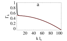
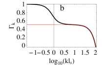
Figure 1: (Color online.) The growth exponent $\Gamma_{k}$ of the clustering mode versus the rescaled wave number $kl_{s}$ (a) and versus $\log\,(kl_{s})$ (b) as predicted from the complete linear stability analysis of a HCS McNamara1 (the thick black line) and from the reduced equation (19) (the thin red line). The physical (not rescaled) units are used, and the parameters are $\gamma=2$ and $k_{cr}l_{s}=100$. At $kl_{s}\lesssim 1$ the isobaric growth rate (19) underestimates the actual growth rate, but in the region of $kl_{s}\gg 1$ excellent agreement between the two results is observed.

Having successfully tested our reduced model in these two simple cases, we now consider nonlinear evolution.

V Neglecting heat diffusion causes a density blowup

As we mentioned earlier, the only governing parameter in Eq. (19), except parameters introduced by the initial condition, is the rescaled system length/mass ${\cal L}$. In the limit of ${\cal L}\gg 1$, and for a sufficiently large-scale initial condition, one can drop the diffusion term in Eq. (19). This approximation is valid as long as the solution remains large-scale. At the level of linear stability analysis this (intermediate-wavelength) approximation is fully justified. Here Eq. (28) becomes $\hat{\Gamma}_{k}\simeq 1$, and one is interested in the nonlinear development of the growing perturbations. With the diffusion term dropped we obtain

$$\frac{\partial w}{\partial\tau}=-1+w\,\left\langle w\right\rangle\,.$$ (31)

This nonlinear integro-differential evolution equation is exactly soluble for any initial data $w(m,0)$. The complete solution is presented below. The main result here is that, for any inhomogeneous initial condition, the solution of Eq. (31) develops a zero $w$ (hence an infinite density) in a finite time. Let us first discuss the properties of the solution in a close vicinity of the singularity $w\to 0$. In the leading order we can neglect the integral term in Eq. (31) and obtain $\partial w/\partial\tau=-1$, so that $w(m,\tau)=\tilde{w}(m)-\tau$, where $\tilde{w}(m)$ is a smooth function. The singularity occurs in the Lagrangian point $m_{0}$ that corresponds to the minimum of $\tilde{w}(m)$. The leading order behavior of the (rescaled) gas density near the singularity is described by the following equation:

$$\rho(m,\tau)=\left[\tau_{c}-\tau+\frac{1}{2}\frac{d^{2}\tilde{w}}{dm^{2}}\left(m_{0}\right)(m-m_{0})^{2}\right]^{-2}\,,$$ (32)

where the time of singularity $\tau_{c}=\tilde{w}(m_{0})$. The singularity structure, as described by Eq. (32), coincides with that exhibited by a family of exact solutions of the full set of ideal hydrodynamic equations [that is, Eqs. (2)-(4) without the viscous and heat diffusion terms], reported in Ref. Fouxon1 ; Fouxon2 . At $\tau=\tau_{c}$ the density blows up as $\rho(m,\tau_{c})\sim(m-m_{0})^{-4}$. Going back to the Eulerian coordinate, we obtain a finite-mass density blowup $\rho(x,\tau_{c})\sim|x-x_{0}|^{-4/5}$, where $x_{0}$ is the Eulerian coordinate of the singularity. We refer the reader to Ref. Fouxon2 for a detailed analysis of the structure of this singularity, as observed in the gas density, temperature and velocity. Notably, the pressure field does not have any singularity in the exact solutions Fouxon1 ; Fouxon2 , and is approximately constant in a narrow region around the density singularity. That is, the density blowup, as featured by the exact solutions of ideal granular hydrodynamics Fouxon1 ; Fouxon2 , locally obeys an isobaric scenario, as was noticed in Ref. Fouxon2 . This provides the reason why the same type of singularity appears in our reduced low Mach number theory.

Now we present a complete solution of Eq. (31). First, we obtain a closed evolution equation for the (necessarily positive) quantity $\chi(\tau)=\left\langle w(m,\tau)\right\rangle$ by integrating the both sides of Eq. (31) over $m$ from $0$ to ${\cal L}$:

$$\frac{d\chi(\tau)}{d\tau}=-1+\chi^{2}\,.$$ (33)

We consider the solution of this equation with the initial condition

$$\chi_{0}=\left\langle w(m,0)\right\rangle=\left\langle\rho(m,0)^{-1/2}\,\right\rangle\leq 1\,.$$

The solution can be written as

$$\chi(\tau)=\frac{\chi_{0}-\tanh(\tau)}{1-\chi_{0}\tanh(\tau)}\,,$$ (34)

Now we can rewrite Eq. (31) as

$$\frac{\partial w}{\partial\tau}-\chi(\tau)\,w(m,\tau)=-1\,,$$ (35)

where $\chi(\tau)$ is given by Eq. (34). Equation (35) is easily soluble:

$$w(m,\tau)=\frac{w(m,0)+\chi_{0}\left[\cosh\left(\tau\right)-1\right]-\sinh\left(\tau\right)}{\cosh\left(\tau\right)-\chi_{0}\sinh\left(\tau\right)}\,.$$ (36)

The presence of the factor $\chi_{0}\left[\cosh\left(\tau\right)-1\right]-\sinh\left(\tau\right)$ in the numerator of Eq. (36) causes, for any (non-constant) initial data $w(m,0)$, a singularity $w\to 0$ in a finite time. The singularity occurs at the Lagrangian point $m_{0}$ where the function $w(m,0)$ has its minimum, at time

$$\tau_{c}=\ln\left[\frac{\Delta w+\left(\Delta w^{2}+1-\chi_{0}^{2}\right)^{1/2}}{1-\chi_{0}}\right]\,$$ (37)

where $\Delta w\equiv w(m_{0},0)-\chi_{0}$. Note that $\Delta w=(1/{\cal L})\int_{0}^{{\cal L}}[w(m_{0},0)-w(m,\tau)]dm\,\leq 0$.

Now we compute the (rescaled) pressure $p(\tau)$ from Eq. (20) [note that the right hand side is simply $\chi(\tau)$ given by Eq. (34)],

$$p(\tau)=\left(\cosh\tau-\chi_{0}\sinh\tau\right)^{2\gamma}\,,$$ (38)

and use this result in Eq. (21) for the rescaled physical time:

$$t=\gamma\int_{0}^{\tau}\frac{d\tau^{\prime}}{\left(\cosh\tau^{\prime}-\chi_{0}\sinh\tau^{\prime}\right)^{\gamma}}\,.$$ (39)

For $\gamma=2$ (a 2D gas of disks) this integral is elementary, and the result is

$$t=\frac{2}{\coth\tau-\chi_{0}}\,.$$ (40)

Now we can express $\tau$ through $t$,

$$\tau=\mbox{arccoth}\left(\frac{2}{t}+\chi_{0}\right)\,$$ (41)

and rewrite Eqs. (36) and (38) (for $\gamma=2$) as

$$w(m,t) = \frac{1}{2}\{\left[w(m,0)-\chi_{0}\right]\sqrt{4+4\chi_{0}t-(1-\chi_{0}^{2})t}$$ (42)

$$+ 2\chi_{0}-(1-\chi_{0}^{2})t\}\,.$$

and

$$p=\left[1+\chi_{0}t-\left(1-\chi_{0}^{2}\right)\frac{t^{2}}{4}\right]^{-2}\,.$$ (43)

So, the solution for $\gamma=2$ is surprisingly simple. We remind that, in view of the chosen rescaling, the initial condition $w(m,0)$ must obey $\left\langle w^{2}(m,0)\right\rangle=1$. To return to the HCS and Haff’s law in Eqs. (42) and (43) one should put there $w(m,0)=\chi_{0}=1$. Equation (43) shows that Haff’s law is an upper bound for the thermal energy loss rate: any deviation from homogeneity brings about $\chi_{0}<1$ and a slower thermal energy decay.

Let us note that the solution (34) for $\chi(\tau)$ vanishes at $\tau_{*}=(1/2)\,\ln[(1+\chi_{0})/(1-\chi_{0})]$ and becomes negative at larger $\tau$. This is in apparent contradiction with the positivity of $w$ that dictates $\chi(\tau)=\left\langle w(m,\tau)\right\rangle\geq 0$. The contradiction is resolved by noting that $\tau_{*}$ is always greater than the singularity time $\tau_{c}$, beyond which the solution does not apply. [To see that $\tau_{c}\leq\tau_{*}$ one can use, in Eq. (37), that $\Delta w+\left(\Delta w^{2}+1-\chi_{0}^{2}\right)^{1/2}\leq\left(1-\chi_{0}^{2}\right)^{1/2}$ for any $\Delta w\leq 0$.] Similarly, the pressure as predicted by Eq. (38) or Eq. (43) would start increasing at some time. At physically meaningful times $\tau<\tau_{c}$, however, we have $\chi(\tau)>0$, and the pressure always decreases in accord with Eq. (20).

As a simple illustration of our solution (36), let us chose the following initial condition: $w(m,0)=\left[1+\delta\cos(2\pi m/{\cal L})\right]^{1/2},\,0<\delta<1$. In this case

$$\chi = \frac{1}{\pi}\left[\sqrt{1-\delta}\;\mbox{E}\left(\frac{2\delta}{\delta-1}\right)+\sqrt{\delta+1}\;\mbox{E}\left(\frac{2\delta}{\delta+1}\right)\right]\,,$$

where $\mbox{E}(\dots)$ is the complete elliptic integral of the second kind, see e.g. Abramowitz . Figure 2a shows, at different times, the rescaled inverse density $1/\rho(m,\tau)$, as obtained from Eq. (36), for $\delta=0.1$ and ${\cal L}=100$. Figure 2b depicts, at the same times, the rescaled Eulerian coordinate $x=\int_{0}^{m}w^{2}(m^{\prime},\tau)dm^{\prime}$ versus the Lagrangian coordinate $m$. Figure 2c shows the rescaled inverse density in the rescaled Eulerian coordinates and illustrates the emergence of the cusp density singularity at $x={\cal L}/2$. The inverse density behaves like $(m-m_{0})^{4}$ at small $m-m_{0}$ in the Lagrangian coordinate, and like $(x-x_{0})^{4/5}$ at small $x-x_{0}$ in the Eulerian coordinate. This simple example is instructive as, for $\delta\ll 1$, this initial condition corresponds to a small single-mode density perturbation, so the initial evolution is describable by the linear theory.

Figure 2: The density history of a freely cooling gas of inelastic hard disks in a 2D channel in the zero-heat-diffusion limit. The rescaled initial density $\rho(m,0)=\left[1+0.1\cos(2\pi m/{\cal L})\right]^{-1}$. The rescaled system length/mass ${\cal L}=100$. Panel a: the rescaled inverse density of the gas, $1/\rho$, versus the Lagrangian mass coordinate $m$ at times $\tau=0$, $1.5$, $2.5$ and the time of singularity $\tau_{c}\simeq 2.8755$. Panel b: the rescaled Eulerian coordinate $x$ versus $m$ at the same times. Panel c: $1/\rho$ versus $x$ at the same times. The sequence of curves is self-explanatory.

VI Heat diffusion arrests the density blowup

A central result of this work is in that, no matter how small initially, the heat diffusion term in Eq. (19) arrests the density blowup. An emerging balance of the inelastic cooling and heat diffusion leads to existence of steady state solutions of Eq. (19). These solutions describe novel cooling states of the granular gas, where the (inhomogeneous) density profile is time-independent, while the (homogeneous) pressure continues to decay with time. We found that, in our rescaled variables, the density profile of the novel cooling state is uniquely defined by the parameter ${\cal L}$. For sufficiently large values of the rescaled length/mass, ${\cal L}\gg 1$, the maximum gas density of the novel cooling state is exponentially large in ${\cal L}$. In the low Mach number theory, considered in this work, the novel cooling states represent global attractors, as they develop for any inhomogeneous initial conditions. Finally, the novel cooling states represent exact solutions of the complete, unreduced set of hydrodynamic equations (2)-(4).

VI.1 Steady state density profiles

Steady-state solutions of Eq. (19) are described by the equation

$$\frac{d^{2}w}{dm^{2}}=w-\left\langle w\right\rangle w^{2}\,.$$ (44)

Notice that, although obtained from our reduced, low Mach number theory, Eq. (44) also follows from the full set of hydrodynamic equations (2)-(4), if one assumes a homogeneous pressure and zero fluid velocity, and transforms to the Lagrangian coordinates.

Equation (44) is defined on the interval $0\leq m\leq{\cal L}$, at the ends of which we demand either periodic, or no-flux (zero first derivative) BCs. The solutions we are interested in must obey the conservation law (22). To get rid of the (a priori unknown) factor $\langle w\rangle$, we introduce a new variable

$$f(m)=\left\langle w\right\rangle w(m)$$ (45)

and obtain

$$\frac{d^{2}f}{dm^{2}}-f+f^{2}=0\,.$$ (46)

Once $f$ is found, one can restore $w$ via

$$w=\frac{f}{\sqrt{\left\langle f\right\rangle}}.$$ (47)

The conservation law (22) enforces a normalization condition

$$\langle f^{2}\rangle=\langle f\rangle\,$$ (48)

that, in virtue of Eq. (46), is obeyed automatically for the periodic or no-flux BCs.

Equation (46) has appeared in numerous applications, and its solutions are well known. It is convenient to interpret $f$ as a coordinate of a Newtonian particle of unit mass, moving in a potential $U(f)=f^{3}/3-f^{2}/2$. The “total energy” $E$ is conserved:

$$E=\frac{1}{2}\left(\frac{df}{dm}\right)^{2}+\frac{f^{3}}{3}-\frac{f^{2}}{2}.$$ (49)

For the bounded (spatially oscillating) solutions, $-1/6\leq E\leq 0$, we can write

$$\frac{f^{3}}{3}-\frac{f^{2}}{2}-E=\frac{(f-a)(f-b)(f-c)}{3},$$ (50)

where $a>b>c$ are the real roots of the cubic polynomial. Then the bounded solutions of Eq. (46) can be written as

$$f(m)=c+(a-c)\,{\mbox{d}n}^{2}\left(\sqrt{\frac{a-c}{6}}m,\,s\right)\,,$$ (51)

where

$$s=\frac{a-b}{a-c}\,,$$ (52)

and ${\mbox{d}n}$ is one of the Jacobi elliptic functions, see e.g. Abramowitz . There are two limits when Eq. (51) simplifies. In the limit of $E=-1/6+\delta E$, $0<\delta E\ll 1$, the solution, $f(m)=1+\sqrt{2\delta E}\cos m$, corresponds to a small-amplitude sinusoidal modulation of the HCS $w(m)=1$. In the limit of $E\to 0$, we have $a=3/2$ and $b=c=0$, so that

$$f(m,E\to 0)=\frac{3}{2}\,{\mbox{d}n}^{2}\left(\frac{m}{2},1\right)=\frac{3}{2}\,\cosh^{-2}\left(\frac{m}{2}\right),$$ (53)

Using Eqs.  (47) and (51), we rewrite the steady state solutions in terms of $w(m)$:

$$w(m)=\frac{c+(a-c)\,{\mbox{d}n}^{2}\left(\sqrt{\frac{a-c}{6}}\,m,s\right)}{\sqrt{c+(a-c)\,\frac{\mbox{E}(s)}{\mbox{K}(s)}}}\,,$$ (54)

where $\mbox{K}(s)$ is the complete elliptic integral of the first kind. The lagrangian spatial period, or wavelength, of the solution (54) is

$$\Pi=\sqrt{\frac{24}{a-c}}\,\mbox{K}(s)\,.$$ (55)

In the limit of $s\to 0$ (or $E\to-1/6$), the wavelength (55) reaches its minimum value $2\pi$. If the rescaled channel length ${\cal L}$ is less than $2\pi$ (for the periodic BCs), or less than $\pi$ (for the no-flux BCs), the only possible steady state is the constant density state $w(m)=1$ corresponding to Haff’s law. This result is in full agreement with the linear stability analysis of Eq. (19), see Eq. (28). When ${\cal L}$ exceeds $2\pi$ (for the periodic BCs), or $\pi$ (for the no-flux BCs), the HCS bifurcates into an inhomogeneous steady state (54). In general, the rescaled channel length/mass ${\cal L}$ must be equal, by virtue of the BCs, to an integer number of $\Pi$ (for the periodic BCs), or to an integer number of $\Pi/2$ (for the no-flux BCs). For sufficiently large value of ${\cal L}$, therefore, a whole family of steady state density profiles exists. Which of the steady state solutions is selected by the dynamics of Eq. (19)?

VI.2 Selected steady-state solutions: the inhomogeneous cooling states

We performed extensive numerical simulations with Eq. (19), using a specially developed numerical scheme described in Appendix A. Both periodic, and no-flux BCs were used. We observed that, when $0<{\cal L}<2\pi$ (for the periodic BCs), or $0<{\cal L}<\pi$ (for the no-flux conditions), the HCS appears, as expected. When ${\cal L}$ exceeds $2\pi$ (for the periodic BCs), a weakly inhomogeneous steady state density profile sets in. As ${\cal L}$ increases further, the weakly inhomogeneous states develops into a strongly inhomogeneous states. The simulations showed that the rescaled length/mass of the gas, ${\cal L}$, uniquely selects the emerging steady state density profile, while the initial $w$-profile does not play any role in the selection. For a given ${\cal L}$ the dynamics always selects, out of the family of steady state solutions (54), the one with the maximum possible wavelength $\Pi$:

$${\cal L}=\left\{\begin{array}[]{ll}\Pi&\mbox{for the periodic BCs}\,,\\ \Pi/2&\mbox{for the no-flux BCs\,.}\end{array}\right.$$ (56)

Snapshots from a typical simulation (one of many that we performed) for the periodic BCs are shown in Fig. 3. The initial condition is this example was

$$w^{2}(m,0) = 1-0.1\,\cos(2\pi m/{\cal L})-0.15\,\sin(2\pi m/{\cal L})$$ (57)

$$+ 0.2\,\cos(4\pi m/{\cal L})-0.05\sin(4\pi m/{\cal L})\,.$$

The rescaled system length/mass ${\cal L}=50$ was sufficiently large to fit in steady state solutions with several oscillations. Nevertheless, the dynamics selected the solution with the spatial period equal to the rescaled system length ${\cal L}$.

Figure 3: Numerical $w$-profiles at times $\tau=0$, $2$, $4$ and $72$, and $1/w$-profile at time $\tau=72$, for ${\cal L}=50$ when starting from the initial condition (57). The two panels for $\tau=72$ also show, by circles, the single hole asymptotes (60) and (61), respectively.

Figures 4 - 6 depict our analytical solutions (54) in the Lagrangian coordinate, and the corresponding density profiles in the Eulerian coordinates, for three different values of the parameter ${\cal L}$. Here we assumed the periodic BCs and (arbitrarily) chose the position of the minimum of $w(m)$ to be in the middle of the channel.

Figure 4: The inhomogeneous cooling state for ${\cal L}=7.025$. Panel a: the Lagrangian steady state solution $w(m)$ as predicted by Eq. (54). Panel b: the rescaled steady state gas density $\rho$ versus the rescaled Eulerian coordinate $x$.

Figure 5: Same as in Fig. 4, but for ${\cal L}=8.886$.

Figure 6: Same as in Fig. 4, but for ${\cal L}=19.869$. Notice the logarithmic scale in panel b.

The maximum (rescaled) gas density versus the rescaled channel length ${\cal L}$, predicted by Eqs. (54) and (55), is shown in Fig. 7. This dependence can serve as a bifurcation diagram of the system. One observes, at ${\cal L}>2\pi$, a supercritical bifurcation from the HCS to an ICS.

Figure 7: The bifurcation diagram of the freely cooling granular gas in a channel. Shown is the maximum (rescaled) steady state density of the gas versus the rescaled channel length ${\cal L}$, predicted by Eqs. (54) and (55). Panel b focuses on a vicinity of the supercritical bifurcation point ${\cal L}=2\pi$.

One can see that, as the parameter ${\cal L}$ increases, the maximum gas density in the cluster grows very fast [note that Fig. 6b shows the density in logarithmic scale]. Let us consider the asymptotic form of the solution at ${\cal L}\gg 1$ in some detail. The density maximum in this case is exponentially large nottoolong . This is due to the behavior of the $s\to 1$ asymptotics of the steady-state solution, see Eq. (53). In this case the “energy” $E$ is very small, and can be expressed through the rescaled system length as $|E|\simeq 72\,\exp(-{\cal L})$. The maximum value of $w(m)$ is

$$w_{max}\simeq\sqrt{\frac{3{\cal L}}{8}}\,.$$ (58)

To obtain the minimum value of $w(m)$ (that corresponds to the maximum value of the density), it is convenient to use the exact relation $w_{min}=b/\sqrt{\langle f\rangle}$ and calculate the asymptotic value of $b$ at $|E|\ll 1$, or ${\cal L}\gg 1$. The result is

$$w_{min}\simeq\sqrt{24{\cal L}}\,e^{-{\cal L}/2}\,,$$ (59)

By virtue of Eq. (53), the asymptotics of the steady state solution (54) at $|m|\ll{\cal L}/2$ is

$$w_{0}(m)\simeq\sqrt{\frac{3{\cal L}}{8}}\,\cosh^{-2}\left(\frac{m}{2}\right)\,,$$ (60)

where, for convenience, we have written the solution on the interval $-{\cal L}/2<m<{\cal L}/2$ and used the approximate equality $\langle f\rangle\simeq 6/{\cal L}$. To calculate the asymptotics of Eq. (54) at $|m|\gg 1$, we can deal directly with Eq. (46) and neglect the $f^{2}$ term. The solution of the resulting elementary equation is a linear combination of $e^{m}$ and $e^{-m}$. The two arbitrary constants can be determined from the two conditions at $|m|={\cal L}/2$: $df/dm=0$ and $w_{0}\equiv f/\sqrt{\langle f\rangle}=w_{min}$, where $w_{min}$ is given by Eq. (59). We obtain

$$w_{0}(m)\simeq\sqrt{24{\cal L}}\,e^{-{\cal L}/2}\cosh({\cal L}/2-|m|)\,,\;\;\;|m|\gg 1\,.$$ (61)

Note that the asymptotes (60) and (61) coincide in their common region $1\ll|m|\ll{\cal L}/2$, where each of them yields

$$w_{0}(m)\simeq\sqrt{6{\cal L}}\,e^{-m}\,.$$ (62)

Note that $\langle w_{0}(m)\rangle\simeq\sqrt{6/{\cal L}}$ is determined by the asymptote (60). We compared the asymptotes (60) and (61) with the numerical solution, shown in Fig. 3, at a late time $\tau=72$. Employing the periodic BCs, we shifted the numerical solution in $m$ so that the maximum of $w(m,\tau=72)$ is at $m=0$. One can see that the agreement is excellent.

As higher $w$ corresponds to a lower gas density, the region of the maximum of $w$ corresponds to a hole in the density. Therefore, we will call the approximate solution, fully determined by Eqs. (60) and (61), the hole solution. The rescaled steady-state gas density, in the limit of ${\cal L}\gg 1$, is

$$\rho(m)\simeq\frac{8}{3{\cal L}}\,\cosh^{4}\left(\frac{m}{2}\right)\,,\;\;\;|m|\ll{\cal L}/2\,,$$ (63)

and

$$\rho(m)\simeq\frac{e^{\cal L}}{24{\cal L}}\,\cosh^{-2}\left(\frac{{\cal L}}{2}-|m|\right)\,,\;\;\;|m|\gg 1\,,$$ (64)

and the maximum and minimum density values are

$$\rho_{max}\simeq\frac{e^{{\cal L}}}{24{\cal L}}\,,\;\;\;\;\;\;\rho_{min}\simeq\frac{8}{3{\cal L}}\,.$$ (65)

Note that Eqs. (58)-(65) work very well already for moderate values of ${\cal L}$. For the dilute hydrodynamics to be still valid in the gas density peak region, we must demand that the peak density be much less than the close packing density. In view of the exponential growth of the maximum density with the parameter ${\cal L}$, see Eq. (65), this leads to a stringent condition:

$$\rho_{0}\sigma^{d}\ll 24{\cal L}\,e^{-{\cal L}}\,.$$

If this condition is not fulfilled, the dilute theory will break down, and the attempted density blowup will be regularized by close-packing effects.

The general form of the steady state density profile in the Eulerian coordinates is quite cumbersome. However, its asymptotic form at ${\cal L}\gg 1$ that corresponds to the Lagrangian profiles (60) and (61) is both elementary and instructive. For Eq. (60) one finds, after some algebra,

$$w_{0}(x)=\sqrt{\frac{3{\cal L}}{2}}\,\cos\left[\frac{1}{3}\arccos\left(1-\frac{8x^{2}}{{\cal L}^{2}}\right)\right]-\sqrt{\frac{3{\cal L}}{8}}\,.$$ (66)

This asymptotics is valid at $e^{-{\cal L}}\ll 1-2|x|/{\cal L}$, that is almost over the whole channel $|x|<{\cal L}/2$ except in a narrow region. This region, however, includes a significant part of the gas mass, as evidenced by the size of this region in the Lagrangian coordinate and by the non-integrable diverging power-law asymptotics of the gas density:

$$\rho(x)\simeq\frac{1}{{\cal L}-2|x|}\;\;\;\mbox{at}\;\;\;e^{-{\cal L}}\ll 1-\frac{2|x|}{{\cal L}}\ll 1\,.$$ (67)

There is of course no actual density divergence here, as Eq. (67) does not hold close to the end points: at $1-2|x|/{\cal L}\lesssim e^{-{\cal L}}$. To find the density profile in this exponentially narrow region, we express the relation between $x$ and $m$ as

$$x = \int_{0}^{m}w_{0}^{2}(m^{\prime})\,dm^{\prime}$$ (68)

$$= \int_{0}^{{\cal L}/2}w_{0}^{2}(m^{\prime})\,dm^{\prime}-\int_{m}^{{\cal L}/2}w_{0}^{2}(m^{\prime})\,dm^{\prime}$$

$$= {\cal L}/2-\int_{m}^{{\cal L}/2}w_{0}^{2}(m^{\prime})\,dm^{\prime}\,.$$

This form is convenient in the vicinity of $m={\cal L}/2$. The case of $m=-{\cal L}/2$ can be treated similarly, and the expressions that follow are valid in both cases. For $|m|\gg 1$ Eqs. (68) and (61) yield

$$|x|\simeq\frac{{\cal L}}{2}-6\,{\cal L}e^{-{\cal L}}\left[{\cal L}-2|m|+\sinh({\cal L}-2|m|)\right]\,.$$ (69)

Equations (64) and (69) determine, in a parametric form and in elementary functions, the density profile in the region sufficiently far from the density minimum. Still simpler results can be obtained in the following two sub-regions. The first is the common region ${\cal L}/2-|m|\gg 1$ but $|m|\gg 1$. The asymptotics of Eqs. (64) and (69) at ${\cal L}/2-|m|\gg 1$ become $\rho=e^{2|m|}/(6{\cal L})$, and $|x|\simeq{\cal L}/2-3{\cal L}e^{-2|m|}$, therefore $\rho=({\cal L}-2|x|)^{-1}$ which coincides with the asymptotics (67) of Eq. (66). The second limit corresponds to ${\cal L}/2-|m|\ll 1$. Here Eq. (64) becomes

$$\rho(m)\simeq\frac{e^{{\cal L}}}{24{\cal L}}\left[1-\left(\frac{{\cal L}}{2}-|m|\right)^{2}\right]\,,$$

whereas Eq. (69) yields $|x|={\cal L}/2-24{\cal L}e^{-{\cal L}}({\cal L}/2-|m|)$. The resulting Eulerian density profile is

$$\rho(x)\simeq\frac{e^{{\cal L}}}{24{\cal L}}\left[1-\left(\frac{e^{{\cal L}}}{24{\cal L}}\right)^{2}\left(\frac{{\cal L}}{2}-|x|\right)^{2}\right]\,.$$ (70)

VI.3 Energy decay for the ICSs

Now let us consider the evolution of the (rescaled) total energy of the gas,

$$E_{tot}(t)=\int_{0}^{{\cal L}}\left(\frac{p}{\gamma-1}+\frac{\rho v^{2}}{2}\right)dx\,,$$ (71)

where the first term under the integral is the thermal energy density, and the second term is the macroscopic kinetic energy density. For the low Mach number flow, that we are dealing with in this work, the first term is almost independent of $x$, while the second term is negligible. As a result, the energy decays, in the leading order, in the same way as the pressure. The pressure decay $p(\tau)$ is described by Eq. (20), whereas to go back to the physical time we use Eq. (21). For our steady state solutions we arrive at a generalized Haff’s law

$$p(t)=\frac{1}{(1+\langle w\rangle t)^{2}}.$$ (72)

As $\langle w\rangle\leq\langle w^{2}\rangle^{1/2}=1$, the energy decay for the ICS is always slower than for the HCS, see Eq. (25). A more explicit form of the generalized Haff’s law (72) is

$$p(t)=\left[1+t\sqrt{c+(a-c)\,\frac{\mbox{E}(s)}{\mbox{K}(s)}}\right]^{-2}.$$ (73)

Now we consider the particular case of the single hole solution $w_{0}(m)$. As $\langle w_{0}(m)\rangle\simeq\sqrt{6/{\cal L}}$, we obtain for the pressure (in the physical units)

$$p(\tau)=p_{0}\exp\left(-2\sqrt{6}\gamma{\cal L}^{-1/2}\tau\right)\,.$$ (74)

Using Eq. (21), we find the original (physical) time $t$ in terms of $\tau$ (again, in the physical units):

$$t=\frac{(6{\cal L})^{1/2}}{3\Lambda\rho_{0}^{1/2}p_{0}^{1/2}}\left(e^{\sqrt{6}\gamma{\cal L}^{-1/2}\tau}-1\right)\,.$$ (75)

This yields a generalized Haff’s law

$$p(t)=\frac{p_{0}}{\left(1+t/\tilde{t}_{c}\right)^{2}}$$ (76)

with a characteristic cooling time

$$\tilde{t}_{c}=\frac{(6{\cal L})^{1/2}}{3\Lambda\rho_{0}^{1/2}p_{0}^{1/2}}\,.$$ (77)

As ${\cal L}\gg 1$, the cooling time $\tilde{t}_{c}$ is much longer than the cooling time $t_{c}$ corresponding to the HCS:

$$\frac{t_{c}}{\tilde{t}_{c}}=\left(\frac{6}{{\cal L}}\right)^{1/2}\ll 1.$$ (78)

VI.4 Relaxation to the single hole state

Here we study the late-time dynamics of relaxation of the cooling gas towards the single hole state: the cooling state observed for ${\cal L}\gg 1$, that is, for $l_{cr}\ll L\ll l_{s}$. We put $w(m,\tau)=w_{0}(m)+w_{1}(m,\tau)$, where $w_{0}(m)$ is the single hole asymptotics (60), and linearize Eq. (19) with respect to the small correction $w_{1}$. We obtain

$$w_{0}\frac{\partial w_{1}}{\partial\tau}=\left(2w_{0}\left\langle w_{0}\right\rangle-1\right)w_{1}+\left\langle w_{1}\right\rangle w_{0}^{2}+\frac{\partial^{2}w_{1}}{\partial m^{2}}\,.$$ (79)

In the language of the linear stability analysis, the conservation law (22) becomes $\left\langle w_{0}(m)w_{1}(m,\tau)\right\rangle=0$. Integrating Eq. (79) over the box, one can see that, once this condition holds at $\tau=0$, it continues to hold at $\tau>0$.

As will become clear shortly, a natural complete set of eigenfunctions for the linear equation (79) is provided by the following eigenvalue problem:

$$y_{n}^{\prime\prime}(m)+\left[-1+\lambda_{n}w_{0}(m)\right]y_{n}(m)=0\,.$$ (80)

for the eigenfunctions $y_{n}(m)$ obeying the BCs $y_{n}(\pm\infty)=0$. (Here we have moved the boundaries to infinity which is accurate with an exponential accuracy in the large parameter ${\cal L}\gg 1$.) Equation (80) can be viewed as a stationary Shrödinger equation (with $\hbar=1$) for a particle with mass $1/2$ and a fixed energy $-1$ in the Pöschl-Teller potential well, see e.g. Ref. LLQM . The depth of the well is determined by the eigenvalues $\lambda_{n}$. The spectrum of this problem is discrete:

$$\lambda_{n}=\frac{(n+2)(n+3)}{(6{\cal L})^{1/2}}\,,\;\;\;\;\;n=0,1,2,3,\dots\,.$$ (81)

For even values of $n$ one obtains even eigenfunctions:

$$y_{n}^{even}(m) = A_{n}\cosh^{2n+3}\left(\frac{m}{2}\right)$$ (82)

$$\times {}_{2}F_{1}\left[n+\frac{1}{2},n+\frac{5}{2};\frac{1}{2};-\sinh^{2}\left(\frac{m}{2}\right)\right],$$

whereas for odd values of $n$ one obtains odd eigenfunctions:

$$y_{n}^{odd}(m) = B_{n}\cosh^{2n+4}\left(\frac{m}{2}\right)\sinh\left(\frac{m}{2}\right)$$ (83)

$$\times {}_{2}F_{1}\left[n+\frac{3}{2},n+\frac{7}{2};\frac{3}{2};-\sinh^{2}\left(\frac{m}{2}\right)\right].$$

Here ${}_{2}F_{1}(\dots)$ is the hypergeometric function, and $A_{n}$ and $B_{n}$ are constants that we fix using the orthonormality conditions

$$\int_{-\infty}^{+\infty}y_{k}(m)y_{n}(m)w_{0}(m)\,dm=\delta_{kn}\,,$$ (84)

the Kroneker delta. The fundamental mode $y_{0}(m)$ is even, it is proportional to $w_{0}(m)$:

$$y_{0}(m)=C_{0}\,w_{0}(m)=(75/2{\cal L})^{1/4}\,\cosh^{-2}(m/2)\,,$$

where $C_{0}=5^{1/2}6^{-1/4}{\cal L}^{-3/4}$. The next mode is the first odd eigenfunction $y_{1}(m)$, proportional to $dw_{0}(m)/dm$:

$$y_{1}(m)=-\frac{3^{1/4}\sqrt{35}\cosh^{-2}\left(m/2\right)\tanh\left(m/2\right)}{2^{7/4}{\cal L}^{1/4}}\,.$$

The next one is the second even eigenfunction

$$y_{2}(m)=-\frac{3^{3/4}\sqrt{5}\,(3\cosh m-4)\cosh^{-4}(m/2)}{2^{7/4}{\cal L}^{1/4}}\,,$$

and so on. Let us expand $w_{1}(m,\tau)$ in this complete set of eigenfunctions:

$$w_{1}(m,\tau)=\sum_{n=0}^{\infty}a_{n}(\tau)\,y_{n}(m)\,,$$

substitute this expansion in Eq. (79), multiply the resulting equation by $y_{k}(m)$, $k=0,1,2,\dots$ and integrate over $m$ from $-\infty$ to $\infty$. Using Eq. (80), we arrive at the following equations for the time-dependent amplitudes $a_{k}(\tau)$:

$$\frac{da_{k}(\tau)}{d\tau}=-\Gamma_{k}a_{k}(\tau)\;\;\;\mbox{for}\;k\neq 0\,,$$ (85)

and

$$\frac{da_{0}(\tau)}{d\tau}=2\left\langle w_{0}\right\rangle\,a_{0}(\tau)+\frac{1}{C_{0}}\sum_{n=1}^{\infty}a_{2n}(\tau)\left\langle y_{2n}\right\rangle\,.$$ (86)

Here

$$\Gamma_{k}=\lambda_{k}-2\left\langle w_{0}\right\rangle=\frac{(k-1)(k+6)}{(6{\cal L})^{1/2}}\,,\;\;\;k=1,2,\dots\,,$$ (87)

and we have used the equality $\lambda_{0}=\langle w_{0}\rangle$. The amplitude equations (85) and (86), together with the initial conditions $a_{k}(0)$, $k=0,1,2,\dots$, enable us to solve the initial value problem for the evolution of the small perturbation $w_{1}(m,\tau)$. Equations (85) show that each of the odd and even modes $k=1,2,3,\dots$ evolve independently of other modes: the $k=1$ mode has a zero decay rate (which is expected, as it is a translational mode), while the higher modes decay exponentially in time $\tau$ :

$$a_{k}(\tau)=a_{k}(0)\exp(-\Gamma_{k}\tau)\,,\;\;\;k=1,2,3,\dots.$$ (88)

The $k=0$ mode behaves quite differently from other modes, as it is affected by the rest of the even modes of the system, see Eq. (86). The solution of Eq. (86) is:

$$a_{0}(\tau) = \left[a_{0}(0)+\frac{1}{C_{0}}\sum_{n=1}^{\infty}\frac{a_{2n}(0)\left\langle y_{2n}\right\rangle}{\lambda_{2n}}\right]\,\exp\left(2\left\langle w_{0}\right\rangle\tau\right)$$ (89)

$$- \frac{1}{C_{0}}\sum_{n=1}^{\infty}\frac{a_{2n}(0)\left\langle y_{2n}\right\rangle}{\lambda_{2n}}\,\exp\left(-\Gamma_{2n}\tau\right)\,.$$

Now we prove that the term in the square brackets vanishes. At $\tau=0$ the conservation law (22) can be written as

$$\left\langle w_{0}(m)\,\sum_{n=0}^{\infty}a_{2n}(0)y_{2n}(m)\right\rangle=0,$$

which yields

$$a_{0}(0)+\frac{1}{C_{0}}\sum_{n=0}^{\infty}a_{2n}(0)\left\langle w_{0}y_{2n}\right\rangle=0\,.$$ (90)

By virtue of the identity $\left\langle y_{2n}\right\rangle=\lambda_{2n}\left\langle w_{0}y_{2n}\right\rangle$ [which readily follows from Eq. (80)], the left side of Eq. (90) coincides with the term in the square brackets in Eq. (89). Therefore, the final result for $a_{0}(\tau)$ is

$$a_{0}(\tau)=-\frac{1}{C_{0}}\sum_{n=1}^{\infty}\frac{a_{2n}(0)\left\langle y_{2n}\right\rangle}{\lambda_{2n}}\,\exp\left(-\Gamma_{2n}\tau\right)\,.$$ (91)

$a_{0}(\tau)$ can behave non-monotonically at short times. However, it always decays at long times, and the dominant decay rate, at $\tau\gg{\cal L}^{1/2}$, is $\Gamma_{2}$.

Figure 8: The difference $w_{1}(m,\tau)$ between the time-dependent solution and the single-hole steady state asymptotics (60) at different (late) times for the simulation shown in Fig. 3.

Figure 9: Testing the linear stability analysis of the single hole solution. The circles show, in the logarithmic scale, $\mbox{max}_{m}\,|w_{1}(m,\tau)|$ (see Fig. 8) versus time $\tau$. The solid line depicts our theoretical prediction for long times, when the relaxation is dominated by the mode $y_{2}$, so that $\mbox{max}_{m}\,|w_{1}|=c_{0}\exp(-\Gamma_{2}\tau)$, where $\Gamma_{2}=8/\sqrt{6{\cal L}}\simeq 0.462$. The adjustable parameter $c_{0}=33.5$.

Figures 8 and 9 present a comparison of the linear stability analysis with the simulation shown in Fig. 3. Figure 8 shows, at late times, the deviation of the numerical solution from the theoretical single-hole steady state asymptotics (60) for the simulation shown in Fig. 3. As time proceeds, the deviation tends to zero as expected. Figure 9 compares the numerically observed decay rate of the deviation with the analytical result (87) for the decay rate $\Gamma_{2}$ that dominates at late times, and very good agreement is observed.

Using Eqs. (75) and (87), we can see that the exponential decay in $\tau$ of each of the eigenmodes $k=1,2,\dots$, see Eq. (88), becomes a power-law decay in the physical time:

$$a_{k}(t)=a_{k}(0)\left(1+\frac{t}{\tilde{t}_{c}}\right)^{-\frac{(k-1)(k+6)}{6\gamma}}\,,\;\;\;k=1,2,\dots\,,$$

with $\tilde{t}_{c}$ from Eq. (77). The zero mode dynamics (91) can be represented as a superposition of terms, each of which decaying as a power law in the physical time. Therefore, the mismatch $w(m,t)-w_{0}(m)$ between the time-dependent solution $w(m,t)$ and the single hole solution $w_{0}(m)$ decays, at long times, as $\sim(t/\tilde{t}_{c})^{-4/(3\gamma)}$.

Before concluding this section we note that the $k=1$ mode turned out to be marginally stable because we neglected corrections exponentially small with respect to the rescaled system length ${\cal L}$. In a more accurate treatment this mode would cease to be a translational mode and acquire a non-zero (although exponentially small) damping rate in time $\tau$. This would lead to a power law decay of this mode in time $t$ with a power exponent that is exponentially small in ${\cal L}$.

VII Coarsening dynamics and statistics of holes

Numerical simulations with Eq. (19) show that, for a sufficiently large rescaled length/mass of the system, ${\cal L}\gg 1$, many peaks of $w$ (hence, holes of the gas density) nucleate in the system nottoolong . The nucleation stage, as observed numerically, is shown in the upper left panel of Fig. 10. The initial condition $w(m,\tau=0)$ simulated white noise, as we chose $w^{2}(m,\tau=0)$ to be equal to $1$ plus a sum of a very large number of Fourier harmonics with (very small) random amplitudes drawn from a uniform distribution. As evidenced by Fig. 10, the further evolution of the holes resembles Ostwald ripening Ostwald . At this stage nucleation of new holes does not occur anymore, and a competition between the holes begins. Underdense holes release their material into the environment and become more pronounced (even less dense), while holes with more material continue to suck the material in until they disappear. At some stage the holes which gas density previously decreased, reverse the trend and begin to densify. At the end of this coarsening process only one hole (that was the least dense in the beginning) remains and forms the single-hole solution (60) and (61) switch . Clearly, the holes compete non-locally: via the spatial averaging term of Eq. (19).

Figure 10: Nucleation and coarsening of holes when starting from a small amplitude “white noise” density perturbation around $w=1$. Shown is a small fragment of the system of rescaled length/mass ${\cal L}=10^{6}$ at indicated times.

Can one build upon the analogy with Ostwald ripening and develop an asymptotic theory of the hole coarsening dynamics? Consider a late stage of the dynamics when there are $N$ holes, located sufficiently far from each other, and centered at points $m_{i}$, $i=1,2,\dots,N$. A simple theory assumes that the spatial shape of each hole coincides with that of the limiting steady state asymptotics (60), but with its own amplitude $A_{i}(t)$ that depends on time. The latter assumption is based on a remarkable fact that, up to exponentially small corrections, Eq. (19) admits the following ansatz:

$$w(m,\tau)=\sum_{i=1}^{N}A_{i}(\tau)\,\cosh^{-2}\left(\frac{m-m_{i}}{2}\right)\,.$$ (92)

Plugging it into Eq. (19) and neglecting exponentially small overlap terms, we find that the equation is satisfied once the following $N$ relations hold:

$$\dot{A}_{i}(\tau)=S(\tau)A_{i}(\tau)-\frac{3}{2}\,,\;\;\;\;\;\;i=1,2,\dots,N\,.$$ (93)

Here

$$S(\tau)=\frac{4}{{\cal L}}\,\sum_{i=1}^{N}A_{i}(\tau)\simeq\left\langle w(m,\tau)\right\rangle\,.$$ (94)

Once all the initial amplitudes $A_{i}(0)$ of the holes are known, the effective dynamical system (93) provides a complete description of the problem. The conservation law (22) of the original Eq. (19) becomes an integral of motion of the dynamical system (93):

$$\sum_{i=1}^{N}A_{i}^{2}(\tau)=\frac{3{\cal L}}{8}=const\,.$$ (95)

Equations (93)-(95) are similar to (the discrete version of) the Lifshitz-Slyozov theory of Ostwald ripening LS , and their properties give a qualitative explanation to the properties of coarsening observed in Fig. 10. Indeed, the holes with amplitudes greater than the (time-dependent) critical amplitude $A_{cr}(\tau)=(3/2)S^{-1}(\tau)$ grow in the amplitude, while holes with amplitudes less than $A_{cr}(\tau)$ decrease their amplitude and disappear. As $A_{cr}(\tau)$ grows with time, the holes that previously grew in the amplitude begin to decrease their amplitude and finally disappear.

A natural further step is to assume $N\gg 1$, treat the hole amplitude as a continuous variable and deal with the probability distribution $F(A,\tau)$ of the hole amplitudes $A$ at time $\tau$. The corresponding theory can be formulated in the spirit of the Lifshitz-Slyozov theory of Ostwald ripening, and we present it in Appendix B. How does this theory compare with numerical simulations? Figure 11 presents some quantitative characterization of the hole coarsening dynamics for the numerical simulation shown in Fig. 10. Shown are the time histories of $\langle w\rangle$ (panel a), of the total number of holes in the system $N$ (panel b) and of the sum of the hole amplitudes squared (panel c) for the simulation shown in Fig. 10. [Because of the noisy initial condition, it takes some time for well-defined holes to nucleate. We started the hole count at the time when the total number of the local maxima of $w(m)$ became equal, for the first time, to the total number of $m$-intervals where $w$ was less than a prescribed small threshold $10^{-4}$.] One can immediately see on the lower panel of Fig. 11 that the conservation law (95) is not obeyed in this simulation. It is not surprising, therefore, that other quantitative predictions of our Lifshitz-Slyozov-type theory, see Appendix B, are also not supported by this simulation. Most directly, the shape of an individual hole does not agree with that assumed in the ansatz (92). The holes observed in this “generic” simulation have a more complicated structure, and are not characterizable by a single parameter such as $A_{i}(\tau)$.

Figure 11: The time histories of $\langle w\rangle$ (a), the number of holes $N$ (b) and the sum of the hole amplitudes squared (c) for the “generic” simulation (starting from a small amplitude noise) shown in Fig. 10.

Figure 12: Coarsening of holes when starting from the ansatz (92) with $N_{0}=2\times 10^{4}$ holes. The initial hole amplitudes $A_{i}$ are randomly distributed according to a (positive) half-gaussian with variance 1. This distribution is normalized by the condition $\sum_{i=1}^{N_{0}}A_{i}^{2}=3{\cal L}/8$. Shown is a small fragment of the system of rescaled length/mass ${\cal L}=10^{6}$.

Figure 13: The time histories of $\langle w\rangle$ (a), the number of holes $N$ (b) and the sum of the hole amplitudes squared (c) for the simulation that started from the ansatz (92) and is shown in Fig. 12. Theoretical prediction (95) for $\sum A_{i}^{2}$ is $3{\cal L}/8=375,000$ which agrees with the simulation within a 1% error.

Figure 14: A comparison of the time histories of $\langle w\rangle$ and $N$ from Fig.  13 with theoretical predictions. The solid line in panel a shows the numerical results for $1/\langle w\rangle$ versus time $\tau$. The dashed line shows our theoretical prediction for late times: $\langle w\rangle=1/(\tau-\tau_{f})$, where $\tau_{f}$ is an adjustable parameter (in this simulation $\tau_{f}\simeq 23.9$). Plotted in panel b is the numerical result for $N^{-1/2}$ versus $\tau$ (the solid line), and the theoretical prediction $N^{-1/2}(\tau)=\sqrt{3/{\cal L}}\,(\tau-\tau_{f})$ with no additional adjustable parameters (the dashed line). Here $\sqrt{3/{\cal L}}\simeq 1.73\times 10^{-3}$. The noise, evident in panel b at late times, is due to a small number of holes at those times.

It is therefore remarkable, that the ansatz (92) does describe a stable regime of coarsening. That is, if one starts the simulation, at $\tau=0$, with an ensemble of holes with different amplitudes, describable by the ansatz (92), the ansatz continues to hold and, moreover, the system approaches the simple scaling regime predicted by our theory of Lifshitz-Slyozov type. The results of one such simulation are presented in Figs. 12 - 14. Here the holes were placed at a (sufficiently large) equal distance from each other, and the initial hole amplitudes $A_{i}$ were chosen randomly from a positive half-gaussian with variance 1. One can see a hole coarsening process in Fig. 12: holes with a larger amplitude (that is, with less gas) grow (that is, loose gas) at the expense of holes with a smaller amplitude. The time histories of $\langle w\rangle$ and the number of holes $N$, presented in Fig. 13, resemble those for the previously described “generic” simulation. The behavior of the sum $\sum_{1}^{N}A_{i}^{2}$ is, however, dramatically different: here the conservation law (95) is obeyed with a $1$ percent accuracy. A closer inspection of the time histories of $\langle w\rangle$ and $N(\tau)$ (see Fig. 14) shows that, at late times, these quantities agree with the theoretical predictions from Eqs. (B5) (with $\mu_{1}=1$) and (B10), presented in Appendix B. Indeed, by using only one adjustable parameter: the time shift $\tau_{f}$, related to the time of approaching the scaling regime, we obtained good agreement for the two different quantities. We also checked (not shown) that, at different times, the shapes of individual holes are very well described by the $\cosh^{-2}$ profile assumed in the ansatz (92).

VIII Summary and Discussion

We have developed a nonlinear theory of low Mach number channel flows of freely cooling dilute granular gases with nearly elastic particle collisions. We focused on the case when the sound travel time through the system is much shorter than the cooling time and the heat diffusion time. Then, after a brief transient, the gas pressure becomes (almost) uniform in space. This makes it possible to reduce the granular hydrodynamic equations, in Lagrangian coordinates, to a single nonlinear and nonlocal equation of a reaction-diffusion type. With heat diffusion neglected, the reduced equation becomes integrable, and any inhomogeneous initial condition produces a finite-time density blowup. The density blowup has the same universal features at singularity as those exhibited by a family of exact solutions of the full set of ideal hydrodynamic equations Fouxon1 ; Fouxon2 . The density blowup, however, is arrested by the heat diffusion. As a result a novel, inhomogeneous cooling state (ICS) of the gas emerges which has a time-independent density profile. For channels of an intermediate length that we considered, the ICS represents a global attractor of the system. Both its structure, and the late-time relaxation towards it are determined by a single dimensionless parameter ${\cal L}$ which is of the order of the ratio of the channel length to the critical length predicted by the linear theory of instability of the homogeneous cooling state. The energy decay of the ICS differs considerably from Haff’s law: the characteristic decay time diverges with the size of the system as ${\cal L}^{1/2}$, see Eq. (78). At large ${\cal L}$, the maximum density of the ICS grows exponentially with ${\cal L}$. Therefore, for sufficiently long channels (the rest of parameters being fixed), the dilute gas assumption breaks down, and close packed regions emerge.

For ${\cal L}\gg 1$ the cooling dynamics proceeds as a competition between “holes”. This competition is quite similar to Ostwald ripening. In the simple case when the initial state consists of $N$ well separated holes $\sim\cosh^{-2}(m/2)$, the analogy with Ostwald ripening becomes complete, as the “hole ripening” statistics exhibits a simple dynamic scaling behavior and is describable by a variant of the Lifshitz-Slyozov theory. Here, in analogy with other phase ordering systems with a conserved order parameter, the probability distribution of the holes with respect to their amplitudes approaches, at long times, the special (limiting) self-similar solution, that is analytic at the edge of its (compact) support. However, for a generic, noisy initial condition, the competing holes have a more complicated structure than that described by the ansatz (92). This brings about a lack of simple dynamic scaling. A theory of this regime has yet to be developed.

In the light of the above results, a non-linear development of the clustering instability of the HCS, for intermediate channel lengths, is but a particular case of our low Mach number theory. Ultimately, the instability transforms an (almost) homogeneous initial gas density profile into an inhomogeneous but time-independent density profile: the ICS described above. For ${\cal L}\gg 1$ this transformation occurs through an intermediate state with many holes (and many clusters).

It would be interesting to investigate the ICSs, and relaxation toward them, in MD simulations. To directly test our low Mach number theory, one should choose the MD simulation parameters so as to guarantee the length scale separation $l_{cr}<L\ll l_{s}$ assumed here. We stress that this hierarchy of length scales demands nearly elastic particle collisions: $\sqrt{1-r^{2}}\ll 1$. In addition, the channel length $L$ should not be too large so that the theoretically predicted maximum gas density in the ICs is still small compared to the close packing density of spheres.

It is worth noticing that, in all asymptotic cooling regimes of an inhomogeneous gas that we have investigated, the energy decays slower than in the case of a HCS. Haff’s cooling law, therefore, provides an upper bound on the energy decay rate. In fact, this is a general theorem, universally valid for a low Mach number flow. Indeed, according to Eq. (12), the logarithmic derivative of the pressure (and, therefore, of the total energy) is proportional to $-\langle w\rangle$. For a HCS $\langle w\rangle=1$, whereas for any ICS $\langle w\rangle<1$, by virtue of the Cauchy-Schwarz inequality and the identity $\langle w^{2}\rangle=1$.

What can be said about the opposite, long-wavelength limit, $\lambda\gg l_{s}$, where $\lambda$ is the characteristic length scale of the initial perturbations? Although there has been some progress in this case ELM ; MP ; Fouxon1 , a complete understanding of the dynamics and structure of the flow is still lacking. It should be possible to derive a different reduced model in that limit, and see whether the popular “pressure instability scenario” Goldhirsch is at work there. (It is clear that the pressure instability scenario is irrelevant in the intermediate wavelength limit, considered in the present paper.)

Note that the ICSs, that we have discovered here, are exact solutions of the full set of granular hydrodynamic equations (2)-(4) for a nearly elastic dilute gas, without any reductions. Therefore, a question arises on whether the ICS represents an attractor in the general case, including the long wavelength limit. A complete (unreduced) linear stability analysis around the “hole” asymptotics (60) could be the first step in an attempt to answer this question. Such an analysis can be complemented by numerical hydrodynamic simulations of nonlinear cooling flows, so as to elucidate possible effects of shock waves on the (nonlinear) stability of the ICS.

Does this work, limited to channel flows, have any relevance to the shearing/clustering instability of a freely cooling granular gas in fully multi-dimensional geometries? To begin with, the low Mach number theory can be extended to the higher dimensions, once the characteristic sound travel distance $l_{s}$ is much larger than all system dimensions. This extension should take into a proper account the flow vorticity, in much the same way as it was done in Ref. Glasner where a two-dimensional low Mach number flow of an ideal gas, driven by the heat diffusion, was investigated. Although not very simple, such a reduced description (with the acoustic modes eliminated) will be advantageous compared to the full set of multi-dimensional hydrodynamic equations. Furthermore, the novel ICSs of the granular gas (that represent exact solutions of the unreduced granular hydrodynamic equations) may have multi-dimensional analogs. Finding these analogs, and investigating their stability with respect to multi-dimensional perturbations which have both potential, and solenoidal velocity components, can be a natural next step in developing a more complete nonlinear theory of the shearing/clustering instability. The channel flow theory developed here (see also Refs. ELM ; MP ; Fouxon1 ; Fouxon2 ; Puglisi ) sets the ground for the future work.

Appendix A. Numerical scheme

We employed the following implicit finite difference scheme for a numerical solution of Eq. (19):

$$\frac{w_{i}^{2}-\hat{w}^{2}_{i}}{2\delta\tau}=-w_{i}+w_{i}^{2}\frac{\sum_{i=1}^{n}w_{i}}{n}+Dw_{i}\,,$$ (A1)

where $\delta\tau$ is the time step, $w_{i}=w(m_{i},\tau+\delta\tau)$, $\hat{w}_{i}=w(m_{i},\tau)$. A standard discretization $Dw_{i}$ of the diffusion term was used: for the periodic BCs we put

$$Dw_{i}=\left\{\begin{array}[]{ll}\frac{w_{2}-2w_{1}+w_{n}}{h^{2}}\,,\qquad\quad i=1\,,\\ \frac{w_{i+1}-2w_{i}+w_{i-1}}{h^{2}}\,,\quad 1<i<n\,,\\ \frac{w_{1}-2w_{n}+w_{n-1}}{h^{2}}\,,\qquad i=n\,.\end{array}\right.$$

where $h={\cal L}/n$ is the grid size. The approximation error of this scheme is ${\cal O}(\delta\tau^{2})$ in $\delta\tau$ and ${\cal O}(h^{3})$ in $h$. Note that the scheme conserves exactly the discrete version of the conservation law (22), $\langle w_{i}(\tau)^{2}\rangle=(1/n)\sum_{i=1}^{n}w_{i}^{2}=1$, once $\langle w_{i}(0)^{2}\rangle=1$.

We solved the set of nonlinear algebraic equations (A1) by an iteration procedure based on Newton’s method. To obtain, after linearization, a standard cyclic tridiagonal system, we used the values of $w_{i}$, entering the sum $\sum_{i}^{n}w_{i}$, from the previous iteration. We demanded that the residual (the maximum of the absolute value of the difference between the left and right hand sides of the equations after the iteration process) be less then $10^{-13}$. Because of the finite residual, this procedure conserved the mean square of $w$ with an almost machine precision, but not exactly. Therefore, we enforced an even stricter conservation by adding, at each time step, a constant $c$ to the numerical solution $w_{i}$ found with the iteration procedure. The value of $c$ is determined as follows. We represent the (yet unknown) corrected values $\bar{w}_{i}$ as $\bar{w}_{i}=w_{i}+c$. Then

$$\langle\bar{w}_{i}^{2}\rangle=\frac{1}{n}\sum_{i=1}^{n}\left(w_{i}^{2}+2cw_{i}+c^{2}\right)=\langle w^{2}\rangle+2c\langle w\rangle+c^{2}\,.$$

Now we demand that the right hand side be equal to 1. Neglecting the $c^{2}$ term, we find

$$c=\frac{1-\langle w^{2}\rangle}{2\langle w\rangle}\,.$$

We always obtained $|c|<10^{-14}$ in our computations. This justifies neglecting the $c^{2}$ term.

The typical set of parameters for the investigation of relaxation towards a stationary single hole asymptotics (60) was ${\cal L}=50$ and $n=2.5\times 10^{4}$, so $h=2\times 10^{-3}$. In the hole coarsening simulations we used ${\cal L}=10^{6}$ and $n=2.8\times 10^{6}$, so $h\simeq 0.36$. In all cases the time step was chosen to be $\delta\tau=h^{2}$.

Appendix B. Hole coarsening in the spirit of the Lifshitz-Slyozov theory

Here we treat the hole amplitude (see Section VII) as a continuous variable and deal with the probability distribution $F(A,\tau)$ of the hole amplitudes $A$ at time $\tau$. The total number of holes $N(\tau)=\int_{0}^{\infty}F(A,\tau)\,dA\gg 1$. As there is no nucleation of new holes and no hole mergers, the evolution of $F(A,\tau)$ is described, in the spirit of the Lifshitz-Slyozov theory LS , by a continuity equation in the space of hole amplitudes:

$$\frac{\partial F}{\partial\tau}+\frac{\partial}{\partial A}\left[\left(SA-\frac{3}{2}\right)F\right]=0\,,$$ (B1)

where

$$S(\tau)=\frac{4}{{\cal L}}\,\int_{0}^{\infty}AF(A,\tau)dA\,,$$ (B2)

and

$$\int_{0}^{\infty}A^{2}F(A,\tau)dA=\frac{3{\cal L}}{8}=const\,.$$ (B3)

Equations similar to Eqs. (B1)-(B3) have appeared in the context of the Lifshitz-Slyozov model of Ostwald ripening LS and its analogs for different transport mechanisms AMS2 ; W ; MS ; CP ; GMS . In those systems one is usually interested in the question of whether or not the probability distribution $F(A,\tau)$ approaches, at late times, a self-similar shape. A simple power counting in Eqs. (B1)-(B3) yields

$$F(A,\tau)=\frac{{\cal L}}{4\,\tau^{3}}\,\Phi\left(\frac{A}{\tau}\right)\,,$$ (B4)

where $\Phi(\eta)\geq 0$ is the (yet unknown) rescaled distribution, and the coefficient ${\cal L}/4$ is chosen for convenience. Using Eqs. (B2) and (B3), we obtain

$$S(\tau)=\frac{\mu_{1}}{\tau}\;\;\;\;\;\mbox{and}\;\;\;\;\;\mu_{2}=\frac{3}{2}\,,$$ (B5)

respectively. Here $\mu_{k}$ is the $k$-th moment of the rescaled distribution: $\mu_{k}=\int_{0}^{\infty}\eta^{k}\Phi(\eta)d\eta$. One can already see that the total number of holes $N(\tau)$ goes down as $\tau^{-2}$, while both the average hole amplitude $\bar{A}(\tau)$ and the critical amplitude $A_{cr}(\tau)$ grow linearly with $\tau$. The pre-factors of these power laws will be determined once $\Phi(\eta)$ is found. Plugging Eq. (B4) and the first of Eqs. (B5) into Eq. (B1) we obtain an ordinary differential equation for $\Phi(\eta)$:

$$\left[(\mu_{1}-1)\,\eta-\frac{3}{2}\right]\frac{d\Phi}{d\eta}+(\mu_{1}-3)\,\Phi=0\,,$$ (B6)

whose solution is elementary. As in other variants of the LS-theory, we obtain here a whole family of shape functions $\Phi_{\mu_{1}}(\eta)$, parameterized by the first moment $\mu_{1}$. The solutions exist, with finite moments, for $1\leq\mu_{1}<\infty$. For $\mu_{1}>1$ the solutions have finite support:

$$\Phi_{\mu_{1}}(\eta)=\left\{\begin{array}[]{ll}B_{\mu_{1}}\,\left[\frac{3}{2}-(\mu_{1}-1)\,\eta\right]^{\frac{3-\mu_{1}}{\mu_{1}-1}}&\mbox{if $0<\eta<\eta_{m}$}\,,\\ 0&\mbox{if $\eta>\eta_{m}$\,,}\end{array}\right.$$ (B7)

where $\eta_{m}=(3/2)(\mu_{1}-1)^{-1}$. The constant $B_{\mu_{1}}$ can be determined from the second of Eqs. (B5) (that plays the role of a normalization condition):

$$B_{\mu_{1}}=2^{\frac{2\mu_{1}}{\mu_{1}-1}}\,3^{-\frac{\mu_{1}+1}{\mu_{1}-1}}\,\mu_{1}(\mu_{1}+1)\,.$$

This yields, for $\mu_{1}>1$,

$$N(\tau)=\frac{{\cal L}\mu_{1}(1+\mu_{1})}{6\,\tau^{2}}, \bar{A}(\tau)=\frac{3\Gamma\left(\frac{2}{\mu_{1}-1}\right)\,\tau}{(\mu_{1}-1)^{2}\Gamma\left(\frac{2\mu_{1}}{\mu_{1}-1}\right)}\,,$$

$$A_{cr}(\tau) = (3\tau)/(2\mu_{1})\,.$$ (B8)

For $1<\mu_{1}<3$, the solutions (B7) vanish at $\eta=\eta_{m}$, whereas for $\mu_{1}>3$ they diverge at $\eta=\eta_{m}$. As all the moments $\mu_{k}$ remain finite, the diverging distributions are legitimate.

Figure 15: Rescaled distributions of the hole amplitudes $\Phi_{\mu_{1}}(\eta)$ for $\mu_{1}=2.5$, $2$, $1.5$, and $1$ (the latter corresponding to the limiting distribution). Smaller $\mu_{1}$ are shown by thicker lines.

For $\mu_{1}=1$ we obtain a limiting solution $\Phi_{1}(\eta)=(16/9)\,\exp(-4\eta/3)$ that has an infinite support $0\leq\eta<\infty$. The self-similar probability distribution (B4) becomes

$$F(A,\tau)=\frac{4{\cal L}}{9\,\tau^{3}}\,\exp\left(-\frac{4A}{3\tau}\right)\,.$$ (B9)

In this case

$$N(\tau)=\frac{{\cal L}}{3\,\tau^{2}},\;\;\bar{A}(\tau)=\frac{3\tau}{4},\;\;\mbox{and}\;\;A_{cr}(\tau)=\frac{3\tau}{2}.$$ (B10)

These expressions also follow from Eqs. (Appendix B. Hole coarsening in the spirit of the Lifshitz-Slyozov theory) in the limit of $\mu_{1}\to 1$.

Figure 15 depict the rescaled distributions $\Phi_{\mu_{1}}(\eta)$ for four values of the parameter $\mu_{1}$. Selection of the “correct” self-similar solution out of the family of solution represents a subtle problem that was resolved only recently. It turns out that the selection is only made by (a certain feature of) the initial condition $F(A,\tau=0)$ AMS2 ; MS ; CP ; GMS ; Pego . If $F(A,\tau=0)$ has compact support, the similarity solution, if any, is selected by the behavior of $F(A,\tau=0)$ near the supremum $A_{max}$ of the support. If $F(A,\tau=0)$ has a power-law asymptote near $A_{max}$, the exponent of this power law selects one of the solutions from the family (B7). If $F(A,\tau=0)$ goes to zero exponentially fast at $A\to A_{max}$ (or if the support of $F(A,\tau=0)$ is infinite), the limiting solution (B9) is selected.

This sensitivity to initial conditions shows a certain lack of robustness of the Lifshitz-Slyozov model and its analogs like our Eqs. (B1)-(B3). As a remedy, one has to account for an additional physics (that may be less universal and more system-dependent). For example, in the context of the interface-controlled Ostwald ripening strong selection is achieved via an account of direct droplet merger events CMPS .

As we show in Section VII, the Lifshitz-Slyozov-type model does not agree with numerical simulations that start from generic initial conditions. However, if one starts the simulation with an assembly of holes, describable by the ansatz (92), the ansatz continues to hold, and the system approaches the simple scaling regime predicted by the Lifshitz-Slyozov-type theory. Therefore, we want to pursue the ansatz (92) a bit further, as it provides an interesting, though non-generic, characterization of the hole coarsening. We assume that the limiting distribution (B9), corresponding to $\mu_{1}=1$, is selected and use Eq. (20) and the relation $S(\tau)=1/\tau$ to find the corresponding scaling behavior of the gas pressure $p(\tau)$. We obtain

$$\frac{1}{p(\tau)}\frac{dp}{d\tau}=-2\gamma S(\tau)=-\frac{2\gamma}{\tau}\,,$$ (B11)

which yields $p(\tau)=p_{0}(\tau_{0}/\tau)^{2\gamma}$, where $\tau_{0}$ is an effective “initial” time, and $p_{0}=p(\tau_{0})$. Using Eq. (21), we find the following relation between the original (physical) time $t$ and the new time $\tau$:

$$t=\frac{2\gamma\,\tau^{\gamma+1}}{(\gamma+1)\Lambda\rho_{0}^{1/2}p_{0}\tau_{0}^{\gamma}}\,.$$

As a result,

$$\frac{p(t)}{p_{0}}=\left[\frac{2\gamma\,\tau_{0}}{(\gamma+1)\Lambda\rho_{0}^{1/2}p_{0}\,t}\right]^{\frac{2\gamma}{\gamma+1}}=\left(\frac{t_{0}}{t}\right)^{\frac{2\gamma}{\gamma+1}}\,,$$

where $t_{0}=t(\tau_{0})$. Now, in the low Mach number regime we have been dealing with throughout this paper, the total energy of the gas decays in (almost) the same way as the pressure, so $E_{tot}(t)\sim t^{-\frac{2\gamma}{\gamma+1}}$. We obtain $E_{tot}(t)\sim t^{-4/3}$ and $E_{tot}(t)\sim t^{-5/4}$ in 2d (disks) and 3d (spheres), respectively. Again, the cooling dynamics proceeds slower than that predicted by Haff’s law (25). We checked that the same conclusion holds for any $\mu_{1}$, that is for all possible self-similar distributions of the hole amplitudes.

References

- (1) N.V. Brilliantov and T. Pöschel, Kinetic Theory of Granular Gases (Oxford University Press, Oxford, 2004).
- (2) I. Goldhirsch, Annu. Rev. Fluid Mech. 35, 267 (2003).
- (3) M. A. Hopkins and M. Y. Louge, Phys. Fluids A 3, 47 (1991).
- (4) I. Goldhirsch and G. Zanetti, Phys. Rev. Lett. 70, 1619 (1993); I. Goldhirsch, M.-L. Tan, and G. Zanetti, J. Sci. Comp. 8, 1 (1993).
- (5) S. McNamara, Phys. Fluids A 5, 3056 (1993).
- (6) S. McNamara and W. R. Young, Phys. Rev. E 53, 5089 (1996).
- (7) R. Brito and M. H. Ernst, Europhys. Lett. 43, 497 (1998).
- (8) J. J. Brey, M. J. Ruiz-Montero, and D. Cubero, Phys. Rev. E 60, 3150 (1999).
- (9) S. Luding and H. J. Herrmann, Chaos 9, 673 (1999).
- (10) T.P.C. van Noije and M.H. Ernst, Phys. Rev. E 61, 1765 (2000).
- (11) X. B. Nie, E. Ben-Naim, and S. Y. Chen, Phys. Rev. Lett. 89, 204301 (2002).
- (12) E. Efrati, E. Livne, and B. Meerson, Phys. Rev. Lett. 94, 088001 (2005).
- (13) B. Meerson and A. Puglisi, Europhys. Lett. 70, 478 (2005).
- (14) V. Garzó, Phys. Rev. E 72, 021106 (2005).
- (15) Y. Bromberg, E. Livne, and B. Meerson, in Granular Gas Dynamics, edited by T. Pöschel and N.V. Brilliantov (Springer, Berlin, 2003), p. 251; cond-mat/0305557.
- (16) D. Volfson, B. Meerson, and L. S. Tsimring, Phys. Rev. E 73, 061305 (2006).
- (17) I. Fouxon, B. Meerson, M. Assaf, and E. Livne, Phys. Rev. E 75, 050301(R) (2007).
- (18) I. Fouxon, B. Meerson, M. Assaf, and E. Livne, Phys. Fluids 19, 093303 (2007).
- (19) G.B. Whitham, Linear and Nonlinear Waves (Wiley, New York, 1974), Chapter 2.
- (20) A. Puglisi, M. Assaf, I. Fouxon, and B. Meerson, Phys. Rev. E (in press).
- (21) A.G. Doroshkevich and Ya. B. Zel’dovich, Zh. Eksp. Teor. Fiz. 80, 801 (1981) [Sov. Phys. - JETP 53, 405 (1981)].
- (22) B. Meerson, Phys. Fluids A 1, 887 (1989).
- (23) B. Meerson, Astrophys. J. 347, 1012 (1989).
- (24) I. Aranson, B. Meerson, and P.V. Sasorov, Phys. Rev. E 47, 4337 (1993).
- (25) I. Aranson, B. Meerson, and P.V. Sasorov, Phys. Rev. E 52, 948 (1995).
- (26) D. Kaganovich, B. Meerson, A. Zigler, C. Cohen, and J. Levin, Phys. Plasmas 3, 632 (1996).
- (27) A. Glasner, E. Livne, and B. Meerson, Phys. Rev. Lett. 78, 2112 (1997).
- (28) B. Meerson, Rev. Mod. Phys. 68, 215 (1996).
- (29) Ya. B. Zel’dovich and Yu. P. Raizer, Physics of Shock Waves and High Temperature Hydrodynamic Phenomena, Vol. 1 (Academic Press, New York, 1966).
- (30) M. Abramowitz, Handbook of Mathematical Functions (National Bureau of Standards, Washington, 1964).
- (31) On the other hand, we assume throughout this paper that the channel is not too long, so that the uniform pressure approximation remains valid. Long channels imply, in the low Mach number theory, the double inequality . In terms of the rescaled length/mass of the system , long channels imply .
- (32) This scenario assumes periodic BCs. For the no-flux BCs one finally obtains one-half of the hole, with the density minimum and maximum at the channel ends.
- (33) L.D. Landau and E.M. Lifshitz, Quantum Mechanics. Non-Relativistic Theory (Pergamon, London, 1965), p. 72.
- (34) W. Ostwald, Z. Phys. Chem., Stoechiom. Verwandtschaftsl. 34, 495 (1900).
- (35) I.M. Lifshitz and V. V. Slyozov, J. Phys. Chem. Solids 19, 35 (1961).
- (36) C. Wagner, Z. Elektrochem. 65, 581 (1961).
- (37) B. Meerson and P.V. Sasorov, Phys. Rev. E 53, 3491 (1996).
- (38) J. Carr and O. Penrose, Physica D 124, 166 (1998).
- (39) B. Giron, B. Meerson, and P.V. Sasorov, Phys. Rev. E 58, 4213 (1998).
- (40) B. Niethammer and R. Pego, J. Stat. Phys. 95, 867 (1999).
- (41) M. Conti, B. Meerson, A. Peleg, and P.V. Sasorov, Phys. Rev. E 65, 046117 (2002).