Transport in Graphene p-n Junctions in Magnetic Field

Abstract

Ballistic transport in graphene p-n junctions in the presence of magnetic field exhibits two distinct regimes: At low fields, transport is partially suppressed by the field. When the field exceeds a certain critical value, the junction is pinched off by the Landau level formation. Transmission and conductance are found in the entire range of fields using Lorentz boost and mapping to the Landau-Zener problem. We show that perfect transmission occurs at a field-dependent collimation angle, indicating that the chiral dynamics of massless Dirac fermions persists at a finite magnetic field. A current switch, utilizing field-tunable collimation angle, is proposed. With a generalization of the developed approach we study transmission through p-n junctions in graphene bilayer.

Graphene p-n junctions, fabricated recently in locally gated samples Huard07 ; Williams07 ; Ozyilmaz07 , provide a new tool to study electron transport. Charge carriers in graphene mimic relativistic Dirac particles with zero mass and linear dispersion relation $\varepsilon=\pm v_{F}|{\bf p}|$ with $v_{F}\approx 10^{8}\,{\rm cm/s}$. Graphene p-n junctions are predicted to exhibit signatures of chiral dynamics of massless Dirac particles: perfect transmission normal to the junction Katsnelson06b ; KatsnelsonSSC and collimation of the transmitted particles Cheianov06 . Ballistic transport in p-n junctions was proposed as a means to realize an electron lens Cheianov07 .

The properties of the p-n-p system studied in Ref. Huard07 could be mainly explained by conduction in the disordered p and n regions, rather than in the p-n junctions. Likewise, the effects in quantizing magnetic fields Williams07 ; Ozyilmaz07 were understood from edge state transport in the p and n regions, with the p-n interface merely providing mode mixing Abanin07 . In neither of the experiments Huard07 ; Williams07 ; Ozyilmaz07 the effects of ballistic transmission Katsnelson06b ; Cheianov06 ; Cheianov07 seemed to stand out.

This is not too surprising, given that direct detection of the effects Katsnelson06b ; KatsnelsonSSC ; Cheianov06 ; Cheianov07 would require an angle-resolved measurement and/or very clean samples. Alternatively, one can ask if the behavior Katsnelson06b ; KatsnelsonSSC ; Cheianov06 ; Cheianov07 can be inferred from the dependence of transport properties on the magnetic field that often provides valuable insights into electron dynamics. It is interesting therefore to better understand the signatures of ballistic transmission in external magnetic field, which is the main purpose of the present work.

We start by noting that the coupling of an electron to external fields reflects relativistic character of charge carriers in graphene with the speed of light $c$ replaced by $v_{F}$. In relativistic electro-magnetic theory the fields ${\bf E}$ and ${\bf B}$ are treated on equal footing, playing the role of each other in a moving reference frame. The dynamics of a relativistic particle in uniform fields depends only on the Lorentz invariants ${\bf E}^{2}-{\bf B}^{2}$, ${\bf E}.{\bf B}$ LL-2 . In particular, the dynamics in crossed fields, ${\bf E}.{\bf B}=0$, can be of two main types, magnetic and electric, depending on the relative strength of the fields $E$ and $B$. In the first case, $B>E$, the particle trajectories are described by cyclotron motion superimposed with a drift perpendicular to ${\bf E}$. In the second case, $E>B$, the trajectories are similar to those in the absence of $B$ field, moving asymptotically parallel to ${\bf E}$ and exhibiting no cyclotron motion.

Quantum transport in these two regimes, magnetic and electric, was discussed a while ago AronovPikus66 ; Weiler67 in the context of interband tunneling in two-band semiconductor systems modeled by the Dirac equation. Naturally, both of these regimes can be realized in graphene p-n junctions. In the magnetic case, realized for $B>(c/v_{F})E$ Lukose07 , electron motion is described by quantized Landau levels with a linear dispersion in the momentum perpendicular to ${\bf E}$, i.e. parallel to the junction. This defines relativistic Quantum Hall edge states MacDonald83 transporting charge along the p-n interface. Cyclotron frequency in this regime as a function of $E$ vanishes at $E=(v_{F}/c)B$, signaling collapse of the Landau levels and Quantum Hall effect Lukose07 .

In the electric regime $B<(c/v_{F})E$, which will be of main interest for us here, electrons can move freely along ${\bf E}$, transporting electric current through the junction. Transmission coefficient, found below as a function of $B$, is shown to vanish at the critical field

$$B=B_{\ast}\equiv(c/v_{F})E.$$ (1)

The effect of increasing magnetic field is therefore to pinch off transport through the junction, and transform it into the edge state transport along the junction in the Quantum Hall state at $B>B_{\ast}$. Similar conclusions for tunneling suppression by transverse magnetic field in 3D junctions modeled by Dirac particles with a finite mass were obtained in Refs.AronovPikus66 ; Weiler67 .

In our approach, we solve the Dirac equation in crossed $E$ and $B$ fields exactly with the help of a Lorentz boost. This allows us to treat the monolayer and bilayer cases on equal footing. We find collimated transmission peaked at an angle $\sin\theta_{B}=B/B_{\ast}$, with unit transmission at the peak, $\theta=\theta_{B}$, as in the absence of magnetic field. The net conductance, found by integrating transmission over angles $\theta$, for a wide junction is given by

$$G(B\leq B_{\ast})=\frac{e^{2}}{2\pi h}\frac{w}{d}\left(1-(B/B_{\ast})^{2}\right)^{3/4},$$ (2)

where $d=(\hbar v_{F}/|eE|)^{1/2}$ and $w$ is the p-n interface length (see Fig.1). The suppression of tunneling (2) precedes formation of edge states at the p-n interface at $B>B_{\ast}$.

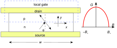
Figure 1: Schematic of a p-n junction in a locally gated sample. For the geometry shown (wide and short sample) the conductance is dominated by the junction. Magnetic field suppresses conductance as $G(B)\propto(1-(B/B_{\ast})^{2})^{3/4}$, Eq.(2).

To estimate the critical field $B_{\ast}$ for the parameter values of Refs.Huard07 ; Williams07 ; Ozyilmaz07 one would have to account for screening of the in-plane field created by gates Fogler07 . To bypass these complications, we assume that a density variation of order $n_{0}\sim 10^{12}\,{\rm cm}^{-2}$ is created in a p-n junction across a distance $\ell\approx 50\,{\rm nm}$. Then the field felt by the electrons is $eE\sim\hbar v_{F}\sqrt{\pi n_{0}}/\ell$, giving

$$B_{\ast}=(c/v_{F})E\sim(\hbar c/e)\sqrt{\pi n_{0}}/\ell.$$ (3)

In terms of the magnetic length $\ell_{B}=\sqrt{\hbar c/eB}$, this translates into $\ell_{B_{\ast}}^{2}=\ell/\sqrt{\pi n_{0}}\approx 260\,{\rm nm}^{2}$, yielding an experimentally convenient value of $B_{\ast}\sim 2.5\,{\rm T}$.

For the p-n junction contribution to dominate over the conduction in the p and n regions, it is beneficial to be in the ballistic regime, similar to Refs.Katsnelson06b ; Cheianov06 ; Cheianov07 , and to use wide and short samples (see Fig.1). These requirements are more relaxed for p-n junctions in epitaxial and bilayer systems, where tunneling is exponentially suppressed owing to the presence of a spectral gap (see below).

We first consider transport in the p-n junction in the absence of magnetic field. Massless Dirac particles in graphene moving near the p-n interface in a uniform in-plane electric field are described by the Hamiltonian

$$H=e\varphi({\bf x})+v_{F}\xi\left(\begin{array}[]{cc}0&p_{+}\\ p_{-}&0\end{array}\right),\quad p_{\pm}=p_{1}\pm ip_{2},$$ (4)

where $\varphi$ is the electrostatic potential used to create the junction, and $\xi=\pm 1$ for the points $K$ and $K^{\prime}$. We consider a p-n interface parallel to the $x$ axis (Fig.1), with the external field ${\bf E}\parallel\hat{y}$ described by $\varphi({\bf x})=-Ex_{2}$.

The eigenstates of (4) are characterized by the momentum component parallel to the junction, $\psi(t,{\bf x})=e^{-i\varepsilon t+ip_{1}x_{1}}\psi(x_{2})$, giving a 1D problem for $\psi(x_{2})$. Following Ref.KaneBlount , we choose to write this problem in momentum representation

$$-ieE\,d\psi/dp_{2}=\tilde{H}\psi,\quad\tilde{H}=v_{F}(p_{1}\sigma_{1}-p_{2}\sigma_{2})-\varepsilon.$$ (5)

As noted in Ref.KaneBlount , momentum representation provides direct access to the asymptotic scattering states, and is thus more beneficial than the position representation.

Indeed, Eq.(5), interpreted as a time-dependent evolution with the Hamiltonian $\tilde{H}$, “time” $p_{2}$, and “Planck’s constant” $eE$, can be identified with the Landau-Zener problem for a two-level system evolving through an avoided crossing. Hence the probability to be transmitted (reflected) in the Dirac problem translates into the probability of a diabatic (adiabatic) Landau-Zener transition. The transmission coefficient can thus be found using the answer for the latter LL-3 , giving

$$T(p_{1})=\exp(-\pi\hbar v_{F}p_{1}^{2}/|eE|),$$ (6)

which agrees with the results of  KaneBlount ; Cheianov06 (see also Andreev07 ).

Alternatively, the result (6) can be put in the context of Klein tunneling that links transmission of a Dirac particle through a steep barrier with electron/hole pair creation. The pair creation rate can be found as the probability of an interband transition occuring when the particle momentum evolves as $p_{2}=eEt$. Because each created pair transfers one electron charge across the p-n interface, the pair creation rate is equal to the tunneling current.

To analyze transport in the p-n junction in the presence of a magnetic field, it will be convenient to rewrite the Dirac equation (4) in a Lorentz-invariant form

$$\gamma^{\mu}\left(p_{\mu}-a_{\mu}\right)\psi=0,\quad\{\gamma_{\mu},\gamma_{\nu}\}_{+}=2g_{\mu\nu},$$ (7)

where $\gamma^{\mu}$ are Dirac gamma-matrices, $\gamma^{0}=\sigma_{3}$, $\gamma^{1}=-i\sigma_{2}$, $\gamma^{2}=-i\sigma_{1}$, and $\psi$ is a two-component wave function. Here we use the space-time notation for coordinates $x_{\mu}=(v_{F}t,x_{1},x_{2})$, momenta $p_{\mu}=\hbar(iv_{F}^{-1}\partial_{t},-i\partial_{x_{1}},-i\partial_{x_{2}})$, and external field $a_{\mu}=(a_{0},a_{1},a_{2})$. The fields ${\bf E}\parallel\hat{y}$ and ${\bf B}\parallel\hat{z}$ are described by

$$a_{0}=-\frac{e}{v_{F}}Ey,\quad a_{1}=-\frac{e}{c}By,\quad a_{2}=0.$$ (8)

The Dirac equation (7) is invariant under the Lorentz group ($d=2+1$):

$$x^{\mu^{\prime}}=\Lambda^{\mu^{\prime}}_{\mu}x^{\mu},\quad p_{\mu^{\prime}}=\Lambda_{\mu^{\prime}}^{\mu}p_{\mu},\quad a_{\mu^{\prime}}=\Lambda_{\mu^{\prime}}^{\mu}a_{\mu},\quad$$ (9)

$$\psi^{\prime}=S(\Lambda)\psi,$$ (10)

where $S(\Lambda)=\exp\left(\frac{1}{8}\omega_{\mu\nu}[\gamma^{\mu},\gamma^{\nu}]\right)$ for $\Lambda=\exp(\omega)$.

We first find transmission quasiclasically, using the same factorization as above, $\psi(t,{\bf x})=e^{-i\varepsilon t+ip_{1}x_{1}}\psi(x_{2})$, which gives a 1D problem for $\psi(x_{2})$:

$$\left(\gamma^{0}(\varepsilon+ax)+\gamma^{1}(p_{1}+bx)-i\gamma^{2}\partial_{x}\right)\psi(x)=0$$ (11)

where $a=\frac{e}{v_{F}}E$, $b=\frac{e}{c}B$, $x\equiv x_{2}$. Eq.(11) can be cast in the form of evolution with a non-hermitian Hamiltonian:

$$i\partial_{x}\psi(x)=\left((\varepsilon+ax)\sigma_{2}+i(p_{1}+bx)\sigma_{3}\right)\psi(x).$$ (12)

Now, we apply the adiabatic approximation, constructed in terms of $x$-dependent eigenstates and eigenvalues of the non-hermitian Hamiltonian. The eigenvalues are $\pm\kappa(x)$, where $\kappa(x)=\sqrt{(\varepsilon+ax)^{2}-(p_{1}+bx)^{2}}$. This quantity is imaginary in the classically forbidden region $x_{1}<x<x_{2}$, where $x_{1,2}=(\varepsilon\pm p_{1})/(a\pm b)$. The WKB transmission coefficient then equals $e^{-S}$, where

$$S=2\int_{x_{1}}^{x_{2}}\mathop{\rm Im}\nolimits\kappa(x)dx=\pi\frac{(p_{1}a-\varepsilon b)^{2}}{(a^{2}-b^{2})^{3/2}}.$$ (13)

For ${\bf B}=0$ our WKB result (13) agrees with Eq.(6).

The problem (7), (8) can be solved exactly with the help of a Lorentz transformation chosen so as to eliminate the field ${\bf B}$. (This is possible because the Lorentz-invariant combination ${\bf B}.{\bf E}$ equals zero.) For a not too large magnetic field, $B<B_{\ast}=\frac{c}{v_{F}}E$, we can eliminate $B$ by a Lorentz boost with velocity parallel to the junction:

$$\Lambda=\left(\begin{array}[]{ccc}\gamma&\gamma\beta&0\\ \gamma\beta&\gamma&0\\ 0&0&1\end{array}\right),\quad\gamma=\frac{1}{\sqrt{1-\beta^{2}}}$$ (14)

Choosing the boost parameter as $\beta=-v_{F}B/cE=-B/B_{\ast}$, in the new frame we have $B^{\prime}=0$, $E^{\prime}=E/\gamma$.

Because $B^{\prime}=0$, the transmission coefficient for an electron with momentum $p^{\prime}_{1}$ parallel to the p-n junction is given by $T=e^{-\pi\hbar v_{F}{k^{\prime}}_{1}^{2}/|eE^{\prime}|}$ in the new frame (see Eq.(6) and KaneBlount ; Cheianov06 ). Expressing $p^{\prime}_{1}$ and $E^{\prime}$ through the quantities in the lab frame, we obtain

$$T(p_{1})=e^{-\pi\gamma^{3}d^{2}(p_{1}+\beta\tilde{\varepsilon})^{2}},\quad d=(\hbar v_{F}/|eE|)^{1/2},$$ (15)

$\tilde{\varepsilon}=\varepsilon/v_{F}$, which coincides with the WKB result (13).

In passing from the moving and lab frames we used the fact that the transmission coefficient $T$, Eq.(15), is a scalar with respect to Lorentz transformations (14). This is true because transmission and reflection at the p-n interface is interpreted in the same way by all observers moving with the velocity parallel to the interface.

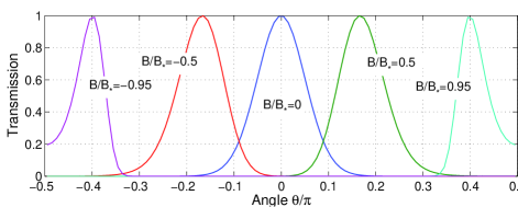
Figure 2: Angular dependence of transmission for different magnetic field values, $T(\theta)=e^{-\alpha\gamma^{3}(\sin\theta-B/B_{\ast})^{2}}$, Eq.(15), for $\alpha=\pi(d/\lambdabar_{F})^{2}=20$. Transmission reaches unity at a field-dependent angle $\theta_{B}=\arcsin B/B_{\ast}$.

The dependence of the transparency (15) on the electric field $E$ is such that $T$ grows as $E$ increases. This is a manifestation of the Klein tunneling phenomenon in which steeper barriers yield higher transmission.

The result (15) features exponential suppression of tunneling by $B$ field for all momenta except $p_{1}=-\beta\varepsilon$ that yields perfect transmission. This corresponds to the incidence angle $\theta_{B}=\arcsin B/B_{\ast}$ (see Fig.2). At equal p and n densities, the velocities of transmitted particles are collimated at $\theta\approx\theta_{B}$, with the collimation angle variance determined by $\Delta p_{1}\approx d^{-1}\gamma^{-3/2}$. This gives an estimate

$$\Delta\theta\sim(\lambdabar/d)\left(1-(B/B_{\ast})^{2}\right)^{1/4},\quad\lambdabar=v_{F}/\varepsilon_{F}.$$ (16)

We conclude that the nearly unit transmission, which occurs perpendicular to the p-n interface at $B=0$ Katsnelson06b ; Cheianov06 , persists at finite magnetic fields, albeit for $\theta_{B}\neq 0$. This behavior of the collimation angle can be used to realize a switch (see Fig.3), in which current is channeled between diferent pairs of contacts by varying the $B$ field.

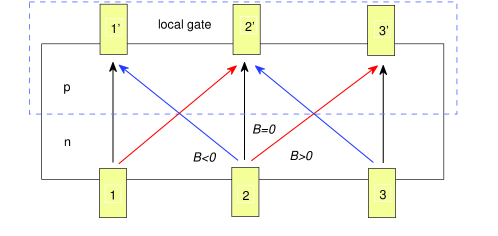
Figure 3: Field-controled switching of collimated current flow through a ballistic p-n junction between different contacts.

The p-n junction net conductance can be found from the Landauer formula

$$G=\frac{e^{2}}{h}\sum_{-k_{F}<p_{1}<k_{F}}T(p_{1})=\frac{we^{2}}{2\pi h}\int_{-k_{F}}^{k_{F}}T(p_{1})dp_{1}$$ (17)

where $w$ is the length of the junction interface (see Fig.1), and the states contributing to transport are those at the Fermi level, $\varepsilon=\varepsilon_{F}$. For a wide junction, $w\gg d\gg\lambdabar_{F}$, extending integration over $p_{1}$ to infinity we obtain the $\left(1-(B/B_{\ast})^{2}\right)^{3/4}$ dependence (2).

It is interesting to apply these results to epitaxial graphene, described by massive Dirac particles $\varepsilon=\pm(v_{F}^{2}{\bf p}^{2}+\Delta^{2})^{1/2}$ with an energy gap $\Delta$ induced by the substrate Lanzara ; Mattausch07 . The generalization amounts to replacing $p_{1}^{2}$ by $p_{1}^{2}+\Delta^{2}/v_{F}^{2}$ in (6). Performing Lorentz transformation, we find exponential suppression of conductance:

$$G(B)=\frac{e^{2}}{2\pi h}\frac{w}{d}\left(1-\beta^{2}\right)^{3/4}\textstyle{\exp\left(-\frac{\pi d^{2}\Delta^{2}}{v_{F}^{2}(1-\beta^{2})^{1/2}}\right)}$$ (18)

(cf. Refs.AronovPikus66 ; Weiler67 ). The angular dependence of transmission in this case is the same as in the massless case.

We note that $G(B\geq B_{\ast})=0$ does not necessarily mean that the system ceases to conduct. The behavior predicted by Eq.(2) at $B\geq B_{\ast}$ should be interpreted as 2D transport pinching off by the onset of the Quantum Hall effect. In that, just the part of the conductance proportional to the sample width $w$ vanishes, while the edge mode contribution remains nonzero.

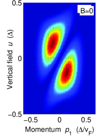
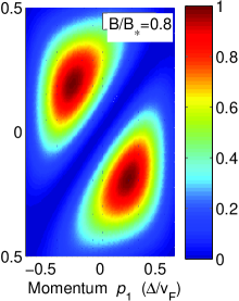
Figure 4: Transmission of a bilayer p-n junction vs. momentum parallel to the interface and vertical field. Note the double hump structure with unit transmission at the peak, and suppression of tunneling at large $u$ and $p_{1}$ ($E^{\prime}=0.05\Delta^{2}/ev_{F}$).

Our approach can be readily generalized to described recently fabricated p-n junctions in graphene bilayers Oostinga07 . The bilayer Hamiltonian McCann06 includes the standard monolayer tight-binding part, as well as a direct coupling between the adjacent sites $B$, $\tilde{A}$ of different monolayers and a weaker coupling between non-adjacent sites $A$, $\tilde{B}$: $\gamma_{\tilde{B}A}\ll\gamma_{B\tilde{A}}\approx 0.6\,{\rm eV}$ in notation of Ref.McCann06 . Here, for simplicity, we ignore $\gamma_{\tilde{B}A}$ and denote $\gamma_{B\tilde{A}}$ as $\Delta$.

It is convenient to write the bilayer Hamiltonian, linearized near the Dirac points, in pseudospin notation, using $\tau_{3}=\pm 1$ to label the monolayers. The inter-layer coupling takes the form $H_{\Delta}=\Delta\left(\tau_{+}\sigma_{-}+\tau_{-}\sigma_{+}\right)=\frac{\Delta}{4}\left(\tau_{1}\sigma_{1}+\tau_{2}\sigma_{2}\right)$, where $\sigma_{\pm}=\frac{1}{2}(\sigma_{1}\pm i\sigma_{2})$, $\tau_{\pm}=\frac{1}{2}(\tau_{1}\pm i\tau_{2})$. This gives the Hamiltonian

$$H=v_{F}p_{1}\sigma_{1}-v_{F}p_{2}\sigma_{2}+\frac{1}{2}u\tau_{3}+\frac{\Delta}{2}\left(\tau_{1}\sigma_{1}+\tau_{2}\sigma_{2}\right),$$ (19)

where $u$ is the vertical field that opens a gap of size $|u|$ in the bilayer spectrum. Multiplying the time-dependent Schrödinger equation by $\sigma_{3}$, we rewrite it as a Dirac equation (7) with a fictitious $\tau$-dependent gauge field:

$$\gamma^{\mu}(p_{\mu}-a_{\mu}-g_{\mu})\psi=0,\quad g_{\mu}=\left(\tilde{u}\tau_{3},-\tilde{\Delta}\tau_{1},\tilde{\Delta}\tau_{2}\right),$$ (20)

where $\tilde{u}=u/2v_{F}$, $\tilde{\Delta}=\Delta/2v_{F}$, and the external field $a_{\mu}$ is defined in the same way as above.

Under Lorentz boost (14) the equation $\gamma^{\mu}(p_{\mu}-a_{\mu}-g_{\mu})=0$ changes covariantly with the momenta and fields transforming via $p^{\prime}=\Lambda p$, $a^{\prime}=\Lambda a$, $g^{\prime}=\Lambda g$, giving $g_{\mu^{\prime}}=\frac{1}{2v_{F}}\left(\gamma(u\tau_{3}-\beta\Delta\tau_{1}),\gamma(\beta u\tau_{3}-\Delta\tau_{1}),\Delta\tau_{2}\right)$. Choosing $\beta$ so as to eliminate the $B$ field, we find the transformed Hamiltonian $H^{\prime}=-eE^{\prime}x_{2}+H_{k}(p^{\prime}_{1},p^{\prime}_{2})$, where

$$H_{k}(p^{\prime}_{1},p^{\prime}_{2})=\frac{1}{2}\gamma\left(u\tau_{3}-\beta\Delta\tau_{1}\right)+$$ (21)

$$\left(v_{F}p^{\prime}_{1}-\frac{1}{2}\gamma(\beta u\tau_{3}-\Delta\tau_{1})\right)\sigma_{1}-\left(v_{F}p^{\prime}_{2}-\frac{1}{2}\Delta\tau_{2}\right)\sigma_{2}.$$

Working in the momentum representation, as above, we treat $\varepsilon^{\prime}\psi^{\prime}=H^{\prime}\psi^{\prime}$ as a first-order differential equation

$$ieE^{\prime}\,d\psi/dp^{\prime}_{2}=\left(H_{k}(p^{\prime}_{1},p^{\prime}_{2})-\varepsilon^{\prime}\right)\psi.$$

We evaluate the transfer matrix of this equation numerically, and find that in the physically interesting case $u\ll\Delta$, the lowest and the uppermost energy levels of $H_{k}$ are decoupled from the two middle levels. The $4\times 4$ transfer matrix is thus reduced to a $2\times 2$ matrix, yielding the transmission and reflection coefficients.

Transmission features an interesting behavior as a function of external fields and particle momentum (see Fig.4). It has a symmetric double hump profile as a function of $p_{1}$ and $u$ vanishing between the humps (unlike single gaussian peak in the monolayer case) and, somewhat unexpectedly, perfect transmission at the peak. At large $p_{1}$ and $u$, because of the energy gap opening, transmision is strongly suppressed. Conductance, found from the Landauer formula (17), also exhibits strong suppression at increasing $u$ and $B$, qualitatively similar to the gapped monolayer case, Eq.(18).

We benefited from useful discussions with C. M. Marcus and D. A. Abanin. This work is supported by the DOE (contract DEAC 02-98 CH 10886), NSF MRSEC (DMR 02132802) and NSF-NIRT DMR-0304019.

References

- (1) B. Huard et al., Phys. Rev. Lett. 98, 236803 (2007).
- (2) J. R. Williams, L. C. DiCarlo, C. M. Marcus, Science 317, 638 (2007).
- (3) B. Özyilmaz et. al., cond-mat/0705.3044
- (4) M. I. Katsnelson, K. S. Novoselov, A. K. Geim, Nat. Phys. 2, 620 (2006).
- (5) M. I. Katsnelson and K. S. Novoselov, Sol. St. Comm. 143, 3 (2007).
- (6) V. V. Cheianov and V. I. Falko, Phys. Rev. B 74, 041403 (2006).
- (7) V. V. Cheianov, V. I. Fal’ko, and B. L. Altshuler, Science 315, 1252 (2007).
- (8) D. A. Abanin and L. S. Levitov, Science 317, 641 (2007).
- (9) L. D. Landau and E. M. Lifshitz, Classical Theory of Fields, (3rd ed., Pergamon, London 1971).
- (10) A. G. Aronov and G. E. Pikus, Sov. Phys. JETP 24, 188 (1967); 339 (1967).
- (11) M. H. Weiler, W. Zawadzki, and B. Lax, Phys. Rev. 163, 733 (1967).
- (12) V. Lukose, R. Shankar, and G. Baskaran, Phys. Rev. Lett. 98, 116802 (2007).
- (13) A. H. MacDonald, Phys. Rev. B 28, 2235 (1983).
- (14) L. M. Zhang and M. M. Fogler, arXiv:0708.0892
- (15) E. O. Kane and E. Blount, in: Tunneling Phenomena in Solids, ed. by E. Burstein and S. Lundqvist (Plenum Press, New York, 1969).
- (16) A. V. Andreev, arXiv:0706.0735v1
- (17) L. D. Landau and E. M. Lifshitz, Quantum Mechanics, Chap. XI, §90 (3rd ed., Pergamon, London 1977).
- (18) A. Lanzara, private communication.
- (19) A. Mattausch and P. Pankratov, arXiv:0704.0216
- (20) J. B. Oostinga et al., arXiv:0707.2487
- (21) E. McCann and V. I. Fal’ko, Phys. Rev. Lett. 98, 086805 (2006).