Quantum Communication
Non-classical correlations and their applications

Abstract

Communication is transfer of information. Compared to classical physics, new possibilities arise when information is encoded in quantum systems and processed with quantum operations.

In the first part of this thesis Bell’s theorem is revisited. It points at a difference between the quantum and the classical world. This difference is often behind the advantages of solutions using quantum mechanics. New and more general versions of Bell inequalities are presented. These inequalities involve multiple settings per observer. Compared with the two-setting inequalities, the new ones reveal the nonclassical character of a broader class of states. Some of them are also proven to be optimal (tight).

Next, we go beyond Bell’s theorem. It is shown, both in theory and in experiment, that incompatibility between quantum mechanics and realistic theories can be extended into an important class of nonlocal models. We also show that the violation of Bell inequalities disqualifies local realistic models with a limited lack of the experimenter’s freedom. This, at first glance quite philosophical result, has its down-to-earth implications for quantum communication.

In the second part of the thesis well-known examples of quantum communication are reviewed. Next, new results concerning quantum cryptography and quantum communication complexity are given.

Publications

This work is based on the following publications:

• S. Gröblacher, T. Paterek, R. Kaltenbaek, Č. Brukner, M. Żukowski, M. Aspelmeyer, and A. Zeilinger
  An experimental test of non-local realism
  Nature 446, 871 (2007).

• T. Paterek
  Measurements on composite qudits
  Phys. Lett. A 367, 57 (2007).

• K. Nagata, W. Laskowski, and T. Paterek
  Bell inequality with an arbitrary number of settings and its applications
  Phys. Rev. A 74, 62109 (2006).

• J. Kofler, T. Paterek, and Č. Brukner
  Experimenter’s freedom in Bell’s theorem and quantum cryptography
  Phys. Rev. A. 73, 22104 (2006).

• T. Paterek, W. Laskowski, and M. Żukowski
  On series of multiqubit Bell’s inequalities
  Mod. Phys. Lett. A. 21, 111 (2006).

• W. Laskowski, T. Paterek, M. Żukowski, and Č. Brukner
  Tight multipartite Bell’s inequalities involving many measurement settings
  Phys. Rev. Lett. 93, 200401 (2004).

• Č. Brukner, T. Paterek, and M. Żukowski
  Quantum communication complexity protocols based on higher-dimensional entangled systems
  Int. J. Quant. Inf. 1, 519 (2003).

Acknowledgements

I would like to thank Professor Marek Żukowski for opening me a completely new world. Many thanks to my friends from the groups of Gdańsk and Vienna.

This research was supported by several institutions (in chronological order):

• University of Gdańsk
  Stipend for Ph. D. students
  Grant No. BW/5400-5-0256-3

• Austrian-Polish projects Quantum Communication and Quantum Information

• German-Polish project Novel Entangled States for Quantum Information Processing: Generation and Analysis

• Foundation for Polish Science
  Stipends under the Professorial Subsidy of Marek Żukowski

• State Committee for Scientific Research
  Grant No. PBZ-MIN-008/P03/03
  Grant No. 1 P03B 04927

• The Erwin Schrödinger International Institute for Mathematical Physics
  Junior Research Fellowship

• European Union
  QAP programme Contract No. 015848

Chapter 1 Introduction and summary

1.1 Introduction: field of quantum communication

We are living in the age of information. One can safely state that the rapid progress of the last century was connected with a growing accessibility of information. In turn, this accessibility is linked with the discoveries of the secrets of nature. Many of them were secrets of quantum physics. Quantum physics may influence our everyday life soon. Many technological developments reach the scale of its applicability. Already today it is estimated that quite a big part of our tools can be designed only due to our knowledge of quantum mechanics. For example, if the progress in the power of personal computers is going to stay at the current level (doubles itself every two years – the so called Moore’s law) quantum effects inevitably start to dominate in the processors soon.

Information and physics cannot be divided. Information is an intrinsically physical concept. It relies on physical systems in which information is stored and by means of which information is processed or transmitted. Transmission of information encoded in quantum systems and processed by operations allowed by quantum mechanics is studied in the field of quantum communication.

Quantum communication is a relatively new sub-branch of physics and information theory. Its main goals include a theory of optimal encoding and decoding of information into quantum systems, and their faithful transmission through (possibly noisy) communications channels. It is also aimed at showing communication tasks which are either impossible in classical regime or their quantum versions outperform the best classical solution. At least one of such protocols, quantum cryptography, is already at the stage of useful real-world applications.

Quantum cryptography allows secure communication. Communication which guarantees that transmitted information is inaccessible to third parties. The security is due to the laws of quantum physics. Any disturbance of a quantum system, inevitably caused by an eavesdropper, changes a state of the system. This change can in principle be detected by legitimate partners. Classical crypto-algorithms up to date make use of problems which are believed to be computationally hard. Despite of many attempts it is not proven that classical cryptography cannot be compromised. Moreover, there exist a quantum algorithm (Shor’s algorithm) which efficiently solves problems at the heart of classical cryptography (believed to be classically hard). Thus, quantum cryptography may one day dominate on the market. There are also attempts to unify cryptography and computation and there already are proposals for secure computation.

There is an ongoing debate on which are the properties of quantum physics that allow to derive benefit from using ”quantum” in information processing. The correlations allowed by quantum mechanics seem to be a good candidate. The correlations between quantum particles can be much stronger than the correlations between classical objects. These non-classical correlations are due to quantum entanglement. Although there exist superior quantum protocols which make use of no entanglement, this purely quantum resource is usually sufficient for better performance of quantum algorithms. As soon as one recognizes that a problem requires correlations similar to those of quantum entanglement, most probably the problem has efficient quantum solution utilizing a suitable entangled state.

For example, in the field of communication complexity (introduced in $1979$ by Yao) one can show problems with quantum solutions which outperform any classical ones. In a communication complexity problem, separated parties performing local computations exchange information in order to accomplish a globally defined task, which is impossible to solve singlehandedly. These problems find applications in optimization of data structures or minimization of time required to perform a computation with large integrated circuits. An instance of a communication complexity problem is evaluation of a function dependent on distributed inputs. Imagine every party receives two bits in such a way that they do not know the bits of any other party. Their common goal is to compute a value of a function defined on all the bits. However, each party can communicate only one bit. Before parties receive their inputs they can communicate freely. They can fix the protocol they will use once the data is obtained, they can share some correlated strings of numbers in the classical scenario or entangled states in the quantum case. The communication starts to be “expensive” with the delivery of the bits. The essence of quantum solutions to communication complexity problems is to share an entangled state before parties receive their inputs. The state is such that when suitably measured gives correlated results in agreement with the function to be computed. When the bits are delivered, parties make local measurements depending on their local inputs, next they communicate local outcomes (assumed to be bits in our example), and give as the computed value of the function the product of all local results. There are functions for which this protocol is more efficient in terms of communication complexity than the best classical protocol. Evidently, the quantum protocol is linked with the entanglement.

Generally, it is a very hard problem to decide whether a quantum state is entangled or not. The problem seems to be even more difficult when experimental data is taken into account. It can happen that it is not even clear which quantum state describes the data. Fortunately, there are operational criteria (entanglement witnesses), relying on measurements of correlations, with a possible outcome from which one can conclude that the state is entangled.

One of such witnesses is a Bell inequality. A Bell inequality is satisfied by all states which are not entangled. Thus, if a violation of a Bell inequality is observed the state which describes the results is entangled. Interestingly, Bell inequalities were first introduced in a context of foundations of quantum mechanics. They represent constraints on correlations which must be fulfilled by all models which are based on the classical concepts and the principle of relativistic causality. With the emergence of quantum information Bell inequalities found new applications. Limits of performance of certain classical protocols (e.g. already mentioned communication complexity protocols) can be described in a form of a Bell inequality. Since entangled states violate Bell inequalities it is clear that quantum protocols can beat classical limits. In this way, human philosophical curiosity has found applications in applied science.

The link between physics and information also brings new insight into physics itself. It is always good to view problems from different perspectives. Quantum information puts forward such a new perspective.

1.2 Summary of the results

In the first part of this dissertation Bell’s theorem is revisited. The evolution of Bell inequalities is described. We starting with the problem of the possibility of local realistic models of quantum predictions, which was posed by Einstein, Podolsky and Rosen [1]. Next, we scan through some known versions of Bell’s impossibility theorem [2, 3, 4, 5], and finish with the necessary and sufficient condition for the local realistic description of correlation experiments performed on many qubits [7, 8, 9]. Next, basing on the assumptions of Bell, we present new multisetting inequalities for many qubits [P3,P5,P6]. The inequalities are derived using two different techniques. Inequalities [P5,P6] are proven to be optimal but they cannot involve arbitrary number of settings per party. The other inequalities [P3] incorporate in a compact form any number of settings per party, but they are not always optimal. In both cases, we derive conditions for violation of the inequalities and present examples of states which (do not) violate them. It is shown that the multisetting inequalities reveal non-classical character of certain states which satisfy all two-setting Bell inequalities with correlation functions [7, 8, 9].

Violation of Bell inequalities was observed in many experiments. The results agree with quantum predictions (the milestones are those of [10, 11, 12, 13]). Certain loopholes are known to exist which still allow to explain experimental data in a local realistic way. However, these were all separately closed in the cited experiments. Thus, the violation of local realism is usually considered as a well established fact. We go beyond Bell’s assumptions and describe a class of nonlocal realistic theories still incompatible with quantum mechanics. This class was introduced by Leggett [14]. We have also performed an experiment with entangled photons which disqualifies this class of theories. This was the first experimental demonstration which invalidates some nontrivial nonlocal realistic models. The considered theories (i) model all experiments in which a violation of two-setting Bell inequalities (e.g. the widely studied CHSH inequality [3]) is observed; (ii) model perfect correlations in the complementary bases, which is the feature of the Bell singlet state; (iii) although nonlocal do not allow to transmit information faster than speed of light [P1].

In an independent line of research we have relaxed, often tacit in the derivation of Bell inequalities, the “free-will” assumption [15, 16]. This assumption is essential for Bell experiments, as lack of freedom to choose between different experimental arrangements allows one to explain a violation of Bell inequalities within local realism. We argue that within a local realistic model this freedom can experimentally be checked. If one wants to keep such a picture, the experimental evidence of a violation of Bell inequalities sets the minimal amount to which the freedom has to be abandoned.

In the second part of the thesis some examples of the superiority of quantum communication are presented. We review quantum teleportation [17], quantum dense coding [18], quantum cryptography [19, 20, 21], and quantum communication complexity [22, 23]. In the last two fields, both linked with Bell’s theorem, new results are presented.

In the case of quantum cryptography we show, following the freedom considerations, that one can relax to some extend the assumption that laboratories of authenticated parties are not vulnerable and still secure quantum key distribution is possible [P4]. It is also shown that quantum cryptography with higher-dimensional quantum systems [24], proven to be more secure than qubit-based protocol, is relatively easy to realize using system composed of two subsystems [P2].

In the field of quantum communication complexity we present the general link between Bell inequalities for qubits and communication complexity problems [23], associated with one of the multisetting inequalities [P3]. Next, we construct a communication complexity task for higher-dimensional quantum systems [P7]. The quantum solution outperforms a broad class of classical protocols and it may be conjectured, based on the recent results for qubits [25], that the class of classical solutions includes the optimal one.

Chapter 2 Non-classical correlations

This part of the thesis is devoted to Bell’s theorem [2]. It states that no local realistic (classical) model exists which explains all quantum predictions. Thus, Bell’s discovery points at a difference between the quantum and the classical world. Some conditions necessary for the local realistic models are given in form of Bell inequalities. Quantum states which violate these inequalities are a valuable resource in quantum communication and quantum information processing in general [26].

First we present a brief history of Bell’s discovery and a few well-known versions of his theorem. Further on, a new family of tight (optimal) Bell inequalities is discussed, which enlarges the class of quantum states that do not admit a local hidden-variable (realistic) description. Next, we give a compact formula for Bell inequalities involving an arbitrary number of measurement settings and an arbitrary number of observers. Many previously known inequalities are special cases of this general one. We also present the violation conditions for these inequalities and examples of states which (do not) violate them.

In the following section it is proven, and experimentally confirmed, that quantum mechanical predictions are incompatible with certain plausible classes of nonlocal hidden-variable theories. This program was initiated by Leggett [14].

We also relax the assumption of experimenter’s freedom to choose between different measurement settings. A measure of the lack of this freedom is developed, and the minimal extend of this lack, which allows to explain the violation of Bell inequalities within a local realistic picture, is derived.

2.1 Overview of earlier works on Bell’s theorem

2.1.1 Bell’s theorem

Quantum mechanics gives predictions in form of probabilities. Already some of the fathers of the theory were puzzled with the question whether there can exist a deterministic structure beyond quantum mechanics which recovers quantum statistics as averages over “hidden variables” (see a beautiful review by Clauser and Shimony [27]). In this way, it was hoped, one could get a classical-like description which would solve the problems with the interpretations of quantum mechanics. In his famous impossibility proof Bell made precise assumptions about the form of a possible underlying hidden variable structure. Spatially separated systems and laboratories were assumed to be independent of one another [2]. He derived an inequality which must be satisfied by all such (local realistic) structures. Next, he presented example of quantum predictions which violate it. In this way the famous Einstein-Podolsky-Rosen (EPR) paradox [1] was solved. Bell proved that EPR elements of reality cannot be used to describe quantum mechanical systems.

The noncommutativity of quantum theory precludes simultaneous deterministic predictions of measurement outcomes of complementary observables. For EPR this indicated that “the wave function does not provide a complete description of physical reality”. They expected the complete theory to predict outcomes of all possible measurements, prior to and independent of the measurement (realism), and not to allow “spooky action at a distance” (locality). Such a completion was disqualified by Bell.

A more general version of Bell’s theorem for two qubits (two-level systems) was given by Clauser, Horne, Shimony, and Holt (CHSH), and extended by Clauser and Horne (CH) [3, 4]. The important feature of the CHSH and CH inequalities, which hold for all local realistic theories, is that they can not only be compared with ideal quantum predictions, but also with experimental results. Thus, a debate that seemed quasi-philosophical could be moved into the lab!

The three or more qubit versions of Bell’s theorem were presented by Greenberger, Horne, and Zeilinger (GHZ), surprisingly $25$ years after the original paper of Bell [5, 6]. In contradistinction with the two particle case, now the contradiction between local realism and quantum mechanics could be shown for perfect correlations. Immediately after that, Mermin produced a series of inequalities for arbitrary many particles, which cover the GHZ case, and made the GHZ paradox directly testable in the laboratory [28]. A complementary series of inequalities was introduced by Ardehali [29]. In the next step Belinskii and Klyshko gave series of two-settings inequalities, which contained the tight inequalities of Mermin and Ardehali [30]. Finally, the full set of tight two-setting Bell inequalities for dichotomic observables, involving correlations between $N$ partners, was described independently by Werner and Wolf [7], and in the papers by Weinfurter and Żukowski [8], and Żukowski and Brukner [9].

Intuitively, one would link the violation of Bell inequalities with entanglement. Indeed, only entangled states can violate them. Surprisingly, there are pure entangled states whose multiparticle correlations, obtained in a two-setting Bell experiment, can be modelled in a local realistic way [31]. To reveal non-classical behaviour of such states one needs to perform Bell experiments with many settings per party. Various methods were proposed to obtain multisetting inequalities [32, 33, 34, 35, 36, 37, 38, 39, 40]. Here, we present the simple and efficient method of [P6]. It allows a derivation of tight Bell inequalities involving various combinations of the number of settings per party, and an arbitrary number of parties. Finally, an inequality incorporating an arbitrary number of settings and arbitrary number of observers is given [P3]. However, this inequality is not always tight.

2.1.2 Einstein-Podolsky-Rosen

In their original paper Einstein, Podolsky, and Rosen (EPR) considered quantum predictions for measurements of position and momentum [1]. We explain their reasoning with a simpler example of two maximally entangled qubits. This approach was first presented by Bohm [41].

EPR assume there exists an objective reality independent of any physical theory. Theoretical concepts help us to understand this reality, “by means of these concepts we picture this reality to ourselves”. By EPR the necessary condition for completeness of a physical theory is that every element of physical reality must have a counterpart in the physical theory. Next, they define elements of physical reality in the following way: If, without in any way disturbing the system, we can predict with certainty (i.e., with probability equal to one) the value of a physical quantity, then there exists an element of physical reality corresponding to this physical quantity. Within these definitions quantum theory seems to be incomplete because according to EPR one can show the existence of elements of physical reality, whereas quantum mechanics does not use this concept.

Consider two observers, Alice and Bob, in two distant laboratories [Fig. 2.1]. They perform measurements on spin-$\frac{1}{2}$ particles which used to interact in the past. The quantum mechanical description of their joint state of spins reads:

$$|\psi^{-}\rangle=\frac{1}{\sqrt{2}}\Big{[}|z+\rangle_{A}|z-\rangle_{B}-|z-\rangle_{A}|z+\rangle_{B}\Big{]},$$ (2.1)

where $|z+\rangle$ and $|z-\rangle$ denote the eigenstates of the $(\sigma_{3}\equiv)\sigma_{z}$ operator. The remarkable property of the state (2.1) is its invariance under the same rotations of observables in the two labs. In particular, if Alice and Bob measure the same observable, whatever outcome of Alice, the outcome of Bob is always opposite. If Alice measures $\sigma_{z}$ then she can predict with certainty the outcome of Bob’s $\sigma_{z}$ measurement. Thus, according to EPR there exists an element of physical reality connected with the $\sigma_{z}$ measurement. Just as well Alice could measure $(\sigma_{1}\equiv)\sigma_{x}$ and predict with certainty, without in any way disturbing the system, the outcome of a possible $\sigma_{x}$ measurement by Bob. Again, seemingly there exists an element of reality connected with the $\sigma_{x}$ measurement. Locality is assumed here: the physical reality at Bob’s site is independent of everything that happens at Alice’s site. Since quantum mechanics does not allow simultaneous knowledge of both $\sigma_{x}$ and $\sigma_{z}$, it misses some concepts which are necessary for the theory to be complete.

2.1.3 Bell and Clauser-Horne-Shimony-Holt

Twenty nine years after the EPR paper, Bell proved that the completion of quantum mechanics expected by EPR is impossible [2]. In his original proof Bell utilized the perfect anticorrelations, which arise whenever Alice and Bob measure local spins (with respect to the same direction) on the two-qubit system in the state (2.1). However, unavoidable experimental imperfections imply that correlations are never perfect. To illustrate the essence of Bell’s theorem we re-derive the CHSH inequality [3]. The validity of this inequality does not require perfect correlations and thus it can be directly experimentally checked.

Figure 2.1: EPR-Bell gedanken experiment. Two distant observers (Alice and Bob) measure particles which used to interact in the past. Alice and Bob choose between two alternative settings of the local measurement apparatuses.

Consider the experiment proposed by EPR [Fig. 2.1] and studied by Bell. The pair emission begins an experimental run. In each run Alice and Bob can choose between two alternative settings of the local measurement apparatuses. Their choices what to measure are absolutely free, uncorrelated with (statistically independent of) the operation of the source. According to realism the outcomes of all possible measurements exist prior to and independent of the acts of measurement. Locality assumes that the outcomes of Alice depend on her setting only, and the same for Bob. For a given run, denote the predetermined local realistic results as $A_{1}$, $A_{2}$ for Alice, and $B_{1}$, $B_{2}$ for Bob. For example, if Alice chooses to measure setting “1” she obtains outcome $A_{1}$, if she chooses to measure “2” she obtains $A_{2}$. Under the assumption of realism the outcomes of all possible measurements are defined, even if only some of them are actually measured. Experiments on qubits can give one of two results, to which we ascribe numbers, $+1$ and $-1$, i.e. $A_{k},B_{l}=\pm 1$, with indices $k,l=1,2$ denoting the settings. The following identity holds in every experimental run:

$$A_{1}(B_{1}+B_{2})+A_{2}(B_{1}-B_{2})=\pm 2.$$ (2.2)

All variables in this expression are dichotomic (of values $\pm 1$), thus either $B_{1}+B_{2}=\pm 2$ and $B_{1}-B_{2}=0$, or the other way around.

After averaging over many experimental runs expression (2.2) reads:

$$-2\leq\langle A_{1}B_{1}+A_{1}B_{2}+A_{2}B_{1}-A_{2}B_{2}\rangle\leq+2.$$ (2.3)

The bounds follow from the fact that with averaging one cannot exceed the extremal values of the averaged expression. Since the average of a sum is a sum of averages, the last inequality transforms to:

$$\Big{|}\langle A_{1}B_{1}\rangle+\langle A_{1}B_{2}\rangle+\langle A_{2}B_{1}\rangle-\langle A_{2}B_{2}\rangle\Big{|}\leq 2.$$ (2.4)

Note that within realistic theories a single experimental run contributes to all averages in this expression. After $R$ runs, the average of the product of predetermined results, the local realistic correlation function, reads:

$$E_{kl}^{LR}\equiv\langle A_{k}B_{l}\rangle=\frac{1}{R}\sum_{n=1}^{R}A_{k}^{(r)}B_{l}^{(r)},$$ (2.5)

where $A_{k}^{(r)}$, $B_{l}^{(r)}$ denote the predetermined results in the $r$th run. Finally, one arrives at the famous Clauser-Horne-Shimony-Holt inequality [3]:

$$S_{CHSH}\equiv\Big{|}E_{11}^{LR}+E_{12}^{LR}+E_{21}^{LR}-E_{22}^{LR}\Big{|}\leq 2,$$ (2.6)

which is satisfied by the correlations of all local realistic models.

To complete the proof of Bell’s theorem, let us give an example of quantum predictions which violate the CHSH inequality. One replaces the local realistic correlation functions in (2.6) with their quantum counterparts, $E_{kl}^{QM}$, for the singlet state (2.1). The quantum correlation function reads (Appendix A):

$$E_{kl}^{QM}=-\vec{a}_{k}\cdot\vec{b}_{l},$$ (2.7)

where dot stands for a scalar product between vectors $\vec{a}_{k}$ and $\vec{b}_{l}$, which parameterize the measurement settings of Alice and Bob, respectively. Thus, quantum mechanics predicts for the left-hand side of (2.6):

$$S_{CHSH}^{QM}=\Big{|}-\vec{a}_{1}\cdot\vec{b}_{1}-\vec{a}_{1}\cdot\vec{b}_{2}-\vec{a}_{2}\cdot\vec{b}_{1}+\vec{a}_{2}\cdot\vec{b}_{2}\Big{|},$$ (2.8)

which can be directly transformed to:

$$S_{CHSH}^{QM}=\Big{|}\vec{a}_{1}\cdot(\vec{b}_{1}+\vec{b}_{2})+\vec{a}_{2}\cdot(\vec{b}_{1}-\vec{b}_{2})\Big{|}.$$ (2.9)

We are looking for a maximum of this expression. Since the $\vec{b}_{k}$ vectors are normalized, the vectors in the brackets are orthogonal:

$$(\vec{b}_{1}+\vec{b}_{2})\cdot(\vec{b}_{1}-\vec{b}_{2})=|\vec{b}_{1}|^{2}-|\vec{b}_{2}|^{2}=0.$$ (2.10)

Further, note that:

$$|\vec{b}_{1}+\vec{b}_{2}|^{2}+|\vec{b}_{1}-\vec{b}_{2}|^{2}=2(|\vec{b}_{1}|^{2}+|\vec{b}_{2}|^{2})=4.$$ (2.11)

Thus, one can parameterize the length of these vectors with a single angle, $\alpha$. Finally, one can introduce normalized orthogonal vectors $\vec{b}_{+}$ and $\vec{b}_{-}$ such that:

$$\vec{b}_{1}+\vec{b}_{2} = 2\cos\alpha\textrm{ }\vec{b}_{+},$$ (2.12)

$$\vec{b}_{1}-\vec{b}_{2} = 2\sin\alpha\textrm{ }\vec{b}_{-}.$$ (2.13)

Using this decomposition, expression (2.9) transforms to:

$$S_{CHSH}^{QM}=\Big{|}2\cos\alpha\textrm{ }\vec{a}_{1}\cdot\vec{b}_{+}+2\sin\alpha\textrm{ }\vec{a}_{2}\cdot\vec{b}_{-}\Big{|}.$$ (2.14)

The scalar products are maximal (and equal to one) if one chooses $\vec{a}_{1}=\vec{b}_{+}$ and $\vec{a}_{2}=\vec{b}_{-}$. After this choice one needs to find a maximum of $2|\cos\alpha+\sin\alpha|$. The maximum is attained for $\alpha=\pi/4$, and gives a corresponding maximal quantum value for the CHSH expression

$$S_{CHSH}^{QM}(max)=2\sqrt{2},$$ (2.15)

clearly above the local realistic bound of $2$. This value was confirmed in numerous experiments, e.g. [10, 11, 12, 13].

To reach the maximal violation one constraints the measurement vectors for Alice and for Bob to lie in the same plane. In this case the quantum correlation function can be written as

$$E_{kl}^{QM}=-\cos(\varphi_{k}^{A}-\varphi_{l}^{B}),$$ (2.16)

where $\varphi_{k}^{A}$ and $\varphi_{l}^{B}$ parameterize the position of the measurement vectors within the plane, relative to some fixed axis. The maximum is achieved, for example, if Alice sets her angles to

$$\varphi_{1}^{A}=0,\quad{\rm and}\quad\varphi_{2}^{A}=\pi/2,$$ (2.17)

and Bob sets his angles to

$$\varphi_{1}^{B}=\pi/4,\quad{\rm and}\quad\varphi_{2}^{B}=-\pi/4.$$ (2.18)

2.1.4 Assumptions

Let us gather together the assumptions behind the derivation of Bell inequalities, and their experimental tests.

To derive the CHSH inequality (2.6) one assumes:

• realism
  Unperformed measurements have well-defined, yet unknown, results.

  A picture behind realism is that there exist objective properties of particles, which predetermine measurement outcomes. These properties, as well as the properties of the measurement apparatus, are described by hidden variables.

• locality
  Measurement outcomes at one location depend on the measurement setting in this location only.

In the experimental tests of Bell inequalities an additional assumption is unavoidable:

• freedom
  Statistical independence between the choice of measurement settings and the workings of the source.

  It is assumed that the correlations measured, given the settings $k$ and $l$, are the same up to insignificant statistical fluctuations as the hypothetical local realistic correlations $E_{kl}^{LR}$ (cf. section on experimenter’s freedom). Otherwise one could not derive the inequality:

  $$|E_{11}+E_{12}+E_{21}-E_{22}|\leq 2,$$ (2.19)

  in which the experimental correlations appear.

  Note that this assumption is fundamental, and cannot be removed in any experimental setup.

2.1.5 Loopholes

Additionally, there exist certain experimental imperfections which still allow to describe measured correlations in a local realistic way. Although there is no experiment up to date which closes all these loopholes simultaneously, every loophole was closed in separate experiments. Therefore, it is unlikely that a “final” test would fail. However, as usual in physics, final verdict belongs to experiment.

• locality loophole
  A natural locality requirement comes from the relativity theory. If the detection event of, say, Bob lies within a light-cone initiated by the choice of the measurement setting of Alice, the outcome of Bob can be a function of the setting of Alice. Arbitrary violation of inequality (2.6) can be explained in this case since the identity (2.2) no longer holds. Instead one has:

  $$A_{11}B_{11}+A_{12}B_{21}+A_{21}B_{12}-A_{22}B_{22},$$ (2.20)

  where $A_{kl}$ and $B_{lk}$ are functions of both, the settings of Alice and Bob. This identity can achieve even the value of four. One simply sets $B_{11}=B_{21}=B_{12}=-B_{22}=1$ and $A_{11}=A_{12}=A_{21}=A_{22}=1$.

  There is a subtle issue connected to the locality loophole. In the famous experiment of Aspect [11] the settings were chosen during the flight of the photons such that detection event and the choice of the settings were separated by a spacelike interval. However, in this experiment the measurement choices were predictable. In principle, one can build a local hidden variable model taking advantage of this predictability and again the outcomes of Bob could effectively depend on the setting of Alice. This possibility was disproved in the Innsbruck experiment, in which it is impossible to predict the settings in advance, due to their inherent randomness [12].

• detection loophole
  Most of the experiments testing Bell inequalities are performed with photons. Unfortunately, we still lack efficient photo-detectors, and only a tiny fraction of all particles emitted is finally detected. For detector efficiencies below a certain threshold, the violation observed for a detected fraction of particles does not imply that the violation would still be observed if all particles were detected. There exist local realistic models in which one violates Bell inequalities in the subensemble of all runs [42, 43, 44, 45]. A possible way out of this loophole (not the only one) are experiments with atoms, in which the detection efficiency is nearly perfect [13].

For several other more specialized and setup dependent loopholes see e.g. [46, 47]. They will not be discussed here. Finally, there are several proposals for loophole-free Bell experiments [48, 49, 50].

2.1.6 Greenberger-Horne-Zeilinger

The CHSH inequality (2.6) represents a bound on possible local realistic correlation functions. Greenberger, Horne, and Zeilinger (GHZ) show that the joint assumption of locality and realism is inconsistent with specific perfect correlations for systems with at least three qubits [5, 6].

Consider three separated two-level systems, and accordingly three observers: Alice, Bob, and Carol. This time we first give a quantum mechanical correlations of a certain state, and then show that there can be no local realistic model for these correlations. Consider a so-called three-particle GHZ state in the form given by Mermin [28]:

$$|GHZ\rangle=\frac{1}{\sqrt{2}}\Big{[}|z+\rangle_{A}|z+\rangle_{B}|z+\rangle_{C}+i|z-\rangle_{A}|z-\rangle_{B}|z-\rangle_{C}\Big{]},$$ (2.21)

This state is an eigenstate of the following operators:

$$\sigma_{2}^{A}\sigma_{1}^{B}\sigma_{1}^{C}|GHZ\rangle = |GHZ\rangle,$$

$$\sigma_{1}^{A}\sigma_{2}^{B}\sigma_{1}^{C}|GHZ\rangle = |GHZ\rangle,$$

$$\sigma_{1}^{A}\sigma_{1}^{B}\sigma_{2}^{C}|GHZ\rangle = |GHZ\rangle,$$

$$\sigma_{2}^{A}\sigma_{2}^{B}\sigma_{2}^{C}|GHZ\rangle = -|GHZ\rangle.$$ (2.22)

In the ideal case, without any experimental imperfections, quantum mechanics predicts that any of the above joint measurements always gives perfect correlations (in the three cases correlations are equal to $+1$, in the last one they are given by $-1$).

Can there exist a local realistic explanation for these correlations? According to local realism the outcomes of all possible measurements are predetermined. In particular, the system carries definite answers to both: measurement of $\sigma_{1}$ and $\sigma_{2}$. Let us denote these predetermined results as $A_{1},A_{2}$, for Alice, $B_{1},B_{2}$ for Bob, and $C_{1},C_{2}$ for Carol. The first three equations of (2.22) define the following relations between the predetermined results:

$$A_{2}B_{1}C_{1} = 1,$$

$$A_{1}B_{2}C_{1} = 1,$$

$$A_{1}B_{1}C_{2} = 1.$$

Since the square of $\pm 1$ is always equal to $+1$, multiplication of these gives the local realistic prediction for the last product:

$$A_{2}B_{2}C_{2}=1.$$ (2.23)

This strongly contradicts $-1$, the product of the outcomes predicted by quantum mechanics. This apparent paradox was given the name of ”Bell’s theorem without inequalities”.

To verify experimentally these predictions one needs to take care of unavoidable imperfections. Inequalities appear to be a handy way of dealing with experimental data. The Bell inequality equivalent to the GHZ paradox was first derived by Mermin [28]. Simply note that:

$$A_{2}B_{1}C_{1}+A_{1}B_{2}C_{1}+A_{1}B_{1}C_{2}-A_{2}B_{2}C_{2}=\pm 2,$$ (2.24)

holds for all possible combinations of local realistic results $A_{k},B_{l},C_{m}=\pm 1$. An average over many experimental runs results in the inequality:

$$\Big{|}E_{211}^{LR}+E_{121}^{LR}+E_{112}^{LR}-E_{222}^{LR}\Big{|}\leq 2.$$ (2.25)

According to (2.22) the maximum quantum value of the left-hand side, after replacing local realistic correlations with their quantum counterparts, reaches four. A violation of this inequality was experimentally observed using three-photon polarization entanglement [51].

2.1.7 Polytope of local realistic theories

The experimental violation of the CHSH inequality (2.6) or the Mermin inequality (2.25) implies that no local realistic explanation for the observed correlations is possible. But what if the inequality is satisfied? Can one then build a local realistic model for the observations? The answer is negative. A necessary and sufficient condition for a local realistic model involves a set of inequalities, not a single one.

Consider the following geometrical picture of a Bell scenario with two observers choosing between two alternative measurement settings each. The predetermined results are denoted by $A_{k}$ and $B_{l}$. One can form a “vector” out of the predetermined results of each observer: $\vec{A}=(A_{1},A_{2})$ and $\vec{B}=(B_{1},B_{2})$ in this case. One can also define a “vector” (or a “tensor”) of the local realistic correlation functions, $\hat{E}_{LR}$, with components $E^{LR}_{kl}=\langle A_{k}B_{l}\rangle$. All such local realistic models, $\hat{E}_{LR}$, can be written as:

$$\hat{E}_{LR}=\sum_{\vec{A},\vec{B}=(\pm 1,\pm 1)}P(\vec{A},\vec{B})\vec{A}\otimes\vec{B},$$ (2.26)

where $P(\vec{A},\vec{B})$ is the local realistic probability with which a certain quadruple of predetermined results $\{A_{1},A_{2},B_{1},B_{2}\}$ appears. That is, every local realistic model of the correlation functions is a convex combination of the extreme points $\vec{A}\otimes\vec{B}$, and thus lies within a convex polytope, spanned by the vertices $\vec{A}\otimes\vec{B}$. The necessary and sufficient condition for a local realistic description is a set of inequalities which define the interior of the polytope and are saturated at the border hyperplanes of it. Such inequalities are called tight Bell inequalities.

One can consider deterministic and stochastic local hidden variable theories. In the stochastic theory, in contrast to the deterministic theory, one lacks the knowledge of some hidden variables. As a result, measurement outcomes are not exactly predetermined. Instead, each particle separately carries probabilities of certain outcomes. All such theories give predictions which lie inside the polytope. To disprove stochastic local hidden variable models it is sufficient to disprove deterministic models.

2.1.8 All Bell inequalities for two qubits

Let us present a construction of the necessary and sufficient condition for the possibility of a local realistic description of correlation functions obtained in standard Bell experiments with two qubits. This approach was first given by Żukowski and Brukner [9]. The word “standard” refers to experiments in which observers choose between two settings. First, one derives a necessary condition for a local realistic model, then proves that the condition is also sufficient. For future use we introduce a more elaborated notation. The two local dichotomic observables are parameterized by vectors $\vec{n}_{1}^{j}$ and $\vec{n}_{2}^{j}$ (Appendix A), for party $j$. In the case of two observers $j=1,2$ ($1$ for Alice, $2$ for Bob). The predetermined results for the $j$th party are denoted by $A_{j}(\vec{n}_{1}^{j})=\pm 1$ and $A_{j}(\vec{n}_{2}^{j})=\pm 1$. Since $A_{j}(\vec{n}_{k}^{j})$ are dichotomic, for each observer $j$ one has either $|A_{j}(\vec{n}_{1}^{j})+A_{j}(\vec{n}_{2}^{j})|=0$ and $|A_{j}(\vec{n}_{1}^{j})-A_{j}(\vec{n}_{2}^{j})|=2$, or vice versa. Therefore, for all sign choices of $s_{1},s_{2}=\pm 1$ the product $[A_{1}(\vec{n}_{1}^{1})+s_{1}A_{1}(\vec{n}_{2}^{1})][A_{2}(\vec{n}_{1}^{2})+s_{2}A_{2}(\vec{n}_{2}^{2})]$ vanishes except for one sign choice, for which it is equal to $\pm 4$. If one sums up all such four products, with an arbitrary sign in front of each of them, the sum is always equal to the value of the only non-vanishing term, i.e., it is $\pm 4$. Thus the following algebraic identity holds for the predetermined results:

$$A_{12,12;S}\equiv\sum_{s_{1},s_{2}=\pm 1}S(s_{1},s_{2})[A_{1}(\vec{n}_{1}^{1})+s_{1}A_{1}(\vec{n}_{2}^{1})][A_{2}(\vec{n}_{1}^{2})+s_{2}A_{2}(\vec{n}_{2}^{2})]=\pm 4,$$ (2.27)

where $S(s_{1},s_{2})$ stands for an arbitrary “sign” function of the summation indices $s_{1},s_{2}$ [$S(s_{1},s_{2})=\pm 1$]. The notation $A_{12,12;S}$ describes the situation in which two parties choose between two settings “1” or “2”.

After averaging expression (2.27) over the ensemble of the runs one obtains the following set of Bell inequalities:

$$\Big{|}\sum_{s_{1},s_{2}=\pm 1}S(s_{1},s_{2})\sum_{k_{1},k_{2}=1,2}s^{k_{1}-1}_{1}s^{k_{2}-1}_{2}E_{k_{1}k_{2}}^{LR}\Big{|}\leq 4.$$ (2.28)

Since there are 16 different functions $S(s_{1},s_{2})$, inequality (2.28) represents a set of $16$ Bell inequalities for the correlation functions. A specific choice of the sign function, $S(s_{1},s_{2})=\frac{1}{2}(1+s_{1}+s_{2}-s_{1}s_{2})$, leads to the well-known CHSH inequality (2.6). Note that this function is non-factorable, i.e. it cannot be written as $S(s_{1},s_{2})=S_{1}(s_{1})S_{2}(s_{2})$. Putting factorable sign functions into (2.28) results in trivial inequalities — inequalities which cannot be violated. To illustrate this consider e.g. $S(s_{1},s_{2})=s_{1}$. Performing the sums of (2.28) results in $|E_{21}|\leq 1$. Other factorable sign functions lead to trivial inequalities $|E_{kl}|\leq 1$.

There is only one type of nonfactorable sign functions of two bit-valued arguments:

$$S(s_{1},s_{2})=\pm\frac{1\pm s_{1}}{2}\pm s_{2}\frac{1\mp s_{1}}{2},$$ (2.29)

where the signs in front of the two fractions are free, and those in the numerators have to be different. Thus, all Bell inequalities in this case are of the CHSH form – different inequalities have a minus sign in front of different correlation functions. In general, the set of all $16$ inequalities represented by (2.28) is equivalent to a single Bell inequality:

$$\sum_{s_{1},s_{2}=\pm 1}\Big{|}\sum_{k_{1},k_{2}=1,2}s^{k_{1}-1}_{1}s^{k_{2}-1}_{2}E_{k_{1}k_{2}}^{LR}\Big{|}\leq 4.$$ (2.30)

The equivalence of (2.30) and (2.28) is evident once one recalls that for real numbers, $|a+b|\leq c$ and $|a-b|\leq c$ if and only if $|a|+|b|\leq c$, and writes down a generalization of this property to sequences of an arbitrary length.

Inequality (2.30) is satisfied by all local realistic models. It forms a necessary condition for the possibility of a local realistic description. To prove the sufficiency of this condition one can construct a local realistic model for any set of experimental correlation functions, $E_{k_{1}k_{2}}$, which satisfy it. In other words one is interested in the local realistic models $E^{LR}_{k_{1}k_{2}}$ such that they fully agree with the measured correlations $E_{k_{1}k_{2}}$ for all possible observables $k_{1},k_{2}=1,2$. Recall that the set of local realistic correlation functions can be put as (2.26). Put

$$\vec{A}=A_{1}(\vec{n}_{1}^{1})\left(\!\!\begin{array}[]{c}1\\ s_{1}\end{array}\!\!\right),\quad{\rm and}\quad\vec{B}=A_{2}(\vec{n}_{1}^{2})\left(\!\!\begin{array}[]{c}1\\ s_{2}\end{array}\!\!\right).$$ (2.31)

Let us ascribe for fixed $s_{1},s_{2}$, a hidden probability that $A_{j}(\vec{n}_{1}^{j})=s_{j}A_{j}(\vec{n}_{2}^{j})$ in the form familiar from Eq. (2.30):

$$P(s_{1},s_{2})=\frac{1}{4}\Big{|}\sum_{k_{1},k_{2}=1,2}s_{1}^{k_{1}-1}s_{2}^{k_{2}-1}E_{k_{1}k_{2}}\Big{|}.$$ (2.32)

Obviously these probabilities are positive. However they sum up to identity only if inequality (2.30) is saturated. Otherwise there is a “probability deficit”, $\Delta P$. First, let us prove that the local realistic model, $\hat{E}_{LR}$, is a valid model for the correlations measured $\hat{E}=(E_{11},E_{12},E_{21},E_{22})$, i.e. $\hat{E}_{LR}=\hat{E}$. Next, it will be shown how one can compensate the probability deficit without affecting the correlation functions.

In the four dimensional real space where both $\hat{E}_{LR}$ and $\hat{E}$ are defined one can find an orthonormal basis set $\hat{S}_{s_{1}s_{2}}=\frac{1}{2}(1,s_{1})\otimes(1,s_{2})$. Using this basis the hidden probabilities acquire a simple form:

$$P(s_{1},s_{2})=\frac{1}{2}|\hat{S}_{s_{1}s_{2}}\cdot\hat{E}|,$$ (2.33)

where the dot denotes the scalar product in $\mathcal{R}^{4}$. The local realistic model, $\hat{E}_{LR}$, expressed as (2.26), reads:

$$\hat{E}_{LR}=\sum_{s_{1},s_{2}=\pm 1}|\hat{S}_{s_{1}s_{2}}\cdot\hat{E}|A_{1}(\vec{n}_{1}^{1})A_{2}(\vec{n}_{1}^{2})\hat{S}_{s_{1}s_{2}}.$$ (2.34)

The modulus of any real number $|x|$ can be split into $|x|=x\textrm{ sign}(x)$. Further, one can always demand the product $A_{1}(\vec{n}_{1}^{1})A_{2}(\vec{n}_{1}^{2})$ to have the same sign as the expression inside the modulus. Thus one has:

$$\hat{E}_{LR}=\sum_{s_{1},s_{2}=\pm 1}(\hat{S}_{s_{1}s_{2}}\cdot\vec{E})\hat{S}_{s_{1}s_{2}}.$$ (2.35)

The expression in the bracket is the coefficient of the tensor $\hat{E}$ in the basis $\hat{S}_{s_{1}s_{2}}$. These coefficients are then summed over the same (complete) basis vectors. Therefore, the equivalence is proven:

$$\hat{E}_{LR}=\hat{E}.$$ (2.36)

If inequality (2.30) is not saturated, that is $\Delta P>0$, one adds a “tail” to the local realistic model (2.26)

$$\frac{\Delta P}{16}\sum_{\vec{A},\vec{B}=(\pm 1,\pm 1)}\vec{A}\otimes\vec{B}$$ (2.37)

which represents fully random noise. Since each vertex $\vec{A}\otimes\vec{B}=(\pm 1,\pm 1,\pm 1,\pm 1)$ comes in the “tail” with the same probability the “tail” does not contribute to the correlation functions. However, each probability $P(s_{1},s_{2})$ is increased by $\frac{\Delta P}{4}$ such that now they sum up to identity, as it should be.

In this way the set of inequalities (2.28), or its equivalent — the single inequality (2.30) — is proven to be sufficient and necessary for the possibility of local realistic description of correlation experiments on two qubits, in which both Alice and Bob measure one of two local settings. This kind of reasoning can also be applied to an arbitrary number of qubits.

2.1.9 All Bell inequalities for many qubits

A generalization of the approach presented for two qubits to many qubits is straightforward and was presented in the same paper by Żukowski and Brukner [9]. For $N$ particles the generalization of identity (2.27) consists of the sum of $N$ products of local identities $A_{j}(\vec{n}_{1}^{j})+s_{j}A_{j}(\vec{n}_{2}^{j})=\pm 2$. The summation is now taken with a more general sign function, $S(s_{1},...,s_{N})$, of $N$ parameters:

$$A_{12,...,12;S}\equiv\sum_{s_{1},...,s_{N}=\pm 1}S(s_{1},...,s_{N})\prod_{j=1}^{N}[A_{j}(\vec{n}_{1}^{j})+s_{j}A_{j}(\vec{n}_{2}^{j})]=\pm 2^{N},$$ (2.38)

Since there are $2^{2^{N}}$ different sign functions of $N$ two-valued arguments, the above formula leads to a set of $2^{2^{N}}$ Bell inequalities. Using the trick described above, one can write a single inequality equivalent to the whole set [7, 8, 9]:

$$\sum_{s_{1},...,s_{N}=\pm 1}\Big{|}\sum_{k_{1},...,k_{N}=1,2}s^{k_{1}-1}_{1}...s^{k_{N}-1}_{N}E_{k_{1}...k_{N}}^{LR}\Big{|}\leq 2^{N}.$$ (2.39)

Many of these inequalities are trivial. For example, if $S(s_{1},...,s_{N})=1$ for all arguments, we get the condition $|E_{1...1}|\leq 1$. Specific nonfactorable choices of $S(s_{1},...,s_{N})$ give non-trivial inequalities. For example, for $S(s_{1},...,s_{N})=\sqrt{2}\cos[(s_{1}+...+s_{N}-N+1)\frac{\pi}{4}]$, one recovers the tight inequalities of [28, 29, 30].

Up to now we have shown that if a local realistic model exists, the general Bell inequality (2.39) follows. The converse is also true: whenever inequality (2.39) holds, one can construct a local realistic model for the correlation functions, in the case of a standard Bell experiment. For $N$ particles the hidden probability that the predetermined outcomes of the $j$th observer are $A_{j}(\vec{n}_{1}^{j})=s_{j}A_{j}(\vec{n}_{2}^{j})$ is given by the form familiar from Eq. (2.39):

$$P(s_{1},...,s_{N})=\frac{1}{2^{N}}\Big{|}\sum_{k_{1},...,k_{N}=1,2}s_{1}^{k_{1}-1}...s_{N}^{k_{N}-1}E_{k_{1}...k_{N}}\Big{|}.$$ (2.40)

The same steps as for two qubits above (now in the $\mathcal{R}^{2^{N}}$ space) lead to the result that any correlation experiment satisfying (2.39) can be explained within a local realistic picture. That is, one can claim that the set of Bell inequalities represented by (2.39) is complete. This completeness implies that all series of Mermin $N$-qubit inequalities, which give tight inequalities, are a subset of the inequalities generated by (2.39). This also applies to the tight Ardehali inequalities and the full set of Belinskii-Klyshko inequalities [29, 30].

2.1.10 Violation condition of Horodeckis

In this section one finds a derivation of a necessary and sufficient condition for the violation of a general bipartite Bell inequality (2.30) with an arbitrary (mixed) quantum state. This is a reformulation of a condition first given by the Horodecki family [52]. This reformulation allowed Żukowski and Brukner to generalize the violation condition to the multiparticle case, which will be described later [9].

A reader not familiar with the correlation tensor formalism is strongly encouraged to read Appendix A first. The full set of inequalities for the $2\times 2$ problem (two observers choose between two settings each) is derivable from the CHSH inequality (see discussion below (2.28)):

$$\Big{|}\Big{\langle}(A_{1}+A_{2})B_{1}+(A_{1}-A_{2})B_{2}\Big{\rangle}\Big{|}\leq 2.$$ (2.41)

The quantum correlation function $E^{QM}(\vec{a}_{k},\vec{b}_{l})$ is given by the scalar product of the correlation tensor $\hat{T}$ with the tensor product of the local measurement settings represented by unit vectors $\vec{a}_{k}\otimes\vec{b}_{l}$, i.e. $E^{QM}(\vec{a}_{k},\vec{b}_{l})=\hat{T}\circ\vec{a}_{k}\otimes\vec{b}_{l}$. Thus, the condition for a quantum state endowed with the correlation tensor $\hat{T}$ to satisfy the inequality (2.41), is that for all directions $\vec{a}_{1},\vec{a}_{2},\vec{b}_{1},\vec{b}_{2}$ one has

$$\Big{|}\Big{[}\Big{(}\frac{\vec{a}_{1}+\vec{a}_{2}}{2}\Big{)}\otimes\vec{b}_{1}+\Big{(}\frac{\vec{a}_{1}-\vec{a}_{2}}{2}\Big{)}\otimes\vec{b}_{2}\Big{]}\circ\hat{T}\Big{|}\leq 1,$$ (2.42)

where both sides of (2.41) were divided by $2$.

Note that the pairs of local vectors define the “local measurement planes”. Here we shall find the conditions for (2.42) to hold for two, arbitrary but fixed, measurement planes, one for each observer. Therefore, only those components of $\hat{T}$ are relevant which describe measurements in these two planes. Thus $\hat{T}$ is effectively described by a $2\times 2$ matrix, or tensor $\hat{T}^{\prime}$.

Let us denote the vectors in the round brackets of (2.42) as:

$$\vec{A}_{\pm}=\frac{1}{2}(\vec{a}_{1}\pm\vec{a}_{2})$$ (2.43)

These vectors satisfy the following relations: $\vec{A}_{+}\cdot\vec{A}_{-}=0$ (orthogonality) and $||\vec{A}_{+}||^{2}+||\vec{A}_{-}||^{2}=1$ (normalization). Thus $\vec{A}_{+}+\vec{A}_{-}$ is a unit vector, and $\vec{A}_{\pm}$ represent its decomposition into two orthogonal vectors. If one introduces the unit vectors $\vec{a}_{\pm}$ such that $\vec{A}_{\pm}=a_{\pm}\vec{a}_{\pm}$, one has $a_{+}^{2}+a_{-}^{2}=1$. Thus one can put (2.42) into the following form:

$$|\hat{S}\circ\hat{T}^{\prime}|\leq 1,$$ (2.44)

where $\hat{S}=a_{+}\vec{a}_{+}\otimes\vec{b}_{1}+a_{-}\vec{a}_{-}\otimes\vec{b}_{2}$. Since $\vec{a}_{+}\cdot\vec{a}_{-}=0$, one has $\hat{S}\circ\hat{S}=1$, i.e. $\hat{S}$ is a tensor of unit norm. Any $2\times 2$ tensor of unit norm, $\hat{U}$, has the following Schmidt decomposition:

$$\hat{U}=\lambda_{1}\vec{v}_{1}\otimes\vec{w}_{1}+\lambda_{2}\vec{v}_{2}\otimes\vec{w}_{2},\quad{\rm where}\quad\vec{v}_{i}\cdot\vec{v}_{j}=\delta_{ij},\quad\vec{w}_{i}\cdot\vec{w}_{j}=\delta_{ij}\quad\textrm{and}\quad\lambda_{1}^{2}+\lambda_{2}^{2}=1.$$ (2.45)

The freedom of the choice of the measurement directions $\vec{b}_{1}$ and $\vec{b}_{2}$, allows one, by choosing $\vec{b}_{2}$ orthogonal to $\vec{b}_{1}$, to find $\hat{S}$ of a form isomorphic with $\hat{U}$. The freedom of choice of $\vec{a}_{1}$ and $\vec{a}_{2}$ allows $\vec{a}_{+}$ and $\vec{a}_{-}$ to be arbitrary orthogonal unit vectors, and $a_{+}$ and $a_{-}$ to be also arbitrary. Thus $\hat{S}$ can be equal to any unit tensor. Therefore, to get the maximum of the left hand side of (2.44) we put $\hat{S}$ parallel to $\hat{T}^{\prime}$, $\hat{S}=\frac{1}{||\hat{T}^{\prime}||}\hat{T}^{\prime}$. The maximum reads $||\hat{T}^{\prime}||=\sqrt{\hat{T}^{\prime}\cdot\hat{T}^{\prime}}$. Thus,

$$\max\big{[}\sum_{k,l=1,2}T_{kl}^{2}\big{]}\leq 1,$$ (2.46)

where the maximization is taken over all local coordinate systems of two observers, is the necessary and sufficient condition for the inequality (2.39) to hold for quantum predictions. Since the inequality (2.39) itself is a necessary and sufficient condition for the possibility of a local realistic model, the inequality (2.46) also forms such a condition.

2.1.11 Gisin’s theorem

The theorem of Gisin states that any pure non-product state violates local realism. There are sets of measurements that can be performed on the state which cannot be described within a local realistic picture [54, 55]. This theorem formalizes the intuition that entanglement is a purely quantum phenomenon. Using the approach presented here, one can write down a simple proof of Gisin’s theorem for two qubits. Any state of two qubits is given in its Schmidt basis $|z\pm\rangle$ by:

$$|\psi\rangle=\cos{\alpha}|z+\rangle_{A}|z+\rangle_{B}+\sin{\alpha}|z-\rangle_{A}|z-\rangle_{B},\quad{\rm with}\quad\alpha\in[0,\pi/4],$$ (2.47)

The following correlations do not vanish for this state:

$$T_{xx}=\sin{2\alpha},\quad T_{yy}=-\sin{2\alpha},\quad T_{zz}=1.$$ (2.48)

Therefore the necessary and sufficient condition for local realism is violated for all entangled ($\alpha\neq 0$) states:

$$\sum_{k,l=\{x,z\}}T_{kl}^{2}=1+\sin^{2}{2\alpha}>1,\quad{\rm for}\quad\alpha\in(0,\pi/4].$$ (2.49)

2.1.12 Violation of standard Bell inequalities

Surprisingly, the intuitive result that all pure entangled bipartite states violate standard Bell inequalities does not hold in the multiparticle case. There exist pure entangled states the correlations of which, obtained in a standard Bell experiment can be explained in a local realistic way [31]. To see this we follow Żukowski and Brukner and derive conditions for a violation of the general inequality (2.39).

If one replaces the local realistic correlations of (2.39) by the quantum predictions, one gets:

$$\sum_{s_{1},...,s_{N}=\pm 1}\Big{|}\sum_{k_{1}=1}^{2}...\sum_{k_{N}=1}^{2}s_{1}^{k_{1}-1}...s_{N}^{k_{N}-1}\vec{a}_{k_{1}}^{1}\otimes...\otimes\vec{a}_{k_{N}}^{N}\circ\hat{T}\Big{|}\leq 2^{N},$$ (2.50)

where $\vec{a}_{k_{j}}^{j}$ is a vector describing setting $k_{j}$ of party $j$ (Appendix A). Writing the sums over $k_{j}$ explicitly and dividing both sides by $2^{N}$ brings this inequality to the form:

$$\sum_{s_{1},...,s_{N}=\pm 1}\Big{|}\frac{\vec{a}_{1}^{1}+s_{1}\vec{a}_{2}^{1}}{2}\otimes...\otimes\frac{\vec{a}_{1}^{N}+s_{N}\vec{a}_{2}^{N}}{2}\circ\hat{T}\Big{|}\leq 1,$$ (2.51)

Similarly to the two-qubit case, one can introduce for each party new (orthogonal) local coordinate systems built out of vectors $\vec{\alpha}_{1}^{j}$ and $\vec{\alpha}_{2}^{j}$, such that:

$$\begin{array}[]{c}\frac{1}{2}(\vec{a}_{1}^{j}+\vec{a}_{2}^{j})=\alpha_{1}^{j}\vec{\alpha}_{1}^{j},\\ \frac{1}{2}(\vec{a}_{1}^{j}-\vec{a}_{2}^{j})=\alpha_{2}^{j}\vec{\alpha}_{2}^{j},\end{array}\quad{\rm with}\quad(\alpha_{1}^{j})^{2}+(\alpha_{2}^{j})^{2}=1.$$ (2.52)

Thus,

$$\sum_{x_{1},...,x_{N}=1}^{2}\Big{|}\alpha_{x_{1}}^{1}...\alpha_{x_{N}}^{N}\vec{\alpha}_{x_{1}}^{1}\otimes...\otimes\vec{\alpha}_{x_{N}}^{N}\circ\hat{T}\Big{|}\leq 1.$$ (2.53)

Note that $\vec{\alpha}_{x_{1}}^{1}\otimes...\otimes\vec{\alpha}_{x_{N}}^{N}\circ\hat{T}=T_{x_{1}...x_{N}}$ is a component of a tensor $\hat{T}$ in the new local bases. Thus, the condition:

$$\max\Big{[}\sum_{x_{1},...,x_{N}=1}^{2}\alpha_{x_{1}}^{1}...\alpha_{x_{N}}^{N}|T_{x_{1}...x_{N}}|\Big{]}\leq 1,$$ (2.54)

where the maximization is taken over all possible parameters $\alpha_{x_{n}}^{n}$ and bases of the correlation tensor, is the necessary and sufficient condition for a violation of inequality (2.39). Note that putting the numbers $\alpha_{x_{j}}^{j}$ in the condition (2.54) outside the moduli does not change the maximum.

The left-hand side of condition (2.54) can be estimated using the Cauchy inequality. The sum can be thought of as a scalar product $\vec{\alpha}\cdot\vec{\tau}$. The vector $\vec{\alpha}=(\alpha_{1}^{1}...\alpha_{1}^{N},\alpha_{1}^{1}...\alpha_{2}^{N},...,\alpha_{2}^{1}...\alpha_{2}^{N})$ is built out of all possible products $\alpha_{x_{1}}^{1}...\alpha_{x_{N}}^{N}$, with $x_{j}=1,2$. The corresponding components of vector $\vec{\tau}=(|T_{1...1}|,|T_{1...2}|,...,|T_{2...2}|)$, are given by the moduli of the correlation tensor elements. The scalar product is bounded by:

$$\vec{\alpha}\cdot\vec{\tau}\leq||\vec{\alpha}||\textrm{ }||\vec{\tau}||.$$ (2.55)

Due to properties (2.52) vector $\vec{\alpha}$ is normalized. The norm of $\vec{\tau}$ reads:

$$||\vec{\tau}||=\sqrt{\sum_{x_{1},...,x_{N}=1}^{2}T_{x_{1}...x_{N}}^{2}}.$$ (2.56)

Thus, one obtains the following simple and useful sufficient condition for a local realistic description:

$$\max\Big{[}\sum_{x_{1},...,x_{N}=1}^{2}T_{x_{1}...x_{N}}^{2}\Big{]}\leq 1,$$ (2.57)

in which maximization is taken over all local coordinate systems. If this condition is satisfied, then also (2.54) is satisfied and one can build local realistic model.

Example

Surprisingly, one can build local realistic model for correlation experiments in which pure entangled state was measured. The state (so-called generalized GHZ state) is given by

$$|\psi_{GHZ}\rangle=\cos\alpha|z+\rangle_{1}...|z+\rangle_{N}+\sin\alpha|z-\rangle_{1}...|z-\rangle_{N},\quad{\rm with}\quad 0\leq\alpha\leq\pi/4.$$ (2.58)

For parameter $\alpha$ satisfying

$$\sin 2\alpha\leq 1/\sqrt{2^{N-1}}\quad\textrm{ and}\quad N\textrm{ odd},$$ (2.59)

the state $|\psi_{GHZ}\rangle$ satisfies condition (2.57). For the details of the proof consult [31]. Here we give an intuitive argument for the different behaviour of odd and even particle systems (no violation/violation). The non-vanishing correlations between all the parties measuring the generalized GHZ state (2.58) read:

$$T_{z...z}=\Bigg{\{}\begin{array}[]{ccc}1&{\rm for}&N\textrm{ even},\\ \cos 2\alpha&{\rm for}&N\textrm{ odd},\end{array}\qquad T_{x...x}=\sin 2\alpha,$$ (2.60)

and all components with $2\xi$ indices equal to $y$ and the rest equal to $x$ take the value $(-1)^{\xi}\sin 2\alpha$. For example, for $N=3$, one has:

$$T_{yyx}=T_{yxy}=T_{xyy}=-\sin 2\alpha.$$ (2.61)

The expression $\sum_{k_{1},...,k_{N}=x,z}T_{k_{1}...k_{N}}^{2}$, which appears in the condition (2.57) can be understood as a “total measure of the strength of correlations” in mutually complementary sets of local measurements (as defined by the summation over $1$ and $2$) [56]. The unity on the right-hand side of the condition is the classical limit for the amount of correlations. Specifically, pure product states cannot exceed the limit of $1$, as they can show perfect correlations in one set of local measurement directions only. In contrast, entangled states can show perfect correlations for more than one such set. Only if $N$ is even the state (2.58) shows perfect correlations already between measurements along $z$-directions. Therefore, reaching the classical limit. Yet, they also show additional correlations in other, complementary, directions. However, in the case of $N$ odd, there are no perfect correlations along $z$-direction and the correlations in the complementary directions do not suffice to violate the bound of $1$.

2.2 Multisetting Bell inequalities [P3,P5,P6]

2.2.1 Multisetting Bell inequalities [P5,P6]

The non-classicality of the generalized GHZ states can be shown using multiple settings per party. We present an efficient method for generation of tight multisetting Bell inequalities, which however do not form a complete set. This method was invented by Wu and Zong [58, 59], and generalized in [P5,P6].

We start with the case of $N=3$ observers. Suppose that the first two observers choose between four settings, and the third one chooses between two settings. Such a problem is denoted here as $4\times 4\times 2$. As described before, the local realistic values for the first two observers satisfy the following algebraic identity:

$$A_{12,12,S^{\prime}}\equiv\sum_{s_{1},s_{2}=\pm 1}S^{\prime}(s_{1},s_{2})[A_{1}(\vec{n}_{1}^{1})+s_{1}A_{1}(\vec{n}_{2}^{1})][A_{2}(\vec{n}_{1}^{2})+s_{2}A_{2}(\vec{n}_{2}^{2})]=\pm 4,$$ (2.62)

where $S^{\prime}(s_{1},s_{2})$ is any sign function, In an analogous way one defines $A_{34,34,S^{\prime\prime}}$, by replacing $A_{1}(\vec{n}_{1}^{1}),A_{1}(\vec{n}_{2}^{1}),A_{2}(\vec{n}_{1}^{2}),A_{2}(\vec{n}_{2}^{2})$ by $A_{1}(\vec{n}_{3}^{1}),A_{1}(\vec{n}_{4}^{1}),A_{2}(\vec{n}_{3}^{2}),A_{2}(\vec{n}_{4}^{2})$, respectively, and $S^{\prime}$ by $S^{\prime\prime}$. Depending on the value of $s=\pm 1$ one has $(A_{12,12,S^{\prime}}+sA_{34,34,S^{\prime\prime}})=\pm 8,$ or $0$. By analogy to (2.62) one has:

$$A_{1234,12}\equiv\sum_{s_{1},s_{2}=\pm 1}S(s_{1},s_{2})[A_{12,12,S^{\prime}}+s_{1}A_{34,34,S^{\prime\prime}}][A_{3}(\vec{n}_{1}^{3})+s_{2}A_{3}(\vec{n}_{2}^{3})]=\pm 16.$$ (2.63)

After averaging over many runs of the experiment, and introducing the correlation functions $E_{ijk}^{LR}\equiv\langle A_{1}(\vec{n}_{i}^{1})A_{2}(\vec{n}_{j}^{2})A_{3}(\vec{n}_{k}^{3})\rangle$ one obtains multisetting Bell inequalities. Because of the freedom to choose the sign functions $S,S^{\prime},S^{\prime\prime}$, there are $(2^{4})^{3}=2^{12}$ Bell inequalities in this case.

All of these inequalities which are nontrivial can be reduced to a single “generating” inequality, in which all the sign functions $S,S^{\prime},S^{\prime\prime}$ are non-factorable. It will be shown that the choice of a factorable sign function is equivalent to having a non-factorable one, and some of the local measurement settings equal. In general, a sign function $S(s_{1},s_{2})$, which is a two-valued function of two bit-valued arguments, has the following useful discrete Fourier transform:

$$S(s_{1},s_{2})=a(s_{1})+b(s_{1})s_{2},\quad{\rm with}\quad a(s_{1})b(s_{1})=0,\textrm{ and }|a(s_{1})|+|b(s_{1})|=1.$$ (2.64)

The factorable $S(s_{1},s_{2})$ is defined by the condition $|a(s_{1})|\equiv 1$ or $|b(s_{1})|\equiv 1$, which implies that $|b(s_{1})|\equiv 0$ or $|a(s_{1})|\equiv 0$, respectively. For example, take the last factor of (2.63). Since

$$\sum_{s_{2}=\pm 1}S(s_{1},s_{2})[A_{3}(\vec{n}_{1}^{3})+s_{2}A_{3}(\vec{n}_{2}^{3})]=2a(s_{1})A_{3}(\vec{n}_{1}^{3})+2b(s_{1})A_{3}(\vec{n}_{2}^{3}),$$ (2.65)

one has for the factorable case, say when $b(s_{1})\equiv 0$,

$$\sum_{s_{2}=\pm 1}S(s_{1},s_{2})[A_{3}(\vec{n}_{1}^{3})+s_{2}A_{3}(\vec{n}_{2}^{3})]=2a(s_{1})A_{3}(\vec{n}_{1}^{3}).$$ (2.66)

The setting “2” for the third observer drops out. Note that a similar result can also be obtained for a non-factorable $S$ in (2.65) by putting $\vec{n}_{1}^{3}=\vec{n}_{2}^{3}$. For non-factorable $S(s_{1},s_{2})$ and for given $s_{1}$ either $a(s_{1})$ or $b(s_{1})$ does not vanish. Further, if one inserts this result into (2.63), and, say, $a(s_{1})\equiv const=1$, then after the summation over $s_{1}$ the whole term with the settings $3,4$ for the two observers vanishes. What we get is a trivial extension of the CHSH inequalities.

The whole family can be reduced to one “generating” inequality which is obtained for non-factorable $S,S^{\prime},S^{\prime\prime}$. In such cases

$$a(s_{1})=\pm\frac{1\pm s_{1}}{2},\quad{\rm and}\quad b(s_{1})=\pm\frac{1\mp s_{1}}{2},$$ (2.67)

where the front signs are free, and those in the numerators are different for the two functions. Any other cases are obtainable by the sign changes $X_{i}\to-X_{i}$ ($X=A,B,C$). Thus, the “generating” inequality of the whole family can be chosen as [here all the sign functions are equal to $S(s_{1},s_{2})=\frac{1}{2}(1+s_{1}+s_{2}-s_{1}s_{2})$]:

$$\Big{|}\Big{\langle}\Big{[}A_{3}(\vec{n}_{1}^{3})+A_{3}(\vec{n}_{2}^{3})\Big{]}\Big{[}A_{1}(\vec{n}_{1}^{1})[(A_{2}(\vec{n}_{1}^{2})+A_{2}(\vec{n}_{2}^{2})]+A_{1}(\vec{n}_{2}^{1})[A_{2}(\vec{n}_{1}^{2})-A_{2}(\vec{n}_{2}^{2})]\Big{]}$$

$$+\Big{[}A_{3}(\vec{n}_{1}^{3})-A_{3}(\vec{n}_{2}^{3})\Big{]}\Big{[}A_{1}(\vec{n}_{3}^{1})[A_{2}(\vec{n}_{3}^{2})+A_{2}(\vec{n}_{4}^{2})]+A_{1}(\vec{n}_{4}^{1})[A_{2}(\vec{n}_{3}^{2})-A_{2}(\vec{n}_{4}^{2})]\Big{]}\Big{\rangle}\Big{|}$$

$$\leq 4.$$ (2.68)

Other inequalities can be obtained by making some settings equal. For example, the inequalities involving three settings for the first two observers and two settings for the last one can be obtained by choosing settings 1 and 2 identical for the two observers (and renaming $3\to 2$ and $4\to 3$):

$$\Big{|}2E_{111}+2E_{112}+E_{221}-E_{222}+E_{231}-E_{232}+E_{331}-E_{322}-E_{331}+E_{332}\Big{|}\leq 4,$$ (2.69)

where $E_{klm}=\langle A_{1}(\vec{n}_{k}^{1})A_{2}(\vec{n}_{l}^{2})A_{3}(\vec{n}_{m}^{3})\rangle$ denotes a three-particle correlation function.

The method can be generalized to various choices of the number of parties and the measurement settings. We shall present the $2^{N-1}\times 2^{N-1}\times 2^{N-2}\times...\times 2$ case. Consider $N=4$ observers. One starts with the identity (2.63). Next, one introduces a similar formula for the settings $\{5,6,7,8\}$, for the first two observers, and $\{3,4\}$, for the third one. The fourth observer chooses between two settings with local realistic values $A_{4}(\vec{n}_{1}^{4})$ and $A_{4}(\vec{n}_{2}^{4})$. Applying the same method as before, one obtains an identity which generates Bell inequalities of the $8\times 8\times 4\times 2$ type:

$$\sum_{s_{1},s_{2}=\pm 1}S(s_{1},s_{2})[A_{1234,12}+s_{1}A_{5678,34}][A_{4}(\vec{n}_{1}^{4})+s_{2}A_{4}(\vec{n}_{2}^{4})]=\pm 64,$$

where $A_{1234,12}$ and $A_{5678,34}$ depend on some three sign functions. One may apply this method iteratively, increasing the number of observers by one, to obtain inequalities involving an exponential (in $N$) number of measurement settings.

As another example we construct the inequalities involving $N$ partners, where the first $N-1$ observers choose one of $4$ settings and the last one chooses between $2$ settings. We use the local realistic quantity $A_{12,...,12}$ defined in Eq. (2.38) for $N-1$ parties choosing between $2$ settings each:

$$A_{12,...,12}\equiv\sum_{s_{1},...,s_{N-1}=\pm 1}S_{12,...,12}(s_{1},...,s_{N-1})\prod_{j=1}^{N-1}[A_{j}(\vec{n}_{1}^{j})+s_{j}A_{j}(\vec{n}_{2}^{j})]=\pm 2^{N-1},$$ (2.70)

and analogically introduce $A_{34,...,34}$ for another pair of observables available to each party. By including the $N$th observer, who can choose between $2$ measurement settings, one obtains:

$$\sum_{s_{1},s_{1}=\pm 1}S_{4,...,42}(s_{1},s_{2})(A_{12,...,12}+s_{1}A_{34,...,34})(A_{N}(\vec{n}_{1}^{N})+s_{2}A_{N}(\vec{n}_{2}^{N}))=\pm 2^{N+1}.$$ (2.71)

One can use this expression for generating Bell inequalities for $N$ observers in the same way as it was previously done.

In order to show the full strength of the method the next example gives a family of Bell inequalities for $N=5$ qubits, which involves eight settings for the first two observers and four settings for the other three. We take the identity $A_{1234,12}$ defined in (2.63), valid for the $4\times 4\times 2$ case of three observers, and define a similar quantity for another set of $4\times 4\times 2$ observables, namely $A_{5678,34}$. Note that the sign functions entering $A_{5678,34}$ can be different from those entering $A_{1234,12}$. For the other two observers we introduce:

$$A_{12,12}\equiv\sum_{s_{1},s_{2}=\pm 1}S_{12,12}(s_{1},s_{2})[A_{4}(\vec{n}_{1}^{4})+s_{1}A_{4}(\vec{n}_{2}^{4})][A_{5}(\vec{n}_{1}^{5})+s_{2}A_{5}(\vec{n}_{2}^{5})]=\pm 4$$ (2.72)

and a similar expression, $A_{34,34}$, for another pair of observables $A_{4}(\vec{n}_{3}^{4}),A_{4}(\vec{n}_{4}^{4})$ and $A_{5}(\vec{n}_{3}^{5}),A_{5}(\vec{n}_{4}^{5})$. In the next step we get the following algebraic identity which can be used, via averaging, to generate a family of Bell inequalities:

$$\sum_{s_{1},s_{2}=\pm 1}S_{88444}(s_{1},s_{2})(A_{1234,12}+s_{1}A_{5678,34})(A_{12,12}+s_{2}A_{34,34})=\pm 256.$$ (2.73)

It is clear that there is no bound in extending this type of derivations. Finally, let us recall that all the inequalities with a lower number of settings can be obtained from our construction by making some of the local settings identical.

The multisetting inequalities constructed by the above procedure are tight. Consider the case of $4\times 4\times 2$ inequalities. The left hand side of the identity (2.63) is equal to $\pm 16$ for any combination of predetermined local realistic results. In a 32 dimensional real space, one can build a convex polytope, containing all possible local realistic models of the correlation functions for the specified settings, with vertices given by the tensor products of $\hat{v}=(A_{1}(\vec{n}_{1}^{1}),A_{1}(\vec{n}_{2}^{1}),A_{1}(\vec{n}_{3}^{1}),A_{1}(\vec{n}_{4}^{1}))\otimes(A_{2}(\vec{n}_{1}^{2}),A_{2}(\vec{n}_{2}^{2}),A_{2}(\vec{n}_{3}^{2}),A_{2}(\vec{n}_{4}^{2}))\otimes(A_{3}(\vec{n}_{1}^{3}),A_{3}(\vec{n}_{2}^{3}))$. Since the factor $\xi_{1}=A_{1}(\vec{n}_{1}^{1})A_{2}(\vec{n}_{1}^{2})A_{3}(\vec{n}_{1}^{3})$ can be put in front of the tensor product: $\hat{v}=\xi_{1}(1,\xi_{2},\xi_{3},\xi_{4})\otimes(1,\xi_{5},\xi_{6},\xi_{7})\otimes(1,\xi_{8})$, with all $\xi_{i}=\pm 1$, the politope has $256=2^{8}$ different vertices. Tight Bell inequalities define the half-spaces in which is the polytope, which contain a face of it in their border hyperplane. If 32 linearly independent vertices belong to a hyperplane, this hyperplane defines a tight inequality. Half of the vertices in (2.63) give the value $16$ and the other half gives $-16$. Every vertex $\hat{v}$ from the first set has a partner $-\hat{v}$ in the second one. Next notice that any set of $128$ vertices $\hat{v}$, which does not contain pairs $\hat{v}$ and $-\hat{v}$ contains a set of 32 linearly independent points. Thus, each inequality is tight. This reasoning can be adapted to all inequalities discussed here.

The multisetting inequalities reveal a violation of local realism of classes of states, for which standard inequalities, with two measurement settings per side, are satisfied.

2.2.2 Violation of multisetting Bell inequalities [P6]

Let us derive necessary and sufficient conditions for the violation of $2^{N-1}\times 2^{N-1}\times...\times 2$ inequalities. First, consider the case of three qubits. All $4\times 4\times 2$ inequalities are generated by the following inequality [compare (2.68)]:

$$\Big{|}\Big{\langle}A_{12,12;S^{\prime}}[A_{3}(\vec{n}_{1}^{3})+A_{3}(\vec{n}_{2}^{3})]+A_{34,34;S^{\prime\prime}}[A_{3}(\vec{n}_{1}^{3})-A_{3}(\vec{n}_{2}^{3})]\Big{\rangle}\Big{|}\leq 16,$$ (2.74)

where $A_{12,12;S^{\prime}}$ and $A_{34,34;S^{\prime\prime}}$ are known from the $2\times 2$ case, (2.27). The condition for the $4\times 4\times 2$ inequalities to hold, in the quantum case, transforms to:

$$|[\hat{A}_{12,12;S^{\prime}}\otimes(\vec{a}_{1}^{3}+\vec{a}_{2}^{3})+\hat{A}_{34,34;S^{\prime\prime}}\otimes(\vec{a}_{1}^{3}-\vec{a}_{2}^{3})]\circ\hat{T}|\leq 8,$$ (2.75)

where e.g.

$$\hat{A}_{12,12;S^{\prime}}=\sum_{s_{1},s_{2}=\pm 1}S^{\prime}(s_{1},s_{2})(\vec{a}_{1}^{1}+s_{1}\vec{a}_{2}^{1})\otimes(\vec{a}_{1}^{2}+s_{2}\vec{a}_{2}^{2}),$$ (2.76)

with $S^{\prime}(s_{1},s_{2})$ being some non-factorable sign function. The aim is to find the maximum, over choices of local measurement settings, of the left-hand side of (2.75), given an arbitrary quantum state (correlation tensor).

By defining $\frac{1}{2}(\vec{a}_{1}^{3}+\vec{a}_{2}^{3})=\alpha_{1}^{3}\vec{\alpha}_{1}^{3}$ and $\frac{1}{2}(\vec{a}_{1}^{3}-\vec{a}_{2}^{3})=\alpha_{2}^{3}\vec{\alpha}_{2}^{3}$ as before in Eq. (2.52), inequality (2.75) transforms to:

$$|[\alpha_{1}^{3}\hat{A}_{12,S^{\prime}}\otimes\vec{\alpha}_{1}^{3}+\alpha_{2}^{3}\hat{A}_{34,S^{\prime\prime}}\otimes\vec{\alpha}_{2}^{3}]\circ\hat{T}|\leq 4.$$ (2.77)

The three qubit correlation tensor can be Schmidt decomposed into:

$$\hat{T}=\hat{P}_{1}\otimes\vec{\gamma}_{1}+\hat{P}_{2}\otimes\vec{\gamma}_{2}+\hat{P}_{3}\otimes\vec{\gamma}_{3},$$ (2.78)

where the three unit vectors $\vec{\gamma}_{i}$ form a basis in $\mathcal{R}^{3}$ and the unnormalized rank two tensors are also orthogonal:

$$\hat{P}_{i}\circ\hat{P}_{j}=0\quad{\rm for}\quad i\neq j.$$ (2.79)

Further, one can assume that the rank two tensors are ordered by their indices in accordance with decreasing norms. Thus, if one specifies

$$\vec{\alpha}_{1}^{3}=\vec{\gamma}_{1}\quad{\rm and}\quad\vec{\alpha}_{2}^{3}=\vec{\gamma}_{2},$$ (2.80)

the value of the left hand side of (2.77) is maximized and the whole inequality depends on rank two tensors only:

$$|[\alpha_{1}^{3}\hat{A}_{12,12;S^{\prime}}\circ\hat{P}_{1}+\alpha_{2}^{3}\hat{A}_{34,34;S^{\prime\prime}}\circ\hat{P}_{2}|\leq 4.$$ (2.81)

One can interpret the expression within the moduli as the scalar product between two two-dimensional vectors. Namely, between vector $\vec{\alpha}^{3}\equiv(\alpha_{1}^{3},\alpha_{2}^{3})$ and vector $\vec{P}\equiv(\hat{A}_{12,12;S^{\prime}}\circ\hat{P}_{1},\hat{A}_{34,34;S^{\prime\prime}}\circ\hat{P}_{2})$. Since vector $\vec{\alpha}^{3}$ is an arbitrary normalized vector, to maximize the left-hand side of this expression one chooses it to be equal to:

$$\vec{\alpha}^{3}=\frac{\vec{P}}{||\vec{P}||}.$$ (2.82)

Thus, maximum of the left-hand side is given by the norm $\frac{\vec{P}\cdot\vec{P}}{||\vec{P}||}=||\vec{P}||$. The condition (2.81) can be written as:

$$[\hat{A}_{12,12;S^{\prime}}\circ\hat{P}_{1}]^{2}+[\hat{A}_{34,34;S^{\prime\prime}}\circ\hat{P}_{2}]^{2}\leq 4^{2},$$ (2.83)

where we have squared both sides. Since $\hat{A}_{12,12;S^{\prime}}$ depends on different vectors than $\hat{A}_{34,34;S^{\prime\prime}}$, one can maximize the two terms independently. Furthermore, the problem of maximization of each of them is equivalent to the $2\times 2$ case studied earlier. The overall maximization process gives the following necessary and sufficient condition for quantum correlations to satisfy the inequality (2.74):

$$\max\Big{[}\sum_{x=1,2}\sum_{k_{x},l_{x}=1,2}T_{k_{x}l_{x}x}^{2}\Big{]}\leq 1.$$ (2.84)

When compared with the sufficient condition for $2\times 2\times 2$ inequalities to hold, namely [9]:

$$\max\Big{[}\sum_{k,l,m=1,2}T_{klm}^{2}\Big{]}\leq 1,$$ (2.85)

the new condition is more demanding because the Cartesian coordinate systems denoted by the indices $k_{1},l_{1}$ and $k_{2},l_{2}$ do not have to be the same.

In a similar way one can reach analogous conditions for violation of $2^{N-1}\times 2^{N-1}\times 2^{N-2}\times...\times 2$ inequalities by quantum predictions. The problem of maximization of the Bell expression with a rank $N$ correlation tensor can be split into problems considering lower rank tensors. In the Table 2.1 we present these conditions for small $N$.

Table 2.1: Examples of necessary and sufficient conditions for violation of multisetting inequalities.

$N$	case	$C_{N}$ (the condition)
$2$	$2\times 2$	$\sum_{k,l=1,2}T_{kl}^{2}\leq 1$
$3$	$4\times 4\times 2$	$\sum_{k,l=1,2}T_{kl2}^{2}+\sum_{k^{\prime},l^{\prime}=1,2}T_{k^{\prime}l^{\prime}1}^{2}\leq 1$
$4$	$8\times 8\times 4\times 2$	$\sum_{k_{1},l_{1}=1,2}T_{k_{1}l_{1}22}^{2}+\sum_{k_{2},l_{2}=1,2}T_{k_{2}l_{2}12}^{2}+$
		$\sum_{k_{3},l_{3}=1,2}T_{k_{3}l_{3}21}^{2}+\sum_{k_{4},l_{4}=1,2}T_{k_{4}l_{4}11}^{2}\leq 1$

One can see a useful recurrence that can be used to write down the condition for arbitrary $N$. Let us define:

$$\mathcal{C}_{2}\equiv\sum_{k,l=1,2}T_{kl}^{2}.$$ (2.86)

Then the condition for two qubits reads: $\max(\mathcal{C}_{2})\leq 1$. Next, let us put a recursive definition:

$$\mathcal{C}_{N}=[\mathcal{C}_{N-1}]_{\oplus 2}+[\mathcal{C}_{N-1}]_{\oplus 1}^{\prime},$$ (2.87)

where $[\mathcal{C}_{N-1}]_{\oplus k}$ is the expression in the condition for $N-1$ qubits in which the correlation tensor elements $T_{i_{1}...i_{N-1}}$ are replaced by $T_{i_{1}...i_{N-1}k}$, i.e. elements of the $N$-qubit correlation tensor. The “prime” denotes the fact that the second term can involve components of $\hat{T}$ in a different set of coordinate systems (for the first $N-1$ observers) as the unprimed term.

The sufficient and necessary condition for $N$ qubits to satisfy all $2^{N-1}\times 2^{N-1}\times 2^{N-2}\times...\times 2$ inequalities, within this convention reads:

$$\max(\mathcal{C}_{N})\leq 1.$$ (2.88)

Examples

Let us give examples of states for which multisetting inequalities form a more stringent constraint on local realism than standard inequalities.

First, consider the generalized GHZ state, as given in Eq. (2.58):

$$|\psi_{GHZ}\rangle=\cos\alpha|z+\rangle_{1}...|z+\rangle_{N}+\sin\alpha|z-\rangle_{1}...|z-\rangle_{N},\quad{\rm with}\quad 0\leq\alpha\leq\pi/4.$$ (2.89)

Such states satisfy all standard correlation Bell inequalities for small values of angle $\alpha$ and odd $N$ [31]. The condition to satisfy multisetting Bell inequalities for $N$ partners, in which the last party chooses between settings $x$ and $z$ can be put as ($\mathcal{C}_{N}\leq 1$):

$$\sum_{k_{1},...,k_{N-1}=x,y}T^{2}_{k_{1}...k_{N-1}x}+\sum_{k_{1},...,k_{N-1}=x,z}T^{2}_{k_{1}...k_{N-1}z}\leq 1.$$ (2.90)

Inserting the values of the correlation tensor elements of the generalized GHZ state (for odd $N$), given in (2.60) and below that formula, results in the left-hand side equal to:

$$2^{N-2}\sin^{2}{2\alpha}+\cos^{2}{2\alpha}>1,\quad\textrm{ for}\quad 0<\alpha\leq\pi/4.$$ (2.91)

Out of $2^{N-1}-1$ non-zero elements of the correlation tensor in the $xy$ plane there are $2^{N-2}$ components with $x$ as the last index. Thus, the multisetting Bell inequalities are violated for the whole range of $\alpha$ and for arbitrary $N$, in contrast to the case of standard Bell inequalities.

Consider the so-called $|W\rangle$ state of $N$ qubits:

$$|W\rangle=\frac{1}{\sqrt{N}}\Big{[}|z+\rangle_{1}|z-\rangle_{2}...|z-\rangle_{N}+|z-\rangle_{1}|z+\rangle_{2}...|z-\rangle_{N}+|z-\rangle_{1}|z-\rangle_{2}...|z+\rangle_{N}\Big{]}.$$ (2.92)

It has the following nonvanishing correlation tensor elements, which involve correlations between all the subsystems:

$$T_{z...z} = (-1)^{N-1},$$ (2.93)

$$T_{xxz...z} = ...=T_{z...zxx}=\frac{2}{N}(-1)^{N},$$

$$T_{yyz...z} = ...=T_{z...zyy}=\frac{2}{N}(-1)^{N}.$$

The terms with only two indices equal to $x$ or $y$ and all other indices equal to $z$ are given by $\frac{2}{N}(-1)^{N}$. To get better results than in the standard case it is enough to allow observers to choose between observables in the $yz$ plane. The condition in such a case reduces to:

$$\sum_{k_{1},k_{2},...,k_{N}=y,z}T^{2}_{k_{1}...k_{N}}\leq 1.$$ (2.94)

Using the correlation tensor elements given above, the quantum value of this expression is, at least (no optimization):

$$1+{N\choose 2}\frac{4}{N^{2}}=3-\frac{2}{N}>1.$$ (2.95)

Thus, if one considers a noise admixture to the $|W\rangle$ states, in such a form that one arrives at a mixed state $\rho_{|W\rangle}=(1-V)\rho_{noise}+V|W\rangle\langle W|$, with $\rho_{noise}=\leavevmode\hbox{\small 1 \normalsize\kern-6.4pt1}/2^{N}$, then the new inequalities show that for $V\geq 1/\sqrt{3-2/N}$ there is no local realistic description for the correlations. The identical threshold for the standard inequalities [60], is, however, only necessary for them to be violated. The range of $V$ for which there is no local realistic description for the observed correlations grows.

Finally consider, recently produced [61], the four-qubit state first introduced by Weinfurter and Żukowski [8]:

$$|\Psi\rangle = \sqrt{1/3}\Big{(}|z+\rangle_{1}|z+\rangle_{2}|z+\rangle_{3}|z+\rangle_{4}+|z-\rangle_{1}|z-\rangle_{2}|z-\rangle_{3}|z-\rangle_{4}$$

$$+ \frac{1}{2}(|z+\rangle_{1}|z-\rangle_{2}|z+\rangle_{3}|z-\rangle_{4}+|z-\rangle_{1}|z+\rangle_{2}|z-\rangle_{3}|z+\rangle_{4}$$

$$+ |z+\rangle_{1}|z-\rangle_{2}|z-\rangle_{3}|z+\rangle_{4}+|z-\rangle_{1}|z+\rangle_{2}|z+\rangle_{3}|z-\rangle_{4})\Big{)}$$

$$= \sqrt{2/3}|\mbox{GHZ}\rangle_{1234}+\sqrt{1/3}|\mbox{EPR}\rangle_{12}|\mbox{EPR}\rangle_{34}$$

where $|\mbox{EPR}\rangle=1/\sqrt{2}\Big{(}|z+\rangle_{1}|z-\rangle_{2}+|z-\rangle_{1}|z+\rangle_{2}\Big{)}$. The non vanishing correlation tensor components of $|\Psi\rangle$ read:

$$T_{xxxx}\!=\!T_{yyyy}\!=\!T_{zzzz}\!=\!1,$$

$$T_{xxyy}\!=\!T_{xxzz}\!=\!T_{yyxx}\!=\!T_{yyzz}=T_{zzxx}\!=\!T_{zzyy}\!=\!-1/3,$$

$$T_{xzxz}=T_{xzzx}=T_{zxxz}=T_{zxzx}=2/3,$$

$$T_{xyxy}=T_{xyyx}=T_{yxxy}=T_{yxyx}=T_{yzyz}=T_{yzzy}=T_{zyyz}=T_{zyzy}=-2/3.$$

The left-hand side of the condition $\mathcal{C}_{4}$ given in the Table 2.1 is equal to 4, e.g. for all local summations over $x$ and $y$. Thus the $8\times 8\times 4\times 2$ inequality is violated by the factor $2$ (recall that the quantum value is given by the square root of the left-hand side). Therefore a state $(1-V)\rho_{noise}+V|\Psi\rangle\langle\Psi|$ gives non-classical correlations for $V>\frac{1}{2}$. In contrast, standard Bell inequalities cannot be violated for $V\leq 0.5303$ (this value was obtained using numerical method described in [62]).

2.2.3 Arbitrary number of settings [P3]

Multisetting inequalities described in previous sections cannot involve an arbitrary number of settings. For example, the $3\times 3$ case is not included in this formalism. In this section, basing on a geometrical argument by Żukowski [36], a Bell inequality for many observers, each choosing between an arbitrary number of dichotomic observables, is derived. Many previously known inequalities are special cases of the new inequality, e.g. the Clauser-Horne-Shimony-Holt inequality [3] or two-setting multiparty inequalities [28, 29, 30]. The new inequalities are maximally violated by the Greenberger-Horne-Zeilinger (GHZ) states [5]. Many other states violate them, including the states which satisfy two-settings inequalities [31] and bound entangled states [63]. This is shown using the necessary and sufficient condition for the violation of the inequalities. Finally, it is proven that the Bell operator has only two non-vanishing eigenvalues which correspond to the GHZ states, and thus has a very simple form.

Consider $N$ separated parties making measurements on two-level systems. Each party can choose one of $M$ dichotomic observables. In this scenario the parties can measure $M^{N}$ correlations $E_{m_{1}...m_{N}}$, where the index $m_{n}=0,...,M-1$ denotes the setting of the $n$th observer. A general Bell expression, which involves these correlations with some coefficients $c_{m_{1}...m_{N}}$, can be written as:

$$\sum_{m_{1},...,m_{N}=0}^{M-1}c_{m_{1}...m_{N}}E_{m_{1}...m_{N}}=\vec{C}\cdot\vec{E}.$$ (2.96)

In what follows we assume a certain form of the coefficients $c_{m_{1}...m_{N}}$, defining our Bell inequality, and compute the local realistic bound as the maximum of the scalar product $|\vec{C}\cdot\vec{E}^{LR}|$. The components of the vector $\vec{E}^{LR}$ have the usual form:

$$E_{m_{1}...m_{N}}^{LR}=\int d\lambda\rho(\lambda)I_{m_{1}}^{1}(\lambda)...I_{m_{N}}^{N}(\lambda),$$ (2.97)

where $\lambda$ denotes a set of hidden variables, $\rho(\lambda)$ their distribution, and $I_{m_{n}}^{n}(\lambda)=\pm 1$ the predetermined result of the $n$th observer under setting $m_{n}$.

The quantum prediction for the Bell expression (2.96) is given by a scalar product of $\vec{C}\cdot\vec{E}^{QM}$. The components of $\vec{E}^{QM}$, according to quantum theory, are given by (Appendix A):

$$E_{m_{1}...m_{N}}^{QM}={\rm Tr}\left(\rho\textrm{ }\vec{m}_{1}\cdot\vec{\sigma}^{1}\otimes...\otimes\vec{m}_{N}\cdot\vec{\sigma}^{N}\right),$$ (2.98)

where $\rho$ is a density operator (general quantum state), $\vec{\sigma}^{n}=(\sigma_{x}^{n},\sigma_{y}^{n},\sigma_{z}^{n})$ is a vector of local Pauli operators for the $n$th observer, and $\vec{m}_{n}$ denotes a normalized vector which parameterizes the observable $m_{n}$ for the $n$th party.

Assume that the local settings are parameterized by a single angle: $\phi_{m_{n}}^{n}$. In the quantum picture we restrict the observable vectors $\vec{m}_{n}$ to lie in the equatorial plane of the Bloch sphere:

$$\vec{m}_{n}\cdot\vec{\sigma}^{n}=\cos\phi_{m_{n}}^{n}\sigma_{x}^{n}+\sin\phi_{m_{n}}^{n}\sigma_{y}^{n}.$$ (2.99)

Take the coefficients $c_{m_{1}...m_{N}}$ of the form

$$c_{m_{1}...m_{N}}=\cos(\phi_{m_{1}}^{1}+...+\phi_{m_{N}}^{N}),$$ (2.100)

with the angles given by

$$\phi_{m_{n}}^{n}=\frac{\pi}{M}m_{n}+\frac{\pi}{2MN}\eta.$$ (2.101)

The number $\eta=1,2$ is fixed for a given experimental situation, i.e. $M$ and $N$, and equals:

$$\eta=[M+1]_{2}[N]_{2}+1,$$ (2.102)

where $[x]_{2}$ stands for $x$ modulo $2$. The maximum is attained for deterministic local realistic models, as they correspond to the extremal points of the correlation polytope. Thus, the following inequality appears:

$$|\vec{C}\cdot\vec{E}^{LR}|\leq\max_{I_{0}^{1},...,I_{M-1}^{N}=\pm 1}\left[\sum_{m_{1},...,m_{N}=0}^{M-1}\!\!\!\!\!\!\cos(\phi_{m_{1}}^{1}+...+\phi_{m_{N}}^{N})I_{m_{1}}^{1}...I_{m_{N}}^{N}\right]$$ (2.103)

where we have shortened the notation $I_{m_{n}}^{n}\equiv I_{m_{n}}^{n}(\lambda)$. Since $\cos(\phi_{m_{1}}^{1}+...+\phi_{m_{N}}^{N})={\rm Re}\left(\prod_{n=1}^{N}\exp{(i\phi_{m_{n}}^{n})}\right)$ and the predetermined results, $I_{m_{n}}^{n}=\pm 1$, are real, the expression to be maximized can be written as:

$$\sum_{m_{1},...,m_{N}=0}^{M-1}{\rm Re}\left(\prod_{n=1}^{N}\exp{(i\phi_{m_{n}}^{n})}I_{m_{n}}^{n}\right).$$ (2.104)

Moreover, since inequality (2.103) involves the sum of all possible products of local results respectively multiplied by the cosines of all possible sums of local angles, the right-hand side can be further reduced to involve the product of sums:

$${\rm Re}\left(\prod_{n=1}^{N}\sum_{m_{n}=0}^{M-1}\exp{(i\phi_{m_{n}}^{n})}I_{m_{n}}^{n}\right).$$ (2.105)

Inserting the angles (2.101) into this expression results in:

$${\rm Re}\left(\exp{(i\frac{\pi}{2M}\eta)}\prod_{n=1}^{N}\sum_{m_{n}=0}^{M-1}\exp{(i\frac{\pi}{M}m_{n})}I_{m_{n}}^{n}\right),$$ (2.106)

where the factor $\exp{(i\frac{\pi}{2M}\eta)}$ comes from the term $\frac{\pi}{2MN}\eta$ in (2.101), which is the same for all parties.

One can decompose a complex number given by the sum in (2.106) into its modulus $R_{n}$, and phase $\Phi_{n}$:

$$\sum_{m_{n}=0}^{M-1}\exp{(i\frac{\pi}{M}m_{n})}I_{m_{n}}^{n}=R_{n}e^{i\Phi_{n}}.$$ (2.107)

We maximize the length of this vector on the complex plane. The modulus of the sum of any two complex numbers $|z_{1}+z_{2}|^{2}$ is given by the cosine law as $|z_{1}|^{2}+|z_{2}|^{2}+2|z_{1}||z_{2}|\cos\varphi$, where $\varphi$ is the angle between the corresponding vectors. To maximize the length of the sum one should choose the summands as close as possible to each other. Since in our case all vectors being summed are rotated by multiples of $\frac{\pi}{M}$ from each other, the simplest optimal choice is to put all $I_{m_{n}}^{n}=1$. In this case one has:

$$R_{n}^{\max}=\left|\sum_{m_{n}=0}^{M-1}\exp{(i\frac{\pi}{M}m_{n})}\right|=\left|\frac{2}{1-\exp{(i\frac{\pi}{M})}}\right|,$$ (2.108)

where the last equality follows from the finite sum of numbers in the geometric progression (any term in the sum is given by the preceding term multiplied by $e^{i\pi/M}$). The denominator inside the modulus can be transformed to $\exp{(i\frac{\pi}{2M})}\left[\exp{(-i\frac{\pi}{2M})}-\exp{(i\frac{\pi}{2M})}\right]$, which reduces to $-2i\exp{(i\frac{\pi}{2M})}\sin\left(\frac{\pi}{2M}\right)$. Finally, the maximal length reads:

$$R_{n}^{\max}=\frac{1}{\sin\left(\frac{\pi}{2M}\right)},$$ (2.109)

where there is no longer need for the modulus since the argument of the sine is small. Moreover, since the local results for each party can be chosen independently, the maximal length $R_{n}^{\max}$ does not depend on the particular $n$, i.e. $R_{n}^{\max}=R^{\max}$.

Since $R^{\max}$ is a positive real number its $N$th power can be put to multiply the real part in (2.106), and one finds $|\vec{C}\cdot\vec{E}^{LR}|$ to be bounded by:

$$|\vec{C}\cdot\vec{E}^{LR}|\leq\left[\sin\left(\frac{\pi}{2M}\right)\right]^{-N}\!\!\!\!\cos\left(\frac{\pi}{2M}\eta+\Phi_{1}+...+\Phi_{N}\right),$$ (2.110)

where the cosine comes from the phases of the sums in (2.106). These phases can be found from the definition (2.107). As only vectors rotated by a multiple of $\frac{\pi}{M}$ are summed (or subtracted) in (2.107), each phase $\Phi_{n}$ can acquire a restricted set of values. Namely:

$$\Phi_{n}=\Bigg{\{}\begin{array}[]{lc}\frac{\pi}{2M}+\frac{\pi}{M}k&\textrm{ for }M\textrm{ even},\\ &\\ \frac{\pi}{M}k&\textrm{ for }M\textrm{ odd},\end{array}$$ (2.111)

with $k=0,...,2M-1$, i.e. for $M$ even, $\Phi_{n}$ is an odd multiple of $\frac{\pi}{2M}$; and for $M$ odd, $\Phi_{n}$ is an even multiple of $\frac{\pi}{2M}$. Thus, the sum $\Phi_{1}+...+\Phi_{N}$ is an even multiple of $\frac{\pi}{2M}$, except for $M$ even and $N$ odd. Keeping in mind the definition of $\eta$, given in (2.102), one finds the argument of $\cos\left(\frac{\pi}{2M}\eta+\Phi_{1}+...+\Phi_{N}\right)$ is always an odd multiple of $\frac{\pi}{2M}$, which implies the maximum value of the cosine is equal to $\cos\left(\frac{\pi}{2M}\right)$. Finally the multisetting Bell inequality reads:

$$|\vec{C}\cdot\vec{E}^{LR}|\leq\left[\sin\left(\frac{\pi}{2M}\right)\right]^{-N}\cos\left(\frac{\pi}{2M}\right).$$ (2.112)

This inequality, when reduced to two parties choosing between two settings each, recovers the Clauser-Horne-Shimony-Holt inequality (2.6). For a higher number of parties, still choosing between two observables, it reduces to tight two-setting inequalities [28, 29, 30]. When $N$ observers choose between three observables the inequalities of Żukowski and Kaszlikowski are obtained [64], and for a continuous range of settings ($M\to\infty$) it recovers the inequality of Żukowski [36].

One can derive a simple and useful form of a Bell operator associated with the Bell expression (2.112). It will be used to derive the necessary and sufficient condition for the violation of the inequality.

The form of the coefficients $c_{m_{1}...m_{N}}=\cos(\phi_{m_{1}}^{1}+...+\phi_{m_{N}}^{N})$ we have chosen is exactly the same as the quantum correlation function $E_{m_{1}...m_{N}}^{GHZ}=\cos(\phi_{m_{1}}^{1}+...+\phi_{m_{N}}^{N})$ for the Greenberger-Horne-Zeilinger state:

$$|\psi^{+}\rangle=\frac{1}{\sqrt{2}}\Big{[}|z+\rangle_{1}...|z+\rangle_{N}+|z-\rangle_{1}...|z-\rangle_{N}\Big{]},$$ (2.113)

For this state the two vectors $\vec{C}$ and $\vec{E}^{GHZ}$ are equal (thus parallel), which means that the state $|\psi^{+}\rangle$ maximally violates inequality (2.112). The value of the left hand side of (2.112) is given by the scalar product of $\vec{E}^{GHZ}$ with itself:

$$\vec{E}^{GHZ}\cdot\vec{E}^{GHZ}=\sum_{m_{1},...,m_{N}=0}^{M-1}\cos^{2}(\phi_{m_{1}}^{1}+...+\phi_{m_{N}}^{N}).$$ (2.114)

Using the trigonometric identity $\cos^{2}\alpha=\frac{1}{2}(1+\cos 2\alpha)$ one can rewrite this expression into the form:

$$\vec{E}^{GHZ}\cdot\vec{E}^{GHZ}=\frac{1}{2}M^{N}+\frac{1}{2}\sum_{m_{1},...,m_{N}=0}^{M-1}\!\!\!\!\!\!\!\!\cos[2(\phi_{m_{1}}^{1}+...+\phi_{m_{N}}^{N})].$$ (2.115)

As before, the second term can be written as a real part of the complex number. Putting the values of angles (2.101) one arrives at:

$$\frac{1}{2}{\rm Re}\left(\exp{(i\frac{\pi}{M}\eta)}\prod_{n=1}^{N}\sum_{m_{n}=0}^{M-1}\exp{(i\frac{2\pi}{M}m_{n})}\right).$$ (2.116)

Note that $e^{i\frac{2\pi}{M}}$ is a primitive complex $M$th root of unity. Since all complex roots of unity sum up to zero the above expression vanishes. The maximal quantum value of the left hand side of (2.112) equals:

$$\vec{E}^{GHZ}\cdot\vec{E}^{GHZ}=\frac{1}{2}M^{N}.$$ (2.117)

If instead of $|\psi^{+}\rangle$ one chooses the state $|\psi^{-}\rangle=\frac{1}{\sqrt{2}}[|z+\rangle_{1}...|z+\rangle_{N}-|z-\rangle_{1}...|z-\rangle_{N}]$, for which the correlation function is given by $E_{m_{1}...m_{N}}^{GHZ-}=-\cos(\phi_{m_{1}}^{1}+...+\phi_{m_{N}}^{N})$, one arrives at a minimal value of the Bell expression, equal to $-\frac{1}{2}M^{N}$, as the vectors $\vec{C}$ and $\vec{E}^{GHZ-}$ are exactly opposite. Since we take the modulus in the Bell expression, both states lead to the same violation.

The Bell operator associated with the Bell expression (2.112) is defined as:

$$\mathcal{B^{\prime}}\equiv\!\!\!\!\!\!\!\sum_{m_{1}...m_{N}=0}^{M-1}\!\!\!\!\!\!c_{m_{1}...m_{N}}\vec{m}_{1}\cdot\vec{\sigma}^{1}\otimes...\otimes\vec{m}_{N}\cdot\vec{\sigma}^{N}.$$ (2.118)

Its average in the quantum state $\rho$ is equal to the quantum prediction of the Bell expression, for this state. We shall prove that it has only two eigenvalues $\pm\frac{1}{2}M^{N}$, and thus is of the simple form:

$$\mathcal{B}\equiv\mathcal{B}(N,M)=\frac{1}{2}M^{N}\left[|\psi^{+}\rangle\langle\psi^{+}|-|\psi^{-}\rangle\langle\psi^{-}|\right].$$ (2.119)

Both operators $\mathcal{B}$ and $\mathcal{B^{\prime}}$ are defined in the Hilbert-Schmidt space with the trace scalar product. To prove their equivalence one should check if the conditions:

$${\rm Tr}(\mathcal{B^{\prime}}\mathcal{B})={\rm Tr}(\mathcal{B}\mathcal{B})={\rm Tr}(\mathcal{B^{\prime}}\mathcal{B^{\prime}}),$$ (2.120)

are satisfied. Geometrically speaking, these conditions mean that the “length” and “direction” of the operators are the same.

The trace ${\rm Tr}(\mathcal{B^{\prime}}\mathcal{B})$ involves the traces ${\rm Tr}\left(|\psi^{\pm}\rangle\langle\psi^{\pm}|\vec{m}_{1}\cdot\vec{\sigma}^{1}\otimes...\otimes\vec{m}_{N}\cdot\vec{\sigma}^{N}\right)$. These traces are the quantum correlation functions (averages of the product of local results) for the GHZ states, and thus are given by $\pm\cos(\phi_{m_{1}}^{1}+...+\phi_{m_{N}}^{N})$. Their difference doubles the cosine, which is then multiplied by the same cosine coming from the coefficients $c_{m_{1}...m_{N}}$. Thus the main trace takes the form:

$${\rm Tr}(\mathcal{B^{\prime}}\mathcal{B})=M^{N}\!\!\!\!\!\!\sum_{m_{1}...m_{N}=0}^{M-1}\!\!\!\!\!\cos^{2}(\phi_{m_{1}}^{1}+...+\phi_{m_{N}}^{N})=\frac{1}{2}M^{2N},$$ (2.121)

where the last equality follows from the considerations below Eq. (2.114).

The middle trace of (2.120) is given by ${\rm Tr}(\mathcal{B}\mathcal{B})=\frac{1}{2}M^{2N}$, which directly follows from the orthonormality of the states $|\psi^{\pm}\rangle$.

The last trace of (2.120) is more involved. Inserting decomposition (2.118) into ${\rm Tr}(\mathcal{B^{\prime}}\mathcal{B^{\prime}})$ gives:

$$\sum_{\begin{subarray}{c}m_{1}...m_{N},\\ m_{1}^{\prime}...m_{N}^{\prime}=0\end{subarray}}^{M-1}\!\!\!\!\!\cos(\phi_{m_{1}}^{1}+...+\phi_{m_{N}}^{N})\cos(\phi_{m_{1}^{\prime}}^{1}+...+\phi_{m_{N}^{\prime}}^{N})$$

$$\times{\rm Tr}[(\vec{m}_{1}\cdot\vec{\sigma}^{1})(\vec{m}_{1}^{\prime}\cdot\vec{\sigma}^{1})]...{\rm Tr}[(\vec{m}_{N}\cdot\vec{\sigma}^{N})(\vec{m}_{N}^{\prime}\cdot\vec{\sigma}^{N})]$$

The local traces are given by:

$${\rm Tr}[(\vec{m}_{n}\cdot\vec{\sigma}^{n})(\vec{m}_{n}^{\prime}\cdot\vec{\sigma}^{n})]=2\vec{m}_{n}\cdot\vec{m}_{n}^{\prime}=2\cos(\phi_{m_{n}}^{n}-\phi_{m_{n}^{\prime}}^{n}).$$ (2.122)

Thus, the factor $2^{N}$ appears in front of the sums. We write all the cosines (of sums and differences) in terms of individual angles, insert these decompositions into ${\rm Tr}(\mathcal{B^{\prime}}\mathcal{B^{\prime}})$, and perform all the multiplications. Note that whenever the final product term involves at least one expression $\cos\phi_{m_{n}}^{n}\sin\phi_{m_{n}}^{n}=\frac{1}{2}\sin(2\phi_{m_{n}}^{n})$ (or for the primed angles) its contribution to the trace vanishes after the summations [for the reasons discussed in Eq. (2.116)]. Moreover, in the decomposition of $\cos(\phi_{m_{n}}^{n}-\phi_{m_{n}^{\prime}}^{n})=\cos\phi_{m_{n}}^{n}\cos\phi_{m_{n}^{\prime}}^{n}+\sin\phi_{m_{n}}^{n}\sin\phi_{m_{n}^{\prime}}^{n}$ only the products of the same trigonometric functions appear. In order to contribute to the trace they must be multiplied again by the same functions. Since the decompositions of cosines of sums only differ in angles (primed or unprimed) and not in the individual trigonometric functions, the only contributing terms come from the product of exactly the same individual trigonometric functions in the decomposition of $\cos(\phi_{m_{1}}^{1}+...+\phi_{m_{N}}^{N})$ and $\cos(\phi_{m_{1}^{\prime}}^{1}+...+\phi_{m_{N}^{\prime}}^{N})$. There are $2^{N-1}$ such products, as many as the number of terms in the decomposition. Each product involves $2N$ squared individual trigonometric functions. Each of these functions can be written in terms of cosines of the double angle, e.g. $\sin^{2}\phi_{m_{n}}^{n}=\frac{1}{2}(1-\cos(2\phi_{m_{n}}^{n}))$, and the last cosine does not contribute to the sum [again due to (2.116)]. Finally the trace reads:

$${\rm Tr}(\mathcal{B^{\prime}}\mathcal{B^{\prime}})=2^{N}\!\!\!\!\!\sum_{\begin{subarray}{c}m_{1}...m_{N},\\ m_{1}^{\prime}...m_{N}^{\prime}=0\end{subarray}}^{M-1}\!\!\!\!\!2^{N-1}\frac{1}{2^{2N}}=\frac{1}{2}M^{2N}.$$ (2.123)

Thus, the equations (2.120) are all satisfied, i.e. both operators $\mathcal{B}$ and $\mathcal{B^{\prime}}$ are equal. Only the states which have contributions in the subspace spanned by $|\psi^{\pm}\rangle$ can violate the inequality (2.112).

2.2.4 Violation of inequality with arbitrary number of settings [P3]

Let us derive the necessary and sufficient condition for the violation of inequality (2.112). The expected quantum value of the Bell expression, using Bell operator, reads:

$${\rm Tr}(\mathcal{B}(N,M)\rho)=\frac{M^{N}}{2}\left[{\rm Tr}(|\psi^{+}\rangle\langle\psi^{+}|\rho)-{\rm Tr}(|\psi^{-}\rangle\langle\psi^{-}|\rho)\right].$$ (2.124)

The violation condition is obtained after maximization, for a given state, over the position of the $xy$ plane, in which the observables lie.

Let us denote the correlation tensors of the projectors $|\psi^{\pm}\rangle\langle\psi^{\pm}|$ by $T_{\nu_{1}...\nu_{N}}^{\pm}$. Using the linearity of the trace operation and the fact that the trace of the tensor product is given by the product of local traces, one can write ${\rm Tr}(|\psi^{\pm}\rangle\langle\psi^{\pm}|\rho)$ in terms of correlation tensors:

$${\rm Tr}(|\psi^{\pm}\rangle\langle\psi^{\pm}|\rho)=\frac{1}{2^{2N}}\!\!\!\!\!\!\!\sum_{\mu_{1}...\mu_{N},\\ \nu_{1}...\nu_{N}=0}^{3}\!\!\!\!\!\!\!\!\!\!\!\!T_{\nu_{1}...\nu_{N}}^{\pm}T_{\mu_{1}...\mu_{N}}{\rm Tr}(\sigma_{\mu_{1}}\sigma_{\nu_{1}})...{\rm Tr}(\sigma_{\mu_{N}}\sigma_{\nu_{N}}).$$

Since each of the $N$ local traces ${\rm Tr}(\sigma_{\mu_{n}}\sigma_{\nu_{n}})=2\delta_{\mu_{n}\nu_{n}}$, the global trace is given by:

$${\rm Tr}(|\psi^{\pm}\rangle\langle\psi^{\pm}|\rho)=\frac{1}{2^{N}}\sum_{\mu_{1}...\mu_{N}=0}^{3}T_{\nu_{1}...\nu_{N}}^{\pm}T_{\mu_{1}...\mu_{N}}.$$ (2.125)

The nonvanishing correlation tensor components of the GHZ states $|\psi^{\pm}\rangle$ are the same in the $z$ plane: $T_{z..z0..0}^{\pm}=1$ for even number of $z$ indices; and are exactly opposite in the $xy$ plane: $T_{i_{1}...i_{N}}^{+}=-T_{i_{1}...i_{N}}^{-}=(-1)^{\xi}$ with $2\xi$ indices equal to $y$ and all remaining equal to $x$. Inserting the traces to the Bell operator one finds that the components in the $z$ plane cancel out, and components in the $xy$ plane double themselves. Finally, the necessary and sufficient condition for the violation of the inequality is given by:

$$\left(\frac{M}{2}\right)^{N}\max\sum_{i_{1}...i_{N}\in I_{\xi}}(-1)^{\xi}T_{i_{1}...i_{N}}\leq B_{LR}(N,M),$$ (2.126)

where the maximization is performed over the choice of local coordinate systems, $I_{\xi}$ includes all sets of indices $i_{1}...i_{N}$ with 2$\xi$ indices equal to $y$ and the rest equal to $x$, and

$$B_{LR}(N,M)=\left[\sin\left(\frac{\pi}{2M}\right)\right]^{-N}\cos\left(\frac{\pi}{2M}\right)$$ (2.127)

denotes the local realistic bound.

Examples

Let us present examples of states, which violate the new inequality. As a measure of violation, $V(N,M)$, we take the average (quantum) value of the Bell operator in a given state, divided by the local realistic bound:

$$V(N,M)=\frac{\langle\mathcal{B}(N,M)\rangle_{\rho}}{B_{LR}(N,M)}.$$ (2.128)

GHZ state. First, let us simply consider $|\psi^{\pm}\rangle$. For the case of two settings per side one recovers previously known results [7, 9, 28]:

$$V(N,2)=2^{(N-1)/2}.$$ (2.129)

For three settings per side the result of Żukowski and Kaszlikowski is obtained [64]:

$$V(N,3)=\frac{1}{\sqrt{3}}\left(\frac{3}{2}\right)^{N}.$$ (2.130)

For the continuous range of settings one recovers [36]:

$$V(N,\infty)=\frac{1}{2}\left(\frac{\pi}{2}\right)^{N}.$$ (2.131)

In the intermediate regime one has

$$V(N,M)=\frac{1}{2\cos\left(\frac{\pi}{2M}\right)}\left(M\sin\left(\frac{\pi}{2M}\right)\right)^{N}.$$ (2.132)

For a fixed number of parties $N>3$ the violation increases with the number of local settings. It also grows with increasing number of parties. Surprisingly, the inequality implies for the cases of $N=2$ and $N=3$ that the violation decreases when the number of local settings grows.

Generalized GHZ state. Consider the GHZ state with free real coefficients (2.58) and correlation tensor components (2.60). All components in the $xy$ plane (there are $2^{N-1}$ of them) contribute to the violation condition (2.126). The violation factor is equal to $V(N,M)=\frac{M^{N}}{2B_{LR}(N,M)}\sin 2\alpha$. For $N>3$ and $M>2$ the violation is bigger than the violation of standard two-setting inequalities [9]. Moreover, some of the generalized GHZ states, for small $\alpha$ and odd $N$, do not violate any two-setting correlation function Bell inequality [31], and violate the multisetting inequality.

Bound entangled state. The inequality can reveal non-classical correlations of a bound entangled state introduced by Dür [63]:

$$\rho_{N}=\frac{1}{N+1}\left(|\phi\rangle\langle\phi|+\frac{1}{2}\sum_{k=1}^{N}(P_{k}+\tilde{P}_{k})\right),$$ (2.133)

where $|\phi\rangle=\frac{1}{\sqrt{2}}\left[|z+\rangle_{1}...|z+\rangle_{N}+e^{i\alpha_{N}}|z-\rangle_{1}...|z-\rangle_{N}\right]$, with $\alpha_{N}$ being an arbitrary phase factor, and $P_{k}$ denoting a projector on the state $|z+\rangle_{1}...|z-\rangle_{k}...|z+\rangle_{N}$ with “$z-$” on the $k$th position ($\tilde{P}_{k}$ is obtained from $P_{k}$ after replacing “$z+$” by “$z-$” and vice versa). As originally shown in [63] this state violates the Mermin-Klyshko inequalities for $N\geq 8$. The new inequality predicts the violation factor of

$$V(N,M)=\frac{1}{N+1}\frac{M^{N}~{}\cos\alpha_{N}}{2B_{LR}(N,M)},$$ (2.134)

which comes from the contribution of the GHZ-like state $|\phi\rangle$ to the bound entangled state. One can follow [65] and change the Bell-operator (2.124) such that the state $|\phi\rangle$ becomes its eigenstate. The new operator, $\tilde{\mathcal{B}}(N,M)$, is obtained after applying local unitary transformations

$$U=|z+\rangle\langle z+|+e^{i\alpha_{N}/N}|z-\rangle\langle z-|,$$ (2.135)

to the operator (2.124), i.e. $\tilde{\mathcal{B}}(N,M)=U^{\otimes N}\mathcal{B}U^{\dagger\otimes N}$. The violation factor of the new inequality is higher than (2.134), and equal to

$$\tilde{V}(N,M)=\frac{1}{N+1}\frac{M^{N}}{2B_{LR}(N,M)}.$$ (2.136)

If one sets $M=3$ it appears that the number of parties sufficient to see the violation reduces to $N\geq 7$ [65]. On the other hand, the result of [66] shows that the infinite range of settings further reduces the number of parties to $N\geq 6$. Using the new inequality, $M=5$ settings per side suffice to already violate local realism with $N\geq 6$ parties.

2.2.5 Conclusions

We have described various approaches to Bell’s theorem. Starting with elementary notions the assumptions and main experimental difficulties were discussed. Next, the whole set of Bell inequalities for correlation experiments between $N$ parties making two local measurements on qubits was presented, and the generalization to multisetting case was described. The conditions for violation of these inequalities were shown as well as examples of states which (do not) violate them. Finally, using different techniques yet another multisetting inequality was derived, and its properties were discussed. The ideas used to derive $4\times 4\times 2$ type inequalities were recently further developed by Chen, Albeverio, and Fei, who showed a family of Bell inequalities which also involve lower order correlations [67].

2.3 Beyond Bell’s theorem

We have presented Bell’s theorem, a tool which allows a quantitative distinction between the quantum and the classical (local realism). Although there is no experiment simultaneously closing all loopholes which allow to describe the observed data in local realistic way, each individual loophole was closed in separate experiments. Most scientists consider the final experimental test as only of technical difficulty. Therefore, it is reasonable to consider the violation of local realism a well established fact.

In this part of the thesis we go beyond Bell’s theorem. It is shown that there exists a class of plausible nonlocal hidden variable theories which still give predictions incompatible with quantum mechanics. We present an inequality, similar in spirit to the CHSH inequality on local hidden variables, that allows to test the class of nonlocal hidden variable theories against quantum theory. The theories under test provide an explanation of all standard two-qubit Bell-type experiments, and despite being nonlocal they do not allow faster than light communication. The derivation to be presented is based on a recent theorem by Leggett [14]. We extend it to apply to real experimental situations and to simultaneously test against all local hidden variable models. Finally, we perform an experiment that violates the new inequality and hence excludes for the first time a broad class of nonlocal hidden variable theories as possible models underlying quantum theory. One could consider this violation as a step towards invalidating the realism assumption. In non-realistic theories measurement outcomes are objectively random. This has the practical implication that there exist perfect random number generators, often a crucial ingredient in communication tasks.

We also study the freedom in choosing measurement settings, another crucial assumption of Bell. Within a local realistic picture the violation of Bell’s inequalities can only be understood if this freedom is denied. The minimal degree to which the freedom has to be abandoned is determined, which allows to keep such a picture and be in agreement with the experiment. Furthermore, the freedom in choosing experimental arrangements may be considered as a resource for quantum communication. Its lacking can be used by an eavesdropper to harm the security of quantum cryptography. This will be shown in the next Chapter.

2.3.1 Plausible nonlocal realistic theories [P1]

The logical conclusion one can draw from the violation of local realism is that at least one of its assumptions fails. Specifically, either locality or realism or both cannot provide a foundational basis for quantum theory. Each of the resulting possible positions has strong supporters and opponents in the scientific community. However, Bell’s theorem is principally unbiased against either of these views, i.e. one cannot, even in principle, favour one over the other. It is therefore important to ask whether incompatibility theorems similar to Bell’s can be found, in which at least one of these concepts is relaxed. We address a class of nonlocal hidden variable theories that could provide an explanation for all standard Bell experiments with two qubits. Nevertheless we demonstrate, both in theory and experiment, their variance with other quantum predictions and observed measurement data. Nonlocal models of the considered class have been introduced by Leggett [14]. He also has derived an inequality valid for such nonlocal theories. We extend Leggett’s approach to apply to real experimental situations in such a way that it also allows for a simultaneous test of all local hidden variable models, i.e. the measurement data can neither be explained by a local realistic model nor by the given class of nonlocal models.

We focus this description on the polarization degree of freedom of photons. The theories have the following underlying assumptions:

• realism
  Measurement outcomes are determined by pre-existing properties of the particles, independent of the measurement.

• polarized photons
  Each photon separately contributes to a subensemble of experimental runs in which the average value measured using “polarization analyzer” fulfils Malus’ law (this defines subensembles with definite polarization). Different photons can contribute to different subensembles. Finally, the expectation values actually observed are a statistical mixture over subensembles with definite polarization.

A general framework of such models is the following. Due to the realism assumption an individual binary measurement outcome, $A=\pm 1$, for a polarization measurement along direction $\vec{a}$ (i.e. whether a single photon is transmitted or absorbed by a polarizer set at a specific angle) is predetermined. One can parameterize it with hidden variables carried by the particle. We distinguish one of them, a three-dimensional vector $\vec{u}$, which describes to which polarization subensemble the photon belongs. Additionally, the outcome can depend on some other nonlocal parameters $\eta$ (e.g. measurement settings in space-like separated regions). Finally, $A=A(\lambda,\vec{u},\vec{a},\eta)$. Particles with the same $\vec{u}$ but different $\lambda$ build up subensembles “of definite polarization”. The expectation value $\overline{A}(\vec{u},\vec{a})$, obtained by averaging over hidden variables $\lambda$ within the subensemble, is assumed to fulfill Malus’ law:

$$\overline{A}(\vec{u},\vec{a})=\int d\lambda\rho_{\vec{u}}(\lambda)A(\lambda,\vec{u},\vec{a},\eta)=\vec{u}\cdot\vec{a},$$ (2.137)

where $\rho_{\vec{u}}(\lambda)$ describes the distribution of $\lambda$ for a given $\vec{u}$. The measured expectation value for a general source of photons is given by averaging over the distribution of polarizations, $F(\vec{u})$:

$$\langle A\rangle=\int d\vec{u}F(\vec{u})\overline{A}(\vec{u},\vec{a}).$$ (2.138)

Consider a source which emits pairs of photons with well-defined polarizations $\vec{u}$ and $\vec{v}$. The local polarization measurement outcomes, $A$ and $B$, are fully determined by the polarization vector, by an additional set of hidden variables $\lambda$ specific to the source, and by any set of parameters $\eta$ outside the source (e.g. the settings $\vec{a}$ and $\vec{b}$ of both measurement apparatuses). Each emitted pair is fully defined by the subensemble distribution $\rho_{\vec{u},\vec{v}}(\lambda)$. According to the assumption of polarized photons, the local averages of measurements within the subensembles satisfy:

$$\overline{A}(\vec{u},\vec{a}) = \int d\lambda\rho_{\vec{u},\vec{v}}(\lambda)A(\lambda,\vec{u},\vec{a},\vec{b})=\vec{u}\cdot\vec{a},$$

$$\overline{B}(\vec{v},\vec{b}) = \int d\lambda\rho_{\vec{u},\vec{v}}(\lambda)B(\lambda,\vec{v},\vec{b},\vec{a})=\vec{v}\cdot\vec{b}.$$ (2.139)

For reasons of clarity, we have chosen an explicit nonlocal dependence of the outcomes on the settings $\vec{a}$ and $\vec{b}$ of the measurement devices. However, this is just an example of a possible nonlocal dependence and one can choose any other set out of $\eta$. It is important to note that the validity of Malus’ law imposes the non-signalling condition on the investigated nonlocal model. Since the local expectation values depend only on local parameters, changing the accessible parameters in one lab does not influence statistics in the other lab. The correlation function of measurement results for a source emitting well-polarized photons is defined as the average of the products of the local measurement outcomes:

$$\overline{AB}(\vec{u},\vec{a},\vec{v},\vec{b})=\int d\lambda\rho_{\vec{u},\vec{v}}(\lambda)A(\lambda,\vec{u},\vec{a},\vec{b})B(\lambda,\vec{v},\vec{b},\vec{a}).$$ (2.140)

For a general source producing mixtures of polarized photons the observable correlations are averaged over a distribution of the polarizations $F(\vec{u},\vec{v})$, and the general correlation function $E_{\vec{a}\vec{b}}$ is given by:

$$E_{\vec{a}\vec{b}}\equiv\langle AB\rangle=\int d\vec{u}d\vec{v}F(\vec{u},\vec{v})\overline{AB}(\vec{u},\vec{a},\vec{v},\vec{b}).$$ (2.141)

It is a crucial trait of this model that predictions for the subensembles of definite polarization agree with Malus’ law. It is clear that other classes of nonlocal theories may exist that do not have this property when reproducing entangled states and are fully compliant with all quantum mechanical predictions. For example, in Bohm’s theory [68, 69] realistic ”spin vectors” of individual particles are strictly zero just after emission from the source, clearly violating the assumption of definite polarization. Holland makes the following comment concerning bohmian spin vectors of individual particles [70]:

The initial conditions [$\vec{v}_{1}=\vec{v}_{2}=\vec{s}_{1}=\vec{s}_{2}=0$, where $\vec{v}_{n}$ describe velocities of the particles and $\vec{s}_{n}$ their spins] provide a good example of how analogous quantities in the one- and two-body theories have quite different properties. The spin vectors are strictly zero, something that is not possible in the one-body case. Notice in particular that the spins are not determined by either of the addends in [the singlet state], i.e., the particles are not in an initial state in which the spin of one is up (down) while the other is down (up), as one might expect in the analogous classical case. The usual informal way of speaking about the singlet state in terms of ’antiparallel spins’ is, according to this model, misleading.

Explicit nonlocal model

We construct an explicit nonlocal model compliant with the class of hidden variables considered. One deals with well-polarized photons which carry predetermined outcomes of all possible measurements. The model perfectly simulates all quantum mechanical predictions for measurements performed in an arbitrary plane of the local Poincarè sphere: we model the correlation function $E_{\vec{a}\vec{b}}^{QM}=-\vec{a}\cdot\vec{b}$, for which all local averages $\langle A\rangle$ and $\langle B\rangle$ vanish. In particular, in this way one explains a violation of any CHSH inequality. The model also rebuilds all perfect correlations of the singlet state obtained for all measurements performed along the same directions. The validity condition for the model is derived, which expresses the conflict between modelling all quantum predictions and satisfying Malus’ law on the level of subensembles with definite polarizations.

Let us start with a source that emits photons with a well-defined polarization. Polarisation $\vec{u}$ is sent to Alice and $\vec{v}$ to Bob. Alice sets her measuring device to $\vec{a}$ and Bob to $\vec{b}$. The random hidden real number $\lambda\in[0,1]$ is carried by both particles and predetermines the individual measurement result as follows:

$$A\equiv A(\vec{a},\vec{u},\lambda) = \Big{\{}\begin{array}[]{ccc}+1&\textrm{ for }&\lambda\in[0,\lambda_{A}],\\ -1&\textrm{ for }&\lambda\in(\lambda_{A},1],\end{array}\textrm{ with }\lambda_{A}=\frac{1}{2}(1+\vec{u}\cdot\vec{a}),$$ (2.144)

where $A$ is the outcome of Alice. This means, whenever $\lambda\leq\lambda_{A}$ the result of the measurement $A$ is $+1$, and for $\lambda>\lambda_{A}$ the result is $-1$. Note that the measurement settings only enter in $\lambda_{A}$ and are hence independent of the hidden variable $\lambda$ of the source. The outcome of Bob is given by

$$B \equiv B(\vec{a},\vec{b},\vec{u},\vec{v},\lambda)=\Big{\{}\begin{array}[]{ccc}+1&\textrm{ for }&\lambda\in[x_{1},x_{2}],\\ -1&\textrm{ for }&\lambda\in[0,x_{1})\cup(x_{2},1],\end{array}$$

$$\textrm{ with }x_{1},x_{2}\in[0,1]\textrm{ arbitrary but }x_{2}-x_{1}=\frac{1}{2}(1+\vec{v}\cdot\vec{b}).$$

All nonlocal dependencies are put on the side of Bob. His measuring device has the information about the setting of Alice, $\vec{a}$, and her polarization $\vec{u}$. The requirement of the nonlocal models discussed here is that the local averages performed on the subensemble of definite (but arbitrary) polarizations $\vec{u}$ and $\vec{v}$ obey Malus’ law, i.e. $\overline{A_{\vec{u}}}=\vec{u}\cdot\vec{a}$ for Alice, and $\overline{B_{\vec{v}}}=\vec{v}\cdot\vec{b}$ for Bob. Indeed, a straight-forward calculation shows that this requirement is fulfilled for both Alice and Bob:

$$\overline{A}(\vec{u},\vec{a}) = \int_{0}^{\lambda_{A}}d\lambda-\int_{\lambda_{A}}^{1}d\lambda=2\lambda_{A}-1=\vec{u}\cdot\vec{a},$$

$$\overline{B}(\vec{v},\vec{b}) = \int_{x_{1}}^{x_{2}}d\lambda-\int_{0}^{x_{1}}d\lambda-\int_{x_{2}}^{1}d\lambda=2(x_{2}-x_{1})-1=\vec{v}\cdot\vec{b}.$$

In order to get the correct formula for correlated counts one can fix the values of $x_{1}$ and $x_{2}$ in the following way:

$$x_{1} = \frac{1}{4}[1+\vec{u}\cdot\vec{a}-\vec{v}\cdot\vec{b}+\vec{a}\cdot\vec{b}],$$

$$x_{2} = \frac{1}{4}[3+\vec{u}\cdot\vec{a}+\vec{v}\cdot\vec{b}+\vec{a}\cdot\vec{b}].$$ (2.146)

With these definitions and whenever $x_{1}\leq\lambda_{A}\leq x_{2}$ the expectation value for measurements on the subensembles reproduces quantum correlations:

$$\overline{AB}(\vec{u},\vec{a},\vec{v},\vec{b})=-\int_{0}^{x_{1}}d\lambda+\int_{x_{1}}^{\lambda_{A}}d\lambda-\int_{\lambda_{A}}^{x_{2}}d\lambda+\int_{x_{2}}^{1}d\lambda=2(\lambda_{A}-x_{1}-x_{2})+1=-\vec{a}\cdot\vec{b}.$$ (2.147)

Therefore, in the next step, one must find the conditions for which both $x_{1}$ and $x_{2}$ take values from $[0,1]$ and $x_{1}\leq\lambda_{A}\leq x_{2}$.

Using the definitions (2.146) one finds that the first condition is equivalent to a set of four inequalities:

$$-1+\vec{v}\cdot\vec{b}\quad\leq \vec{a}\cdot\vec{b}+\vec{u}\cdot\vec{a} \leq\quad 3+\vec{v}\cdot\vec{b},$$

$$-3-\vec{v}\cdot\vec{b}\quad\leq \vec{a}\cdot\vec{b}+\vec{u}\cdot\vec{a} \leq\quad 1-\vec{v}\cdot\vec{b}.$$ (2.148)

Note that the upper bound, $3+\vec{v}\cdot\vec{b}$, cannot be exceeded by the middle term, as well as the lower bound, $-3-\vec{v}\cdot\vec{b}$. Thus, this set of four inequalities is equivalent to a single one:

$$|\vec{a}\cdot\vec{b}+\vec{u}\cdot\vec{a}|\leq 1-\vec{v}\cdot\vec{b}.$$ (2.149)

Similarly, the second condition can be reexpressed as:

$$|\vec{a}\cdot\vec{b}-\vec{u}\cdot\vec{a}|\leq 1+\vec{v}\cdot\vec{b}.$$ (2.150)

Finally, the validity condition for the model is a conjunction of (2.149) and (2.150):

$$|\vec{a}\cdot\vec{b}\pm\vec{u}\cdot\vec{a}|\leq 1\mp\vec{v}\cdot\vec{b}.$$ (2.151)

If this relation is not satisfied the model does not recover quantum correlations. Either it becomes inconsistent since $x_{1}$ or $x_{2}$ leave their range or the necessary relation $x_{1}\leq\lambda_{A}\leq x_{2}$ is not satisfied, or both. This is the origin of the incompatibility with general quantum predictions. Nevertheless the model can explain all perfect correlations and the violation of CHSH inequalities.

Consider a source producing pairs with the following property: whenever polarization $\vec{u}$ is sent to Alice polarization $\vec{v}=-\vec{u}$ is sent to Bob. Both parties locally observe random polarizations. For Alice, the local average over different polarizations yields

$$\langle A\rangle=\frac{1}{2}\overline{A}(\vec{u},\vec{a})+\frac{1}{2}\overline{A}(-\vec{u},\vec{a})=\frac{1}{2}\vec{u}\cdot\vec{a}-\frac{1}{2}\vec{u}\cdot\vec{a}=0,$$ (2.152)

as it should be for the singlet state. The same result holds for Bob. In this way, we have reproduced the randomness of local measurement outcomes, typical for measurements on entangled states.

With the same source one can explain perfect correlations for measurements along the same basis, i.e. $\vec{b}=\pm\vec{a}$. To see how the model works take $\vec{v}=-\vec{u}$ and $\vec{b}=\vec{a}$. In this case $x_{1}=\frac{1}{2}[1+\vec{u}\cdot\vec{a}]=\lambda_{A}$ and $x_{2}=1$. As it should be, Bob’s outcomes are always opposite to Alice’s:

$$B\equiv B(\vec{a},\vec{a},\vec{u},-\vec{u},\lambda) = \Big{\{}\begin{array}[]{ccc}+1&\textrm{ for }&\lambda\in[\lambda_{A},1],\\ -1&\textrm{ for }&\lambda\in[0,\lambda_{A}).\end{array}$$ (2.155)

If in the same subensemble one takes $\vec{b}=-\vec{a}$, one obtains $x_{1}=0$ and $x_{2}=\lambda_{A}$, which results in $B=A$, again in full agreement with quantum mechanics. Note that for these measurement settings condition (2.151) imposes no additional restrictions. For example, if $\vec{u}$ is sent to Alice and $\vec{b}=-\vec{a}$ one obtains $|-1\pm\vec{u}\cdot\vec{a}|\leq 1\mp\vec{u}\cdot\vec{a}$, which always holds. The same argument applies to the other subensemble and other measurement possibilities $\vec{b}=\pm\vec{a}$.

Finally, the full predictions of quantum theory are recovered if Alice and Bob restrict their measurements to lie in the planes orthogonal to the vectors $\vec{u}$ and $\vec{v}$, respectively, i.e. $\vec{u}\cdot\vec{a}=\vec{v}\cdot\vec{b}=0$. In this case, condition (2.151) is satisfied for all the settings, as $|\vec{a}\cdot\vec{b}|\leq 1$. In general, if condition (2.151) is satisfied, i.e. for a consistent set of parameters, our model reproduces quantum correlations since they are already reproduced in every subensemble and hence averaging over different polarizations does not change this result:

$$\langle AB\rangle=\overline{AB}(\vec{u},\vec{a},-\vec{u},\vec{b})=\overline{AB}(-\vec{u},\vec{a},\vec{u},\vec{b})=-\vec{a}\cdot\vec{b}.$$ (2.156)

Therefore, every experimental violation of any CHSH inequality can be explained by the presented nonlocal model.

Incompatibility

The theories described are incompatible with quantum theory. All of them satisfy certain inequality which is violated by suitable quantum predictions. A detailed derivation of the inequality will now be presented. It is an extension of the work by Leggett [14].

For any dichotomic measurement results, $A=\pm 1$ and $B=\pm 1$, the following identity holds [14]:

$$-1+|A+B|=AB=1-|A-B|.$$ (2.157)

If the signs of $A$ and $B$ are the same $|A+B|=2$ and $|A-B|=0$. If $A=-B$ then $|A+B|=0$ and $|A-B|=2$. Any kind of nonlocal dependencies is allowed. Taking the average over the subensemble with definite polarizations one obtains:

$$-1+\int d\lambda\rho_{\vec{u},\vec{v}}(\lambda)|A+B|=\int d\lambda\rho_{\vec{u},\vec{v}}(\lambda)AB=1-\int d\lambda\rho_{\vec{u},\vec{v}}(\lambda)|A-B|,$$ (2.158)

which in an abbreviated notation, with the averages denoted by bars, is

$$-1+\overline{|A+B|}=\overline{AB}=1-\overline{|A-B|}.$$ (2.159)

Since the average of the modulus is greater or equal to the modulus of the averages one gets the set of inequalities

$$-1+|\overline{A}+\overline{B}|\leq\overline{AB}\leq 1-|\overline{A}-\overline{B}|.$$ (2.160)

From now on only the upper bound will be considered. However, all the steps apply to the lower bound as well. We will discuss the point in which the lower bound becomes equal to the negative upper bound and the modulus appears in the inequality.

With the assumption that photons with well defined polarization obey Malus’ law:

$$\overline{A} = \vec{u}\cdot\vec{a},$$

$$\overline{B} = \vec{v}\cdot\vec{b},$$ (2.161)

the upper bound of Eq. (2.160) becomes:

$$\overline{AB}\leq 1-|\vec{u}\cdot\vec{a}_{k}-\vec{v}\cdot\vec{b}_{l}|,$$ (2.162)

where $\vec{a}_{k}$ and $\vec{b}_{l}$ are unit vectors associated with the measurement settings of Alice and Bob, respectively.

Taking the average over arbitrary polarizations one obtains:

$$E_{kl}\leq 1-\int_{0}^{\pi}\sin\theta_{u}d\theta_{u}\int_{0}^{2\pi}d\phi_{u}\int_{0}^{\pi}\sin\theta_{v}d\theta_{v}\int_{0}^{2\pi}d\phi_{v}F(\theta_{u},\phi_{u},\theta_{v},\phi_{v})|\vec{u}\cdot\vec{a}_{k}-\vec{v}\cdot\vec{b}_{l}|,$$ (2.163)

where all the vectors and the weight function $F(\theta_{u},\phi_{u},\theta_{v},\phi_{v})$ are written in the spherical coordinate system. We stress that the correlation function $E_{kl}$ can be experimentally measured. Let us denote the plane spanned by $\vec{a}_{k}$ and $\vec{b}_{l}$ as the $xy$ plane and the angle relative to the $\hat{z}$ axis as $\theta$. In this coordinate system the vectors $\vec{a}_{k}$ and $\vec{b}_{l}$ are parameterized by the angles within the $xy$ plane, $\phi_{a_{k}}$ and $\phi_{b_{l}}$, respectively. The scalar products read:

$$\vec{u}\cdot\vec{a}_{k} = \sin\theta_{u}\cos(\phi_{a_{k}}-\phi_{u}),$$ (2.164)

$$\vec{v}\cdot\vec{b}_{l} = \sin\theta_{v}\cos(\phi_{b_{l}}-\phi_{v}),$$ (2.165)

and the inequality transforms to:

$$E_{kl} \leq 1-\int_{0}^{\pi}\sin\theta_{u}d\theta_{u}\int_{0}^{2\pi}d\phi_{u}\int_{0}^{\pi}\sin\theta_{v}d\theta_{v}\int_{0}^{2\pi}d\phi_{v}F(\theta_{u},\phi_{u},\theta_{v},\phi_{v})$$

$$\times|\sin\theta_{u}\cos(\phi_{a_{k}}-\phi_{u})-\sin\theta_{v}\cos(\phi_{b_{l}}-\phi_{v})|.$$

The sines $\sin\theta_{u}$ and $\sin\theta_{v}$ describe the magnitude of the projection of $\vec{u}$ and $\vec{v}$ onto the $xy$ plane, respectively. These magnitudes can always be decomposed into a sum and difference of the other two real numbers:

$$\sin\theta_{u} = n_{1}+n_{2},$$ (2.166)

$$\sin\theta_{v} = n_{1}-n_{2}.$$ (2.167)

Note that both $n_{1}$ and $n_{2}$ are functions of the $\theta$s only. We insert this decomposition into the last inequality. The terms multiplied by $n_{1}$ and $n_{2}$ respectively read:

$$\cos(\phi_{a_{k}}-\phi_{u})-\cos(\phi_{b_{l}}-\phi_{v}) = 2\sin\frac{\phi_{a_{k}}+\phi_{b_{l}}-(\phi_{u}+\phi_{v})}{2}\sin\frac{-(\phi_{a_{k}}-\phi_{b_{l}})+\phi_{u}-\phi_{v}}{2},$$

$$\cos(\phi_{a_{k}}-\phi_{u})+\cos(\phi_{b_{l}}-\phi_{v}) = 2\cos\frac{\phi_{a_{k}}+\phi_{b_{l}}-(\phi_{u}+\phi_{v})}{2}\cos\frac{\phi_{a_{k}}-\phi_{b_{l}}-(\phi_{u}-\phi_{v})}{2}.$$

One can make the following substitution for the measurement angles:

$$\xi=\frac{\phi_{a_{k}}+\phi_{b_{l}}}{2},\qquad \varphi=\phi_{a_{k}}-\phi_{b_{l}},$$ (2.168)

and change the integration variables $\phi_{u},\phi_{v}$ to $\psi,\chi$:

$$\psi=\frac{\phi_{u}+\phi_{v}}{2},\qquad \chi=\phi_{u}-\phi_{v}.$$ (2.169)

The absolute value of the Jacobian of this transformation equals one, thus it does not introduce any new factors to the integral. Within these new variables one arrives at:

$$E_{kl}(\xi,\varphi) \leq 1-2\int_{0}^{\pi}\sin\theta_{u}d\theta_{u}\int_{0}^{2\pi}d\psi\int_{0}^{\pi}\sin\theta_{v}d\theta_{v}\int_{0}^{2\pi}d\chi F(\theta_{u},\theta_{v},\psi,\chi)$$

$$\times|n_{2}\cos\frac{\varphi-\chi}{2}\cos(\xi-\psi)-n_{1}\sin\frac{\varphi-\chi}{2}\sin(\xi-\psi)|,$$

where in the correlation function $E_{kl}(\xi,\varphi)$ we explicitly state the angles it is dependent on. The expression within the modulus is a linear combination of two harmonic functions of $\xi-\psi$, and therefore it is a harmonic function itself. Its amplitude reads $\sqrt{n_{2}^{2}\cos^{2}(\frac{\varphi-\chi}{2})+n_{1}^{2}\sin^{2}(\frac{\varphi-\chi}{2})}$, and the phase is some fixed real number $\alpha$:

$$E_{kl}(\xi,\varphi)\leq 1-2\int_{0}^{\pi}\sin\theta_{u}d\theta_{u}\int_{0}^{2\pi}d\psi\int_{0}^{\pi}\sin\theta_{v}d\theta_{v}\int_{0}^{2\pi}d\chi F(\theta_{u},\theta_{v},\psi,\chi)$$

$$\times\sqrt{n_{2}^{2}\cos^{2}(\frac{\varphi-\chi}{2})+n_{1}^{2}\sin^{2}(\frac{\varphi-\chi}{2})}|\cos(\xi-\psi+\alpha)|.$$ (2.170)

In the next step one averages both sides of this inequality over the measurement angle $\xi=\frac{\phi_{a_{k}}+\phi_{b_{l}}}{2}$. This means an integration over $\xi\in[0,2\pi)$ and multiplying by $\frac{1}{2\pi}$. Experimentally one should perform a series of measurements in which the angle between the observables is kept constant, $\varphi=\textrm{const}$, and the two measurement vectors are rotated in their plane. The integral of the $\xi$-dependent part of the right-hand side of (2.170) reads:

$$\int_{0}^{2\pi}\frac{d\xi}{2\pi}|\cos(\xi-\psi+\alpha)|=\frac{2}{\pi}.$$ (2.171)

If one denotes the average of the correlation function over the angle $\xi$ as:

$$\overline{E}_{kl}(\varphi)\equiv\int_{0}^{2\pi}\frac{d\xi}{2\pi}E_{kl}(\xi,\varphi),$$ (2.172)

one can write (2.170) in the form:

$$\overline{E}_{kl}(\varphi) \leq 1-\frac{4}{\pi}\int_{0}^{\pi}\sin\theta_{u}d\theta_{u}\int_{0}^{2\pi}d\psi\int_{0}^{\pi}\sin\theta_{v}d\theta_{v}\int_{0}^{2\pi}d\chi F(\theta_{u},\theta_{v},\psi,\chi)$$

$$\times\sqrt{n_{2}^{2}\cos^{2}\frac{\varphi-\chi}{2}+n_{1}^{2}\sin^{2}\frac{\varphi-\chi}{2}}.$$

Further, the integrand is no longer dependent on $\psi$, and the $\psi$ integration results in the marginal weight function:

$$F(\theta_{u},\theta_{v},\chi)=\int_{0}^{2\pi}d\psi F(\theta_{u},\theta_{v},\psi,\chi).$$ (2.173)

The last inequality can thus be slightly simplified to:

$$\overline{E}_{kl}(\varphi) \leq 1-\frac{4}{\pi}\int_{0}^{\pi}\sin\theta_{u}d\theta_{u}\int_{0}^{\pi}\sin\theta_{v}d\theta_{v}\int_{0}^{2\pi}d\chi F(\theta_{u},\theta_{v},\chi)\sqrt{n_{2}^{2}\cos^{2}\frac{\varphi-\chi}{2}+n_{1}^{2}\sin^{2}\frac{\varphi-\chi}{2}}.$$

This inequality is valid for any choice of observables in the plane defined by $\vec{a}_{k}$ and $\vec{b}_{l}$. One can introduce two new observable vectors in this plane and write the inequality for the averaged correlation function of these new observables, $\overline{E}_{k^{\prime}l^{\prime}}(\varphi^{\prime})$. Let us consider the sum of these two inequalities:

$$\overline{E}_{kl}(\varphi)+\overline{E}_{k^{\prime}l^{\prime}}(\varphi^{\prime})\leq 2-\frac{4}{\pi}\int_{0}^{\pi}\sin\theta_{u}d\theta_{u}\int_{0}^{\pi}\sin\theta_{v}d\theta_{v}\int_{0}^{2\pi}d\chi F(\theta_{u},\theta_{v},\chi)$$

$$\times\left(\sqrt{n_{2}^{2}\cos^{2}\frac{\varphi-\chi}{2}+n_{1}^{2}\sin^{2}\frac{\varphi-\chi}{2}}+\sqrt{n_{2}^{2}\cos^{2}\frac{\varphi^{\prime}-\chi}{2}+n_{1}^{2}\sin^{2}\frac{\varphi^{\prime}-\chi}{2}}\right).$$

One can use the triangle inequality:

$$||\vec{x}+\vec{y}|| \leq ||\vec{x}||+||\vec{y}||,$$ (2.174)

$$\sqrt{(x_{1}+y_{1})^{2}+(x_{2}+y_{2})^{2}} \leq \sqrt{x_{1}^{2}+x_{2}^{2}}+\sqrt{y_{1}^{2}+y_{2}^{2}}$$ (2.175)

for the two-dimensional vectors $\vec{x}=(x_{1},x_{2})$ and $\vec{y}=(y_{1},y_{2})$, with components defined by:

$$x_{1}=|n_{2}\cos\frac{\varphi-\chi}{2}|, y_{1}=|n_{2}\cos\frac{\varphi^{\prime}-\chi}{2}|,$$

$$x_{2}=|n_{1}\sin\frac{\varphi-\chi}{2}|, y_{2}=|n_{1}\sin\frac{\varphi^{\prime}-\chi}{2}|.$$

This implies that integrand is bounded from below by:

$$\sqrt{n_{2}^{2}\cos^{2}\frac{\varphi-\chi}{2}+n_{1}^{2}\sin^{2}\frac{\varphi-\chi}{2}}+\sqrt{n_{2}^{2}\cos^{2}\frac{\varphi^{\prime}-\chi}{2}+n_{1}^{2}\sin^{2}\frac{\varphi^{\prime}-\chi}{2}}$$

$$\geq\sqrt{n_{2}^{2}\Big{(}|\cos\frac{\varphi-\chi}{2}|+|\cos\frac{\varphi^{\prime}-\chi}{2}|\Big{)}^{2}+n_{1}^{2}\Big{(}|\sin\frac{\varphi-\chi}{2}|+|\sin\frac{\varphi^{\prime}-\chi}{2}|\Big{)}^{2}}$$

The bound can be simplified by noting that:

$$|\cos(\frac{\varphi-\chi}{2})|+|\cos(\frac{\varphi^{\prime}-\chi}{2})| \geq |\sin\frac{\varphi-\varphi^{\prime}}{2}|,$$

$$|\sin(\frac{\varphi-\chi}{2})|+|\sin(\frac{\varphi^{\prime}-\chi}{2})| \geq |\sin\frac{\varphi-\varphi^{\prime}}{2}|,$$ (2.176)

which follows after using the formula for the sine of the difference angle, $\frac{\varphi-\varphi^{\prime}}{2}=\frac{\varphi-\chi}{2}-\frac{\varphi^{\prime}-\chi}{2}$, to the right-hand side of these inequalities:

$$|\sin\frac{\varphi-\varphi^{\prime}}{2}| = |\sin\frac{\varphi-\chi}{2}\cos\frac{\varphi^{\prime}-\chi}{2}-\cos\frac{\varphi-\chi}{2}\sin\frac{\varphi^{\prime}-\chi}{2}|$$

$$\leq |\sin\frac{\varphi-\chi}{2}||\cos\frac{\varphi^{\prime}-\chi}{2}|+|\cos\frac{\varphi-\chi}{2}||\sin\frac{\varphi^{\prime}-\chi}{2}|.$$

After these estimations the lower bound equals the negative upper bound, and one can shortly write the modulus:

$$|\overline{E}_{kl}(\varphi)+\overline{E}_{k^{\prime}l^{\prime}}(\varphi^{\prime})| \leq 2-\frac{4}{\pi}|\sin(\frac{\varphi-\varphi^{\prime}}{2})|\int_{0}^{\pi}\sin\theta_{u}d\theta_{u}\int_{0}^{\pi}\sin\theta_{v}d\theta_{v}$$

$$\times\int_{0}^{2\pi}d\chi F(\theta_{u},\theta_{v},\chi)\sqrt{n_{2}^{2}+n_{1}^{2}}.$$

Recall that the numbers $n_{1}$ and $n_{2}$ are functions of $\theta_{u}$ and $\theta_{v}$ only. Thus one can perform the integration over $\chi$, which results in yet another marginal weight function:

$$F(\theta_{u},\theta_{v})=\int_{0}^{2\pi}d\chi F(\theta_{u},\theta_{v},\chi).$$ (2.177)

Going back to the magnitudes:

$$|\overline{E}_{kl}(\varphi)+\overline{E}_{k^{\prime}l^{\prime}}(\varphi^{\prime})| \leq 2-\frac{2\sqrt{2}}{\pi}|\sin(\frac{\varphi-\varphi^{\prime}}{2})|\int_{0}^{\pi}\sin\theta_{u}d\theta_{u}\int_{0}^{\pi}\sin\theta_{v}d\theta_{v}$$ (2.178)

$$\times F(\theta_{u},\theta_{v})\sqrt{\sin^{2}\theta_{u}+\sin^{2}\theta_{v}}.$$

This inequality is valid for any set of four observables in one plane and for any choice of the plane. The bound involves only the angles of vectors $\vec{u}$ and $\vec{v}$ relative to the axis orthogonal to the plane of observables. For a plane orthogonal to the initial one, e.g. the $xz$ plane, the inequality therefore reads:

$$|\overline{E}_{mn}(\varphi_{y})+\overline{E}_{m^{\prime}n^{\prime}}(\varphi^{\prime}_{y})| \leq 2-\frac{2\sqrt{2}}{\pi}|\sin\frac{\varphi_{y}-\varphi_{y}^{\prime}}{2}|\int_{0}^{\pi}\sin\theta_{u}d\theta_{u}\int_{0}^{\pi}\sin\theta_{v}d\theta_{v}$$ (2.179)

$$\times F(\theta_{u},\theta_{v})\sqrt{\sin^{2}\theta^{\prime}_{u}+\sin^{2}\theta^{\prime}_{v}},$$

where the primed angles $\theta^{\prime}$ under the square root are now relative to the $y$ axis (the distribution of vectors is still the same), and $\varphi_{y}$ is the angle between in the $xz$ plane. We add the inequalities for orthogonal observation planes, (2.178) and (2.179), choose $\varphi^{\prime}=\varphi_{y}^{\prime}=0$ and $\varphi=\varphi_{z}=\varphi_{y}$ to obtain:

$$|\overline{E}_{kl}(\varphi_{z})+\overline{E}_{k^{\prime}k^{\prime}}(0)|+|\overline{E}_{mn}(\varphi_{y})+\overline{E}_{m^{\prime}m^{\prime}}(0)|\leq 4-\frac{2\sqrt{2}}{\pi}|\sin\frac{\varphi}{2}|$$

$$\times\int_{0}^{\pi}\sin\theta_{u}d\theta_{u}\int_{0}^{\pi}\sin\theta_{v}d\theta_{v}F(\theta_{u},\theta_{v})\left(\sqrt{\sin^{2}\theta_{u}+\sin^{2}\theta_{v}}+\sqrt{\sin^{2}\theta^{\prime}_{u}+\sin^{2}\theta^{\prime}_{v}}\right).$$

On the left-hand side we use the notation $\varphi_{z}$ and $\varphi_{y}$ to stress that the averaged correlations in the moduli are valid for observables from orthogonal planes. To the expression within the bracket one can apply the trick with the triangle inequality for two-dimensional vectors (2.175). This time the components of vectors $\vec{x}$ are $\vec{y}$ read:

$$x_{1}=\sin\theta_{u}, y_{1}=\sin\theta^{\prime}_{u},$$ (2.180)

$$x_{2}=\sin\theta_{v}, y_{1}=\sin\theta^{\prime}_{v}.$$ (2.181)

The integrand is lower-bounded by

$$\sqrt{\sin^{2}\theta_{u}+\sin^{2}\theta_{v}}+\sqrt{\sin^{2}\theta^{\prime}_{u}+\sin^{2}\theta^{\prime}_{v}}\geq\sqrt{(\sin\theta_{u}+\sin\theta^{\prime}_{u})^{2}+(\sin\theta_{v}+\sin\theta^{\prime}_{v})^{2}}.$$ (2.182)

Let us consider the term involving vector $\vec{u}$ only. Since both $0\leq\theta_{u}\leq\pi$ and $0\leq\theta^{\prime}_{u}\leq\pi$ their sines are always non-negative. This implies

$$(\sin\theta_{u}+\sin\theta^{\prime}_{u})^{2}\geq\sin^{2}\theta_{u}+\sin^{2}\theta^{\prime}_{u}.$$ (2.183)

Recall that angles $\theta_{u}$ and $\theta^{\prime}_{u}$ (of two spherical coordinate systems) are relative to orthogonal Cartesian axes $z$ and $y$, respectively. Thus, the vector $\vec{u}$ has the following components in the Cartesian coordinate system:

$$\vec{u}=(\delta,\cos\theta^{\prime}_{u},\cos\theta_{u}),\quad{\rm with}\quad\delta^{2}+\cos^{2}\theta^{\prime}_{u}+\cos^{2}\theta_{u}=1,$$ (2.184)

The normalization implies that $\cos^{2}\theta^{\prime}_{u}+\cos^{2}\theta_{u}\leq 1$, which is equivalent to:

$$\sin^{2}\theta_{u}+\sin^{2}\theta^{\prime}_{u}\geq 1.$$ (2.185)

The same steps obviously apply to vector $\vec{v}$ and one finds the bound of (2.182) to be equal to:

$$\sqrt{\sin^{2}\theta_{u}+\sin^{2}\theta_{v}}+\sqrt{\sin^{2}\theta^{\prime}_{u}+\sin^{2}\theta^{\prime}_{v}}\geq\sqrt{2}.$$ (2.186)

Since the $F(\theta_{u},\theta_{v})$ function is normalized the final inequality reads:

$$S_{NLHV}\equiv|\overline{E}_{kl}(\varphi_{z})+\overline{E}_{k^{\prime}k^{\prime}}(0)|+|\overline{E}_{mn}(\varphi_{y})+\overline{E}_{m^{\prime}m^{\prime}}(0)|\leq 4-\frac{4}{\pi}|\sin\frac{\varphi}{2}|.$$ (2.187)

To conclude, this inequality has to be satisfied by all the nonlocal theories in question. The averaged correlation functions for observables from orthogonal planes enter the inequality. This contrasts the standard experimental configuration to test the CHSH inequality, which is maximally violated for settings in one plane.

Quantum theory predicts violation of the inequality (2.187). Consider the polarization singlet state of two photons:

$$|\psi^{-}\rangle=\frac{1}{\sqrt{2}}\Big{[}|H\rangle_{1}|V\rangle_{2}-|V\rangle_{1}|H\rangle_{2}\Big{]},$$ (2.188)

where e.g. $|H\rangle_{1}$ denotes a horizontally polarized photon propagating towards detector “1”. The quantum correlation function for the measurements $\vec{a}_{k}$ and $\vec{b}_{l}$ performed on the photons depends only on the relative angles between these vectors (Appendix A):

$$E_{\vec{a}\vec{b}}=-\vec{a}\cdot\vec{b}=-\cos\varphi.$$ (2.189)

Thus the left hand side of (2.187), for quantum predictions, reads $2|\cos\varphi+1|$. The maximal violation of inequality (2.187) is for $\varphi_{max}=18.8^{\circ}$. For this difference angle the bound equals $3.792$ and the quantum value is $3.893$.

If we additionally assume that the correlations predicted by the nonlocal models depend only on a difference angle between observables, as it is predicted by quantum mechanics and can possibly be experimentally verified, the averaged correlations $\overline{E}_{kl}$ are given by correlations for one pair of settings only, $E_{kl}$. In this case the inequality (2.187) involves two settings for Alice and three settings for Bob. The possible correlations obtained with the chosen settings could still have a local realistic model. In order to avoid that, we have to exclude both local and nonlocal hidden-variable theories. The violation of a CHSH inequality invalidates all local realistic models irrespectively of the number of alternative local settings. If one takes:

$$S_{CHSH}\equiv|E_{11}+E_{12}-E_{21}+E_{22}|\leq 2,$$ (2.190)

and the settings used to maximally violate the inequality (2.187) in our experiment (see the spheres in Fig. 2.2):

$$\vec{a}_{1}=(1,0,0), \vec{a}_{2}=(0,0,1),$$

$$\vec{b}_{1}=(\cos\varphi_{max},0,-\sin\varphi_{max}), \vec{b}_{2}=(0,\sin\varphi_{max},\cos\varphi_{max}),\quad\vec{b}_{3}=\vec{a}_{2},$$

the quantum value of the left-hand side is $2.215$.

The $2\times 3$ scenario considered is the simplest one in which one can simultaneously disprove possibility of any local and the nonocal hidden variable description. We show that a violation of local realism with two measurement settings per side which are suitable for a violation of the nonlocal inequality, is impossible. We even make a bit more general proof and allow settings from orthogonal planes to be freely rotated. In the derivation of the nonlocal inequality we have assumed settings in orthogonal planes have the same difference angle. However, even if one generalizes the nonlocal inequality to the case of freely rotated observables in orthogonal planes, this will not help to simultaneously disprove local realism.

Suppose Alice and Bob both choose between two settings. The nonlocal inequality requires Alice and Bob to measure along the same direction. Say that $\vec{a}_{1}=\vec{b}_{1}=\hat{x}$. The remaining settings have to lie in orthogonal planes. Take $\vec{a}_{2}$ is rotated in $xz$ plane and $\vec{b}_{2}$ in $xy$ plane. In the usual spherical coordinate system the observable vectors have the following components:

$$\vec{a}_{1}=\vec{b}_{1}=(1,0,0),\qquad\vec{a}_{2}=(\sin\theta,0,\cos\theta),\qquad\vec{b}_{2}=(\cos\phi,\sin\phi,0).$$ (2.191)

If the singlet state is measured with these settings, the appropriate correlations read:

$$E_{11}=-1,\qquad E_{12}=-\sin\theta,\qquad E_{21}=-\cos\phi,\qquad E_{22}=-\sin\theta\cos\phi.$$ (2.192)

Consider the CHSH inequality in the form

$$|E_{11}+E_{12}+E_{21}-E_{22}|\leq 2.$$ (2.193)

Under the chosen settings the left-hand side equals

$$|E_{11}+E_{12}+E_{21}-E_{22}|=|(1+\cos\phi)+\sin\theta(1-\cos\phi)|.$$ (2.194)

Using the following trigonometric identities

$$1+\cos\phi=2\cos^{2}\frac{\phi}{2},\qquad 1-\cos\phi=2\sin^{2}\frac{\phi}{2},$$ (2.195)

and the Pythagorean trigonometric identity, $\sin^{2}\frac{\phi}{2}+\cos^{2}\frac{\phi}{2}=1$, one can rewrite the CHSH expression to the form:

$$|E_{11}+E_{12}+E_{21}-E_{22}|=2|1+\sin^{2}\frac{\phi}{2}(\sin\theta-1)|.$$ (2.196)

Since $-2\leq\sin\theta-1\leq 0$, the above expression cannot exceed the bound of two:

$$2|1+\sin^{2}\frac{\phi}{2}(\sin\theta-1)|\leq 2,$$ (2.197)

i.e. local realism cannot be violated.

Similar techniques disprove the violation of other CHSH inequalities. For example, $|E_{11}+E_{12}-E_{21}+E_{22}|$ can be written as $2|\sin^{2}\frac{\phi}{2}+\sin\theta\cos^{2}\frac{\phi}{2}|$, which transforms to $2|1+\cos^{2}\frac{\phi}{2}(\sin\theta-1)|$. For the same reason as before one cannot expect a violation of local realism.

Experiment

The correlation function determined in an actual experiment is typically reduced by a visibility factor, $V$, to:

$$E^{exp}=-V\cos\varphi,$$ (2.198)

due to noise and imperfections. Thus to observe in the experiment violation of inequality (2.187) [and (2.190)] one must have a sufficiently high experimental visibility of the quantum interference. For the optimal difference angle $\varphi_{max}=18.8^{\circ}$ the minimum required visibility to see the violation of inequality (2.187) is given by the ratio of its bound [$3.792$] and the quantum value [$3.893$], or approx. $97.4\%$. We remind that in standard Bell-type experiment to have a minimum visibility of only $\frac{2}{2\sqrt{2}}\approx 71\%$ is sufficient to violate the CHSH inequality (2.190) at its optimal settings. For the settings used here the critical visibility reads $\frac{2}{2.215}\approx 90.3\%$, which is much lower than $97.4\%$.

Quantum mechanics predicts the violation of inequality (2.187). We experimentally demonstrate this violation and hence exclude the class of nonlocal hidden variable theories discussed. Our results are in very good agreement with quantum calculations.

In the experiment (see Fig. 2.2), pairs of polarization entangled photons are generated via spontaneous parametric down-conversion (SPDC) (Appendix C). The photon source is aligned to produce pairs described in quantum mechanics by the polarization singlet state (2.188). The experiment consists of a series of measurements in which one sets the polarizer angle (and inserts a quarter-wave plate if necessary) and registers the number of coincidences within a ten seconds time slot. We observe maximal coincidence count rates, in the $H/V$ basis, of around 3500 with single count rates of 95000 (Alice) and 105000 (Bob), 3300 coincidences in the $\pm 45^{\circ}$ basis (75000 singles at Alice and 90000 at Bob), and 2400 coincidences in the $R/L$ basis (70000 singles at Alice and 70000 at Bob). The reduced count rates in the $R/L$ basis are due to additional retarding elements in the beam path. The two-photon visibilities are approximately $99.0\pm 1.2\%$ in the $H/V$ basis, $99.2\pm 1.6\%$ in the $\pm 45$ basis and $98.9\pm 1.7\%$ in the $R/L$ basis.

Figure 2.2: Experimental setup. A 2 mm thick type-II $\beta$-barium-borate (BBO) crystal is pumped with a pulsed frequency-doubled Ti:SA laser ($180$ fs) at $\lambda=395$ nm wavelength and approx. $150$ mW optical cw-power. The crystal is aligned to produce the polarization-entangled singlet state (Appendix C). Spatial and temporal distinguishability of the produced photons (induced by birefringence in the BBO) are compensated by a combination of half-wave plates ($\lambda/2$) and additional BBO-crystals (BBO/2). Spectral distinguishability (due to the broad spectrum of the pulsed pump) is eliminated by narrow spectral filtering of $1$ nm bandwidth in front of each detector. In addition, the reduced pump power diminishes higher-order SPDC-emissions of multiple photon pairs. This allows to achieve a two-photon interference visibility of about $99\%$. The arrows in the Poincaré spheres indicate the measurement settings of Alice’s and Bob’s polarizers for the maximal violation of inequality (2.187). Note that setting $\vec{b}_{2}$ lies in the $yz$ plane and therefore a quarter-wave plate has to be introduced on Bob’s side. The coloured planes indicate actually measured settings.

In terms of experimental count rates the correlation function for a given pair of measurement settings $(\vec{a},\vec{b})$ is given by:

$$E(\vec{a},\vec{b})=\frac{N_{++}+N_{--}-N_{+-}-N_{-+}}{N_{++}+N_{--}+N_{+-}+N_{-+}},$$ (2.199)

where $N_{AB}$ denotes the number of coincident detection events between Alice’s and Bob’s measurements within the integration time. We ascribe the number $+1$, if Alice (Bob) detects a photon after a polarizer set along $\vec{a}$ ($\vec{b}$), and $-1$ for the orthogonal direction $\vec{a}^{\perp}$ ($\vec{b}^{\perp}$). For example, $N_{+-}$ denotes the number of coincidences in the experimental runs in which Alice sets $\vec{a}$ and Bob sets $\vec{b}^{\perp}$. Recall that the difference angle $\varphi$ between measurement settings is calculated for vectors on the Poincaré sphere (it is a double angle with respect to that between the polarizers). We introduce the notation $\overline{E}_{kl}(\varphi)=E(\vec{a}_{k},\vec{b}_{l})$, which encodes the assumption of rotational invariance.

To test inequality (2.187) three correlation functions [$E(\vec{a}_{1},\vec{b}_{1})$, $E(\vec{a}_{2},\vec{b}_{2})$, $E(\vec{a}_{2},\vec{b}_{3})$] have to be extracted from the measured data. We choose observables $\vec{a}_{1}$ and $\vec{b}_{1}$ as linear polarization measurements (in the $xz$ plane on the Poincaré sphere; Fig. 2.2) and $\vec{a}_{2}$ and $\vec{b}_{2}$ as elliptical polarization measurements in the $yz$ plane. Two further correlation functions [$E(\vec{a}_{1},\vec{b}_{2})$ and $E(\vec{a}_{2},\vec{b}_{1})$] are extracted to test the CHSH inequality (2.190).

The first set of correlations, in the $xz$ plane, is obtained by using linear polarizers set to $\alpha_{1}$ and $\beta_{1}$ (these are polarizer angles) at Alice’s and Bob’s location, respectively. In particular, $\alpha_{1}=\pm 45^{\circ}$ while $\beta_{1}$ is chosen to lie between $45^{\circ}$ and $160^{\circ}$ (green arrows in Fig. 2.2). The second set of correlations (necessary for CHSH) is obtained in the same plane for $\alpha_{2}=0^{\circ}/90^{\circ}$ and $\beta_{1}$ between $45^{\circ}$ and $160^{\circ}$. The set of correlations for measurements in the $yz$ plane is obtained by introducing a quarter-wave plate with the fast axis aligned along the (horizontal) $0^{\circ}$-direction at Bob’s site, which effectively rotates the polarization state by $90^{\circ}$ around the $z$-axis on the Poincaré sphere. The polarizer angles are then set to $\alpha_{2}=0^{\circ}/90^{\circ}$ and $\beta_{2}$ between $0^{\circ}$ and $115^{\circ}$ (red arrows in Fig. 2.2). With the same $\beta_{2}$ and $\alpha_{1}=\pm 45^{\circ}$ the last expectation values for the CHSH case are measured. The remaining one for inequality (2.187) is the check of perfect correlations, for which we choose $\alpha_{2}=\beta_{3}=0^{\circ}$, i.e. the intersection of the two orthogonal planes. Fig. 2.3 shows the experimental violation of (2.187) and (2.190) for various difference angles.

Figure 2.3: Experimental violation of the inequalities for the nonlocal hidden variable theories (NLHV) and for local realistic theories (CHSH). Left panel: Dashed lines indicate the bound of inequality (2.187) for the investigated class of nonlocal hidden variable theories (see text). The solid line is the quantum theoretical prediction including the experimental visibility. The shown experimental data was taken for various difference angles $\varphi$ of local measurement settings. The bound is clearly violated for $4^{\circ}\leq\varphi\leq 32^{\circ}$. Maximum violation is observed for $\varphi_{max}\approx 20^{\circ}$. Right panel: At the same time, no local realistic theory can model the correlations for the investigated settings as the same set of data also violates the CHSH inequality (2.190). The bound (doted line) is overcome for all values $\varphi$ around $\varphi_{max}$ and hence excludes any local realistic explanation of the observed correlations. Again, the solid line gives the quantum prediction for the observed experimental visibility.

We finally obtain the following expectation values for the optimal settings for a test of (2.187) (the errors are calculated assuming that the counts follow a Poissonian distribution):

$$E(\vec{a}_{1},\vec{b}_{1}) = -0.9298\pm 0.0105,$$

$$E(\vec{a}_{2},\vec{b}_{2}) = -0.942\pm 0.0112,$$

$$E(\vec{a}_{2},\vec{b}_{3}) = -0.9902\pm 0.0118.$$

This results in

$$S_{NLHV}=3.8521\pm 0.0227,$$ (2.200)

which violates inequality (2.187) by $3.2$ standard deviations. At the same time, one can extract the additional correlation functions:

$$E(\vec{a}_{1},\vec{b}_{2}) = 0.0374\pm 0.0091,$$

$$E(\vec{a}_{2},\vec{b}_{1}) = 0.3436\pm 0.0088,$$

required for the CHSH inequality. One obtains:

$$S_{CHSH}=2.178\pm 0.0199,$$ (2.201)

which is a violation by approximately $9$ standard deviations. The stronger violation of (2.190) is due to the relaxed visibility requirements on the probed entangled state.

Removing assumption of rotational invariance

Let us make few remarks on the averaged correlation functions, which enter inequality (2.187). In principle, to measure these averaged correlations one needs to perform infinite series of measurements in which the angle between the observables, $\varphi$, is kept constant, and the angle $\xi$, describing the position of the two vectors in the plane, is rotated. A more physical attempt is to perform a finite number of measurements and approximate the value of $\overline{E}_{kl}(\varphi)$. Note that, according to quantum mechanics, the correlation function of a singlet state is a function of a difference angle between observables only. Thus, quantum mechanics predicts that averaging correlations over rotations which keep the difference angle constant does not change the correlations, i.e. $E_{kl}^{QM}(\varphi)=\overline{E}_{kl}^{QM}(\varphi)$. This suggests another way to deal with additional averaging, which we have followed in the experiment. Simply, one replaces the averaged correlations in inequality (2.187) with correlations measured for one pair of settings. This is equivalent to making the additional assumption of rotational invariance which here means that $E_{kl}(\varphi)=\overline{E}_{kl}(\varphi)$. This can be justified from the rotational invariance of the correlations predicted by quantum mechanics, which is confirmed experimentally when measuring the visibility of the setup. Moreover, no experimental evidence against the rotational invariance has been found. Yet, this is an additional assumption.

We show an inequality, violated by quantum predictions, which can experimentally be tested and which involves no extra assumptions to realism and polarized photons. We mainly follow the derivation of the nonlocal inequality given above. Briefly, in the proof the correlation function is written in the spherical coordinate system. The equatorial plane of the system is spanned by observable vectors $\vec{a}_{k}$ and $\vec{b}_{l}$. Thus the correlation function depends on the spherical angle $\phi$ only:

$$E_{kl}\to E(\phi_{k},\phi_{l})$$ (2.202)

Next, one changes the variables to the difference angle, $\varphi\equiv\phi_{k}-\phi_{l}$, and angle to the center between the vectors, $\xi\equiv\frac{\phi_{k}+\phi_{l}}{2}$,

$$E(\phi_{k},\phi_{l})\to E_{kl}(\xi,\varphi),$$ (2.203)

and shows that these correlations satisfy inequality (2.170):

$$E_{kl}(\xi,\varphi)\leq 1-2\int_{0}^{\pi}d\theta_{u}\sin\theta_{u}\int_{0}^{2\pi}d\psi\int_{0}^{\pi}d\theta_{v}\sin\theta_{v}\int_{0}^{2\pi}d\chi F(\theta_{u},\theta_{v},\psi,\chi)N|\cos(\xi-\psi+\alpha)|,$$

where we define the abbreviation

$$N\equiv\sqrt{n_{2}^{2}\cos^{2}\frac{\varphi-\chi}{2}+n_{1}^{2}\sin^{2}\frac{\varphi-\chi}{2}}.$$ (2.204)

Instead of the integration over $\xi$, consider a sum of two elements only:

$$E_{\varphi} \equiv E_{kl}(0,\varphi)+E_{kl}(\pi/2,\varphi)$$ (2.205)

$$\leq 2-2\int_{0}^{\pi}\sin\theta_{u}d\theta_{u}\int_{0}^{2\pi}d\psi\int_{0}^{\pi}\sin\theta_{v}d\theta_{v}\int_{0}^{2\pi}d\chi F(\theta_{u},\theta_{v},\psi,\chi)$$

$$\times N\Big{[}|\cos(0-\psi+\alpha)|+|\cos(\pi/2-\psi+\alpha)|\Big{]}$$

Since for arbitrary argument $x$ one has:

$$|\cos(x)|+|\cos(\pi/2+x)|\geq 1,$$ (2.206)

the expression in the square bracket in (2.205) is always grater or equal to one, independently of $\psi$ and $\alpha$. One can perform integration over $\psi$ and all other steps as before. Note already here that the sum of the two terms introduces a factor of one in front of the integral, whereas the whole integration over $\xi$ before (without normalization) introduced a factor of four. Thus, one can expect that the new inequality will require higher visibility to be violated. As before, one introduces two new observable vectors in the same plane and adds appropriate inequalities integrated over $\psi$:

$$E_{\varphi}+E_{\varphi^{\prime}}\leq 4-2\int_{0}^{\pi}\sin\theta_{u}d\theta_{u}\int_{0}^{\pi}\sin\theta_{v}d\theta_{v}\int_{0}^{2\pi}d\chi F(\theta_{u},\theta_{v},\chi)[N+N^{\prime}],$$

where $N^{\prime}$ is obtained after replacement of angle $\varphi$ by $\varphi^{\prime}$ in (2.204). With the triangle inequality for two-dimensional vectors $\vec{x}$ and $\vec{y}$ one obtains:

$$|E_{\varphi}+E_{\varphi^{\prime}}|\leq 4-2|\sin\frac{\varphi-\varphi^{\prime}}{2}|\int_{0}^{\pi}\sin\theta_{u}d\theta_{u}\int_{0}^{\pi}\sin\theta_{v}d\theta_{v}F(\theta_{u},\theta_{v})\sqrt{n_{2}^{2}+n_{1}^{2}},$$

where we have already integrated over $\chi$. One introduces the analogical inequality for four observables from an orthogonal plane, say the $yz$ plane:

$$|E_{\varphi}^{yz}+E_{\varphi^{\prime}}^{yz}|\leq 4-2|\sin\frac{\varphi_{yz}-\varphi^{\prime}_{yz}}{2}|\int_{0}^{\pi}\sin\theta_{u}d\theta_{u}\int_{0}^{\pi}\sin\theta_{v}d\theta_{v}F(\theta_{u},\theta_{v})\sqrt{n_{2}^{\prime 2}+n_{1}^{\prime 2}},$$

where now $n_{1}^{\prime}$ and $n_{2}^{\prime}$ describe projections of vectors $\vec{u}$ and $\vec{v}$ onto the $yz$ plane. Summing up the last two inequalities with $\varphi=\varphi_{yz}$ and $\varphi^{\prime}=\varphi^{\prime}_{yz}=0$, and using the bound on the length of projections onto orthogonal planes (2.186), one gets the final inequality:

$$|E_{\varphi}^{xy}+E_{0}^{xy}|+|E_{\varphi}^{yz}+E_{0}^{yz}|\leq 8-2|\sin\frac{\varphi}{2}|.$$ (2.207)

The left-hand side of this expression involves eight correlation functions. Namely, to obtain $E_{\varphi}^{xy}$ one needs to measure both $E^{xy}(0,\varphi)$ and $E^{xy}(\frac{\pi}{2},\varphi)$. The same holds for all other correlations.

Quantum predictions violate this inequality. For the singlet state the left-hand side equals $2|2\cos\varphi+2|$. The optimal angle, for which the violation is maximal, equals $\varphi_{opt}\approx 14.6^{\circ}$. For this angle the bound is given by $7.746$ and quantum mechanics predicts for the left-hand side the value $7.871$. Thus, the visibility required to see the violation is approximately $98.41\%$ at the optimal angle.

Finally, we give a particular choice of settings, there are $3\times 7$ of them, which allow to measure seven correlation functions and fully define the left-hand side of (2.207). Let Alice measure in all three orthogonal directions:

$$\vec{a}_{1}=(1,0,0),\quad\vec{a}_{2}=(0,1,0),\quad\vec{a}_{3}=(0,0,1).$$ (2.208)

The settings of Bob are the following:

$$\begin{array}[]{lll}\vec{b}_{1}=(\cos\varphi_{opt},\sin\varphi_{opt},0),&\vec{b}_{2}=(-\sin\varphi_{opt},\cos\varphi_{opt},0),&\\ \vec{b}_{3}=(0,\cos\varphi_{opt},-\sin\varphi_{opt}),&\vec{b}_{4}=(0,\sin\varphi_{opt},\cos\varphi_{opt}),&\\ \vec{b}_{5}=\vec{a}_{1}=(1,0,0),&\vec{b}_{6}=\vec{a}_{2}=(0,1,0),&\vec{b}_{7}=\vec{a}_{3}=(0,0,1).\end{array}$$ (2.209)

Using this notation, inequality (2.207) reads:

$$|E_{11}+E_{22}+E_{15}+E_{26}|+|E_{23}+E_{34}+E_{26}+E_{37}|\leq 8-2|\sin\frac{\varphi_{opt}}{2}|.$$ (2.210)

Note that the correlation $E_{26}$ appears twice, thus it is enough to measure seven correlations in order to acquire the value of the left-hand side. All the vectors are pictured on the Bloch sphere in Fig. 2.4.

Figure 2.4: Exemplary measurements required to violate the nonlocal inequality without the rotational invariance assumption.

To conclude, there can be sceptics who might think that the averaging of correlations present in the inequality (2.187) is essential to the experimental verification of the incompatibility of quantum mechanics and the nonlocal theories. Experimental verification of the violation of the inequality (2.207) will convince them that this is not the case.

Conclusion

We have for the first time experimentally excluded a class of plausible nonlocal hidden variable theories. The theories under consideration assume realism, classical mixtures of polarizations (for which the Malus’ law is valid) and arbitrary nonlocal dependencies via the measurement devices in order to model quantum correlations of entangled states. This class of theories is relevant insofar as it allows to model both perfect correlations of entangled states and the violation of CHSH inequalities. In order to simplify the experiment, the additional requirement of rotational invariance of the correlation functions was assumed for the nonlocal models. We also discussed how this assumption can be relaxed and proposed a feasible test [inequality (2.207)] which can exclude a broader (not necessarily rotationally invariant) class of nonlocal theories.

2.3.2 Reduced experimenter’s freedom [P4]

One of the assumptions behind Bell’s theorem is the freedom to choose different experimental arrangements. In this section we describe an approach to quantify this freedom within a local realistic picture. We show that the experimentally observed degree of violation of Bell’s inequalities sets a minimal degree to which the free choice has to be abandoned if one insists on a local realistic explanation.

Let us set the stage. Realism supposes that measurement results are determined by hidden variables which exist prior to and independent of observation. Locality supposes that the results obtained at one location are independent of any measurements or actions performed at space-like separated regions. Finally, “freedom of choice” assumes that the experimenter’s choice of the measurement setting is independent of the local realistic mechanism which determines the measurement results. In what follows we pursue the approach of Gill et al. [15, 16] in formulating these concepts in a mathematically rigorous way.

Consider two spatially separated partners, Alice and Bob, performing space-like separated experiments on particles which are pairwise emitted by some source. Let $X$ and $Y$ denote the actual measurement outcomes obtained, and $k$ and $l$ the actual measurement settings chosen by Alice and Bob, respectively. The outcomes $X$ and $Y$ can take values $+1$ or $-1$, and the settings $k$ and $l$ values $1$ or $2$. The probability to observe the two outcomes to be equal, $X\!=\!Y$, under the chosen setting $k$ (Alice) and $l$ (Bob) is denoted by $P(X\!=\!Y|kl)$.

Local realism assumes the existence of a quadruple of variables $\{X_{1},X_{2},Y_{1},Y_{2}\}$, each taking values $+1$ or $-1$, which represents the potential measurement outcomes in a thought experiment, under any of the possible measurement settings. This quadruple exists independently of whether any or which experiment is actually performed on either side. Because of locality the variables on Alice’s side do not depend on the choice of setting on Bob’s side, and vice versa. Thus, local realism requires $X\in\{X_{1},X_{2}\}$ and $Y\in\{Y_{1},Y_{2}\}.$

The freedom assumption expresses the independence between the choice $k,l$ of the measurement settings and the local realistic mechanism which finally selects the actual outcomes ${X,Y}$ from the potential ones ${X_{1},X_{2},Y_{1},Y_{2}}$. Gill et al. [15, 16] put this formally in the requirement that $\{k,l\}$ are statistically independent of $\{X_{1},X_{2},Y_{1},Y_{2}\}$. This means that in many thought repetitions of the experiment the probabilities with which the quadruple $\{X_{1},X_{2},Y_{1},Y_{2}\}$ takes on any of its $2^{4}$ possible values remain the same within each subensemble defined by the four possible combinations of $k$ and $l$. In particular, one has $P(X_{k}\!=\!Y_{l})\!=\!P(X\!=\!Y|kl)$, where $P(X_{k}\!=\!Y_{l})$ is the (mathematical) probability for having $X_{k}=Y_{l}$.

What if the experimenter’s freedom is just an illusion? Imagine that the choices of experimental settings and experimental results are both consequences of some common local realistic mechanism. In such a case the two probabilities $P(X_{k}\!=\!Y_{l})$ and $P(X\!=\!Y|kl)$ may differ from each other and we use their difference:

$$\Delta_{kl}\equiv P(X\!=\!Y|kl)-P(X_{k}\!=\!Y_{l}),$$ (2.211)

to measure the lack of freedom. This measure can acquire values from $-1$ to $1$, and the freedom case corresponds to all $\Delta_{kl}=0$. It is important to note that while the probabilities $P(X\!=\!Y|kl)$ can directly be measured, the $P(X_{k}\!=\!Y_{l})$ are only mathematical entities of the local realistic theory without a direct operational meaning. Nevertheless, they satisfy a set-theoretical constraint which is mathematically equivalent to the Clauser–Horne–Shimony–Holt (CHSH) inequality [3]. The product of local realistic results $X_{2}Y_{2}$ is always equal to the multiplication of $(X_{1}Y_{1})(X_{1}Y_{2})(X_{2}Y_{1})$, because the square of a dichotomic variable is equal to $+1$. This implies that the following expression can attain only one of two values [15, 16]:

$$\leavevmode\hbox{\small 1 \normalsize\kern-6.4pt1}\{X_{1}=Y_{1}\}+\leavevmode\hbox{\small 1 \normalsize\kern-6.4pt1}\{X_{1}=Y_{2}\}+\leavevmode\hbox{\small 1 \normalsize\kern-6.4pt1}\{X_{2}=Y_{1}\}-\leavevmode\hbox{\small 1 \normalsize\kern-6.4pt1}\{X_{2}=Y_{2}\}=0\textrm{ or }2\,,$$ (2.212)

where $\leavevmode\hbox{\small 1 \normalsize\kern-6.4pt1}\{X_{k}=Y_{l}\}$ is the indicator of the event $X_{k}=Y_{l}$, i.e., it is equal to $1$ if it happens and $0$ if it does not happen. The expectation value of the indicator variable is the probability for the event to happen, $P(X_{k}\!=\!Y_{l})$. Finally, the expectation value of the left-hand side cannot be greater than the maximum value of the averaged expression:

$$S_{\textrm{CHSH}}\equiv P(X_{1}\!=\!Y_{1})+P(X_{1}\!=\!Y_{2})+P(X_{2}\!=\!Y_{1})-P(X_{2}\!=\!Y_{2})\leq 2\,.$$ (2.213)

The equivalence to the CHSH inequality is evident as soon as one recalls that the correlation function of dichotomic variables equals $E_{kl}=2P(X_{k}\!=\!Y_{l})-1$. The above inequality, in turn, implies a new bound on the set of probabilities that can experimentally be measured:

$$S_{\Delta}\equiv P(X\!=\!Y|11)+P(X\!=\!Y|12)+P(X\!=\!Y|21)-P(X\!=\!Y|22)\leq 2+\Delta_{\textrm{CHSH}},$$ (2.214)

where $\Delta_{\textrm{CHSH}}\equiv\Delta_{11}+\Delta_{12}+\Delta_{21}-\Delta_{22}$. Note that on the basis of measured probabilities (relative frequencies) one cannot make statements about the individual measures $\Delta_{kl}$ but rather on their combination as given in $\Delta_{\textrm{CHSH}}$. In particular, it is possible that $\Delta_{\textrm{CHSH}}\!=\!0$, although all the individual $\Delta_{kl}\!\neq\!0$, and it may also be negative. However, only the case of positive $\Delta_{\textrm{CHSH}}$ — implying at least one individual $\Delta_{kl}$ to be unequal to zero — makes the freedom assumption within a local realistic model experimentally testable, as the bound on the right-hand side of (2.214) is increased. As well one could study the lower bounds of $S_{\textrm{CHSH}}$ and $S_{\Delta}$.

To give an example of the lack of freedom model, imagine a local realistic mechanism in which the source ”knows” in advance the settings “to be chosen” by Alice and Bob. The source can arbitrarily manipulate the value of $S_{\Delta}$ in this case. Even the algebraic (logical) bound of $S_{\Delta}=3$ can be reached: whenever Alice and Bob both measure the second setting, the source sends (local realistic) correlated pairs such that the measurement results anticoincide, i.e. $P(X\!=\!Y|22)=0$, and in all other measurements it produces pairs for which the results coincide, i.e. $P(X\!=\!Y|11)=P(X\!=\!Y|12)=P(X\!=\!Y|21)=1$, and thus $S_{\Delta}=3$. For this local realistic model (without freedom) inequality (2.214) is satisfied, but only because of the adapted bound $2+\Delta_{\textrm{CHSH}}=3$. Imagine another experiment, in which the observers (freely) choose their settings independently from the local realistic source. Then $P(X\!=\!Y|kl)=P(X_{k}\!=\!Y_{l})$, i.e. $\Delta_{\textrm{CHSH}}=0$, and inequality (2.214) is fulfilled with the bound of 2, as it becomes the CHSH inequality (2.213).

The value of $\Delta_{\textrm{CHSH}}$ for which the inequality is still satisfied, defines the minimal extent to which the experimenter’s freedom has to be abandoned such that a local realistic explanation of the experiment is still possible. Denote the left-hand side of inequality (2.214) as the CHSH expression. The maximal possible quantum value of this expression, $S_{\textrm{QM}}=1+\sqrt{2}$, can be observed for the maximally entangled state, for example, the singlet state $|\psi^{-}\rangle=(|0\rangle|1\rangle-|1\rangle|0\rangle)/\sqrt{2}$, where $|0\rangle$ and $|1\rangle$ are two orthogonal quantum states, and for an appropriate choice of possible settings $\{k,l\}$. This quantum value requires an abandonment of the experimentalist’s freedom to the extent of at least $\Delta_{\textrm{CHSH}}=\sqrt{2}-1\approx 0.414$.

Since, basing on the experiment, we can only make statements about $\Delta_{\textrm{CHSH}}$, a large number of local realistic theories are possible that deny the experimenter’s freedom and are in agreement with quantum mechanical predictions and experiments. In order to be able to make further statements about these theories we need to impose some structure on them. In what follows we restrict ourselves to the case in which the degree to which the freedom is abandoned — that is the absolute value of the measure $\Delta_{kl}$ — is independent of the actual experiment performed, i.e. $|\Delta_{kl}|\!=\!\Delta$ is the same for all $k,l$. Roughly speaking, the level of conspiracy is assumed to be the same for all experimental situations. Choosing $\Delta_{11}\!=\!\Delta_{12}\!=\!\Delta_{21}\!=\!-\Delta_{22}\!\equiv\!\Delta$ one obtains $\Delta=\frac{1}{4}(\sqrt{2}-1)\approx 0.104$ for the minimal degree required to explain the quantum value of the CHSH expression by a local realistic model. If all the $\Delta_{kl}$ are positive (i.e. if $P(X\!=\!Y|kl)>P(X_{k}\!=\!Y_{l})$ for all $k,l$), one finds the even higher value $\Delta=\frac{1}{2}(\sqrt{2}-1)\approx 0.207$.

It is known that with an increasing number of parties, $N$, the discrepancy between the results of Bell tests and local realistic predictions that respect the experimenter’s freedom increases rapidly (exponentially) with $N$ [28]. We now determine how the degree of the lack of freedom needs to scale with $N$ in a local realistic theory that agrees with these tests.

Consider $N$ space-like separated parties who can each choose between two possible measurement settings. Let $X^{(j)}\!\in\!\{1,-1\}$ denote the actual measurement result obtained and $k_{j}\!\in\!\{1,2\}$ the actual measurement setting chosen by party $j$. The probability to observe correlation, i.e. the probability that the product of local results is equal to $1$ under settings $k_{1},...,k_{N}$, is denoted by $P(\prod_{j=1}^{N}\!X^{(j)}\!=\!1|k_{1}...k_{N})$. Local realism assumes the existence of $2\,N$ numbers $\{X_{1}^{(1)},X_{2}^{(1)},...,X_{1}^{(N)},X_{2}^{(N)}\}$, each taking values $+1$ or $-1$ and representing the potential measurement outcomes of $N$ parties under any possible combination of their measurement settings. The (mathematical) probability that the product of the potential outcomes is equal to $1$ is denoted by $P(\prod_{j=1}^{N}\!X_{k_{j}}^{(j)}\!=\!1)$. Note again that this probability cannot be measured experimentally.

We apply the approach used above to the present case of $N$ parties. We introduce the difference

$$\Delta_{k_{1}...k_{N}}\equiv P(\textstyle\prod_{j=1}^{N}\!X^{(j)}\!=\!1|k_{1}...k_{N})-P(\textstyle\prod_{j=1}^{N}\!X_{k_{j}}^{(j)}\!=\!1)$$ (2.215)

to measure the lack of freedom of $N$ experimenters. The probabilities $P(\prod_{j=1}^{N}\!X_{k_{j}}^{(j)}\!=\!1)$ satisfy a set-theoretical constraint that is mathematically equivalent to the Mermin inequality [28]:

$$M\equiv\!\sum_{k_{1},...,k_{N}=1}^{2}\!S(k_{1},...,k_{N})\,P(\textstyle\prod_{j=1}^{N}\!X_{k_{j}}^{(j)}\!=\!1)\leq B(N)\,,$$ (2.216)

where $S(k_{1},...,k_{N})\!=\!\sin\!\left[(k_{1}+...+k_{N})\frac{\pi}{2}\right]$ are coefficients taking values $0$, $+1$ or $-1$. The inequality is bounded by $B(N)\!=\!\frac{1}{2}\!\left[2^{\lfloor N/2\rfloor}\!+\!2^{N/2}\sin(\frac{N\pi}{4})\right]$, where $\lfloor x\rfloor$ is the greatest integer less or equal to $x$. Using inequality (2.216) and definition (2.215), one obtains a new inequality:

$$M_{\Delta}\equiv\!\sum_{k_{1},...,k_{N}=1}^{2}\!S(k_{1},...,k_{N})\,P(\textstyle\prod_{j=1}^{N}\!X^{(j)}\!=\!1|k_{1}...k_{N})\leq B(N)+\Delta_{\textrm{Merm}},$$ (2.217)

where $\Delta_{\textrm{Merm}}\!=\!\sum_{k_{1},...,k_{N}=1}^{2}S(k_{1},...,k_{N})\,\Delta_{k_{1}...k_{N}}$. Importantly, the probabilities entering this inequality are measurable.

In a Bell experiment involving the maximally entangled $N$-party (GHZ) state one observes $M_{\textrm{QM}}=\frac{1}{2}\left[2^{N-1}+2^{N/2}\sin(\frac{N\pi}{4})\right]$ for the maximal possible value of the left-hand side of inequality (2.217). This implies $2^{N-2}-2^{\lfloor(N-2)/2\rfloor}$ for the minimal value of $\Delta_{\textrm{Merm}}=M_{\textrm{QM}}-B(N)$ that still allows a local realistic explanation of the experiment. Suppose again that the degree of the lack of freedom is independent of the measurement setting. With an adequate choice of signs one has $\Delta_{k_{1}...k_{N}}\!=\!\Delta_{N}$ for $k$’s for which $S(k_{1},...,k_{N})\!=\!1$ and $\Delta_{k_{1}...k_{N}}\!=\!-\Delta_{N}$ for $k$’s for which $S(k_{1},...,k_{N})\!=\!-1$. This results in $\Delta_{\textrm{Merm}}\!=\!2^{N-1}\Delta_{N}$. Finally, one obtains that the degree to which the experimenter’s freedom has to be abandoned in order to have an agreement between local realism and Bell’s experiments with $N$ parties saturates exponentially fast with $N$ as $\Delta_{N}=\frac{1}{2}-\frac{1}{2^{\lfloor(N+1)/2\rfloor}}$. In the limit of infinitely many partners $\Delta_{N}$ reaches the value of $\frac{1}{2}$. It is remarkable that if the sign of all $\Delta_{k_{1}...k_{N}}$ is chosen positive, there will be no way to obtain agreement between local realism and the experimental results, since $\Delta_{N}$ would have to leave the range from $-1$ to $+1$ in the limit of large $N$. The other argument which invalidates all $\Delta_{k_{1}...k_{N}}$ to be positive involves only four parties. In this case in the expression defined in (2.217) the number of probabilities with a positive sign is equal to the number of probabilities with a negative sign. Thus, if all $\Delta_{k_{1}...k_{N}}$ are positive and have the same value they cancel each other, i.e. $\Delta_{\textrm{Merm}}=0$, and no explanation of the violation of the bound $B(N\!=\!4)$ is possible.

In this section we showed that quantum correlations for $N$ partners can be explained within local realism only if both the number of measurement settings in which the experimenter’s freedom is abandoned increases exponentially (all $2^{N-1}$ combinations of local settings entering the Mermin inequality) and the degree of this abandonment saturates exponentially fast with $N$.

Chapter 3 Quantum communication

With the emergence of this new sub-branch of physics (and information theory) Bell’s theorem and Bell inequalities found applications far away from the foundations of quantum physics. The security analysis of the first entanglement based quantum cryptography scheme involves Bell inequalities [20]. This now is strengthened by the analysis of Scarani and Gisin, who showed that the violation of Bell’s inequality is indeed a valid security criterion in quantum crypto-key distribution [71]. It was shown that with every Bell inequality one can associate a specific communication complexity problem. The solution to the problem making use of quantum states which violate the Bell inequality outperforms all possible classical solutions [23]. Furthermore, Bell’s theorem was identified in the non-classical part of the quantum teleportation procedure [17, 72].

In this chapter we review famous examples of quantum communication: quantum dense coding allows to transfer two bits with the exchange of a single qubit; quantum teleportation allows to transfer a quantum state to a distant location; quantum cryptography allows for secret communication due to the laws of physics; and quantum communication complexity reduces the amount of communication needed to perform certain tasks. All of them were experimentally realized and some even appeared on the market.

Next, we present new results in the fields of quantum cryptography and quantum communication complexity. In the field of quantum cryptography, using the results obtained when studying Bell inequalities with restricted freedom, we show that to a certain extend one can allow information leakage from the laboratory, and still extract a secret key. It is also shown that it is reasonable to realize quantum cryptography with higher-dimensional systems using qudits composed of two subsystems. This is preceded by a general solution to the eigenproblem of the unitary generalizations of Pauli operators. In the field of communication complexity we present problems and their solutions linked with one of the multisetting inequalities. In this case the quantum solutions are better than all classical solutions. The other protocols, utilizing higher-dimensional entangled systems, are shown to be better than a broad class of classical protocols. The discrepancy between quantum and the class of classical protocols grows with dimensionality.

3.1 Brief review of basic ideas

3.1.1 Quantum dense coding (superdense coding)

Quantum dense coding allows transmision of two bits of information while exchanging a single qubit. It was invented by Bennett and Wiesner in 1992 [18]. Since the information storage capacity of a single qubit is limited to a single bit (the Holevo bound), one needs to measure two qubits to read two bits. The trick of Bennett and Wiesner is to use entanglement and certain “entangled” measurements on two qubits.

In the protocol Alice prepares a pair of qubits in a maximally entangled state, say:

$$|\phi^{+}\rangle_{12}=\frac{1}{\sqrt{2}}\Big{[}|z+\rangle_{1}|z+\rangle_{2}+|z-\rangle_{1}|z-\rangle_{2}\Big{]},$$ (3.1)

where $|z\pm\rangle$ are the eigenstates of the local $\sigma_{z}$ operator. Alice and Bob have previously agreed on the same reference frame. Alice sends one qubit from the pair to Bob, who performs one of the four encoding operations (encodes two bits):

$$U_{0} = |z+\rangle\langle z+|+|z-\rangle\langle z-|=\hat{1},$$

$$U_{1} = |z+\rangle\langle z+|-|z-\rangle\langle z-|=\sigma_{z},$$

$$U_{2} = |z-\rangle\langle z+|+|z+\rangle\langle z-|=\sigma_{x},$$

$$U_{3} = |z-\rangle\langle z+|-|z+\rangle\langle z-|=\sigma_{x}\sigma_{z}=-i\sigma_{y}.$$ (3.2)

His actions evolve the initial state into the four orthogonal Bell states:

$$U_{0}|\phi^{+}\rangle_{12} = |\phi^{+}\rangle_{12},$$

$$U_{1}|\phi^{+}\rangle_{12} = |\phi^{-}\rangle_{12}=\frac{1}{\sqrt{2}}\Big{[}|z+\rangle_{1}|z+\rangle_{2}-|z-\rangle_{1}|z-\rangle_{2}\Big{]},$$

$$U_{2}|\phi^{+}\rangle_{12} = |\psi^{+}\rangle_{12}=\frac{1}{\sqrt{2}}\Big{[}|z+\rangle_{1}|z-\rangle_{2}+|z-\rangle_{1}|z+\rangle_{2}\Big{]},$$

$$U_{3}|\phi^{+}\rangle_{12} = |\psi^{-}\rangle_{12}=\frac{1}{\sqrt{2}}\Big{[}|z+\rangle_{1}|z-\rangle_{2}-|z-\rangle_{1}|z+\rangle_{2}\Big{]}.$$ (3.3)

Next, he sends the qubit back to Alice, who performs the measurement in the Bell basis, defined by equations (3.3), and thus can perfectly decode the action of Bob.

Classically this task is impossible because all one can do to a classical bit is either to keep its value or flip it. Two classical bits prepared in an arbitrary initial state always end up in one of two different final states, depending on the action of Bob. Even the encoding of two bits via acting on a single bit from a pair cannot be defined classically.

The exemplary realisations of the dense coding scheme can be found in [73, 74]. The main experimental challenge is to realize the full Bell measurement.

3.1.2 Quantum teleportation

Quantum teleportation uses entangled particles and two classical bits of communication to transmit an unknown quantum state from one location to another [17]. Initially, Alice and Bob share a pair of qubits in a maximally entangled state. Alice has an extra qubit the state of which she wants to teleport to Bob. She transmits to Bob the result of the Bell measurement on her qubits, and after a suitable local operation the state of Bob’s particle is the same as the initial state of Alice’s extra qubit.

Let us now present the protocol in detail. Assume that the initial maximally entangled state between Alice and Bob is the $|\phi^{+}\rangle_{AB}$ state. This is their quantum channel. Alice wants to teleport an arbitrary (unknown) state of her extra particle:

$$|\psi\rangle_{E}=\alpha|z+\rangle_{E}+\beta|z-\rangle_{E},$$ (3.4)

with $|\alpha|^{2}+|\beta|^{2}=1$. The initial three-particle state between Alice and Bob reads:

$$|\Psi\rangle_{ABE}=|\phi^{+}\rangle_{AB}|\psi\rangle_{E}.$$ (3.5)

We insert decomposition (3.4) for $|\psi\rangle_{E}$ and (3.1) for $|\phi^{+}\rangle_{AB}$ and write the total state in terms of Bell states of particles labelled by $A$ and $E$. After noting that:

$$|z+\rangle_{A}|z+\rangle_{E} = \frac{1}{\sqrt{2}}\Big{[}|\phi^{+}\rangle_{AE}+|\phi^{+}\rangle_{AE}\Big{]},$$

$$|z+\rangle_{A}|z-\rangle_{E} = \frac{1}{\sqrt{2}}\Big{[}|\psi^{+}\rangle_{AE}+|\psi^{+}\rangle_{AE}\Big{]},$$

$$|z-\rangle_{A}|z+\rangle_{E} = \frac{1}{\sqrt{2}}\Big{[}|\psi^{+}\rangle_{AE}-|\psi^{+}\rangle_{AE}\Big{]},$$

$$|z-\rangle_{A}|z-\rangle_{E} = \frac{1}{\sqrt{2}}\Big{[}|\phi^{+}\rangle_{AE}-|\phi^{-}\rangle_{AE}\Big{]},$$ (3.6)

the initial state before Alice measures her particle in the Bell basis reads:

$$|\Psi\rangle_{ABE} = \frac{1}{2}\Big{[}|\phi^{+}\rangle_{AE}\Big{(}\alpha|z+\rangle_{B}+\beta|z-\rangle_{B}\Big{)}+|\phi^{-}\rangle_{AE}\Big{(}\alpha|z+\rangle_{B}-\beta|z-\rangle_{B}\Big{)}$$

$$+|\psi^{+}\rangle_{AE}\Big{(}\alpha|z-\rangle_{B}+\beta|z+\rangle_{B}\Big{)}+|\psi^{-}\rangle_{AE}\Big{(}-\alpha|z-\rangle_{B}+\beta|z+\rangle_{B}\Big{)}\Big{]}.$$

This relation lies at the heart of quantum teleportation. Note that if the result of Alice corresponds to the $|\phi^{+}\rangle_{AE}$ state, the particle of Bob has collapsed to exactly the same state as the original one given by Eq. (3.4). If her result corresponds to $|\phi^{-}\rangle_{AE}$, Bob should flip the phase in front of the $|z-\rangle_{B}$ component of his qubit, i.e. perform the local $\sigma_{z}$ operation. If the result of Alice corresponds to $|\psi^{+}\rangle_{AE}$, Bob should flip his qubit. Finally, if her result is linked with $|\psi^{-}\rangle_{AE}$ state, Bob has to change the phase in front of $|z-\rangle_{B}$ and then flip the qubit.

As soon as Bob knows the outcome of Alice’s Bell measurement (two classical bits have to be transmitted to Bob) he can locally bring the state of his qubit to exactly the state of the initial extra qubit.

Note the following features of the teleportation scheme. Since two classical bits have to be communicated, teleportation does not allow sending signals faster than light. The no-cloning theorem [75] is not violated because the Bell measurement changes the state of the extra qubit (to the completely mixed one).

Quantum teleportation is widely studied experimentally, both with a full Bell state analyzer and without it. Some milestones can be found in [76, 77, 78, 79].

3.1.3 Quantum cryptography

Quantum cryptography, or more precisely quantum-key distribution, allows for secure communication. The message sent using quantum cryptography protocols is not accessible to third parties. Security of classical cryptography relies on algorithms which are based on tasks believed to be computationally hard. Factorization is an example of such a task: given a number, find its prime factors. Classically, there is no known efficient solution to this problem. However, there exists a quantum algorithm which solves this problem efficiently, i.e. the number of resources required by the algorithm scales polynomially with the number of digits in the integer to be factored [80]. Thus, classical cryptography is, in principle, vulnerable. Quantum cryptography is secure as long as quantum mechanics is a correct description of nature. Any action of an eavesdropper causes disturbance of a quantum system, which can be detected by the legitimate partners.

Let us first describe the role of quantum key distribution in the process of secret communication. Suppose Alice wants to send a message, a string of $N$ bits $M_{i}$, to Bob. They can follow the so-called one-time-pad procedure. The security of the one-time-pad requires Alice and Bob to initially share a random string of bits, $K_{i}$, the key which is known only to them. Alice encrypts her information by adding to the $i$th bit of her message string the $i$th bit of the key, $E_{i}=[M_{i}+K_{i}]_{2}$ where $[x]_{2}$ denotes $x$ modulo $2$ and $i=1,...,N$. Since, by assumption, only Alice and Bob know the key the cryptogram (encrypted message) can be given to anyone without compromising the security. After Bob receives the cryptogram he can decode a message by applying the inverse operation. In this case this is again addition modulo $2$. This protocol was invented by Vernam in 1926 [81], and it was proven to be unconditionally secure by Shannon [82] under the following circumstances: (i) the key is truly random, (ii) it is never reused, (iii) it is as long as the message, and of course (iv) it is known to Alice and Bob only. In this way the difficulty of direct secure communication is moved to the difficulty the key generation. This problem is solved using quantum cryptography.

The first well established quantum cryptography protocol is due to Bennett and Brassard [19]. Since it was invented in 1984 it is often cited as the BB84 protocol. In this protocol Alice sends to Bob a sequence of suitably prepared qubits. She chooses at random one of two conjugated bases, say the basis of $\sigma_{x}$ or $\sigma_{y}$. The next random choice she makes is either to send the state which corresponds to the eigenvalue $+1$ or the one which corresponds to $-1$. Thus, she randomly sends to Bob one of the states $|x\pm\rangle$ or $|y\pm\rangle$. She records the choice of the basis and the choice of the eigenstate. At his side Bob randomly measures either in $\sigma_{x}$ basis or in $\sigma_{y}$ basis. He records the choice of the basis as well as the result he has obtained. Next, both parties publicly announce their bases (but not the results!). This public channel does not have to be confidential. It has to be authentic – the information which enters the channel cannot be modified by anybody (including the eavesdropper). If the bases coincide, the parties have arrived at the correlated data called a sifted key. They have to sacrifice a part of the sifted key in order to check for eavesdropping. If the check shows no eavesdropper all that remains is a secret random key, that can be used in the one-time-pad procedure.

Alternatively, one can use an equivalent entanglement-based schemes, introduced by Ekert [20] and Bennett, Brassard and Mermin (BBM92) [21]. In these schemes the initial randomness of the preparation of the eigenstates is hidden in the properties of entangled states. Take the $|\phi^{+}\rangle_{12}$ state. It has the following properties, ideal for cryptography: local results are random, but they are always perfectly correlated with the results of the same measurement on the other side. In the BBM92 protocol Alice prepares a $|\phi^{+}\rangle_{12}$ state and sends one particle to Bob. Both parties randomly measure either $\sigma_{x}$ or $\sigma_{y}$. If the $|\phi^{+}\rangle_{12}$ state is defined in the $\sigma_{z}$ basis, its correlation function for measurements in the $xy$ plane reads $\cos(\phi_{1}+\phi_{2})$, where $\phi_{1}$ and $\phi_{2}$ denote the angles of observables within the plane. Next, Alice and Bob publicly announce their bases. Whenever the bases coincide parties obtained perfectly correlated (identical) results. These results are used to check for a possible eavesdropper and finally a part of it forms the key.

Quantum cryptography is already at the stage of being available on the market. The experimental progress concerning this field is impressive. The first demonstration of quantum cryptography was performed at IBM in early $1990$s [84]. Alice and Bob were separated by 30 cm. In recent experiments this distance is far beyond 100 km [85]. There are prospects to set a satellite-based quantum cryptography. Finally, bank transfers were already secured in the quantum way [86].

3.2 Leaking labs and security [P4]

The standard assumption in cryptography is that the laboratories of the authorized parties are safe and no information is allowed to leak out of them. We first take this assumption and present already known results concerning quantum cryptography. Next, we prove that to some extend one can relax it and still keep security of the quantum protocol.

Secure labs

Remarkably, the security of quantum crytography is linked with the violation of Bell inequalities. We will only sketch the proof, details can be found in [26, 71]. In a more practical scenario, after revealing the bases, Alice and Bob never obtain perfectly correlated data not only due to eavesdropping but also due to experimental imperfections. Nevertheless, they can efficiently extract a secret key despite of these perturbations, if and only if [87]:

$$I_{AB}>\min[I_{AE},I_{BE}],$$ (3.7)

where $I_{XY}=H(X)-H(X|Y)$ is the mutual information, which measures how much knowledge about the outcomes of one of the parties reduces the uncertainty about the outcomes of the other; $H(X)=-p(x=1)\lg p(x=1)-p(x=-1)\lg p(x=-1)$ is the Shannon entropy (or Shannon information), where $p(x=\pm 1)$ denotes the probability of a certain outcome $x$ of party $X$ (we consider only binary outcomes) and $\lg$ is the logarithm with base $2$; $H(X|Y)=\sum_{y=\pm 1}P(y)H(X|y)$ is the conditional entropy with $H(X|y)$ being the Shannon entropy of the conditional probability distribution $p(x|y)$.

From now on only individual attacks are considered, i.e. an eavesdropper Eve operates on individual qubits transmitted to Bob. The best individual attack Eve can do uses a single ancillary qubit initially prepared in the state $|z+\rangle_{E}$ and the following unitary transformation [88]:

$$U_{BE}|z+\rangle_{B}|z+\rangle_{E} = |z+\rangle_{B}|z+\rangle_{E},$$

$$U_{BE}|z-\rangle_{B}|z+\rangle_{E} = \cos\varphi|z-\rangle_{B}|z+\rangle_{E}+\sin\varphi|z+\rangle_{B}|z-\rangle_{E},$$ (3.8)

with $\varphi\in[0,\pi/2]$. Explicit calculation of the mutual informations which enter condition (3.7) was performed in [89] with the conclusion that the protocol is secure (equivalently (3.7) is fulfilled) if and only if $\varphi<\frac{\pi}{4}$.

On the other hand one checks the violation of CHSH inequality, as given by the Horodeckis criterion [52], between any pair of parties. Assume Alice prepares the $|\phi^{+}\rangle$ state. The three-particle state after Eve’s attack reads:

$$|\Psi\rangle_{ABE} = \frac{1}{\sqrt{2}}\Big{[}|z+\rangle_{A}|z+\rangle_{B}|z+\rangle_{C}$$ (3.9)

$$+\cos\varphi|z-\rangle_{A}|z-\rangle_{B}|z+\rangle_{C}+\sin\varphi|z-\rangle_{A}|z+\rangle_{B}|z-\rangle_{C}\Big{]}.$$

The two-particle states $\rho_{AB}$, $\rho_{AE}$ and $\rho_{BE}$ are obtained after tracing out the appropriate subsystem. Finally, $\rho_{BE}$ does not violate the CHSH inequality, the maximal value of the CHSH expression for $\rho_{AB}$ equals

$$S_{AB}=2\sqrt{2}\cos\varphi,$$ (3.10)

and a similar expression for $\rho_{AE}$ is given by

$$S_{AE}=2\sqrt{2}\sin\varphi.$$ (3.11)

The CHSH inequality between Alice and Bob is violated, $S_{AB}>2$, if and only if $S_{AE}<2$, and this happens precisely for $\varphi<\frac{\pi}{4}$. Thus, whenever Alice and Bob observe violation of any CHSH inequality they are sure they can extract a secret key (under the restriction of individual attacks).

This proof suggests a practical protocol for quantum-key distribution, which we refer to as the BBM-CHSH protocol, as it combines the BBM92 settings and the settings for the check of the CHSH inequality. Alice chooses her settings between $\sigma_{x}$ ($\alpha_{1}$) and $\sigma_{y}$ ($\alpha_{2}$), and Bob chooses one of four angles: two of which are the same as those of Alice (for perfect correlations) and the remaining two are used for the check of violation of the CHSH inequality (Fig. 3.1).

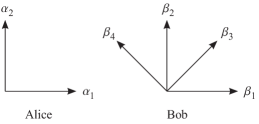
Figure 3.1: Settings in the BBM–CHSH protocol. Alice chooses between two orthogonal measurement directions $\alpha_{1}$ and $\alpha_{2}$, whereas Bob has four different possibilities, namely the same directions as Alice, i.e., $\beta_{1}$ and $\beta_{2}$, as well as two directions rotated by $\frac{\pi}{4}$, i.e. $\beta_{3}$ and $\beta_{4}$.

Leaking labs

The violation of a Bell inequality by the legitimate parties was found to be a necessary and sufficient condition for the efficient extraction of a quantum secret key as described in the previous section. We show that this link disappears as soon as one takes into account that some information can leak out of the laboratories of Alice and Bob. However, if the amount of leaked information is known, one can adapt a new bound in the Bell inequality and recover security again.

Apart from its fundamental meaning, the freedom to choose between different measurement settings can be regarded as an important resource in quantum secret key distribution. In particular, if the freedom in choosing the settings by the legitimate partners is abandoned an eavesdropper can both simulate the violation of a Bell inequality and successfully eavesdrop, as recently shown by Hwang [90]. Effectively, one can assume that each measurement device chooses its setting according to a pseudo-random sequence that is installed in the device beforehand. Such a model of lack of freedom allows the eavesdropper to know the algorithm generating pseudo-random numbers, at least to some extent, and correspondingly predict the future measurement settings.

In what follows we will consider the BBM-CHSH protocol and analyze both the violation of the CHSH inequality and the security of the key distribution as a function of the amount of knowledge that the eavesdropper Eve (E) has about the settings chosen by the legitimate parties Alice (A) and Bob (B).

Consider a source that emits pairs of spin-$\frac{1}{2}$ particles in the singlet state $|\psi^{-}\rangle=(|z+\rangle_{1}|z-\rangle_{2}-|z-\rangle_{1}|z+\rangle_{2})/\sqrt{2}$, where $|z+\rangle$ and $|z-\rangle$ denote spin-up and spin-down along the $z$ direction, respectively. The legitimate parties measure the incoming particles in the $xy$ plane. Alice can choose between two orthogonal settings, characterized by the azimuthal angles $\alpha_{1}\equiv 0$ and $\alpha_{2}\equiv\frac{\pi}{2}$, whereas Bob has four possible measurement directions, namely $\beta_{1}\equiv\alpha_{1}\equiv 0$, $\beta_{2}\equiv\alpha_{2}\equiv\frac{\pi}{2}$, $\beta_{3}\equiv\frac{\pi}{4}$, and $\beta_{4}\equiv\frac{3\pi}{4}$ (note that the $\beta_{j}$ are not numbered in ascending order). Therefore, depending on their choice of settings, they sometimes measure correlations for determining the violation of the CHSH inequality, namely with the four settings $(\alpha_{1},\beta_{3})$, $(\alpha_{1},\beta_{4})$, $(\alpha_{2},\beta_{3})$, and $(\alpha_{2},\beta_{4})$, or they can establish a key, since their outcomes are perfectly anti-correlated for measurements along $(\alpha_{1},\beta_{1})$ and $(\alpha_{2},\beta_{2})$. If they choose $(\alpha_{1},\beta_{2})$ or $(\alpha_{2},\beta_{1})$, i.e. orthogonal directions, they discard their results. A schematic of the measurement directions is shown in Fig. 3.1.

Let $P(X\!=\!-Y|ij)$ denote the probability that Alice and Bob obtain anti-correlated results if they measure along $\alpha_{i}$ and $\beta_{j}$, respectively, where $i=1,2$ and $j=1,2,3,4$. The (measured) CHSH expression has the form

$$S\equiv P(X\!=\!-Y|13)+P(X\!=\!-Y|23)+P(X\!=\!-Y|24)-P(X\!=\!-Y|14)\leq 2\,.$$ (3.12)

For the (maximally entangled) singlet state it is equal to $1+\sqrt{2}$. The classical bound is 2, whereas the logical bound is equal to 3.

Let us now assume that an eavesdropper has some knowledge about the choice of settings of Alice and Bob, for instance by having some insight into their random number generators. We model this knowledge in the following way: In each run, i.e., for each singlet pair, Eve knows that the combination of local settings $(\alpha_{i},\beta_{j})$ will happen with probability $q_{ij}$. For simplicity we assume that one out of the 8 joint settings will happen with (high) probability $Q\geq\tfrac{1}{8}$, whereas all the other 7 have equal (low) probability $\frac{1-Q}{7}$ to be manifested. The number $Q$ shall be the same for all runs; the setting which it indicates to be most probable of course changes from run to run. The case $Q=1$ corresponds to perfect knowledge of the eavesdropper and to the complete lack of free will of Alice and Bob, whereas $Q=\tfrac{1}{8}$ means that Eve has no knowledge at all.

We impose the following attack algorithm: If Eve believes one of the CHSH settings to be most likely, she sends the corresponding optimal product state. In general, if $q_{ij}=Q$, which means that the setting $(\alpha_{i},\beta_{j})$ is most probable from Eve’s viewpoint, she intercepts and sends either $\left|\alpha_{i}\right\rangle_{\text{A}}\left|\beta_{j}+\pi\right\rangle_{\text{B}}$ or $\left|\alpha_{i}+\pi\right\rangle_{\text{A}}\left|\beta_{j}\right\rangle_{\text{B}}$ (by tossing a fair coin, such that the local results of Alice and Bob are always totally random). Only in the special case $q_{14}=Q$, Eve sends $\left|\alpha_{1}\right\rangle_{\text{A}}\left|\beta_{4}\right\rangle_{\text{B}}$ or $\left|\alpha_{1}+\pi\right\rangle_{\text{A}}\left|\beta_{4}+\pi\right\rangle_{\text{B}}$. This is the CHSH setting where the probability of anti-correlation should be minimized, since $P(X\!=\!-Y|14)$ appears with a minus sign in the CHSH inequality. Therefore, she attacks the CHSH measurements in order to achieve a maximal violation ($S=3$) and the key establishing measurements to find the key (or rather produce it herself).

To further motivate the choice of this attack algorithm note that (i) it is canonical in the way that Eve attacks all events in the same way, namely with the appropriate product state. (ii) The attack is already good enough to show that the connection between violation of local realism and secure key distribution is lost in the case in which the eavesdropper has partial knowledge about the settings. (iii) Eve sends a product state for each pair that is generated by the source. Hence, Alice and Bob are faced with measurement results that can be described by local realism but nevertheless can violate the CHSH inequality (3.12) due to restricted freedom.

According to Eve’s setting knowledge and the attack strategy, one can compute the value for the CHSH expression as measured by Alice and Bob. In the subensemble of cases in which, e.g. Alice measures along $\alpha_{1}$ and Bob along $\beta_{3}$, Eve sends with probability $Q$ the product states resulting in anti-correlations $P(X\!=\!-Y|13)=1$. In the rest of the cases she sends 7 possible ”wrong guesses” which each happen with probability $\frac{1-Q}{7}$ and for each of them the probability for anti-correlations takes values between $\frac{1}{2}$ and $\cos^{2}\frac{\pi}{8}\approx 0.854$, depending on the specific wrong attack. The measured probability $P(X\!=\!-Y|13)$ is the expectation value of all 8 sets of anti-correlated results weighted with their probabilities to happen. Analogously, the other probabilities for anti-correlation are calculated and we find:

$$P(X\! =\!-Y|13)=Q+\tfrac{1-Q}{7}\left(\tfrac{5}{2}+2\,\cos^{2}\tfrac{\pi}{8}\right)\!,$$ (3.13)

$$P(X\! =\!-Y|23)=P(X\!=\!-Y|13)\,,$$ (3.14)

$$P(X\! =\!-Y|24)=Q+\tfrac{1-Q}{7}\left(\tfrac{5}{2}+\cos^{2}\tfrac{\pi}{8}+\sin^{2}\tfrac{\pi}{8}\right)\!,$$ (3.15)

$$P(X\! =\!-Y|14)=\tfrac{1-Q}{7}\left(\tfrac{5}{2}+\cos^{2}\tfrac{\pi}{8}+\sin^{2}\tfrac{\pi}{8}\right)\!.$$ (3.16)

The CHSH expression finally results in:

$$S=3\,Q+\tfrac{1-Q}{7}\left(5+4\,\cos^{2}\tfrac{\pi}{8}\right)\approx 1.2+1.8\,Q\,.$$ (3.17)

Thus, the logical bound $S_{\text{log}}\equiv 3$ is reached in the limit $Q\rightarrow 1$. The classical bound of $S_{\text{cl}}\equiv 2$ is beaten for all $Q>Q_{\text{cl}}\approx 0.44$ and the quantum mechanics (Cirel’son) bound $S_{\text{qm}}\equiv 1+\sqrt{2}\approx 2.41$ is beaten for setting knowledge $Q>Q_{\text{qm}}\approx 0.67$. If $Q$ is larger than $Q_{\text{qm}}$, Eve should reduce the strength of her attack, e.g. by mixing some noise into her product states, for otherwise even the quantum bound would be broken. The CHSH expression (3.17) and the bounds are shown in the left panel of Fig. 3.2.

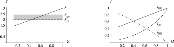
Figure 3.2: Left: The (measured) CHSH expression $S$ as a function of Eve’s setting knowledge $Q$ (solid line). The CHSH inequality with classical bound $S_{\text{cl}}=2$ (dotted line) is violated for every setting knowledge $Q>Q_{\text{cl}}\approx 0.44$. The quantum bound $S_{\text{qm}}=1+\sqrt{2}$ is also indicated. Right: The mutual information between Alice and Bob $I_{\text{AB}}$ (dashed line) and the actual mutual information between Bob and Eve $I_{\text{BE}}$ (solid line), which is always smaller than (or equal to) the Alice–Eve mutual information. For every setting knowledge $Q$ one has $I_{\text{BE}}\geq I_{\text{AB}}$ and thus Alice and Bob can never extract a secret key. An optimal attack without setting knowledge leads to $\tilde{I}_{\text{BE}}$ (dotted line). Only for $Q\leq Q_{0}\approx 0.63$ the BBM–CHSH protocol is secure, because Alice and Bob find $I_{\text{AB}}\leq\tilde{I}_{\text{BE}}$ and they will not use their key.

When is Eve’s knowledge about the settings also sufficient to find out the key which is established by Alice and Bob? To answer this question, we have to compute mutual informations between the parties. The mutual information between Alice and Bob is determined by the bit error rate [83] which they can compute in the subensembles where they measured along $\alpha_{1}\!=\!\beta_{1}\!=\!0$ or $\alpha_{2}\!=\!\beta_{2}\!=\!\frac{\pi}{2}$. Let us consider the first; the error rate in the second is the same for symmetry reasons. The bit error rate $D$ is given by the sum of 8 terms corresponding to the 8 settings that were potentially possible from Eve’s point of view. Each term is the probability with which Eve believed this event would happen — $Q$ for the event $(\alpha_{1},\beta_{1})$ itself and $\frac{1-Q}{7}$ for all the others (the wrong guesses), corresponding to our definition of the setting knowledge — multiplied with the probability that the attack $(\alpha_{i},\beta_{j})$ leads to a correlation (error) rather than an anti-correlation as for the original singlet state. This ”destruction probability” is $0$ for the ”correct” event $(\alpha_{1},\beta_{1})$. It is $\sin^{2}\frac{\pi}{8}$ for both $(\alpha_{1},\beta_{3})$ and $(\alpha_{1},\beta_{4})$, and $\frac{1}{2}$ for all the others (where an orthogonal state was sent to Alice or Bob). Finally, we find the bit error rate

$$D=\tfrac{1-Q}{7}\left(\tfrac{5}{2}+2\,\sin^{2}\tfrac{\pi}{8}\right)\approx 0.4\,(1-Q)\,.$$ (3.18)

The mutual information between Alice and Bob reads [83]:

$$I_{\text{AB}}\equiv 1-H(D)\,,$$ (3.19)

The maximal mutual information between Alice (or Bob for symmetry reasons) and Eve from Alice’s and Bob’s viewpoint, which can be attained by an optimal attack of Eve for a given error rate $D$ and under the condition that Eve has no setting knowledge is given by [83]:

$$\tilde{I}_{\text{AE}}=\tilde{I}_{\text{BE}}=1-H(\tfrac{1}{2}\!+\!\sqrt{D-D^{2}})\,.$$ (3.20)

The actual mutual information between Alice and Eve, $I_{\text{AE}}$, can be computed from the conditional entropy $H(A|E)$ by $I_{\text{AE}}=H(A)-H(A|E)$. Since the outcomes of Alice are locally random for all possible attacks the Shannon information of Alice is $H(A)=1$. As all chosen settings are publicly revealed after the measurements, Eve can compute $H(A|E)$ in the subensemble of the key establishing measurement $(\alpha_{1},\beta_{1})$. (If Alice and Bob measure along $(\alpha_{2},\beta_{2})$, the result does not change.) The calculation itself is straightforward, once one realizes that $H(A|e)=0$ for all 4 events $e$ in which Eve (justly) believed that Alice would choose $\alpha_{1}$, as Eve knows her result in this case. If Eve made the (wrong) guess $\alpha_{2}$ then $H(A|e)=1$ for these 4 possible events, for Alice measures in the orthogonal direction $\alpha_{1}$. Thus, $H(A|E)=4\,\frac{1-Q}{7}$ and

$$I_{\text{AE}}=1-4\,\tfrac{1-Q}{7}=\tfrac{3}{7}+\tfrac{4}{7}\,Q\,.$$ (3.21)

Analogously, one can find the actual mutual information between Bob and Eve:

$$I_{\text{BE}}=1-\tfrac{1-Q}{7}\left(2+4\,H(\cos^{2}\tfrac{\pi}{8})\right)\approx 0.37+0.63\,Q\,,$$ (3.22)

which is always smaller than (or equal to) $I_{\text{AE}}$. We have

$$I_{\text{AB}}\leq I_{\text{BE}}$$ (3.23)

for all $Q$ and equality only holds for $Q=1$. Alice and Bob can never extract a secret key, since the condition $I_{\text{AB}}>I_{\text{AE}}$ is never fulfilled (right panel of Fig. 3.2).

If Eve has no setting knowledge the quantum protocol is secure if and only if quantum bit error rate is below $D<D_{0}=\tfrac{1}{2}\,(1-\tfrac{1}{\sqrt{2}})\approx 0.15$, which in turn is equivalent to $S>2$ [83]. In the present case the critical error rate $D_{0}$ corresponds, according to (3.18), to a setting knowledge $Q_{0}\approx 0.63$. For this knowledge $I_{\text{AB}}=\tilde{I}_{\text{BE}}$. If $Q>Q_{0}$, the BBM–CHSH protocol is insecure, since $I_{\text{AB}}\leq I_{\text{BE}}$ and Alice and Bob find both their error rate to be sufficiently small (below $D_{0}$) and the CHSH inequality (3.12) to be violated, which makes them think they are safe. In fact, for the CHSH expression not to exceed the quantum value the setting knowledge should be below $Q_{\text{qm}}\approx 0.67$. For $Q\leq Q_{0}$ Eve’s setting knowledge is ”insufficient” and the protocol becomes secure: Alice and Bob cannot extract a secret key because still $I_{\text{AB}}<I_{\text{BE}}$, but they find $I_{\text{AB}}\leq\tilde{I}_{\text{BE}}$ and know that there might be an eavesdropper and thus they will not use the key. For $0.44\approx Q_{\text{cl}}<Q\leq Q_{0}\approx 0.63$ Alice and Bob find the CHSH inequality (3.12) to be violated ($S>2$) and nonetheless they cannot extract a secret key ($I_{\text{AB}}\leq\tilde{I}_{\text{BE}}$, $D\geq D_{0}$). Therefore, we deduce that the equivalence between the violation of Bell’s inequality (with complete freedom) and the secure key distribution (without freedom) is lost.

If Alice and Bob knew $Q$, which means they knew to which extent their freedom is restricted, and if they calculated the maximal $\Delta_{\text{CHSH}}$ under the constraint of an insecure key, $I_{\text{AB}}\leq\min\{I_{\text{AE}},I_{\text{BE}}\}$, for all possible attacks, then a violation of the CHSH inequality with the new bound $2+\Delta_{\text{CHSH}}$ would be equivalent to the possibility of efficient secret key extraction (unless the new bound is larger than $S_{\text{qm}}=1+\sqrt{2}$). A violation of this new bound is equivalent to statement that the classical bound 2 is violated in the case of total freedom and for this situation there exists a complete equivalence between the CHSH inequality violation and the security of the BBM protocol [26, 71].

To conclude, if some information leaks out of the authorized parties’ laboratories the violation of the standard CHSH inequality is not equivalent to a secure key distribution. Nevertheless, one can define a new (higher) bound whose violation indeed guarantees the security of the key. Therefore, one can keep the security while, to some extent, relaxing the assumption that no information about the measurement settings is revealed to an eavesdropper, as long as the amount of this information is known.

3.3 Qudit quantum cryptography with composite systems [P2]

Quantum cryptography as just described uses two-level quantum systems. If higher-dimensional systems (qudits) are at disposal one can increase the security of the quantum protocol, i.e. the level of allowed errors can be bigger [24, 91, 92]. The question to be answered in this section is whether such cryptosystems are feasible. It will be shown that two-bases quantum cryptography with qudits composed of two lower-dimensional subsystems can be realized with individual measurements on subsystems accompanied with classical communication. We will use the description of a $d$-level system in terms of unitary generalizations of Pauli operators: $S_{kl}=S_{x}^{k}S_{z}^{l}$ with $k,l=0,...,d-1$ (Appendix B).

Generally, an arbitrary measurement can be viewed as a unitary evolution of the system which transforms the eigenvectors of the observable into the eigenvectors which can be distinguished by the measurement apparatus. Thus, we solve the eigenproblem of the generalized Pauli operators, and next apply it to the measurements of quantum cryptography.

3.3.1 Eigenproblem of the generalized Pauli operators

The matrix of any $S_{kl}$ operator, written in the $S_{z}$ basis $|\kappa\rangle_{z}$, has only $d$ non-vanishing entries, one per column and row:

$$S_{kl}=\left(\begin{array}[]{ccccccc}0&0&&0&\alpha_{d}^{(d-k)l}&&0\\ \vdots&\vdots&&\vdots&\vdots&&\vdots\\ 0&0&&0&0&&\alpha_{d}^{(d-1)l}\\ 1&0&\ldots&0&0&\ldots&0\\ 0&\alpha_{d}^{l}&&0&0&&0\\ \vdots&\vdots&&\vdots&\vdots&&\vdots\\ 0&0&&\alpha_{d}^{(d-k-1)l}&0&&0\end{array}\right).$$

The only non-vanishing element of the first column, a “1”, appears in the $k$th row (recall that $k=0,1,...,d-1$). Generally, the matrix elements of the $S_{kl}$ operator, $[S_{kl}]_{rm}$, are given by $[S_{kl}]_{rm}=\delta_{r-k,m}\alpha_{d}^{ml}$, where $\delta_{x,y}$ is the Kronecker delta. Since every $S_{kl}$ is unitary it can be diagonalized:

$$S_{kl}=VDV^{\dagger},$$ (3.24)

where $V$ is a unitary matrix the columns of which are eigenstates of $S_{kl}$, $V=(|0\rangle,...,|d-1\rangle)$, and $D$ is a diagonal matrix with entries being eigenvalues of $S_{kl}$, denoted by $\lambda_{j}$. The form of $[S_{kl}]_{rm}$ and (3.24) imply conditions, which must be satisfied by the eigenvectors $|j\rangle$:

$$\sum_{j=0}^{d-1}\lambda_{j}v_{k+m,j}v_{m,j}^{*}=\alpha_{d}^{ml},\quad\textrm{for all}\quad m=0,...,d-1,$$ (3.25)

where $v_{i,j}$ is the element of the matrix $V$ in the $i$th row and $j$th column, i.e. $i$th coefficient of the eigenvector $|j\rangle$. A study of this condition allows one to construct the eigenbasis.

We first present the result, that is give a candidate for an eigenbasis, and then prove that this is indeed the eigenbasis. Depending on $k$ the eigenstates of $S_{kl}$ are given by superposition of different number of states $|\kappa\rangle_{z}$. Let us denote by $f$ the smallest multiple of $k$ modulo $d$, i.e. $f=\min_{x=1,2,...}[kx]_{d}$. The values of $f$ are taken to be strictly positive, i.e. $f=1,2,...$. Within this definition $k=wf$ is a multiple of $f$. Eigenstates $|j\rangle$ involve every $f$th state of the $S_{z}$ basis:

$$|\kappa\rangle_{z}=|a+\eta^{\prime}f\rangle_{z}=|a+\eta k\rangle_{z},$$ (3.26)

where $\eta^{\prime}=0,...,d/f-1$ and $a=0,...,f-1$, and of course $\eta^{\prime}=w\eta$. Both $\eta^{\prime}$ and $\eta$ enumerate different states $|\kappa\rangle_{z}$ into which $|j\rangle$ is decomposed, i.e. $\eta=0,...,d/f-1$. All other coefficients vanish. The whole eigenbasis splits into $f$ groups of eigenvectors which are superposition of vectors $|\kappa\rangle_{z}$ with fixed $a$. There are $d/f$ eigenvectors within each group. To uniquely identify the eigenvector $|j\rangle$ one needs to specify $a$, and additionally an integer $g=0,...,d/f-1$, i.e. $j=j_{g,a}$. With these definitions we can present the form of eigenvectors (a candidate):

$$|j\rangle=|j_{g,a}\rangle=\sum_{\eta=0}^{d/f-1}v_{\eta k,j_{g,a}}|a+\eta k\rangle_{z},$$ (3.27)

with

$$v_{\eta k,j_{g,a}}=\frac{1}{\sqrt{d/f}}\lambda_{j_{g,0}}^{-\eta}\alpha_{d}^{\frac{\eta(\eta-1)}{2}kl},$$ (3.28)

where generally the eigenvalues $\lambda_{j_{g,a}}$ are given by:

$$\lambda_{j_{g,a}}=e^{i\varphi}\alpha_{d}^{gf+al},$$ (3.29)

and $e^{i\varphi}$ is a phase factor common to all the eigenvalues. We will show below how to compute this phase. Note that the coefficients (3.28) are independent of $a$. This can be intuitively explained by noting that for different $a$’s the eigenvectors $|j_{g,a}\rangle$ are orthogonal just due to the fact that they involve orthogonal vectors $|a+\eta k\rangle_{z}$. For a fixed $a$, but different $g$’s, the vectors (3.27) with coefficients (3.28) are also orthogonal. Their scalar product $\langle j_{g^{\prime},a}|j_{g,a}\rangle=(d/f)^{-1}\sum_{\eta=0}^{d/f-1}(\lambda_{j_{g^{\prime},0}}\lambda_{j_{g,0}}^{-1})^{\eta}$ involves the product of $\lambda_{j_{g^{\prime},0}}\lambda_{j_{g,0}}^{-1}=\alpha_{d}^{(g^{\prime}-g)f}=\alpha_{d/f}^{(g^{\prime}-g)}$, and the whole sum is equal to the Kronecker delta $\delta_{g^{\prime},g}$. Thus, the vectors $|j_{g,a}\rangle$ form an orthonormal basis.

To prove that this basis is the eigenbasis one needs to check whether

$$S_{kl}|j_{g,a}\rangle=\lambda_{j_{g,a}}|j_{g,a}\rangle.$$ (3.30)

The action of $S_{kl}$, defined in the Appendix B by (5.39), on the state $|j_{g,a}\rangle$ is given by:

$$S_{kl}|j_{g,a}\rangle=\frac{1}{\sqrt{d/f}}\sum_{\eta=0}^{d/f-1}\lambda_{j_{g,0}}^{-\eta}\alpha_{d}^{\frac{\eta(\eta-1)}{2}kl}\alpha_{d}^{l(a+\eta k)}|a+(\eta+1)k\rangle_{z},$$

Changing the summation index to $\eta_{1}=\eta+1$ one finds:

$$S_{kl}|j_{g,a}\rangle=\lambda_{j_{g,0}}\alpha_{d}^{al}\frac{1}{\sqrt{d/f}}\sum_{\eta_{1}=1}^{d/f}\lambda_{j_{g,0}}^{-\eta_{1}}\alpha_{d}^{\frac{\eta_{1}(\eta_{1}-1)}{2}kl}|a+\eta_{1}k\rangle_{z}.$$ (3.31)

The coefficients within the sum are equal to the coefficients of the initial $|j_{g,a}\rangle$ state, (3.28), if for the last term in (3.31), for which $\eta_{1}=d/f$, one has:

$$\lambda_{j_{g,0}}^{-d/f}=\alpha_{d}^{-\frac{1}{2}\frac{d}{f}(\frac{d}{f}-1)kl}.$$ (3.32)

This equation gives the eigenvalues $\lambda_{j_{g,0}}$. If one takes one of the solutions to (3.32), say $\lambda_{j_{0,0}}$, in the form $\lambda_{j_{0,0}}=e^{i\varphi}$, then the remaining solutions are given by $\lambda_{j_{g,0}}=e^{i\varphi}\alpha_{d/f}^{g}$. Indeed, if $\lambda_{j_{0,0}}$ satisfies (3.32), then also $\lambda_{j_{g,0}}$ satisfy it. The eigenvalues for other $a$’s are given by:

$$\lambda_{j_{g,a}}=\lambda_{j_{g,0}}\alpha_{d}^{al}.$$ (3.33)

Note that degeneracies in the eigenproblem can only appear for $f\neq 1$ (since for $f=1$ one has only $a=0$, and $g$ takes all $d$ different values).

Practically, to compute the eigenvectors one should find the value of $f$. If it is different than unity, set $a=0$ and compute the coefficients according to Eq. (3.28). For other values of $a$ the coefficients are the same, but now they are multiplied with orthogonal vectors $|a+\eta k\rangle_{z}$. To compute the eigenvalues one needs to solve Eq. (3.32). Moreover, once $\lambda_{j_{g,0}}$ has been found for some $g$ the other eigenvalues for $a=0$ are obtained by multiplication of $\alpha_{d/f}$: $\lambda_{j_{g^{\prime},0}}=\lambda_{j_{g,0}}\alpha_{d/f}^{g^{\prime}-g}$. The eigenvalues for $a\neq 0$ can be found from (3.33).

Example. Take $S_{43}$ for $d=6$, i.e. $k=4,l=3$ and one finds $f=2$. Put $a=0$. From (3.32) one has $\lambda_{j_{g,0}}=e^{ig\frac{2\pi}{3}}=\alpha_{6}^{2g}=\alpha_{3}^{g}$ ($e^{i\varphi}=1$). According to (3.33), the eigenvalues $\lambda_{j_{g,1}}$ are equal to $\lambda_{j_{g,1}}=-\lambda_{j_{g,0}}$. This can be summarized in the eigenbasis:

$$\begin{array}[]{lcl}|0\rangle=\frac{1}{\sqrt{3}}\Big{(}|0\rangle_{z}+|2\rangle_{z}+|4\rangle_{z}\Big{)},&&|1\rangle=\frac{1}{\sqrt{3}}\Big{(}|1\rangle_{z}+\alpha_{3}^{2}|3\rangle_{z}+\alpha_{3}|5\rangle_{z}\Big{)},\\ |2\rangle=\frac{1}{\sqrt{3}}\Big{(}|0\rangle_{z}+\alpha_{3}|2\rangle_{z}+\alpha_{3}^{2}|4\rangle_{z}\Big{)},&&|3\rangle=\frac{1}{\sqrt{3}}\Big{(}|1\rangle_{z}+|3\rangle_{z}+|5\rangle_{z}\Big{)},\\ |4\rangle=\frac{1}{\sqrt{3}}\Big{(}|0\rangle_{z}+\alpha_{3}^{2}|2\rangle_{z}+\alpha_{3}|4\rangle_{z}\Big{)},&&|5\rangle=\frac{1}{\sqrt{3}}\Big{(}|1\rangle_{z}+\alpha_{3}|3\rangle_{z}+\alpha_{3}^{2}|5\rangle_{z}\Big{)}.\end{array}$$

3.3.2 Cryptography

Consider the two-bases quantum cryptography protocol with $d$-level systems, as described in [24]. One has a qudit randomly prepared in a state of a certain basis, or of another basis, which is unbiased with respect to the first one, i.e. every state form the first basis has equal overlap with all the states of another basis [93, 94]. The measurement basis is also randomly chosen between these two. The two mutually unbiased bases can be chosen as the eigenbases of the $S_{z}$ and $S_{x}$ generalized Pauli operators. Applying relation (3.28) to $S_{x}=S_{10}$ one finds, for arbitrary dimension, the well-known Fourier relation between the $S_{z}$ and $S_{x}$ eigenbases:

$$|j\rangle_{x}=\frac{1}{\sqrt{d}}\sum_{\kappa=0}^{d-1}\alpha_{d}^{-\kappa j}|\kappa\rangle_{z},$$ (3.34)

i.e. $|_{x}\langle j|\kappa\rangle_{z}|=1/\sqrt{d}$ for all $j$ and $\kappa$ (indeed the bases are mutually unbiased).

Consider a $d$-level system encoded in two subsystems. Let us define the eigenbasis of a global $S_{z}$ operator as:

$$|\kappa\rangle_{z}=|d_{0}\kappa_{1}+\kappa_{0}\rangle_{z}\equiv|\kappa_{1}\rangle_{1}|\kappa_{0}\rangle_{0},$$ (3.35)

where $\kappa_{i}=0,...,d_{i}-1$, and $|\kappa_{0}\rangle_{0}$, $|\kappa_{1}\rangle_{1}$ denote the states of subsystems “0” and “1”, respectively. Within this definition a measurement of the global observable $S_{z}$ is equivalent to individual measurements on the components. These individual measurements reveal the values of $\kappa_{0}$ and $\kappa_{1}$, and the eigenvalue of $S_{z}$ is $\alpha_{d}^{d_{0}\kappa_{1}+\kappa_{0}}$.

To measure $S_{x}$ one uses the definition (3.35) and the fact that the dimension of a global system, $d$, is the product of dimensions of subsystems, $d=d_{1}d_{0}$, and finds that:

$$|j\rangle_{x}=\frac{1}{\sqrt{d_{1}}}\sum_{\kappa_{1}=0}^{d_{1}-1}\alpha_{d}^{-d_{0}\kappa_{1}j}|\kappa_{1}\rangle_{1}\otimes\frac{1}{\sqrt{d_{0}}}\sum_{\kappa_{0}=0}^{d_{0}-1}\alpha_{d}^{-\kappa_{0}j}|\kappa_{0}\rangle_{0},$$ (3.36)

where we have used the symbol $\otimes$ to stress the factorization of this state. For $j=j_{1}+d_{1}j_{0}$ the state of subsystem “1” reads:

$$\frac{1}{\sqrt{d_{1}}}\sum_{\kappa_{1}=0}^{d_{1}-1}\alpha_{d}^{-d_{0}\kappa_{1}j_{1}-d_{0}\kappa_{1}d_{1}j_{0}}|\kappa_{1}\rangle_{1}.$$ (3.37)

Since $\alpha_{d}^{d_{0}}=\alpha_{d_{1}}$, see (5.40), and $e^{-i2\pi\kappa_{1}j_{0}}=1$ a measurement on this subsystem in the basis

$$|\phi_{j_{1}}\rangle_{1}=\frac{1}{\sqrt{d_{1}}}\sum_{\kappa_{1}=0}^{d_{1}-1}\alpha_{d_{1}}^{-\kappa_{1}j_{1}}|\kappa_{1}\rangle_{1}$$ (3.38)

reveals the value of $j_{1}$. The value of $j_{0}$ can be measured once $j_{1}$ is known. A measurement in the basis

$$|\psi_{j_{0}}\rangle_{0}=\frac{1}{\sqrt{d_{0}}}\sum_{\kappa_{0}=0}^{d_{0}-1}\alpha_{d}^{-(j_{1}+d_{1}j_{0})\kappa_{0}}|\kappa_{0}\rangle_{0}$$ (3.39)

on the subsystem “0” reveals the value of $j_{0}$. In this way all values of $j$ can be measured using individual measurements and classical communication. Since the measurement on subsystem “0” depends on the outcome of the measurement on subsystem “1”, the (classical) information about the outcome needs to be fed-forward to the device measuring subsystem “0”.

3.4 Quantum communication complexity

In a communication complexity problem (CCP) [95], separated parties performing local computations exchange information in order to accomplish a globally defined task, which is impossible to solve singlehandedly. Two types of CCPs can be distinguished: in the first type one asks for a minimal amount of information exchange necessary to solve a task with certainty [96, 97, 98]; in the second type one maximizes the probability of successfully solving a task with a restricted amount of communication [23, 98, 99, 100]. Such studies aim, e.g., at a speedup of a distributed computation of very large scale integrated circuits and data structures [101].

Communication complexity was introduced in 1979 by Yao [95], who was also the first to introduce the quantum version. However, only recently it was noticed that the problems are ultimately linked with violation of local realism. It was shown that one can link a CCP with every Bell inequality for qubits [23]. Quantum protocols for the CCPs, utilizing entangled states which violate the inequalities, outperform the best classical protocol [25].

Interestingly, it is possible to recast some entanglement-based CCPs in terms of a single qubit sequentially transmitted between the participants [102]. Also in this case the limits of performance of classical protocols are described by a form of “Bell inequality” [25]. This type of communication complexity was experimentally realized in the group of Weinfurter [25].

In this section we follow the general link between violation of Bell inequality and CCPs [23] for the case of the inequality with an arbitrary number of settings [P3]. Next, we give quantum communication complexity protocols using higher-dimensional entangled systems [P7] that are linked with the Bell inequality for multilevel systems [103].

3.4.1 Qubits [P3]

Let us focus on a variant of a CCP, in which each of $N$ separated partners receives arguments, $y_{n}=\pm 1$ and $x_{n}=0,...,M-1$, of some globally defined function, $\mathcal{F}\equiv\mathcal{F}(y_{1},x_{1},...,y_{N},x_{N})$. The inputs of the $n$th party are not known to any other party. Assume the bits $y_{n}$ are randomly distributed, and inputs $x_{n}$ (representing $\textrm{lg}M$ bits of information) can in general be distributed according to a weight $\mathcal{W}(x_{1},...,x_{2})$. The goal is to maximize the probability that Alice arrives at the correct value of the function, under the restriction of $N-1$ bits of overall communication. Before participants receive their inputs they are allowed to do anything from which they can derive benefit. In particular, they can share some correlated strings of numbers in the classical scenario or entangled states in the quantum case.

The problem. Following [23] one chooses for a task-function:

$$\mathcal{F} = y_{1}...y_{N}{\rm Sign}[\cos(\phi_{x_{1}}^{1}+...+\phi_{x_{N}}^{N})]=\pm 1,$$ (3.40)

with the angles defined by (2.101). Additionally, the $x_{n}$ inputs are distributed with the weight

$$\mathcal{W}(x_{1},...,x_{2})=(1/\mathcal{N})|\cos(\phi_{x_{1}}^{1}+...+\phi_{x_{N}}^{N})|,$$ (3.41)

with the normalization factor $\mathcal{N}=\sum_{x_{1}...x_{N}=0}^{M-1}|\cos(\phi_{x_{1}}^{1}+...+\phi_{x_{N}}^{N})|$. After the communication takes place, if Alice misses some of the random variables $y_{n}$, her “answer” can only be random. Thus, in an optimal protocol each party must communicate one bit. Essentially, there are two communication structures which lead to a non-random answer: (i) each party transmits one bit directly to Alice, and (ii) sequence of a peer-to-peer exchanges with Alice at the end. The task is to maximize the probability of correct answer $\mathcal{A}\equiv\mathcal{A}(y_{1},x_{1},...,y_{N},x_{N})$. Since both $\mathcal{A}$ and $\mathcal{F}$ are dichotomic variables this amounts in maximizing:

$$P_{{\rm correct}}=\frac{1}{2^{N}}\sum_{{\bf y},{\bf x}}\mathcal{W}(x_{1},...,x_{2})P_{{\bf y},{\bf x}}(\mathcal{A}\mathcal{F}=1),$$ (3.42)

where $\frac{1}{2^{N}}$ describes (random) distribution of $y_{n}$’s, and $P_{{\bf y},{\bf x}}(\mathcal{A}\mathcal{F}=1)$ is a probability that $\mathcal{A}=\mathcal{F}$ for given inputs ${\bf y}\equiv(y_{1},...,y_{N})$ and ${\bf x}=(x_{1},...,x_{N})$. It is useful to express the last probability in terms of an average value (over many runs of the protocol) of a product $\langle\mathcal{A}\mathcal{F}\rangle_{{\bf y},{\bf x}}$:

$$P_{{\bf y},{\bf x}}(\mathcal{A}\mathcal{F}=1)=\frac{1}{2}\Big{[}1+\langle\mathcal{A}\mathcal{F}\rangle_{{\bf y},{\bf x}}\Big{]}.$$ (3.43)

Since $\mathcal{F}$ is independent of $\mathcal{A}$, and for given inputs it is constant, one has $\langle\mathcal{A}\mathcal{F}\rangle_{{\bf y},{\bf x}}=\mathcal{F}\langle\mathcal{A}\rangle_{{\bf y},{\bf x}}$. Finally the probability of a correct answer reads $P_{{\rm correct}}=\frac{1}{2}[1+(\mathcal{F},\mathcal{A})]$, and it is in one-to-one correspondence with a “weighted” scalar product (average success):

$$(\mathcal{F},\mathcal{A})=\frac{1}{2^{N}}\sum_{{\bf y},{\bf x}}\mathcal{W}(x_{1},...,x_{2})\mathcal{F}\langle\mathcal{A}\rangle_{{\bf y},{\bf x}}.$$ (3.44)

Using the definitions (3.41) for $\mathcal{W}$ and (3.40) for $\mathcal{F}$ one gets:

$$(\mathcal{F},\mathcal{A})=\frac{1}{2^{N}}\frac{1}{\mathcal{N}}\sum_{{\bf y},{\bf x}}y_{1}...y_{N}\cos(\phi_{x_{1}}^{1}+...+\phi_{x_{N}}^{N})\langle\mathcal{A}\rangle_{{\bf y},{\bf x}},$$ (3.45)

with angles given by (2.101). We focus our attention on maximization of this quantity.

Classical scenario. In the best classical protocol each party locally computes a bit function $e_{n}=y_{n}f(x_{n},\lambda)$, with $f(x_{n},\lambda)=\pm 1$, where $\lambda$ denotes some previously shared classical resources. Next, the bit is sent to Alice, who puts as an answer the product $\mathcal{A}_{c}=y_{1}f(x_{1},\lambda)e_{2}...e_{N}=y_{1}...y_{N}f(x_{1},\lambda)...f(x_{N},\lambda)$. The same answer can be reached in the peer-to-peer strategy, simply the $n$th party sends $e_{n}=y_{n}f(x_{n},\lambda)e_{n-1}$. For the given inputs the procedure is always the same, i.e. $\langle\mathcal{A}_{c}\rangle_{{\bf y},{\bf x}}=\mathcal{A}_{c}$. To prove the optimality of this protocol, one follows the proof of [25], with the only difference that $x_{n}$ is a $M$-valued variable now. This, however, does not invalidate any of the steps of [25], and we will not repeat that proof.

Inserting the product form of $\mathcal{A}_{c}$ into the average success (3.45), using the fact that $y_{n}^{2}=1$, and summing over all $y_{n}$’s one obtains

$$(\mathcal{F},\mathcal{A}_{c})=\frac{1}{\mathcal{N}}\sum_{x_{1}...x_{N}=0}^{M-1}\!\!\!\!\!\cos(\phi_{x_{1}}^{1}+...+\phi_{x_{N}}^{N})f(x_{1},\lambda)...f(x_{N},\lambda),$$ (3.46)

which has the same structure as the local realistic expression (2.103). Thus, the highest classically achievable average success is given by a local realistic bound: $\max(\mathcal{F},\mathcal{A}_{c})=(1/\mathcal{N})B_{LR}(N,M)$.

Quantum scenario. In the quantum case participants share a $N$-party entangled state $\rho$ before delivery of the inputs. After receiving inputs each party measures the $x_{n}$th observable on the state, where the observables are enumerated as in the Bell inequality (2.112). This results in a measurement outcome, $f_{n}$. Each party sends $e_{n}=y_{n}f_{n}$ to Alice, who then puts as an answer the product $\mathcal{A}_{q}=y_{1}...y_{N}f_{1}...f_{N}$. For the given inputs the average answer reads $\langle\mathcal{A}_{q}\rangle_{{\bf y},{\bf x}}=y_{1}...y_{N}\langle f_{1}...f_{N}\rangle=y_{1}...y_{N}E_{x_{1}...x_{N}}^{\rho}$, and the maximal average success is given by a quantum value:

$$(\mathcal{F},\mathcal{A}_{q})=\frac{1}{\mathcal{N}}\sum_{x_{1}...x_{N}=0}^{M-1}\!\!\!\!\!\cos(\phi_{x_{1}}^{1}+...+\phi_{x_{N}}^{N})E_{x_{1}...x_{N}}^{\rho}.$$ (3.47)

The average advantage of quantum versus classical protocol can be quantified by $(\mathcal{F},\mathcal{A}_{q})/(\mathcal{F},\mathcal{A}_{c})$ which is equal to a violation factor, $V(N,M)$, introduced before in Eq. (2.128). Thus, all the states which violate the Bell inequality (including bound entangled states) are a useful resource for the communication complexity task. Optimally one should use the GHZ states $|\psi^{\pm}\rangle$, as they maximally violate the inequality.

Alternatively, one can compare the probabilities of success, $P_{\textrm{correct}}$, in the quantum and classical case. In Table 3.1 we gather the ratios between quantum and classical success probabilities for small number of participants. Clearly, one outperforms classical protocols for every $N$ and every $M$.

$N\backslash M$	2	3	4	5	$\infty$
2	1.1381	1.1196	1.1009	1.1002	1.0909
3	1.3333	1.2919	1.2815	1.2773	1.2709
4	1.3657	1.4395	1.4038	1.4258	1.4192
5	1.6000	1.5582	1.5467	1.5418	1.5336

Table 3.1: The ratio between probabilities of success in quantum and (optimal) classical protocol $P_{\textrm{correct}}^{qm}/P_{\textrm{correct}}^{cl}$ for the communication complexity problem with $N$ observers and $M$ settings. Quantum protocol uses GHZ state.

3.4.2 Qudits [P7]

In this section we present CCPs connected with Bell inequalities for higher-dimensional systems [103]. For a wide class of classical protocols we find an increase in the separation between the efficiency of the quantum and classical strategies, which grows with the dimensionality of the entangled systems. We show that the quantum protocol is more efficient than the classical ones if and only if the protocol participants share a state that violates the CGLMP inequalities for higher-dimensional systems [103]. The results form a generalization of those of [100] to arbitrarily high-dimensional systems.

The problem. Two parties are asked to give a single answer to $2\lfloor d/2\rfloor$ questions, where $\lfloor x\rfloor$ stands for the integer part of $x$. The integer $d$ describes the number of possible answers to each question. Each party locally receives two inputs, one bit and one dit, but is restricted to communicate only a dit to the other party. Further, the parties are not allowed to differ in their answers. That is, they must produce two identical answers each time.

Formally, the $2\lfloor d/2\rfloor$ questions will be formulated as a problem of computation of $\lfloor d/2\rfloor$ functions $f_{k}^{+}$ and $\lfloor d/2\rfloor$ functions $f_{k}^{-}$, with $k=0,...,\lfloor d/2\rfloor-1$. The parties give one answer to the question about the values of all $2\lfloor d/2\rfloor$ functions and their goal is to give the correct value of $\lfloor d/2\rfloor$ functions $f_{k}^{+}$, with the highest possible probability, and at the same time, the correct value of $\lfloor d/2\rfloor$ functions $f_{k}^{-}$ with the lowest possible probability. The questions are not treated equally. The importance of questions changes with the weight $1-\frac{2k}{d-1}$.

We now introduce the two-party task in detail and give all the functions explicitly: Alice receives a data string $\alpha=(a_{bit},a_{dit})$ and Bob a string $\beta=(b_{bit},b_{dit})$. Alice’s string is a combination of a bit $a_{bit}\in\{0,1\}$ and a dit $a_{dit}\in\{1,\alpha_{d},\alpha_{d}^{2},\dots,\alpha_{d}^{d-1}\}$ where $\alpha_{d}=e^{i(2\pi/d)}$. Similarly, Bob’s string is a combination of a bit $b_{bit}\in\{0,1\}$ and a dit $b_{dit}\in\{1,\alpha_{d},\alpha_{d}^{2},\dots,\alpha_{d}^{d-1}\}$. All possible input strings are distributed randomly. Before they give their answers, Alice and Bob are allowed to exchange two dits of information. The answers are in the form of one dit. The task of Alice and Bob is to maximize (having in mind the weight of the questions) all differences between the probabilities $P(f_{k}^{+})$, of giving the correct value for the functions

$$f^{+}_{k}=a_{dit}b_{dit}\alpha_{d}^{a_{bit}b_{bit}+k(-1)^{a_{bit}+b_{bit}}},\quad\textrm{ with}\quad k=0,\dots,\lfloor d/2\rfloor-1,$$ (3.48)

and $P(f_{k}^{-})$, of giving the correct value for the functions

$$f^{-}_{k}=a_{dit}b_{dit}\alpha_{d}^{a_{bit}b_{bit}+(k+1)(-1)^{a_{bit}+b_{bit}+1}},\quad\textrm{ with}\quad k=0,\dots,\lfloor d/2\rfloor-1.$$ (3.49)

That is, they aim at the maximal value of

$$\Delta=\sum_{k=0}^{\lfloor\frac{d}{2}\rfloor-1}\Big{(}1-\frac{2k}{d-1}\Big{)}\Big{(}P(f^{+}_{k})-P(f^{-}_{k})\Big{)}.$$ (3.50)

We will show that, if two parties use a class of classical protocols, the quantity $\Delta$ introduced above, which describes a performance of the protocol, is at most $\frac{1}{2}$, whereas if they use two entangled qudits $\Delta$ can be larger. Furthermore it increases with $d$.

Quantum versus classical protocol. Note that if only one of the independent inputs, $a_{dit}$ or $b_{dit}$, is random the product $a_{dit}b_{dit}$ in the full functions $f_{k}^{\pm}$ acquires completely random values. This is not the case for the last factors, with inputs $a_{bit}$ and $b_{bit}$. Thus, intuition suggests that a good classical protocol for the two parties may be that Alice “spends” her dit by sending $a_{dit}$ and Bob by sending $b_{dit}$ and that they put for the part of $f$’s dependent on the bits the value most often appearing in the third column and, at the same time, least often appearing in the fourth column of the Table 3.2. Moreover, because of the weight function they should give preference to the values connected with functions for $k=0$. The second factor of $f_{0}^{+}$ is equal to $1$ in three out of four cases, whereas $f_{0}^{-}$ is $1$ in one of four cases. Thus if each of them gives the value $a_{dit}b_{dit}$ as the answer, $\Delta=1(0.75-0.25)=0.5$.

$a_{bit}$	$b_{bit}$	$a_{bit}b_{bit}+k(-1)^{a_{bit}+b_{bit}}$	$a_{bit}b_{bit}+(k+1)(-1)^{a_{bit}+b_{bit}+1}$
$0$	$0$	$k$	$-(k+1)$
$0$	$1$	$-k$	$k+1$
$1$	$0$	$-k$	$k+1$
$1$	$1$	$k+1$	$-k$

Table 3.2: A set of possible input values for $a_{bit}$ and $b_{bit}$ and the corresponding values of the exponents in the functions $f_{k}^{\pm}$.

Let us now present the class of classical protocols which can be followed by Alice and Bob, and which contains the above intuitive example as a special case. Alice calculates locally any function $a(a_{bit},\lambda_{A})$ and Bob calculates locally any function $b(b_{bit},\lambda_{B})$. Here $\lambda_{A}$ and $\lambda_{B}$ are any other parameters on which their functions $a$ and $b$ may depend. They may include random strings of numbers shared by Alice and Bob before receiving the inputs ($\lambda$’s are independent of the inputs). Alice sends to Bob $e_{A}=a_{dit}a$ and receives from him $e_{B}=b_{dit}b$. Upon receipt of $e_{A}$ and $e_{B}$, they both give $e_{A}e_{B}$ as their answers (which always agree). Note, that our intuitive protocol is reproduced by $a=1$ and $b=1$ for all inputs.

Before showing what is the maximal $\Delta$ achievable by the classical protocols, we shall introduce its quantum competitor. Let Alice and Bob share a pair of entangled qudits and a suitable measuring device (see, e.g. [104]). This is their quantum protocol: If Alice receives $a_{bit}=0$, she will measure her qudit with the apparatus which is set to measure a $d$-valued observable $A_{0}$. Otherwise, i.e., for $a_{bit}=1$, she sets her device to measure a different $d$-valued observable $A_{1}$. Bob follows the same protocol. If he receives $b_{bit}=1$, he measures the $d$-valued observable $B_{1}$ on his qudit. For $b_{bit}=0$ he measures a different $d$-valued observable $B_{0}$. We ascribe to the outcomes of the measurements the $d$ values $1,\alpha_{d},\alpha_{d}^{2},\dots,\alpha_{d}^{d-1}$. The actual value obtained by Alice in the given measurement will be denoted again by $a$, whereas the one of Bob’s, also again, by $b$. Alice sends the dit $e_{A}=a_{dit}a$ to Bob, and Bob sends dit $e_{B}=b_{dit}b$ to Alice. They both broadcast $e_{A}e_{B}$ as their answers.

The task in both the classical and quantum protocols is to maximize $\Delta$ defined by (3.50). The probability $P(f_{k}^{+})$ is the probability for the product $ab$ (of the local measurement results in the quantum case, and the local functions in the classical case) to be equal to the part of the functions $f_{k}^{+}$ which depends only on a $a_{bit}$ and $b_{bit}$:

$$P(f^{+}_{k})=\frac{1}{4}\Big{[}P_{01}(ab=\gamma^{-k})+P_{11}(ab=\gamma^{k+1})+P_{10}(ab=\gamma^{-k})+P_{00}(ab=\gamma^{k})\Big{]},$$ (3.51)

where e.g. $P_{01}(ab=\gamma^{-k})$ is the probability that $ab=\gamma^{-k}$ if she receives $a_{bit}=0$, and he receives $b_{bit}=1$. In the quantum case the probabilities on the right-hand side of Eq. (3.51) are probabilities for certain products of measurement results, whereas in the classical case they are probabilities for the products of locally computed functions. Recall that all four possible combinations for $a_{bit}$ and $b_{bit}$ occur with the same probability $\frac{1}{4}$. Similarly, the probability $P(f_{k}^{-})$ is given by:

$$P(f^{-}_{k})=\frac{1}{4}\Big{[}P_{01}(ab=\gamma^{k+1})+P_{11}(ab=\gamma^{-k})+P_{10}(ab=\gamma^{k+1})+P_{00}(ab=\gamma^{-(k+1)})\Big{]}.$$ (3.52)

Finally, one notices that the success measure in the task is given by

$$\Delta=\frac{1}{4}I_{d},$$ (3.53)

where $I_{d}$ is just the left-hand side of CGLMP inequality [103]. The equivalence of $I_{d}$ and Collins et al. inequalities may not be obvious at the first glance because in [103] the authors ascribe to local measurement results integers $0,1,\dots,d-1$ and use modulo $d$ calculus. However, the difference between that description and the one used here is just in the notation. Collins et al. showed that $I_{d}\leq 2$ for all local realistic theories.

If one looks back at the family of classical protocols introduced above, one sees that they are equivalent to a local realistic model of the quantum protocol (the $\lambda$’s are local hidden variables, and $a_{bit},b_{bit}$ are local variables which define the measurements). This implies that within the full class of classical protocols considered here $\Delta\leq\frac{1}{2}$.

Thus, the necessary and sufficient condition for the state of two qudits to improve the success in the communication complexity task over any classical protocol of the discussed class is that the state violates the Bell inequality for two qudits.

It was shown in [105] that nonmaximally (asymmetric) entangled states of two qudits can violate the CGLMP inequalities stronger than the maximally entangled one. Maximal violations for some $d$ and corresponding success measures in the CCP are gathered in the Table 3.3.

$d$	Maximal violation	$\Delta_{Q}$	$\Delta_{Q}-\Delta_{C}$
$3$	$2.9149$	$0.7287$	$0.2287$
$4$	$2.9727$	$0.7432$	$0.2432$
$5$	$3.0157$	$0.7539$	$0.2539$
$6$	$3.0497$	$0.7624$	$0.2624$
$7$	$3.0776$	$0.7694$	$0.2694$
$8$	$3.1013$	$0.7753$	$0.2753$

Table 3.3: Maximal violation of the CGLMP inequalities and corresponding measures for success in the CCP. The $\Delta_{Q}$ denotes the quantum success measure and $\Delta_{C}$ the classical one. The values of maximal violations are taken from the work of Acin et al. [105].

In the classical protocols, even with shared random variables, more than two dits of information exchange are necessary to complete the task successfully with $\Delta>\frac{1}{2}$, whereas with quantum entanglement two dits can be sufficient for the task with the same $\Delta$. Note that the discrepancy between the measure of success in the classical and the quantum protocol grows with $d$.

We would like to stress that asking all $2\lfloor d/2\rfloor$ questions is not necessary to prove the advantage of the quantum protocol. As showed in [100] even one question $f_{0}^{+}$ is sufficient for an advantage of quantum strategy over the classical ones, but asking all questions maximizes the advantage.

Chapter 4 Outlook and future plans

A link between Bell inequalities and quantum communication was described in this thesis. Examples of quantum cryptography and communication complexity were discussed as well as some general development in the field of Bell inequalities themselves.

The author believes a form of Bell inequalities will be identified in other (novel) quantum protocols and algorithms, and they will find new applications in quantification of entanglement. Below some open problems are listed which are going to be considered in the near future (some of them are more general, others are particularly linked with this thesis):

4.1 Bell’s theorem

• Are there entangled states which admit local realistic description?

  This very general problem asks whether entanglement and impossibility of local realistic description (sometimes called quantum nonlocality) are the same problems. Gisin’s theorem states that all pure entangled states cannot be modeled in local realistic way. The question remains unanswered for mixed states and requires derivation of new series of Bell inequalities. It was even conjectured by Peres [106] that entangled states which have positive partial transposes with respect to all subsystems do have local realistic model. No counterexample to this conjecture is known.

• Full characterization of a polytope of local realistic models.

  What is, in general, a necessary and sufficient condition for a possibility of local realistic model? The only experimental situation in which such a condition is known involves arbitrary number of observers making one of two local measurements on two-level systems. Moreover, the condition involves correlations between all parties. Even the situation in which at least one of parties is allowed not to measure is unexplored!

4.2 Beyond Bell’s theorem

• The influence of which nonlocal parameters is essential for violation of Bell inequality?

  Jarrett shows [107] that locality in Bell’s argument can be split into the conjunction of setting-dependence (the measurement outcome in one lab can depend on the setting in the space-like separated lab) and outcome-dependence (the outcome in one lab can depend on the particular outcome in the separated lab). It seems that for a deterministic hidden variable theory only the setting dependence is relevant.

4.3 Quantum communication complexity

• Do all entanglement-based protocols have single-particle counterparts?

  Can one generalize the ideas of Galvão [102] to arbitrary entanglement-based quantum communication complexity protocol? If successful, this project will greatly reduce experimental efforts to realize quantum communication complexity in practice (and will open the way to practical applications).

• Optimality of the classical protocols for higher-dimensional systems.

  The quantum communication complexity protocol presented here is more efficient than the broad class of classical protocols. We conjecture that the class of classical protocols introduced includes the optimal one. The optimality was recently proven for the case of two-level systems [25], and it is still an open problem for arbitrary dimension.

Chapter 5 Appendices

5.1 Appendix A: Qubits

5.1.1 Arbitrary state of qubit

The Hilbert space of qubit states is spanned by two orthogonal vectors, $|0\rangle$ and $|1\rangle$. Any pure state of a qubit is given by a superposition:

$$|\psi\rangle=\alpha|0\rangle+\beta|1\rangle,$$ (5.1)

with complex coefficients satisfying:

$$|\alpha|^{2}+|\beta|^{2}=1.$$ (5.2)

An arbitrary (mixed) state of a qubit is described by a Hermitian density operator:

$$\rho=\left(\begin{array}[]{cc}p_{0}&c_{0}+ic_{1}\\ c_{0}-ic_{1}&1-p_{0}\end{array}\right),$$ (5.3)

where all three parameters $p_{0},c_{0},c_{1}$ are real. The number $0\leq p_{0}\leq 1$ gives the probability of outcome “0”, the numbers $c_{0}\pm ic_{1}$ describe coherence between the basis vectors of $\rho$. Every density operator of a qubit can be described in terms of the Pauli matrices

$$\sigma_{1}\equiv\sigma_{x}=\left(\begin{array}[]{cc}0&1\\ 1&0\end{array}\right),\quad\sigma_{2}\equiv\sigma_{y}=\left(\begin{array}[]{cc}0&-i\\ i&0\end{array}\right),\quad\sigma_{3}\equiv\sigma_{z}=\left(\begin{array}[]{cc}1&0\\ 0&-1\end{array}\right),$$ (5.4)

and the identity operator

$$\sigma_{0}=\left(\begin{array}[]{cc}1&0\\ 0&1\end{array}\right).$$ (5.5)

The set of four matrices $\sigma_{\mu}$, with $\mu=0,1,2,3$, forms a basis in the Hilbert-Schmidt space with a trace scalar product. The density operator, decomposed in this basis, reads:

$$\rho=\frac{1}{2}\sum_{\mu=0}^{3}m_{\mu}\sigma_{\mu},$$ (5.6)

with

$$m_{\mu}={\rm Tr}(\rho\sigma_{\mu}).$$ (5.7)

Since $\rho$ is normalized and the Pauli matrices are traceless one has:

$$m_{0}=1.$$ (5.8)

The other three parameters $m_{k}$ (with $k=1,2,3$) in (5.6) are linked with the decomposition (5.3) as follows:

$$m_{1}=2c_{0},\quad m_{2}=-2c_{1},\quad m_{3}=2p_{0}-1.$$ (5.9)

Note that, according to (5.7), the numbers $m_{k}$ are directly experimentally accessible, as they are given by the averages of measurements of Pauli operators in the state $\rho$.

Thus, the formula (5.6) can be written as:

$$\rho=\frac{1}{2}[\sigma_{0}+\vec{m}\cdot\vec{\sigma}],$$ (5.10)

where $\vec{m}$ is a vector with components $(m_{1},m_{2},m_{3})$ and $\vec{\sigma}=(\sigma_{1},\sigma_{2},\sigma_{3})$. The dot denotes the scalar product

$$\vec{m}\cdot\vec{\sigma}\equiv m_{1}\sigma_{1}+m_{2}\sigma_{2}+m_{3}\sigma_{3}.$$ (5.11)

The decomposition (5.10) is a so-called Bloch representation. An arbitrary state of a qubit is in one-to-one correspondence with a Bloch vector $\vec{m}$. All Bloch vectors corresponding to physical states lie in a ball of unit radius. Pure states correspond to Bloch vectors of unit length, i.e. lie on a sphere. Mixed states have their Bloch vectors inside the sphere, and a maximally mixed state corresponds to the center of the ball.

The Bloch representation is of a great importance in understanding single qubits and general measurements made upon them. The Bloch sphere is a three dimensional object that allows visualization of relations between the quantum states. As a useful example, let us derive the relation between orthogonal states, $\langle m|m_{\perp}\rangle=0$, and the corresponding Bloch vectors, $\vec{m}$ and $\vec{m}_{\perp}$. The condition that must be satisfied by the Bloch vectors comes from imposed orthogonality relation between the operators $\rho=|m\rangle\langle m|$ and $\rho_{\perp}=|m_{\perp}\rangle\langle m_{\perp}|$:

$${\rm Tr}(\rho\rho_{\perp})=0.$$ (5.12)

Each of these two density operators has its own decomposition (5.10). Since

$${\rm Tr}\sigma_{0}=2,\quad{\rm Tr}\sigma_{k}=0,\quad\sigma_{k}\sigma_{k}=\sigma_{0},$$ (5.13)

for $k=1,2,3$, and one has the well-known spin (angular momentum) relation

$$\sigma_{x}\sigma_{y}=i\sigma_{z}$$ (5.14)

and its permutations, the orthogonality of quantum states implies for the corresponding Bloch vectors:

$$\vec{m}\cdot\vec{m}_{\perp}=-1.$$ (5.15)

That is, the vectors point at opposite directions.

5.1.2 Arbitrary dichotomic measurement

Consider a measurement with two possible outcomes. The eigenvalues associated with the outcomes can be chosen as $\pm 1$. The operator of this measurement has a spectral decomposition of the form

$$\mathcal{M}=|m\rangle\langle m|-|m_{\perp}\rangle\langle m_{\perp}|.$$ (5.16)

Inserting the Bloch vectors (5.10) into this equation, keeping in mind that pure orthogonal quantum states have opposite unit Bloch vectors, one arrives at

$$\mathcal{M}=\vec{m}\cdot\vec{\sigma},\quad{\rm with}\quad|\vec{m}|=1.$$ (5.17)

An arbitrary dichotomic measurement is parameterized by a normalized Bloch vector, corresponding to the eigenvector associated with one of the eigenvalues.

5.1.3 Arbitrary state of many qubits

The Hilbert space of a multiparticle states has the form of a tensor product of spaces of individual systems. This allows the straightforward generalization of formula (5.6) to the case of many qubits. In the Hilbert-Schmidt space of operators acting on $N$-particle pure states, the tensor products of individual operators

$$\sigma_{\mu_{1}}^{(1)}\otimes...\otimes\sigma_{\mu_{N}}^{(N)}\quad\textrm{ with }\quad\mu_{1},...,\mu_{N}=0,1,2,3$$ (5.18)

form a basis with respect to the trace scalar product. Here, $\sigma_{\mu_{n}}^{(n)}$ acts in the space of the $n$th qubit. Thus, arbitrary state of $N$ qubits, decomposed in this basis, reads

$$\rho=\frac{1}{2^{N}}\sum_{\mu_{1}=0}^{3}...\sum_{\mu_{N}=0}^{3}T_{\mu_{1}...\mu_{N}}\sigma_{\mu_{1}}^{(1)}\otimes...\otimes\sigma_{\mu_{N}}^{(N)},$$ (5.19)

where the real coefficients $T_{\mu_{1}...\mu_{N}}$ form the so-called correlation tensor. According to the trace scalar product coefficients $T_{\mu_{1}...\mu_{N}}$ are the averages of the product of individual measurement results:

$$T_{\mu_{1}...\mu_{N}}={\rm Tr}(\rho\textrm{ }\sigma_{\mu_{1}}^{(1)}\otimes...\otimes\sigma_{\mu_{N}}^{(N)}).$$ (5.20)

Since $\rho$ is normalized and the Pauli matrices are traceless one always has

$$T_{0...0}=1.$$ (5.21)

A useful bound on physically allowed correlation tensors follows from the condition

$${\rm Tr}(\rho^{2})\leq 1,$$ (5.22)

which is saturated for pure states. The square of a density operator, using decomposition (5.19), gives

$$\frac{1}{2^{2N}}\sum_{\mu_{1},..,\mu_{N}=0}^{3}\sum_{\nu_{1},..,\nu_{N}=0}^{3}T_{\mu_{1}...\mu_{N}}T_{\nu_{1}...\nu_{N}}\sigma_{\mu_{1}}^{(1)}\sigma_{\nu_{1}}^{(1)}\otimes...\otimes\sigma_{\mu_{N}}^{(N)}\sigma_{\nu_{N}}^{(N)}.$$ (5.23)

Since the trace is a linear operation with the general property

$${\rm Tr}(\sigma_{\mu_{1}}^{(1)}\sigma_{\nu_{1}}^{(1)}\otimes...\otimes\sigma_{\mu_{N}}^{(N)}\sigma_{\nu_{N}}^{(N)})={\rm Tr}(\sigma_{\mu_{1}}^{(1)}\sigma_{\nu_{1}}^{(1)})...{\rm Tr}(\sigma_{\mu_{N}}^{(N)}\sigma_{\nu_{N}}^{(N)}),$$ (5.24)

and for every element in this product one has

$${\rm Tr}(\sigma_{\mu_{n}}^{(n)}\sigma_{\nu_{n}}^{(n)})=2\delta_{\mu_{n}\nu_{n}},$$ (5.25)

with $\delta_{\mu_{n}\nu_{n}}$ being a Kronecker delta, the purity condition (5.22) gives the bound

$$\sum_{\mu_{1},...,\mu_{N}=0}^{3}T_{\mu_{1}...\mu_{N}}^{2}\leq 2^{N}.$$ (5.26)

5.1.4 Quantum correlations

Generally, a correlation function is defined as the average of a product of measurement results. As described above, in quantum mechanics an arbitrary dichotomic measurement is parameterized by a Bloch vector, (5.16). Thus, the quantum correlation function of the results of arbitrary dichotomic measurements is given by

$$E_{\vec{m}_{1},...,\vec{m}_{N}}^{QM}={\rm Tr}(\rho\textrm{ }\vec{m}_{1}\cdot\vec{\sigma}^{(1)}\otimes...\otimes\vec{m}_{N}\cdot\vec{\sigma}^{(N)}),$$ (5.27)

where $\vec{\sigma}^{(n)}$ is a “vector” of local Pauli operators of the $n$th party: $\vec{\sigma}^{(n)}=(\sigma_{x}^{(n)},\sigma_{y}^{(n)},\sigma_{z}^{(n)})$. With the density matrix decomposition (5.19) one finds the relation between the quantum correlation function and the elements of the correlation tensor of a state:

$$E_{\vec{m}_{1},...,\vec{m}_{N}}^{QM}=\sum_{k_{1}=1}^{3}...\sum_{k_{N}=1}^{3}T_{k_{1}...k_{N}}(\vec{m}_{1})_{k_{1}}...(\vec{m}_{N})_{k_{N}},$$ (5.28)

where $(\vec{m}_{n})_{k_{n}}$ is understood as the $k_{n}$th component ($k_{n}=1,2,3$) of the Bloch vector $\vec{m}_{n}$. The last equation can be put in the compact form

$$E_{\vec{m}_{1},...,\vec{m}_{N}}^{QM}=\hat{T}\circ\vec{m}_{1}\otimes...\otimes\vec{m}_{N},$$ (5.29)

where $\hat{T}$ is the correlation tensor, and $\circ$ denotes the scalar product in $\mathcal{R}^{3N}$.

Let us illustrate this formalism with an example. We find the quantum correlation function for arbitrary dichotomic measurements performed on two qubits in the singlet state:

$$|\psi^{-}\rangle=\frac{1}{\sqrt{2}}\Big{[}|z+\rangle_{1}|z-\rangle_{2}-|z-\rangle_{1}|z+\rangle_{2}\Big{]},$$ (5.30)

where $|z\pm\rangle_{n}$ are the eigenstates of local $\sigma_{z}^{(n)}$ operator. Since the total spin of this system is zero, individual spin measurements along the same axes always find the two spins to be opposite. The average of such measurements gives $-1$. In the language of the correlation tensor one has:

$$T_{11}=T_{22}=T_{33}=-1.$$ (5.31)

Additionally, as for any other state, $T_{00}=1$. Note that the bound allowed by (5.26) is already reached, which implies that all other correlation tensor elements vanish. Finally, there are only three terms in the sums of (5.28), and one easily finds that the quantum correlation function of the singlet state reads:

$$E_{\vec{m}_{1},\vec{m}_{2}}^{\psi^{-}}=-\vec{m}_{1}\cdot\vec{m}_{2}.$$ (5.32)

5.1.5 Polarisation as qubit

Qubits can be encoded in many physical systems. A system represents a qubit if any measurement made upon it results in only one of two values, and one can write any pure state of a system as (5.1). We show how these requirements are satisfied by the polarization of a single photon.

Since there are only two orthogonal polarizations one can identify two orthogonal states of a qubit with horizontal and vertical polarization:

$$|H\rangle=|0\rangle,\qquad|V\rangle=|1\rangle.$$ (5.33)

Let us assume these states are the eigenstates of $\sigma_{z}$ operator. Arbitrary polarization is given by a superposition of these two with normalized coefficients and arbitrary relative phase (in full analogy to the classical case):

$$|P\rangle=\alpha|H\rangle+\beta|V\rangle.$$ (5.34)

The eigenbasis of the $\sigma_{x}$ operator is given by polarizations rotated by $\pm 45^{\circ}$ from the horizontal one

$$|\pm 45\rangle=\frac{1}{\sqrt{2}}\Big{(}|H\rangle\pm|V\rangle\Big{)},$$ (5.35)

and the basis of $\sigma_{y}$ operator consists of right and left circular polarizations:

$$|R\rangle=\frac{1}{\sqrt{2}}\Big{(}|H\rangle+i|V\rangle\Big{)},\qquad|L\rangle=\frac{1}{\sqrt{2}}\Big{(}|H\rangle-i|V\rangle\Big{)}.$$ (5.36)

To measure the polarization one needs a polarizer, quarter-wave plate, half-wave plate and a detector. Since a single photon gives rise to a single click (or no click) all polarization measurements made upon it result in only one of two values.

5.2 Appendix B: Qudits

Qudits are $d$-level quantum systems. One way to deal with a qudit is to find a convenient physical system representing it. A beautiful example is a photon with many accessible propagation paths [108, 109]. Another approach is to treat many systems of lower dimensions as a global higher-dimensional object – a composite qudit.

5.2.1 Arbitrary state of qudit

An arbitrary physical state, a density operator, is defined in the Hilbert-Schmidt space. To describe a state one has to find an operator basis in this space. For higher-dimensional systems a possible choice of such a basis are unitary generalizations of Pauli operators, $S_{kl}$ with $k,l=0,...,d-1$. Each of these operators can be constructed as [110, 111]:

$$S_{kl}=S_{x}^{k}S_{z}^{l}\textrm{ with }k,l=0,...,d-1,$$ (5.37)

where the action of the two operators on the right-hand side, on the eigenvectors of $S_{z}$ operator, $|\kappa\rangle_{z}$, is defined by:

$$S_{z}|\kappa\rangle_{z} = \alpha_{d}^{\kappa}|\kappa\rangle_{z},$$ (5.38)

$$S_{x}|\kappa\rangle_{z} = |\kappa+1\rangle_{z},\quad\textrm{where}\quad\kappa=0,1,...,d-1,$$ (5.39)

with

$$\alpha_{d}=e^{i2\pi/d}.$$ (5.40)

The number $\alpha_{d}$ is the primitive complex $d$th root of unity, whereas the addition, here $\kappa+1$, is taken modulo $d$. Unless explicitly stated all additions are taken modulo $d$. For $d=2$ these operators reduce to standard Pauli operators (which are both unitary and Hermitian).

Any quantum state can be uniquely decomposed in this basis:

$$\rho=\frac{1}{d}\sum_{k,l=0}^{d-1}s_{kl}S_{kl},$$ (5.41)

where $s_{00}=1$ for normalisation since all $S_{kl}$ operators are traceless, except the identity. The coefficients $s_{kl}$, given by the trace formula

$$s_{kl}=\textrm{Tr}(S_{kl}^{\dagger}\rho),$$ (5.42)

can be regarded as components of a generalized Bloch vector. Contrary to the qubit case, there is no simple relation which defines physically allowed generalized Bloch vectors.

One can doubt about the physical meaning of (5.41) as the operators which enter the density matrix decomposition are unitary and not Hermitian. Do they correspond to any measurement apparatuses? In quantum mechanics, different outcomes of a measurement correspond to different orthogonal states of a system. Due to the fact that most often measurement outcomes are expressed in form of real numbers we are used to connect Hermitian operators with observables. However, there are measurement apparatuses which do not output a number. Take a device which clicks if a photon is detected or a bunch of such photo-detectors which monitor many possible propagation paths of a photon. The operator associated with this apparatus has a specific spectral decomposition (different clicks find the system in different orthogonal states). The eigenvalues assigned to the clicks can be arbitrary, as long as the assignment is consistent, i.e. clicks of the same detector always reveal the same eigenvalue. If one finds it useful to work with complex eigenvalues, as it is often the case when considering higher-dimensional quantum systems, one can use operators which are unitary, with eigenvalues given by complex roots of unity.

With any generalized Pauli operator one can associate a measurement device capable to measure it. Thus, it is possible to measure coefficients $s_{kl}$. Any unitary operator, in particular operators the $S_{kl}$, has a spectral decomposition:

$$S_{kl}=\sum_{j=0}^{d-1}\lambda_{j}|j\rangle\langle j|,$$ (5.43)

with complex eigenvalues $\lambda_{j}$. Thus, the generalized Bloch vector components can be written as:

$$s_{kl}=\textrm{Tr}(S_{kl}^{\dagger}\rho)=\sum_{j=0}^{d-1}\lambda_{j}^{*}\textrm{Tr}(|j\rangle\langle j|\rho),$$ (5.44)

The trace on the right-hand side gives the probability, $p_{j}$, to obtain the $j$th outcome in the measurement of $S_{kl}$ on the system prepared in the state $\rho$.

5.2.2 Polarisation-path system as qudit [P2]

Consider a qudit which is encoded in a polarized photon, which has many possible propagation paths. First, we explicitly present devices capable to measure all $S_{kl}$ operators in the simplest case of two paths. Next, the setups for any number of paths are discussed. In this way one can characterize an arbitrary state of a qudit.

Consider a polarized photon with two accessible paths. Its state is described in a four dimensional Hilbert space, i.e. there are fifteen different $S_{kl}$ operators to measure (we put $s_{00}=1$ from the very definition). However, some of them commute (contrary to the qubit case) and the measurement of one of them reveals the values of the others.

We call the simplest observable, which distinguishes what polarization has a photon in a given path, by $S_{z}$. From the definition, the eigenstates of $S_{z}$ are given by:

$$|0\rangle_{z}=|z+\rangle_{1}|z+\rangle_{0}, |1\rangle_{z}=|z+\rangle_{1}|z-\rangle_{0},$$

$$|2\rangle_{z}=|z-\rangle_{1}|z+\rangle_{0}, |3\rangle_{z}=|z-\rangle_{1}|z-\rangle_{0},$$ (5.45)

where subsystem “0” is a polarization of a photon, and subsystem “1” is a path. E.g. $|2\rangle_{z}=|z-\rangle_{1}|z+\rangle_{0}$ denotes a horizontally polarized photon in the path $|z-\rangle_{1}$. The $z$ index inside the two-level kets denotes the fact that they are chosen as the eigenstates of the individual $\sigma_{z}^{(n)}$ operators. Note that polarizing beam-splitters are sufficient to perform a test of what polarization a photon has in a certain path. Moreover, the same device also measures the values of $S_{z}^{2}$ and $S_{z}^{3}$, as these operators commute with $S_{z}$. Their eigenvalues are powers of the $S_{z}$ eigenvalues. Interestingly, the observables $S_{21}$ and $S_{23}$ can be measured in a similar way. After expressing the eigenvectors of, say, $S_{21}$ in the $|\kappa\rangle_{z}$ basis, and with definitions (5.45), one finds:

$$|0\rangle=|y+\rangle_{1}|z-\rangle_{0}, |1\rangle=|y+\rangle_{1}|z+\rangle_{0},$$

$$|2\rangle=|y-\rangle_{1}|z-\rangle_{0}, |3\rangle=|y-\rangle_{1}|z+\rangle_{0},$$ (5.46)

where $|y\pm\rangle_{n}$ is the eigenbasis of the individual $\sigma_{y}^{(n)}$ operator. To measure this observable the paths meet on a beam-splitter (which gives a phase $\pi/2$ to the reflected beam) where different eigenstates $|y\pm\rangle_{1}$ are directed into different output ports, followed by polarizing beam-splitters.

Consider $S_{x}=S_{10}$ operator. Its eigenvectors read:

$$|0\rangle=|x+\rangle_{1}|x+\rangle_{0}, |1\rangle=|x-\rangle_{1}|y+\rangle_{0},$$

$$|2\rangle=|x+\rangle_{1}|x-\rangle_{0}, |3\rangle=|x-\rangle_{1}|y-\rangle_{0},$$ (5.47)

where $|x\pm\rangle$ denotes the eigenbasis of the individual $\sigma_{x}^{(n)}$ operator. Depending on the outcome of the path measurement in the $\sigma_{x}^{(1)}$ basis, the polarization is measured in the $\sigma_{x}^{(0)}$ or $\sigma_{y}^{(0)}$ basis. However, this information does not have to be actively fed-forward since an appropriate phase and a beam-splitter drive different $\sigma_{x}^{(1)}$ path eigenstates into different output ports of the beam-splitter. It is now enough to put polarization checking devices behind the proper outputs of the beam-splitter (see Fig. 5.1).

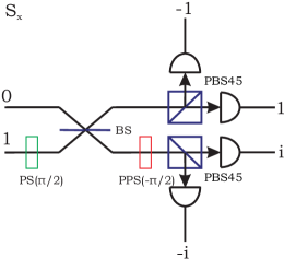
Figure 5.1: The setup which measures the operator $S_{x}$, for $d=4$. The $\pi/2$ phase shift (PS($\pi/2$)) in the path 1 ($|z+\rangle_{1}$) and the beam-splitter (BS) perform the path measurement, $\sigma_{x}^{(1)}$. The path state $|x+\rangle_{1}$ goes to the upper arm where the polarization is measured in the $\sigma_{x}^{(0)}$ basis with the polarizing beam-splitter which transmits $|x+\rangle_{0}$ (denoted as PBS45). In case of the path state $|x-\rangle_{1}$ the photon goes to the lower arm, where its $|z-\rangle_{0}$ polarization component is phase shifted by $-\pi/2$ (PPS($-\pi/2$)). Next, the photon enters PBS45, and is detected in one of its outputs. The eigenvalues corresponding to clicks of each detector are also written.

The eigenstates of the last five observables are maximally entangled states of the subsystems. Some of these observables, to keep the spectrum in the domain of fourth roots of unity, need to be multiplied by $\gamma\equiv\alpha_{4}^{1/2}=e^{i\pi/4}$. Take as an example the $S_{11}$ operator in the form $S_{11}=\gamma S_{x}S_{z}$. Its eigenstates are given by

$$\begin{array}[]{lcl}|0\rangle=\frac{1}{\sqrt{2}}\Big{(}|x+\rangle_{1}|z-\rangle_{0}-i\gamma|x-\rangle_{1}|z+\rangle_{0}\Big{)},&&|1\rangle=\frac{1}{\sqrt{2}}\Big{(}|x+\rangle_{1}|z+\rangle_{0}-i\gamma|x-\rangle_{1}|z-\rangle_{0}\Big{)},\\ |2\rangle=\frac{1}{\sqrt{2}}\Big{(}|x+\rangle_{1}|z-\rangle_{0}+i\gamma|x-\rangle_{1}|z+\rangle_{0}\Big{)},&&|3\rangle=\frac{1}{\sqrt{2}}\Big{(}|x+\rangle_{1}|z+\rangle_{0}+i\gamma|x-\rangle_{1}|z-\rangle_{0}\Big{)}.\end{array}$$ (5.48)

To distinguish between these states one needs to build an interferometer like the one in Fig. 5.2.

Figure 5.2: Mach-Zehnder interferometer, with a polarization rotator in one arm, followed by polarizing beam-splitters, is the most advanced device used in measurements of $S_{kl}$, for $d=4$. This setup, which measures the operator $\gamma S_{x}S_{z}$ (with $\gamma=e^{i\pi/4}$), distinguishes maximally entangled states of paths and polarizations. First, with the $\pi/2$ phase shift (PS($\pi/2$)) and the beam-splitter (BS), the $\sigma_{x}^{(1)}$ eigenstates are converted into $\sigma_{z}^{(1)}$ eigenstates. Next, the $\pi/4$ phase (PS($\pi/4$)) is applied in the lower arm, where $|x-\rangle_{1}$ is directed. In the upper arm polarization is rotated (with the plate $\curvearrowright$), such that in both arms it is the same. Finally, specific clicks behind the beam-splitter and polarizing beam-splitters distinguish the states (5.48).

The same setup measures $S_{22}$ and $S_{33}$, which commute with $S_{11}$. Finally, when different phase shifts are used, this setup also measures the remaining $S_{13}$ and $S_{31}$ observables.

To sum up, the most involved device, used in the measurements of generalized Pauli operators on a composite qudit encoded in two paths and polarization of a photon, involves a Mach-Zehnder interferometer with a polarization rotator in one arm, followed by polarizing beam-splitters (Fig. 5.2). Most of the observables are realizable with a single beam-splitter followed by polarizing beam-splitters.

Generally, it is possible to perform an arbitrary $S_{kl}$ measurement on polarized photons with many, $d_{1}$, accessible paths. With polarizing beam-splitters in each propagation path one transforms the initial polarization-path state $|j\rangle$ into a double-number-of-paths state $|p\rangle$, in $2d_{1}$ dimensional Hilbert space (each polarizing beam-splitter generates two distinct spatial modes). According to [112] one can always realize a unitary which brings the states $|p\rangle$ to the states of well-defined propagation direction. Thus, $2d_{1}$ detectors monitoring these final paths distinguish all the eigenvectors $|j\rangle$.

5.3 Appendix C: Spontaneous parametric down-conversion

In this section we describe how a polarization entangled state of two photons (which was used in the experimental falsification of the class of nonlocal theories) can be generated in a nonlinear crystal pumped with a laser field. The description is idealized, however it recovers all main features of the generated photons. This treatment was presented by the Sen family and Żukowski [113].

5.3.1 Crystal-field interaction

Consider an experiment in which a laser shines on a cubic crystal of volume $V=L^{3}$. Let us divide the volume into macroscopically small pieces $\delta V(\vec{x})$, which however include many atoms (or molecules) of the crystal. Since atoms are electrically neutral (so is the whole medium) the dominant part in the interaction Hamiltonian comes from the coupling between electric polarization of a local volume $\delta V(\vec{x})$, $\vec{P}(\vec{x},t)$, and a local electric field $\vec{E}(\vec{x},t)$:

$$H_{int}\sim\int_{V}d\vec{x}\textrm{ }\vec{P}(\vec{x},t)\cdot\vec{E}(\vec{x},t)=\int_{V}d\vec{x}\sum_{i=1}^{3}P_{i}(\vec{x},t)E_{i}(\vec{x},t).$$ (5.49)

In strong electromagnetic fields the polarization of certain crystals can depend on higher powers of the field:

$$P_{i}(\vec{x},t)=\sum_{j=1}^{3}\chi^{(1)}_{ij}E_{j}(\vec{x},t)+\sum_{j=1}^{3}\sum_{k=1}^{3}\chi^{(2)}_{ijk}E_{j}(\vec{x},t)E_{k}(\vec{x},t)+....$$ (5.50)

where one assumes the coefficients $\chi^{(m)}_{ijk...}$ are neither dependent on an actual position within the crystal nor on time, and that the polarization in point $\vec{x}$ depends on the field in the same point only. The two-photon generation process of interest is linked with the nonlinear term, $\chi^{(2)}_{ijk}$, in this expansion. Note that the electromagnetic field should not be too strong, as in that case even higher order emitions become non-negligible. The nonlinear interaction Hamiltonian can be found after inserting nonlinear dependence in (5.50) into (5.49), and reads:

$$H_{int}^{(2)}\sim\int_{V}d\vec{x}\sum_{i=1}^{3}\sum_{j=1}^{3}\sum_{k=1}^{3}\chi^{(2)}_{ijk}E_{i}(\vec{x},t)E_{j}(\vec{x},t)E_{k}(\vec{x},t).$$ (5.51)

The local field can be assumed to split into a classical and quantum part:

$$\vec{E}(\vec{x},t)=\vec{E}^{cl}(\vec{x},t)+\vec{E}^{qm}(\vec{x},t),$$ (5.52)

where the classical part describes the laser field, and the quantum part deals with a small number of photons. The laser light can be taken as a monochromatic plane wave linearly polarized along $\hat{x}$ direction:

$$\vec{E}^{cl}(\vec{x},t)=E_{x}\cos(\vec{k}_{0}\cdot\vec{x}-\omega_{0}t-\varphi)=E_{x}[e^{i(\vec{k}_{0}\cdot\vec{x}-\omega_{0}t-\varphi)}+c.c.],$$ (5.53)

where c.c. denotes the complex conjugate, $\vec{k}_{0}$ the wave vector and $\omega_{0}$ the angular frequency of the laser.

In general, one can write the quantum field in the interaction picture as:

$$\vec{E}^{qm}(\vec{x},t) = \sum_{p=1}^{2}\int d\vec{k}F(\omega)\hat{\epsilon}(\vec{k},p)a(\vec{k},p)e^{i(\vec{k}\cdot\vec{x}-\omega t)}+h.c.$$ (5.54)

$$\equiv \vec{E}^{(+)}(\vec{x},t)+\vec{E}^{(-)}(\vec{x},t),$$

where $F(\omega)=i/\sqrt{2\omega(2\pi)^{3}}$, the sum is taken over two orthogonal polarizations $\hat{\epsilon}(\vec{k},p)$, $\omega$ is the angular frequency of a photon the annihilation operator of which is denoted by $a(\vec{k},p)$, with $\vec{k}$ being the wave vector. The abbreviation $h.c.$ stands for Hermitian conjugate of a previous term, i.e. $\vec{E}^{(-)}(\vec{x},t)=[\vec{E}^{(+)}(\vec{x},t)]^{\dagger}$. The principal commutation rule for the creation and annihilation operators is given by:

$$\Big{[}a(\vec{k},p),a^{\dagger}(\vec{k}^{\prime},p^{\prime})\Big{]}=\delta_{p,p^{\prime}}\delta(\vec{k}-\vec{k}^{\prime}),\quad\Big{[}a^{\dagger}(\vec{k},p),a^{\dagger}(\vec{k}^{\prime},p^{\prime})\Big{]}=0,\quad\Big{[}a(\vec{k},p),a(\vec{k}^{\prime},p^{\prime})\Big{]}=0.$$

Since only two-photon emitions are of interest, after inserting the sum (5.52) of classical and quantum fields into the nonlinear Hamiltonian (5.51) and performing all the multiplications therein, one can focus on one of the terms with two creation operators [which come via the $\vec{E}^{(-)}(\vec{x},t)$ part of the quantum field]:

$$H_{SPDC}\sim\int_{V}d\vec{x}\sum_{i=1}^{3}\sum_{j=1}^{3}\sum_{k=1}^{3}\chi^{(2)}_{ijk}E_{i}^{cl}(\vec{x},t)E_{j}^{(-)}(\vec{x},t)E_{k}^{(-)}(\vec{x},t)+h.c..$$ (5.55)

Writting all the fields explicitly using formulas (5.53) and (5.54) one arrives at the interaction Hamiltonian describing the process of spontaneous parametric down-conversion. The terms involving two creation operators read:

$$H_{SPDC}\sim\sum_{j,k=1}^{3}\chi^{(2)}_{1jk}\sum_{p,p^{\prime}=1}^{2}\int d\vec{k}\int d\vec{k}^{\prime}\mathcal{G}(\vec{k},\vec{k}^{\prime},p,p^{\prime})a^{\dagger}(\vec{k},p)a^{\dagger}(\vec{k}^{\prime},p^{\prime})$$

$$\times\int_{V}d\vec{x}\Big{\{}e^{i\vec{x}\cdot(\vec{k}_{0}-\vec{k}-\vec{k}^{\prime})}e^{it(-\omega_{0}+\omega+\omega^{\prime})}e^{-i\varphi}+e^{i\vec{x}\cdot(-\vec{k}_{0}-\vec{k}-\vec{k}^{\prime})}e^{it(\omega_{0}+\omega+\omega^{\prime})}e^{i\varphi}\Big{\}},$$ (5.56)

with the coupling factor $\mathcal{G}(\vec{k},\vec{k}^{\prime},p,p^{\prime})=E_{x}\epsilon_{j}(\vec{k},p)\epsilon_{k}(\vec{k}^{\prime},p^{\prime})F(\omega)F(\omega^{\prime})$. The variables with index zero describe the pump field, those which are primed and unprimed describe two down-converted photons.

Let us perform the integration over the crystal volume in the Hamiltonian (5.56):

$$e^{it(-\omega_{0}+\omega+\omega^{\prime})}e^{-i\varphi}\int_{V}d\vec{x}e^{i\vec{x}\cdot(\vec{k}_{0}-\vec{k}-\vec{k}^{\prime})}+e^{it(\omega_{0}+\omega+\omega^{\prime})}e^{i\varphi}\int_{V}d\vec{x}e^{i\vec{x}\cdot(-\vec{k}_{0}-\vec{k}-\vec{k}^{\prime})}.$$ (5.57)

In the limit $V\to\infty$ the two integrands approach the Dirac delta $\delta(\pm\vec{k}_{0}-\vec{k}-\vec{k}^{\prime})$. For a finite size of the crystal one has approximate relation $\pm\vec{k}_{0}\approx\vec{k}+\vec{k}^{\prime}$. One can doubt about a physical meaning of the relation with the minus sign, in which case the generated photons propagate in the opposite direction to the pump field. Indeed this case is unphysical as it will be shown when considering the frequencies of the down-converted photons. Practical crystals are macroscopic, with $L$ of the order of a millimeter, and this relation (with a plus sign) holds perfectly. It is often quoted as the momentum conservation law.

Let us describe the time evolution generated by Hamiltonian (5.56). All states and operators are taken in the interaction (Dirac) picture, with the interaction Hamiltonian given by $H_{SPDC}$ (note that it explicitely depends on time, i.e. $H_{SPDC}=H_{SPDC}(t)$).

The generated two-photon state, $|\psi(t)\rangle_{12}$ (in the interaction picture), evolves according to the Schrödinger equation:

$$i\hbar\frac{d}{dt}|\psi(t)\rangle_{12}=H_{SPDC}(t)|\psi(t)\rangle_{12}.$$ (5.58)

Therefore:

$$|\psi(t_{f})\rangle_{12}-|\psi(t_{i})\rangle_{12}=\frac{1}{i\hbar}\int_{t_{i}}^{t_{f}}H_{SPDC}(t^{\prime})|\psi(t^{\prime})\rangle_{12}dt^{\prime},$$ (5.59)

where $t_{i}$ ($t_{f}$) denotes the initial (final) interaction time. The $H_{SPDC}$ Hamiltonian describes the interaction between the monochromatic plane wave and the quantum field initially in the vacuum state of no photons: $|\psi(t_{i})\rangle_{12}=|\Omega\rangle$. Since the monochromatic wave extends infinitely in time one puts for $t_{i}=-\infty$ and for $t_{f}=\infty$. In fact, the final time is a detection time, but since the two-photon state is always observed outside the crystal setting $t_{f}=\infty$ is a good approximation. Using the first order of the perturbation calculus one can replace $|\psi(t^{\prime})\rangle_{12}$ on the right-hand side with the initial vacuum state $|\Omega\rangle$. Thus the final two-photon state $|\Psi\rangle_{12}\equiv|\psi(t_{f}=\infty)\rangle_{12}$ reads:

$$|\Psi\rangle_{12}=|\Omega\rangle+\frac{1}{i\hbar}\int_{-\infty}^{\infty}H_{SPDC}(t^{\prime})dt^{\prime}|\Omega\rangle.$$ (5.60)

Inserting the Hamiltonian $H_{SPDC}$ and keeping in mind the momentum considerations one notes that the time-dependent part of the two-photon state is proportional to:

$$e^{-i\varphi}\delta(\vec{k}_{0}-\vec{k}-\vec{k}^{\prime})\int_{-\infty}^{\infty}dt^{\prime}e^{it^{\prime}(-\omega_{0}+\omega+\omega^{\prime})}+e^{i\varphi}\delta(-\vec{k}_{0}-\vec{k}-\vec{k}^{\prime})\int_{-\infty}^{\infty}dt^{\prime}e^{it(\omega_{0}+\omega+\omega^{\prime})}.$$ (5.61)

The two integrals are given by the Dirac delta $2\pi\delta(\pm\omega_{0}+\omega+\omega^{\prime})$. Thus the allowed frequencies of the emissions satisfy the relation $\pm\omega_{0}=\omega+\omega^{\prime}$. However, the case $-\omega_{0}=\omega+\omega^{\prime}$ requires at least one of the frequencies $\omega$ or $\omega^{\prime}$ to be negative. This is impossible to meet. The only physical situation left requires

$$\vec{k}_{0} \approx \vec{k}+\vec{k}^{\prime},$$ (5.62)

$$\omega_{0} = \omega+\omega^{\prime}.$$ (5.63)

The second equation expresses energy conservation law. These relations are known as phase matching conditions.

Additionally to phase matching conditions one has to take into account a dispersion relation for light moving in a medium. In general one has

$$\omega=|\vec{k}|c(\omega,p),$$ (5.64)

where $c(\omega,p)$ is the speed of light in a given medium. It is a function of polarization (birefringence effect) and angular frequency (normal and anomal dispersion). Together with the phase matching condition for frequencies this relation leads to

$$|\vec{k}_{0}|c(\omega_{0},p_{0})\approx|\vec{k}|c(\omega,p)+|\vec{k}^{\prime}|c(\omega^{\prime},p^{\prime}).$$ (5.65)

Only in specific directions one can expect correlated emissions. From now on we consider the energy degenerate case

$$\omega=\omega^{\prime}=\frac{\omega_{0}}{2},$$ (5.66)

in which both down-converted photons have the same frequency.

5.3.2 Path entanglement

Suppose that the polarizations of the emitted photons are the same (so called Type-I SPDC). Since we have also chosen their frequencies to be equal, both photons propagate with the same speed, $c(\omega,p)$, inside the crystal. In this case the dispiersion relation (5.65) reads:

$$|\vec{k}_{0}|c(\omega_{0},p_{0})\approx 2|\vec{k}|c(\omega,p).$$ (5.67)

In the medium in which $c(\omega_{0},p_{0})>c(\omega,p)$ one has $|\vec{k}_{0}|<2|\vec{k}|$. This, together with the wave vectors phase matching condition, implies that directions of emitted photons make the angle $\alpha=\frac{|\vec{k}|}{|\vec{k}_{0}|/2}=\frac{c(\omega_{0},p_{0})}{c(\omega,p)}$ with the direction of the pump beam. The photons are emitted on opposite sides of the cone centered on the beam (Fig. 5.3).

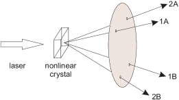
Figure 5.3: Type I SPDC. The two photons have the same polarization. They are emitted on the opposite sides of the cone centered on the laser beam. Since the actual propagation direction of a single photon is unknown the emerging state is entangled. With suitable pinholes outside the crystal one can generate the entangled state between arbitrary number of propagation directions. In this figure it is essentially $|1A\rangle|1B\rangle+|2A\rangle|2B\rangle$.

Their joint state outside the crystal can be found from the interaction Hamiltonian $H_{SPDC}$ to read:

$$|\Psi\rangle_{12}\sim\int d\vec{k}\mathcal{G}(\vec{k},\vec{k}_{0}-\vec{k},p,p)a^{\dagger}(\vec{k},p)a^{\dagger}(\vec{k}_{0}-\vec{k},p)|\Omega\rangle,$$ (5.68)

i.e. it is a coherent superposition of emitions into opposide directions of the cone, in which the actual direction of a single photon is not fixed. This is a “path” entangled state.

5.3.3 Polarisation entanglement

All the crystals in which parametric down-conversion takes place are birefringent. If the molecules of the medium are centro-symmetric the coefficients $\chi^{(2)}_{ijk}$ vanish, and one cannot observe the process.

For a suitable angle between the laser beam and the optical axis of the crystal the down-converted photons have orthogonal polarizations (Type II SPDC). One of them has polarization of the ordinary beam, the other - of the extraordinary beam. The photons with orthogonal polarizations appear on two different cones (Fig. 5.4).

Figure 5.4: Type II SPDC. The two photons have orthogonal polarizations. They are emitted on two different cones. Entangled state emerges from the intersection of the cones. Because of the birefringence of the crystal to see quantum interference one needs to compensate different time of flight of $H$ and $V$ polarized photons (not shown in this Figure).

Let us focus on the light generated in the intersection points of the cones. There, one of the photons has an orthogonal polarization to the other, but the polarization of a single photon is not defined. However, in principle one can learn the polarization of a single photon with the time-of-flight through the crystal measurement (since differently polarized photons propagate with different velocities in the birefringent media). Thus, to observe the polarization entanglement one has to erase the time-of-flight information. This can be achieved with a compensation outside the crystal. One simply rotates the polarization and lets the photons pass through a half-width crystal. The final state essentially reads [114]:

$$|\psi\rangle_{12}=\frac{1}{\sqrt{2}}\Big{[}|H\rangle_{1}|V\rangle_{2}+e^{i\phi}|V\rangle_{1}|H\rangle_{2}\Big{]},$$ (5.69)

where $H$ and $V$ denote horizontal and vertical polarization, respectively. The relative phase, $\phi$, can be arbitrarily engineered e.g. by using an additional phase shifter. This source was used to disprove the class of nonlocal theories of the main text.

Bibliography

- [1] A. Einstein, B. Podolsky, and N. Rosen, Phys. Rev. 47, 777 (1935).
- [2] J. S. Bell, Physics 1, 195 (1964).
- [3] J. F. Clauser, M. A. Horne, A. Shimony, and R. A. Holt, Phys. Rev. Lett. 23, 880 (1969).
- [4] J. F. Clauser and M. A. Horne, Phys. Rev. D 10, 526 (1974).
- [5] D. M. Greenberger, M. A. Horne, and A. Zeilinger, in Bell’s Theorem, Quantum Theory, and Conceptions of the Universe, edited by M. Kafatos, Kluwer Academic, Dordrecht, 69 (1989).
- [6] D. M. Greenberger, M. A. Horne, A. Shimony, and A. Zeilinger, Am. J. Phys. 58, 1131 (1990).
- [7] R. F. Werner and M. W. Wolf, Phys. Rev. A 64, 032112 (2001).
- [8] H. Weinfurter and M. Żukowski, Phys. Rev. A 64, 010102(R) (2001).
- [9] M. Żukowski and Č. Brukner, Phys. Rev. Lett. 88, 210401 (2002).
- [10] S. J. Freedman and J. F. Clauser, Phys. Rev. Lett. 28, 938 (1972).
- [11] A. Aspect, J. Dalibard, and G. Roger, Phys. Rev. Lett. 49, 1804 (1982).
- [12] G. Weihs, T. Jennewein, C. Simon, H. Weinfurter, and A. Zeilinger, Phys. Rev. Lett. 81, 5039 (1998).
- [13] M. A. Rowe, D. Kielpinski, V. Meyer, C. A. Sackett, W. M. Itano, C. Monroe, and D. J. Wineland, Nature 409, 791 (2001).
- [14] A. J. Leggett, Found. Phys. 33, 1469 (2003).
- [15] R. D. Gill, G. Weihs, A. Zeilinger, and M. Żukowski, Proc. Nat. Acad. Sci. USA, 9, 14632 (2002).
- [16] R. D. Gill, G. Weihs, A. Zeilinger, and M. Żukowski, Europhys. Lett. 61, 282 (2003).
- [17] C. H. Bennett, G. Brassard, C. Crépeau, R. Jozsa, A. Peres, and W. K. Wootters, Phys. Rev. Lett. 70, 1895 (1993).
- [18] C. H. Bennett and S. J. Wiesner, Phys. Rev. Lett. 69, 2881 (1992).
- [19] C.H. Bennet and G. Brassard, in Proceedings of the IEEE Int. Conf. on Computers, Systems and Signal Processing, Bangalore (1984).
- [20] A. K. Ekert, Phys. Rev. Lett. 67, 661 (1991).
- [21] C.H. Bennett, G. Brassard, and N. D. Mermin, Phys. Rev. Lett. 68, 557 (1992).
- [22] G. Brassard, Found. Phys. 33, 1593 (2003).
- [23] Č. Brukner, M. Żukowski, J.-W. Pan, and A. Zeilinger, Phys. Rev. Lett. 92, 127901 (2004).
- [24] N. J. Cerf, M. Bourennane, A. Karlsson, and N. Gisin, Phys. Rev. Lett. 88, 127902 (2002).
- [25] P. Trojek, C. Schmid, M. Bourennane, Č. Brukner, M. Żukowski, and H. Weinfurter, Phys. Rev. A 72, 50305(R) (2005).
- [26] A. Acin, N. Gisin, L. Masanes, and V. Scarani, Int. J. Quant. Inf. 2, 23 (2004).
- [27] J. F. Clauser and A. Shimony, Rep. Prog. Phys. 41, 1881 (1978).
- [28] N. D. Mermin, Phys. Rev. Lett. 65, 1838 (1990).
- [29] M. Ardehali, Phys. Rev. A 46, 5375 (1992).
- [30] A. V. Belinskii and D. N. Klyshko, Phys. Usp. 36, 653 (1993).
- [31] M. Żukowski, Č. Brukner, W. Laskowski, and M. Wieśniak, Phys. Rev. Lett. 88, 210402 (2002).
- [32] I. Pitowsky and K. Svozil, Phys. Rev. A 64, 014102 (2001).
- [33] C. Śliwa, Phys. Lett. A 317, 165 (2003).
- [34] D. Collins and N. Gisin, J. Phys. A: Math. Gen. 37, 1775 (2004).
- [35] M. Żukowski, Quant. Inf. Proc. 5, 287 (2006).
- [36] M. Żukowski, Phys. Lett. A 177 290 (1993).
- [37] N. Gisin, Phys. Lett. A 260 (1999);
- [38] S. Massar, Phys. Rev. A 65, 032121 (2002);
- [39] S. Massar, S. Pironio, J. Roland, and B. Gisin, Phys. Rev. A 66, 052112 (2002).
- [40] S. Massar and S. Pironio, Phys. Rev. A 68, 62109 (2003)
- [41] D. Bohm, Quantum Theory, Prentice-Hall, New York (1951).
- [42] T. K. Lo and A. Shimony, Phys. Rev. A 23, 3003 (1981).
- [43] J. S. Bell, Speakable and Unspeakable in Quantum Mechanics (Cambridge University Press) (1987).
- [44] A. Garg and N. D. Mermin, Phys. Rev. D 35, 3821 (1987).
- [45] J.-Å. Larsson, Phys. Rev. A 57, 3304 (1998).
- [46] J. Barrett, D. Collins, L. Hardy, A. Kent, and S. Popescu, Phys. Rev. A 66, 42111 (2002).
- [47] A. Kent, Phys. Rev. A 72, 12107 (2005).
- [48] P. G. Kwiat, P. H. Eberhard, A. M. Steinberg, and R. Y. Chiao, Phys. Rev. A 49, 3209 (1994).
- [49] S. F. Huelga, M. Ferrero, and E. Santos, Phys. Rev. A 51, 5008 (1995).
- [50] E. S. Fry, T. Walther, and S. Li, Phys. Rev. A 52, 4381 (1995).
- [51] J.-W. Pan, D. Bouwmeester, M. Daniell, H. Weinfurter, and A. Zeilinger, Nature 403, 515 (2000).
- [52] R. Horodecki, P. Horodecki, and M. Horodecki, Phys. Lett. A 200, 340 (1995).
- [53] A. Peres, Quantum Theory: Concepts and Methods, (Kluwer Academic Publishers, 1995).
- [54] N. Gisin, Phys. Lett. A 154, 201 (1991).
- [55] N. Gisin and A. Peres, Phys. Lett. A 162, 15 (1992).
- [56] Č. Brukner, M. Żukowski, and A. Zeilinger, quant-ph/0106119 (2001).
- [57] I. Pitowsky, Mathematical Programming 50, 395 (1991).
- [58] X.-H. Wu and H.-S. Zong, Phys. Lett. A 307, 262 (2003).
- [59] X.-H. Wu and H.-S. Zong, Phys. Rev. A 68, 32102 (2003).
- [60] A. Sen(De), U. Sen, M. Wieśniak, D. Kaszlikowski, and M. Żukowski, Phys. Rev. A 68, 62306 (2003).
- [61] M. Eibl, S. Gaertner, M. Bourennane, C. Kurtsiefer, M. Żukowski, and H. Weinfurter, Phys. Rev. Lett. 90, 200403 (2003).
- [62] D. Kaszlikowski, P. Gnaciński, M. Żukowski, W. Miklaszewski, and A. Zeilinger, Phys. Rev. Lett. 85, 4418 (2000).
- [63] W. Dür, Phys. Rev. Lett. 87, 230402 (2001).
- [64] M. Żukowski and D. Kaszlikowski, Phys. Rev. A 56, R1682 (1997).
- [65] D. Kaszlikowski, L. C. Kwek, J. Chen, and C. H. Oh, Phys. Rev. A 66, 52309 (2002).
- [66] A. Sen (De), U. Sen, and M. Żukowski, Phys. Rev. A 66, 62318 (2002).
- [67] K. Chen, S. Albeverio, and S.-M. Fei, Phys. Rev. A 74, 50101(R) (2006).
- [68] D. Bohm, Phys. Rev. 85, 166 (1952).
- [69] D. Bohm, Phys. Rev. 85, 180 (1952).
- [70] P. R. Holland, The Quantum Theory of Motion, (Cambridge University Press, Cambridge, U.K., 1993).
- [71] V. Scarani, and N. Gisin, Phys. Rev. Lett. 87, 117901 (2001).
- [72] M. Żukowski, Phys. Rev. A 62, 32101 (2000).
- [73] K. Mattle, H. Weinfurter, P. G. Kwiat, and A. Zeilinger, Phys. Rev. Lett. 76, 4656 (1996).
- [74] X. Fang, X. Zhu, M. Feng, X. Mao, and F. Du, Phys. Rev. A 61, 22307 (2000).
- [75] W. K. Wooters and W. H. Zurek, Nature 304, 188 (1982).
- [76] D. Bouwmeester, J.-W. Pan, K. Mattle, M. Eibl, H. Weinfurter, and A. Zeilinger, Nature 390, 575 (1997).
- [77] D. Boschi, S. Branca, F. De Martini, L. Hardy, and S. Popescu, Phys. Rev. Lett. 80, 1121 (1998).
- [78] Y.-H. Kim, S. P. Kulik, and Y. Shih, Phys. Rev. Lett. 86, 1370 (2001).
- [79] M. D. Barrett, J. Chiaverini, T. Schaetz, J. Britton, W. M. Itano, J. D. Jost, E. Knill, C. Langer, D. Leibfried, R. Ozeri, and D. J. Wineland, Nature 429, 737 (2004).
- [80] P. W. Shor, in Proceedings of the 35th Annual Symposium on the Foundations of Computer Science, p. 124.
- [81] G. Vernam, J. Amer. Inst. Elec. Eng. 55, 109 (1926).
- [82] C. E. Shannon, Bell Syst. Tech. J. 28, 656 (1949).
- [83] N. Gisin, G. Ribordy, W. Tittel, and H. Zbinden, Rev. Mod. Phys. 74, 145 (2002).
- [84] C. H. Bennett, F. Bessette, G. Brassard, L. Salvail, and J. Smolin, J. Crypto. 5, 3 (1992).
- [85] P. A. Hiskett, D. Rosenberg, C. G. Peterson, R. J. Hughes, S. Nam, A. E. Lita, A. J. Miller, and J. E. Nordholt, New J. Phys. 8, 193 (2006).
- [86] A. Poppe, A. Fedrizzi, R. Ursin, H. R. Böhm, T. Lörunser, O. Maurhardt, M. Peev, M. Suda, C. Kurtsiefer, H. Weinfurter, T. Jennewein, and A. Zeilinger, Opt. Express 12, 3865 (2004).
- [87] I. Csiszár, and J. Körner, IEEE Trans. Inf. Theory IT-24, 339 (1978).
- [88] C.-S. Niu and R. B. Griffiths, Phys. Rev. A 60, 2764 (1999).
- [89] V. Scarani and N. Gisin, quant-ph/0104016 (2001).
- [90] W.-Y. Hwang, Phys. Rev. A 71, 052329 (2005).
- [91] H. Bechmann-Pasquinucci and A. Peres, Phys. Rev. Lett. 85, 3313 (2000);
- [92] D. Bruß and C. Macchiavello, Phys. Rev. Lett. 88, 127901 (2002).
- [93] W. K. Wooters and B. D. Fields, Ann. Phys. (N. Y.) 191, 363 (1989).
- [94] S. Bandyopadhyah, P. O. Boykin, V. Roychowdhury, and F. Vatan, Algorithmica 34, 512 (2002).
- [95] A. C.-C. Yao, in Proceedings of the 11th Annual ACM Symposium on Theory of Computing, 209 (1979).
- [96] R. Cleve and H. Buhrman, Phys. Rev. A 56, 1201 (1997).
- [97] H. Buhrman, W. van Dam, P. Høyer, and A. Tapp, Phys. Rev. A 60, 2737 (1999).
- [98] H. Buhrman, R. Cleve, and W. van Dam, SIAM J. Comput. 30, 1829 (2001).
- [99] L. Hardy and W. van Dam, Phys. Rev. A 59, 2635 (1999).
- [100] Č. Brukner, M. Żukowski, and A. Zeilinger, Phys. Rev. Lett. 89, 197901 (2002).
- [101] E. Kushilevitz and N. Nisan, Communication Complexity, Cambridge University Press, New York, 1997.
- [102] E. F. Galvão, Phys. Rev. A. 65, 012318 (2001).
- [103] D. Collins, N. Gisin, N. Linden, S. Massar, and S. Popescu, Phys. Rev. Lett. 88, 040404 (2002).
- [104] M. Żukowski, A. Zeilinger, and M. A. Horne, Phys. Rev. A 55, 2564 (1997).
- [105] A. Acin, T. Durt, N. Gisin, and J. I. Latorre, Phys. Rev. A 65, 052325 (2002).
- [106] A. Peres, Found. Phys. 29, 589 (1999).
- [107] J. P. Jarrett, Noûs 18, 569 (1984).
- [108] A. Zeilinger, H. J. Bernstein, D. M. Greenberger, M. A. Horne, and M. Żukowski in Quantum Control and Measurement, edited by H. Ezawa and Y. Murayama (Elsevier, Amsterdam, 1993).
- [109] A. Zeilinger, M. Żukowski, M. A. Horne, H. J. Bernstein, and D. M. Greenberger in Quantum Interferometry, edited by F. DeMartini and A. Zeilinger (World Scientific, Singapore, 1994).
- [110] D. I. Fivel, Phys. Rev. Lett. 74, 835 (1995).
- [111] A. O. Pittenger and M. H. Rubin, Phys. Rev. A 62, 32313 (2000).
- [112] M. Reck, A. Zeilinger, H. J. Bernstein, and P. Bertani, Phys. Rev. Lett. 73, 58 (1994).
- [113] A. Sen(De), U. Sen, and M. Żukowski, Phys. Rev. A 68, 62301 (2003).
- [114] P. G. Kwiat, K. Mattle, H. Weinfurter, A. Zeilinger, A. V. Sergienko, and Y. Shih, Phys. Rev. Lett. 75, 4337 (1995).