Perturbation Expansion for Option Pricing with Stochastic Volatility

Abstract

We fit the volatility fluctuations of the S&P 500 index well by a Chi distribution, and the distribution of log-returns by a corresponding superposition of Gaussian distributions. The Fourier transform of this is, remarkably, of the Tsallis type. An option pricing formula is derived from the same superposition of Black-Scholes expressions. An explicit analytic formula is deduced from a perturbation expansion around a Black-Scholes formula with the mean volatility. The expansion has two parts. The first takes into account the non-Gaussian character of the stock-fluctuations and is organized by powers of the excess kurtosis, the second is contract based, and is organized by the moments of moneyness of the option. With this expansion we show that for the Dow Jones Euro Stoxx $50$ option data, a $\Delta$-hedging strategy is close to being optimal.

I Introduction

The purpose of this paper is to develop analytic expressions for option-pricing of markets with fluctuating volatilities of a given distribution. There are several good reasons for considering the statistical properties of volatilities. For instance, a number of important models of price changes include explicitly their time-dependence, for example the Heston model Heston1 , or the famous ARCH Engle82 , GARCH Bollerslev86 , and multiscale GARCH Z-L03 models. Changes in the daily volatility are qualitatively well explained by models relating volatility to the amount of information arriving in the market at a given time Jacquier . There is also considerable practical interest in volatility distributions since they provide traders with an essential quantitative information on the riskiness of an asset B-P ; Bouchaud94 . As such it provides a key input in portfolio construction.

Unlike returns which are correlated only on very short time scales Fama70 of a few minutes and can roughly be approximated by Markovian process, the volatility changes exhibit memory with time correlations up to many years Ding93 ; Dacorogna93 ; Liu97 ; TIMX . In Ref. Liu97 it was shown that the Standard & Poor 500 (hereafter S&P 500) volatility data can be fitted quite well by a log-normal distribution. This result appears to be at odds with the fact that the log-normal shape of the distribution typically signalizes a multiplicative nature Bunde96 of an underlying stochastic process. This is rather surprising in view of efficient market theories Fama70 which assume that the price changes are caused by incoming new information about an asset. Such information-induced price changes are additive and should not give rise to multiplicative process. We cure this contradiction by observing that the same volatility data can be fitted equally well by a Chi distribution feller ; wik . In Appendix A we show that corresponding sample paths follow the additive rather than multiplicative Itō stochastic process. With the help of Itō’s lemma one may show (cf. Appendix A) that the variance $v(t)=\sigma^{2}(t)$ follows the Itō’s stochastic equation

$$\textrm{d}v(t)\ =\ \gamma(t)[\nu(t)-\mu(t)v(t)-a(v(t),\mu(t),\nu(t))]\textrm{d}t\ +\ \sqrt{2\gamma(t)v(t)}\;\!\textrm{d}W(t)\,.$$ (1)

where $W(t)$ is a Wiener process. Here $\gamma(t),\mu(t)$ and $\nu(t)$ are arbitrary non-singular positive real functions on $\mathbb{{R}}^{+}$. Function $a(\ldots)$ is non-singular in all its arguments and it tends to zero at large $t$’s. From the corresponding Fokker-Planck equation one may determine the time-dependent distribution of $v$ which reads

$$f_{\mu(t),\nu(t)}(v)~{}=~{}\frac{1}{\Gamma(\nu(t))}~{}[\mu(t)]^{\nu(t)}v^{\nu(t)-1}e^{-\mu(t)v}\,,\;\;\;\;\;\;\mbox{with}\;\;\;\;\;\int_{0}^{\infty}\textrm{d}v\ f_{\mu,\nu}(v)~{}=~{}1.$$ (2)

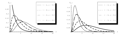
Figure 6: Gamma distribution for various values of $\mu$ and $\nu$, with average $\bar{v}=\nu/\mu=\beta$,  variance $\overline{(v-\bar{v})^{2}}=\nu/\mu^{2}$, skewness $\overline{(v-\bar{v})^{3}}=2/\sqrt{\nu}$, and excess kurtosis $\overline{(v-\bar{v})^{4}}/\overline{(v-\bar{v})^{2}}^{2}-3=6/\nu$.

The distribution $f_{\mu,\nu}(v)$ is the normalized Gamma probability density feller , whose profile is shown in Fig. 6. It has an average $\bar{v}=\nu/\mu$,  a variance $\overline{(v-\bar{v})^{2}}=\nu/\mu^{2}$, a skewness $\overline{(v-\bar{v})^{3}}=2/\sqrt{\nu}$, and an excess kurtosis $\overline{(v-\bar{v})^{4}}/\overline{(v-\bar{v})^{2}}^{2}-3=6/\nu$ (see, e.g., Refs.feller ; HK ). The Gamma distribution (2) will play a key role in the following reasonings. The Chi distribution $\rho(\sigma,t)$ is related with the Gamma distribution through the relation

$$\rho(\sigma,t)\ =\ 2\sigma f_{\mu(t),\nu(t)}(\sigma^{2})\,.$$ (3)

Often is the functional form (3) itself called a Gamma distribution. To avoid potential ambiguities, we shall confine in the following to the name Chi distribution. The derivation of $\rho(\sigma,t)$ from the underlying additive process, rather than a multiplicative process, shows that the Chi distribution is well compatible with efficient markets.

The Gamma distributions for fluctuations of $v$ allow us to generate an entirely new class of option pricing formulas. For this we use the well-known fact of non-equilibrium statistical physics kubo , that the density matrix of a system with fluctuating temperature can be written as a density matrix for the system with fixed temperature averaged with respect to a temperature distribution function. Path integrals conveniently facilitate this task HK . With the help of the so-called Schwinger trick we show that if the distribution of the inverse-temperatures of the log-returns is of the Gamma type, the distribution in momentum space is of the Tsallis type. To put this observation into a relevant context, we recall that Tsallis distributions in momentum space enjoy a key role in statistical physics as being optimal in an information theoretical sense: given prior information only on the covariance matrix and a so-called escort parameter, they contain the least possible assumptions, i.e., they are the most likely unbiased representation of the provided data. Some background material on this subject is reviewed in Appendix C. The observed connection with Tsallis distribution in momentum space can be fruitfully used to address the issue of the time-compounded density function for stock fluctuations with Chi distributed volatility. The Markovian property of the market prices then simply translates to product of distributions in momentum space. At the level of the distributions of log-returns, this automatically gives rise to the correct Chapman-Kolmogorov equation for Markovian processes. The time-compounded distribution function constructed by convolution of integrals represents the desired measure of stock fluctuations at given time $t$.

It should be emphasized that since the distribution of log-returns is related to the Tsallis distribution in momentum space by a Fourier transform, the log-return data do not inherit the heavy tails of the Tsallis distribution in momentum space. In this respect our approach is quite different from data analysis based on a Tsallis distribution of log-returns, such as the so-called ‘non-extensive thermostatic” Borland . The formal advantage of our model lies in its optimal use of the mathematical machinery of the Black-Scholes theory. In particular, one still has the option pricing formula that is linear in the spot probability of the strike-price payment. Put and call options still obey the put-call parity relation, and the $\Delta$-hedge still coincides with the spot probability that multiplies the asset price in the Black-Scholes formula. On the other hand, the desired features such as peaked middles of financial asset fluctuations and semi-fat tails are present for sufficiently long times. The latter ensures that ensuing option prices can differ noticeably from the Black-Scholes curves for rather long expiration dates (days or even moths) despite the validity of central limit theorem (CLT). One may thus expect our formulation to be useful, e.g., for short or mid-term maturity options (“mesoscopic” time lags).

The paper is organized as follows. In Section II we fit the high-frequency data set of the volatility fluctuations in the S&P 500 index from 1985 to 2007 to a Chi distribution. We also show that this fit holds well for different time averaging windows. In Section III we represent the distribution of log-returns as a superposition of Gaussian distributions with the above volatility behavior and find that the associated distribution in momentum space is of the Tsallis type. By assuming further that the compounded stock fluctuations over longer times are Markovian we obtain in Section IV the corresponding natural martingale measure. With it we derive an option-pricing formula as a superposition of Black-Scholes expressions. The departure from Black-Scholes results is expressed as a sum of two qualitatively different expansions: expansion in powers of the excess curtosis and expansion in momenta of moneyness. The former represents the expansion in market characteristics while the latter is an expansion based on contract characteristics. In Section V we determine the crossover time below which our option prices differs from Black-Scholes. Comparisons with observed log-returns are presented in Section VI. There we show that for the Dow Jones Euro Stoxx 50 data the amount of the residual risk in the $\Delta$-hedge portfolio is very small and that the crossover time is roughly $7-8$ months. Section VII, finally, is devoted to conclusions. For reader’s convenience we also include three appendices. In Appendix A we solve and discuss the Fokker-Planck equations that are associated with stochastic equations for the volatility and variance presented in Introduction. In Appendix B we deal with some mathematical manipulations needed in Section IV. In Appendix C we present some basics for Rényi and THC statistics to better understand some remarks in the main body of the paper.

II Empirical motivation

Our work is motivated by data sets on volatility distributions extracted from the S&P 500 stock market index. We briefly remind the reader the procedure for obtaining these numbers. A detailed description can be found in Ref.Liu97 and citations therein.

It is well known that the autocorrelation function of stock market returns decays exponentially with a short characteristic time – typically few trading minutes (e.g., $\approx 4$ min. for S&P 500 index). Hence the log-returns $R$ are basically uncorrelated random variables, nevertheless, they are not independent since higher-order correlations reveal a richer structure. In fact, empirical analysis of financial data confirms Liu97 that the autocorrelation function of non-linear functions of $R$, such as $|R|$ or $R^{2}$, has much longer decorrelation time (memory) spanning up to several years (few months for S&P 500 index). These observations imply that a realistic model for the return-generating processes should account for a non-linear dependence in the returns. The latter can be most naturally achieved via some additional memory-bearing stochastic process. Most simply, this subsidiary process involves directly the volatility.

One may bypass a construction of the volatility model by trying to define a “judicious” volatility estimator directly from financial time series. Difficulty resides, however, in the fact that although the volatility is supposed to be a measure of the magnitude of market fluctuations, it is not immediately clear how such a measure should be quantified. Among many definitions present in the literature pasquini98 we focuss here on the estimator proposed in Ref.Liu97 . There one defines the volatility $\sigma_{T}(t_{\eta})$, at a given time $t_{\eta}$ as the arithmetic average of the absolute value of the log-returns

$$R(t_{n})\ \equiv\ \ln\frac{S(t_{n}+\Delta t)}{S(t_{n})}\ \cong\ \frac{S(t_{n}+\Delta t)-S(t_{n})}{S(t_{n})}\,,$$ (4)

over some time window of the length $T\equiv n\Delta t$ ($n\in\mathbb{N}^{+}$, $\Delta t$ is the sampling interval), i.e.,

$$\sigma_{T}(t_{\eta})\ \equiv\ \frac{1}{n}\sum_{m=\eta}^{n-1+\eta}|R(t_{m})|\,,\;\;\;\;\;(t_{\eta}=\eta\Delta t,\;t_{m}=m\Delta t)\,.$$ (5)

Because (5) is basically a forward-time mean value of absolute returns, it may indeed serve as a good measure of market fluctuations.

With this $\sigma_{T}(t)$ we can construct the corresponding volatility probability density function according to a relative frequency prescription:

$$\rho_{T}(\sigma)\Delta\sigma\ =\ \frac{\mbox{\# $\sigma_{T}(t)\in[\sigma,\sigma+\Delta\sigma]$}}{n}\,.$$ (6)

In the limit of the very large time window $T$, one might expect $\rho_{T}(\sigma)$ to approach a Gaussian distribution, since the CLT holds also for correlated time series Beran94 , although with an often slower convergence than for independent processes Potters96 .

There is, however, a logical caveat in the definition (5). The observed volatility fluctuations have a spuriously superposed pattern caused by intra-day fluctuations. This is because over the day, the market activity is large at the beginning and at the end, but exhibits a broad minimum around a noon admati88 . Since the volatility is supposed to measure the magnitude of the market activity, this intra-day pattern should be removed in order to avoid false correlations. This can be remedied by considering the normalized returns Liu97

$$R_{\rm{nor}}(t_{n})\equiv\frac{\ln[S(t_{n}+\Delta t)/S(t_{n})]}{\langle|\ln[S(t_{n}+\Delta t)/S(t_{n})]|\rangle}\cong\frac{S(t_{n}+\Delta t)-S(t_{n})}{S(t_{n})}\bigg{/}\!\left\langle\left|\frac{S(t_{n}+\Delta t)-S(t_{n})}{S(t_{n})}\right|\right\rangle\!.$$ (7)

Here $\langle\ldots\rangle$ is the average over the whole sequence of trading days, i.e.,

$$\langle|\ln[S(t_{n}+\Delta t)/S(t_{n})]|\rangle\ \equiv\ \frac{1}{N_{\rm{td}}}\sum_{j=1}^{N_{\rm{td}}}|\ln[S_{j}(t_{n}+\Delta t)/S_{j}(t_{n})]|\,,$$ (8)

with $S_{j}(t_{n})$ denoting the spot price of the index at the time $t_{n}$ on the $j$th trading day, and $N_{\rm{td}}$ denotes the total number of trading days. So in (7) each spot return is divided by its natural “spot return scale”. The corresponding normalized volatility is then defined as

$$\sigma_{T\rm{nor}}(t_{\eta})\ \equiv\ \frac{1}{n}\sum_{m=\eta}^{n-1+\eta}|R_{\rm{nor}}(t_{m})|\,.$$ (9)

This is the quantity whose distribution will be discussed here (we omit the subscript “nor” in the following). To this end we shall examine the data set for the S&P 500 stock market index. Data in question were gathered over the period of 22 years from Jan 1985 to Jan 2007 at roughly $5$ minute increments. The corresponding empirical time sequence is seen in Fig. 1.

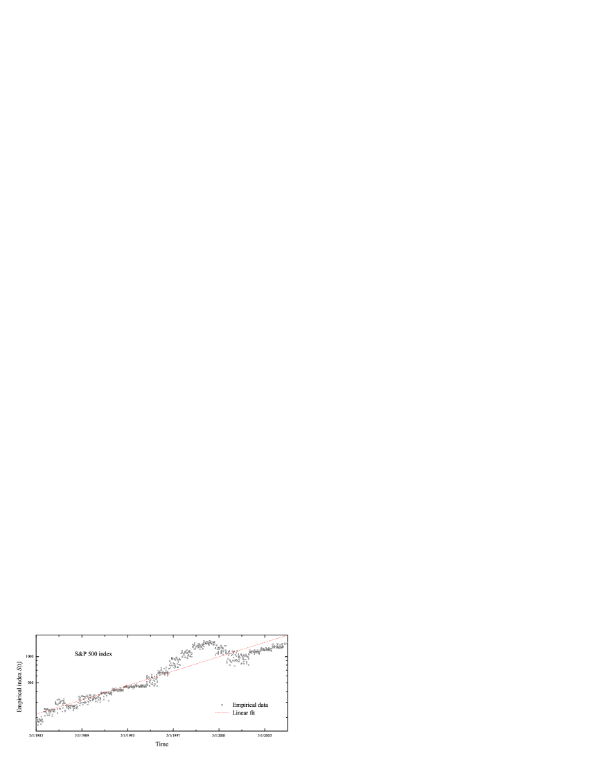
Figure 1: Logarithmic plot of the S&P 500 index $S(t)$ over $22$ years (5 January 1985 - 5 January 2007) with sampling intervals $\Delta t=5$ min. The linear fit shows the typical exponential growth at an annual rate of $\approx 15\%$. Only end-of-day prices are shown.

 

With the help of the prescription (5) we obtain the volatility for the above S&P 500 index data shown in Fig. 2.

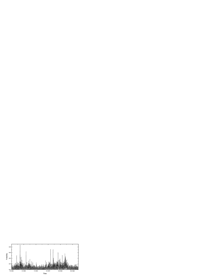
Figure 2: Volatility $\sigma_{T}(t)$ of S&P 500 index over $22$ years (5 January 1985 - 5 January 2007) with sampling intervals $\Delta t=5~{}$min. and time window $T=300~{}$min., i.e., roughly one trading day. Only $3000$ volatility values are plotted.

 

The corresponding normalized volatility $\sigma_{T\rm{nor}}(t)$ is shown in Fig. 3. The normalization was taken with respect to $N_{\rm{td}}=5550$ (i.e., approximate number of trading days between 5 Jan. 1985 - 5 Jan. 2007).

Figure 3: Normalized volatility $\sigma_{T\rm{nor}}(t)$ of S&P 500 index over $22$ years (5 January 1985 - 5 January 2007) with sampling interval $\Delta t=5~{}$min., $N_{\rm{td}}=5550$, and time window $T=300~{}$min., i.e., roughly one trading day. Only $1000$ volatility values are plotted.

 

Figure 4 shows the volatility probability density function $\rho_{T}(\sigma)$ with the time window $T=300~{}$min. While it is seen that $\rho_{T}(\sigma)$ can be well fitted with the Log-normal function (as proposed in Ref.Liu97 ), the Chi distribution gives a better fit in the central part and is of roughly the same quality in the tail part. Because the value of the volatility quantifies the asset risk, Fig. 4 implies that the Log-normal fit slightly overestimates, while the Chi distribution slightly underestimates the large risks. In addition, the functions $\mu$ and $\nu$ that parameterize the Chi (and Gamma) distribution (cf. Eq.(3)) are in the observed time windows proportional to $T$, i.e. $\mu(T)=\mu T$ and $\nu(T)=\nu T$. This tendency is confirmed in Fig. 5 which shows the corresponding variance distribution $\rho_{T}(v)$ for

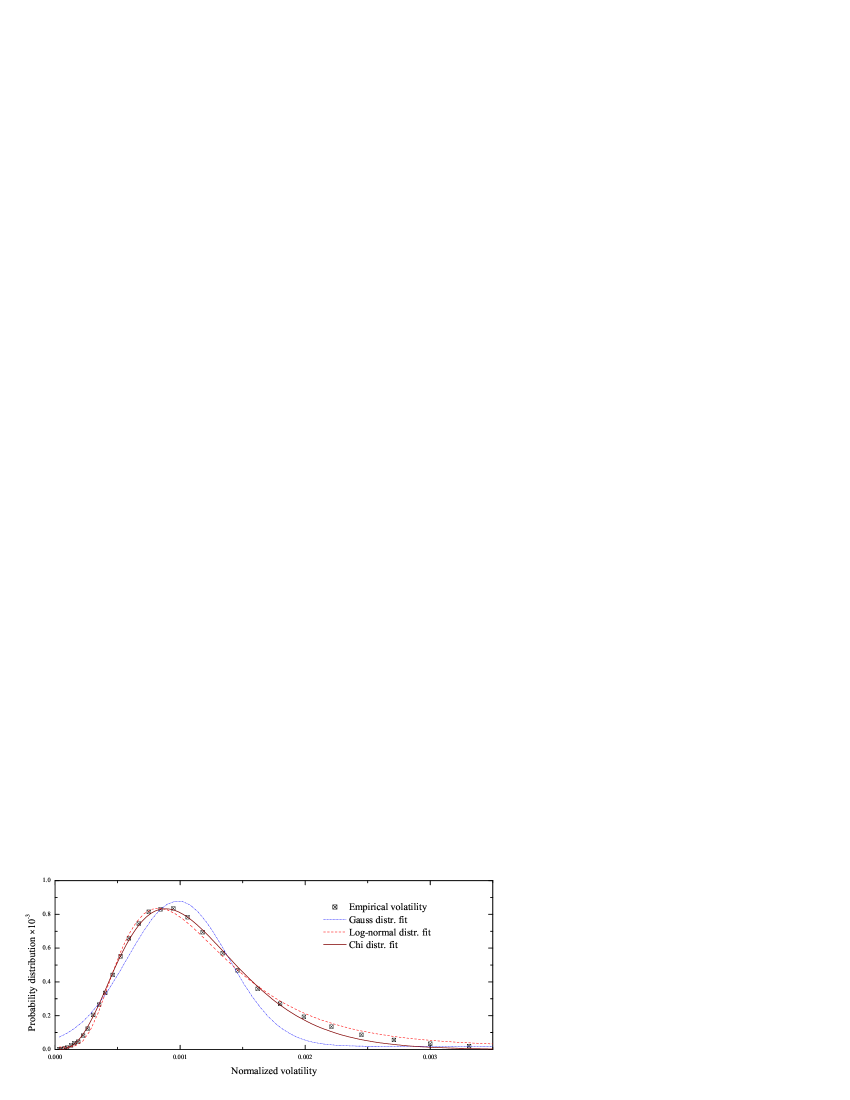
Figure 4: Best Gaussian, Log-normal and Chi-distribution fit for the S&P 500 empirical volatility. The time window $T=300~{}$min.

 

three different window sizes $T$. For better comparison we use the scaled distribution form, $\Gamma(T\nu)\rho_{T}(v)/(T\mu)$ as a function of $T\mu v+(1-T\nu)\ln(T\mu v)$, with $\mu=E(v)/Var(v)$ and $\nu=E^{2}(v)/Var(v)$ ($E$ and $Var$ are empirical mean and variance, respectively). After the above scaling, empirical variance distributions, with $T=300,600$ and $900~{}$min. nicely “collapse” to the canonical exponential $\exp(-x)$ (i.e., Gamma distribution with both mean and variance equal to $1$), confirming thus the assumed Gamma distribution behavior for rather long averaging times.

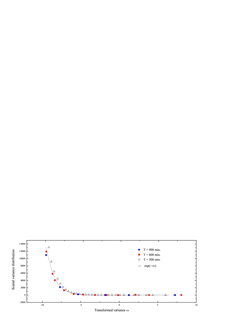
Figure 5: The scaled variance distribution for different window sizes $T$. The scaled distribution is plotted as a function of the transformed volatility $v_{tr}=T\mu v+(1-T\nu)\ln(T\mu v)$.

 

In the limit of very long $T$, one expects that $\rho_{T}(\sigma)$ becomes Gaussian, due to CLT. For the times considered here, however, the Chi distribution fits the data better than a Gaussian one. We see thus that the long-range correlations in the volatility fluctuations considerably slow down the convergence towards the Gaussian distribution. The conclusions that one my draw from this is that, even for large times, the tail of $\rho_{T}(\sigma)$ has a fairly large amount of distribution (or information) that cannot be ignored. This will provide a key input in generalizing the Black–Scholes pricing formula in Section IV.

III Theoretical digression – Tsallis’ density operator

We have mentioned before the result in statistical physics kubo that a density matrix of a system with fluctuating temperature can be written as a density matrix with fixed temperature averaged with respect to some temperature distribution function. This technique was recenly proposed as a natural frame for composing non-Gaussian price distributions REMPI0 and for deriving option pricing formulas REPI .

Consider the Gaussian distribution of the Brownian motion of a particle of unit mass as a function of the inverse temperature $\beta_{G}\equiv 1/T$:

$$\rho_{\rm G}(x_{b},x_{a};\beta_{G})=\frac{1}{\sqrt{2\pi\beta_{G}}}\ e^{-(x_{b}-x_{a})^{2}/2\beta_{G}}\,.$$ (10)

We use natural units in which the Boltzmann constant $k_{B}$ has the value 1. The variance $v\equiv\sigma^{2}$ of this distribution is obviously equal to $\beta_{G}$. Following Ref. REMPI0 we form a superposition of these distributions as an integral over different inverse temperatures, i.e., different variances $v$:

$$\rho_{\delta}(x_{b},x_{a};\beta)~{} = \ \int_{0}^{\infty}\textrm{d}v~{}f_{\mu,1/\delta}(v)\frac{1}{\sqrt{2\pi v}}\ e^{-(x_{b}-x_{a})^{2}/2v},~{}~{}~{}\;\;\;\;\beta\ \equiv\ \bar{v}\ =\ \nu/\mu\,,$$ (11)

where $f_{\mu,\nu}(v)$ is the Gamma distribution defined in (2) whose average lies at $\bar{v}=\nu/\mu$. The subscript $\delta$ of the distribution characterizes the ratio

$$\delta=\frac{1}{\nu}=\frac{\overline{(v-\bar{v})^{2}}}{\bar{v}^{2}},$$ (12)

a quantity which we shall call the spread of the Gamma distribution. In terms of the integration variable $s=\mu v$, we can rewrite (11) in the form

$$\rho_{\delta}(x_{b},x_{a};\beta)\ =\ \frac{1}{\Gamma(1/\delta)}\int_{0}^{\infty}\frac{\textrm{d}s}{s}~{}s^{1/\delta}e^{-s}\sqrt{\frac{\mu}{2\pi s}}\ e^{-(x_{b}-x_{a})^{2}\mu/2s}\,.$$ (13)

In quantum mechanics, one writes such a distribution in a notation due to Dirac as a matrix element

$$\rho(x_{b},x_{a};\beta)\ \equiv\ \langle x_{b}|\hat{\rho}(\beta)|x_{a}\rangle\,,$$ (14)

of a density operator

$$\hat{\rho}(\beta)~{}\equiv~{}\frac{1}{\Gamma(1/\delta)}\int_{0}^{\infty}\frac{\textrm{d}s}{s}~{}s^{1/\delta}e^{-s}e^{-\delta\beta\,s\hat{H}}\,,~{}~{}~{}~{}~{}\beta\equiv\nu/\mu=1/\mu\delta\,,$$ (15)

where

$$\hat{H}\ \equiv\ \frac{\hat{p}^{2}}{2}\ =\ -\frac{\partial_{x}^{2}}{2}\,,$$ (16)

is the Hamilton operator of a free particle of unit mass. The integral over $s$ can be done (as in the so-called Schwinger trick HK ) and yields:

$$\hat{\rho}(\beta)~{}=~{}\left[1\ +\ \beta\delta\hat{H}\right]^{-1/\delta}\,.$$ (17)

This is the (un-normalized) Tsallis density operator (cf. Appendix B) with a so-called escort parameter $q$ related to the spread parameter $\delta$ by $q\equiv 1+\delta$, and an inverse Tsallis temperature $\beta$ equal to $\nu/\mu$.

 

In the limit $\delta\rightarrow 0$ where $q\rightarrow 1_{+}$, the Tsallis operator (17) converges to an exponential

$$\hat{\rho}(\beta)\ \rightarrow\ e^{-\beta_{G}\hat{H}},\;\;\;\;\;\;\;\;\beta_{G}\ =\ \beta|_{q=1}\,,$$ (18)

and the distribution function (13) becomes Gaussian. The corresponding limit of the Gamma distribution (2) is a $\delta$-function:

$$f_{\mu,\nu}(x)\approx\sqrt{\frac{\mu}{2\pi x}}\!\left(\frac{\mu x}{\nu}\right)^{\nu-1/2}e^{-\nu(\mu x/\nu-1)}\approx\frac{1}{\sqrt{2}~{}x}~{}\delta\!\left(\sqrt{\frac{\mu x}{\nu}-1-\log\frac{\mu x}{\nu}}\right)=\delta\!\left(x-\frac{\nu}{\mu}\right)\!.$$ (19)

Hence the density matrix (11) approaches for $\delta\rightarrow 0$ the canonical density matrix of the Gibbs-Boltzmann statistics of the inverse temperature $\nu/\mu=\beta_{G}$. Note, that in order to ensure that $\beta_{G}$ is finite in the small-$\delta$ limit, $\mu$ must behave as $1/\delta\beta_{G}$ at $\delta\rightarrow 0$. The reader may easily check that a superposition of the type (11) exists also for distributions of Bashkirov’s 1-st version of thermostatics (cf. Appendix B). In that case $0<q<1$, $\delta=1-q$ and $\beta\mapsto\tilde{\beta}$. In the limit $q\rightarrow 1_{-}$ the density matrix becomes again a Gibbs-Boltzmann canonical density matrix.

IV Generalized option pricing formula

Consider a continuously tradable stock and assume that the stock fluctuations over short time intervals $\Delta t_{0}$ such as $\Delta t_{0}=1$ day are described by the stationary Tsallis density operator (17). The time $\Delta t_{0}$ will from now on play the role of a time unit. We now analyze the modifications of the Black-Scholes formula for pricing European call options CallE brought about by the fluctuations of the volatilities. After a time $t>0$ (always in units of $\Delta t_{0}$) the stock fluctuations follow a Tsallis density operator

$$[\hat{\rho}(\beta)]^{t}~{} = ~{}Z^{-t}\left[1~{}+~{}\beta\delta\hat{H}\right]^{-t/\delta}~{}=\ \frac{Z^{-t}}{\Gamma\left(t/\delta\right)}\int_{0}^{\infty}\frac{\textrm{d}s}{s}~{}s^{t/\delta}e^{-s[1+\beta\delta\hat{H}]}$$ (20)

$$= ~{}\left(\frac{t}{\beta\delta}\right)^{\!t/\delta}\frac{Z^{-t}}{\Gamma\left(t/\delta\right)}\int_{0}^{\infty}\frac{\textrm{d}v}{v}~{}v^{t/\delta}e^{-tv\mu}e^{-tv\hat{H}}\,,$$

where $Z$ is a normalization factor. In the sequel we shall allow for a drift of the returns by extending the Hamiltonian operator (16) to

$$H=p^{2}/2+pr_{x_{W}}/v\,,$$ (21)

where $r_{W}$ is the growth rate of the riskfree investment, and $r_{x_{W}}=r_{W}+v/2$ is the associated growth rate of its logarithm. The parameter $\beta$ equals to $1/\delta\mu$, as before. The matrix elements of (20) yield the time-compounded probability density

$$P_{\delta}(x_{b},t_{b};x_{a},t_{a})~{}=~{}\langle x_{b}|[\hat{\rho}(\beta)]^{t}|x_{a}\rangle\,,\;\;\;~{}~{}~{}~{}t\equiv t_{b}-t_{a}>0\,.$$ (22)

Being the matrix element of the product of operators $\hat{\rho}(\beta)$. $P_{\delta}(x_{b},t_{b};x_{a},t_{a})$ fulfills trivially the Chapman-Kolmogorov relation for a Markovian process

$$P_{\delta}(x_{b},t_{b};x_{a},t_{a})\ =\ \int_{-\infty}^{\infty}\textrm{d}x\ P_{\delta}(x_{b},t_{b};x,t_{c})P_{\delta}(x,t_{c};x_{a},t_{a})\,,\;\;\;\;\;t_{b}>t_{c}>t_{a}\,.$$ (23)

For Gaussian stock fluctuations with the Hamiltonian (21), the riskfree martingale measure density has the form HK

$$P^{(M,r_{W})}_{v}(x_{b},t_{b};x_{a},t_{a})=\Theta(t_{b}-t_{a})\frac{e^{-r_{W}(t_{b}-t_{a})}}{\sqrt{2\pi v(t_{b}-t_{a})}}\ \exp\left\{-\frac{[x_{b}-x_{a}-r_{x_{W}}(t_{b}-t_{a})]^{2}}{2v(t_{b}-t_{a})}\right\}$$

$$\mbox{\hskip 56.9055pt}=\Theta(t_{b}-t_{a})e^{-r_{W}(t_{b}-t_{a})}\int_{x(t_{a})=x_{a}}^{x(t_{b})=x_{b}}{\mathcal{D}}x~{}\exp\left\{-\frac{1}{2v}\int_{t_{a}}^{t_{b}}[\dot{x}-r_{x_{W}}]^{2}\textrm{d}t\right\}.$$ (24)

The corresponding time-compounded version of the superposition (11) can be directly written as

$$P_{\delta}(x_{b},t_{b};x_{a},t_{a})~{}=~{}\int_{0}^{\infty}\!\!\textrm{d}v~{}f_{t\mu,\ \!t/\delta}(v)\!~{}P_{v}^{(M,r_{W})}(x_{b},t_{b};x_{a},t_{a})\,.$$ (25)

Correctness of the latter can be verified by combining (20), (22), and (24). The result is REMPI0

$$P_{\delta}(x_{b},t_{b};x_{a},t_{a})~{}=~{}\int_{0}^{\infty}\!\!\textrm{d}v~{}f_{t\mu,\ \!t/\delta}(v)\!~{}P_{v}^{(M,r_{W})}(x_{b},t_{b};x_{a},t_{a})$$

$$\mbox{\hskip 14.22636pt}=~{}\frac{e^{-(r_{W}t+\Delta x)/2}(2\mu)^{t/\delta}}{\sqrt{\pi}\,\Gamma\left(t/\delta\right)}\!\left(\frac{\sqrt{1+8\,\mu}}{|\Delta x-r_{W}t|}\right)^{\!\!1/2-t/\delta}\!\!K_{1/2-t/\delta}\!\!~{}\left(|\Delta x-r_{W}t|~{}\frac{\sqrt{1+8\,\mu}}{2}\right)\!,$$ (26)

with $\Delta x\equiv x_{b}-x_{a}$ and $t_{b}>t_{a}$. The measure density (26) has for $|\Delta x|\gg 1$ the asymptotic behavior of the Erlang distribution feller :

$$P_{\delta}(x_{b},t_{b};x_{a},t_{a})~{}\approx~{}\exp\left(-\frac{|\Delta x|}{2}\sqrt{1+8\,\mu}-\frac{\Delta x}{2}\right)~{}|\Delta x|^{-1+(t_{b}-t_{a})/\delta}\,,$$ (27)

which has a semi-fat tail (see Fig. 7). It should be noted that the exponential suppression ensures that all momenta are finite. This fact is an important ingredient in showing that (26) represents indeed the riskfree martingale measure density. The actual proof of the latter can be found in Ref. HK .

Figure 7: Normalized measure density (26); for various values of $\mu$ and $\delta$ at fixed expiration time and $\langle\sigma^{2}\rangle$ (left), for different expiration times at fixed $\delta$ and $\mu$ (right). We set the riskless interest rate $r_{W}$ to be $12\%$.

 

From the martingale measure (26), we now calculate the option price at an arbitrary earlier time $t_{a}$ via the evolution equation

$$O_{\delta}(x_{a},t_{a})~{}=~{}\int_{-\infty}^{\infty}\textrm{d}x_{b}~{}O(x_{b},t_{b})P_{\delta}(x_{b},t_{b};x_{a},t_{a})\,.$$ (28)

The value of the option at its expiration date $t_{b}$ is given by the difference between the underlying stock price $S_{b}\equiv S(t_{b})$ on expiration date and the strike price $E$, i.e.,

$$O(x_{b},t_{b})~{}=~{}\Theta(S_{b}-E)(S_{b}-E)~{}=~{}\Theta(x_{b}-x_{E})\left(e^{x_{b}}-e^{x_{E}}\right)\,,$$ (29)

where $x_{E}\equiv\log E$. Heaviside function $\Theta(x)$ ensures that the owner of the option will exercise his right to buy the stock only if he profits, i.e., only when $S_{b}-E$ is positive.

For Gaussian fluctuations of variance $v$, formula (28) is evaluated with the measure (24) and yields directly the Black-Scholes option pricing formula B-P :

$$O_{v}^{(BS)}(x_{a},t_{a})~{}=~{}S(t_{a})\Phi(y^{+}_{v})~{}-~{}e^{-r_{W}(t_{b}-t_{a})}E\Phi(y^{-}_{v})\,,$$ (30)

where $\Phi(y)$ represents the cumulative normal distribution and

$$y^{\pm}_{v}~{}=~{}\frac{\log[S(t_{a})/E]~{}+~{}\left(r_{W}\pm\mbox{$\frac{1}{2}$}v\right)(t_{b}-t_{a})}{\sqrt{v(t_{b}-t_{a})}}\,.$$ (31)

The generalization to the present semi-heavy tail distribution is obtained from the superposition REMPI0

$$O_{\delta}(x_{a},t_{a})~{}=~{}\int_{0}^{\infty}\!\!\textrm{d}v~{}f_{t\mu,\ \!t/\delta}(v)~{}O^{(BS)}_{v}(x_{a},t_{a})\,,\;\;\;\;\;\;\;\;\;\;\;t>0\,.$$ (32)

At this stage one should realize that integration in (32) acts only on the $\Phi(y^{\pm}_{v})$ parts of $O^{(BS)}_{v}(x_{a},t_{a})$. This allows to write the option price in the Black-Scholes-like form, namely

$$O_{\delta}(x_{a},t_{a})~{}=~{}S(t_{a})\Phi^{(+)}_{v}~{}-~{}e^{-r_{W}(t_{b}-t_{a})}E\Phi^{(-)}_{v}\,,$$ (33)

where $\Phi^{(+)}_{v}$ and $\Phi^{(-)}_{v}$ are Gamma-smeared versions of the functions $\Phi(y^{+}_{v})$ and $\Phi(y_{v}^{-})$, respectively. For $\delta\rightarrow 0$, the new functions reduce, of course, to the un-smeared ones due to the limit (19).

Let us now do the smearing operation for $\Phi^{(+)}_{v}$:

$$\Phi^{(+)}_{v}~{} = ~{}\int_{0}^{\infty}\textrm{d}v~{}f_{t\mu,t/\delta}(v)\Phi(y_{v}^{+})\ =~{}\int_{0}^{\infty}\textrm{d}v~{}f_{t\mu,t/\delta}(v)\int_{-\infty}^{y_{v}^{+}}\frac{\textrm{d}\xi}{\sqrt{2\pi}}\ e^{-\xi^{2}/2}$$ (34)

$$= ~{}\int_{0}^{\infty}\textrm{d}v~{}f_{t\mu,t/\delta}(v)\int_{-\infty}^{\infty}\frac{\textrm{d}\xi}{\sqrt{2\pi}}~{}\Theta(y_{v}^{+}-\xi)~{}e^{-\xi^{2}/2}.$$

By expressing the Heaviside function as

$$\Theta(x)=\int_{-\infty}^{\infty}\frac{\textrm{d}p}{2\pi i}\ \frac{1}{p-i0_{+}}\ e^{ipx},$$ (35)

and using Sokhotsky’s formula

$$\frac{1}{p-i0_{+}}~{}=~{}{\cal{P}}\!\left(\frac{1}{p}\right)~{}+\ i\pi\delta(p)\,,$$ (36)

where ${\cal P}$ denotes the principal value of the integral, we perform the integral over $\xi$ and obtain SEE

$$\Phi^{(+)}_{v}~{} = ~{}\frac{1}{2}~{}+~{}{{\cal P}}\int_{-\infty}^{\infty}\frac{\textrm{d}p}{2\pi i}~{}F^{(+)}_{t\mu,t/\delta}(p,A)~{}\frac{e^{-p^{2}/2}}{p}\,.$$ (37)

Here $F^{(+)}_{t\mu,t/\delta}(p,A)$ is the integral

$$F^{(+)}_{t\mu,t/\delta}(p,A)\ \equiv\ \int_{0}^{\infty}\textrm{d}v~{}f_{t\mu,t/\delta}(v)\ e^{ipy_{v}^{+}}\,.$$ (38)

This is evaluated as follows. We perform a change of variables from $v$ to $\omega\equiv\sqrt{vt}$, and define $A\equiv\log[S(t_{a})/E]+r_{W}t$, then we have

$$F^{(+)}_{t\mu,t/\delta}(p,A) = 2\frac{\mu^{t/\delta}}{\Gamma(t/\delta)}\int_{0}^{\infty}\textrm{d}\omega\ \omega^{2t/\delta-1}~{}e^{-\mu\omega^{2}}\ \exp\left[i\frac{p}{2}\left(\omega+\frac{2A}{\omega}\right)\right]$$ (39)

$$\equiv ~{}2\frac{\mu^{t/\delta}}{\Gamma(t/\delta)}~{}g^{(+)}_{\mu}(p,A)~{}.$$

In order to calculate $g^{(+)}_{\mu}(p,A)$ we observe that the following integral can immediately be done:

$$\int_{0}^{\infty}\textrm{d}\mu~{}\mu^{s-1}g^{(+)}_{\mu}(p,A)~{}=~{}\Gamma(s)\int_{0}^{\infty}\textrm{d}\omega~{}\omega^{2t/\delta-2s-1}\ \exp\left[i\frac{p}{2}\left(\omega+\frac{2A}{\omega}\right)\right]\,.$$ (40)

Let us first assume that $p>0$ and Arg$(A)=0$ and perform the substitution $\omega=\sqrt{2A}~{}\!\exp u$. This yields directly

$$\int_{0}^{\infty}\textrm{d}\mu~{}\mu^{s-1}g^{(+)}_{\mu}(p,A)~{} = \ \Gamma(s)(2A)^{t/\delta-s}\int_{-\infty}^{\infty}\textrm{d}u\ e^{ip\sqrt{2A}\cosh u-(2s-2t/\delta)u}$$ (41)

$$= ~{}i\pi\Gamma(s)(e^{-i\pi}2A)^{t/\delta-s}H^{(1)}_{2s-2t/\delta}(p\sqrt{2A})\,,\;\;\;\;\;\;\;\;\;\;\;\;\;\;(p>0)\,,$$

where $H^{(1)}_{\alpha}(z)$ is the Hankel function of the first kind Watson . This result holds for $\Re(s)>t/\delta-1/2$. Similarly we obtain for $p<0$:

$$\int_{0}^{\infty}\textrm{d}\mu~{}\mu^{s-1}g^{(+)}_{\mu}(p,A)~{} = ~{}-i\pi\Gamma(s)(e^{i\pi}2A)^{t/\delta-s}H^{(2)}_{2s-2t/\delta}(-p\sqrt{2A})\,,\;\;\;\;\;\;\;\;\;\;\;\;\;\;(p<0)\,,$$ (42)

where $H^{(2)}_{\alpha}(z)$ is the Hankel function of the second kind Watson . The result is valid for $\Re(s)<t/\delta+1/2$.

Knowing these integrals, we find the function $g^{(+)}_{\mu}(p,A)$ itself with the help of the Mellin inverse transform:

$$g^{(+)}_{\mu}(p,A)=\int_{c-i\infty}^{c+i\infty}\frac{\textrm{d}s}{2\pi i}\ \mu^{-s}\!\left\{\begin{array}[]{l}~{}~{}\,i\pi\Gamma(s)(e^{-i\pi}2A)^{t/\delta-s}H^{(1)}_{2s-2t/\delta}(p\sqrt{2A}),~{}~{}~{}~{}p>0,\\[5.69054pt] -i\pi\Gamma(s)(e^{i\pi}2A)^{t/\delta-s}H^{(2)}_{2s-2t/\delta}(-p\sqrt{2A}),~{}~{}~{}~{}p<0.\end{array}\right\}$$ (45)

where $c\in(t/\delta-1/2,t/\delta+1/2)$. Inserting this back into (39) and (37) one can write for $\Phi^{(+)}_{v}$:

$$\!\!\!\!\!\!\!\!\!\!\!\!\!\!\!\!\!\!\!\!\!\!\!\!\!\!\!\!\!\!\!\!\!\!\!\!\!\!\!\!\!\!\!\!\!\!\!\!\!\!\!\!\!\!\!\Phi^{(+)}_{v} = \frac{1}{2}+\frac{\mu^{t/\delta}}{\Gamma(t/\delta)}\ \!{{\cal P}}\!\!\int_{-\infty}^{\infty}\frac{\textrm{d}p}{2\pi i}\frac{e^{-p^{2}/2}}{p}\int_{c-i\infty}^{c+i\infty}\!\!\textrm{d}s\ \Gamma(s)\mu^{-s}\!\left\{\begin{array}[]{l}(e^{-i\pi}2A)^{t/\delta-s}H^{(1)}_{2s-2t/\delta}(p\sqrt{2A})\!\!\!\!\!\!\!\!\!\!\!\!\!\!\\[5.69054pt] -(e^{i\pi}2A)^{t/\delta-s}H^{(2)}_{2s-2t/\delta}(-p\sqrt{2A})\end{array}\right\}\!\!\!\!\!\!\!$$ (49)

$$= \frac{1}{2}+\frac{\mu^{t/\delta}}{\Gamma(t/\delta)}\int_{c-i\infty}^{c+i\infty}\!\!\textrm{d}s~{}\Gamma(s)\mu^{-s}(2A)^{t/\delta-s}\int_{0_{+}}^{\infty}\frac{\textrm{d}p}{2\pi i}\frac{e^{-p^{2}/2}}{p}\!\!\!\!\!\!\!\!\!\!\!\!\!\!\!\!\!\!\!\!\!\!\!\!\!\!\!$$

$$\mbox{\hskip 56.9055pt}\times\left[e^{i\pi(s-t/\delta)}H_{2s-2t/\delta}^{(1)}(p\sqrt{2A})+e^{i\pi(t/\delta-s)}H_{2s-2t/\delta}^{(2)}(p\sqrt{2A})\right].\!\!\!\!\!\!\!\!\!\!\!\!\!\!\!\!\!\!\!\!\!\!\!\!\!\!\!\!\!\!\!\!\!\!\!\!\!\!\!\!\!\!\!\!\!\!\!\!\!\!\!$$

Decomposing the Hankel functions into Bessel functions of first kind,

$$H_{\nu}^{(1,2)}(z)\ \equiv\ \pm\frac{J_{-\nu}(z)\ -\ e^{\mp i\pi\nu}J_{\nu}(z)}{i\sin(\nu\pi)}\,,$$ (50)

this becomes

$$\!\!\!\!\!\!\!\!\!\!\!\!\!\!\!\!\!\!\!\!\!\!\Phi^{(+)}_{v} = \frac{1}{2}+\frac{(2A\mu)^{t/\delta}}{\Gamma(t/\delta)}~{}\!\int_{c-i\infty}^{c+i\infty}\!\!~{}\frac{\textrm{d}s}{2\pi i}~{}\frac{\ \Gamma(s)(2A\mu)^{-s}}{\cos[\pi(t/\delta-s)]}~{}\!\int_{0_{+}}^{\infty}\textrm{d}p~{}\frac{e^{-p^{2}/2}}{p}~{}$$ (51)

$$\mbox{\hskip 113.81102pt}\times\left[J_{2s-2t/\delta}(p\sqrt{2A})+J_{2t/\delta-2s}(p\sqrt{2A})\right].\!\!\!\!\!\!\!\!\!\!$$

The $p$-integral can now be easily performed yielding

$$\frac{1}{\cos(\pi\zeta)}\int_{0_{+}}^{\infty}\textrm{d}p\ \frac{e^{-p^{2}/2}}{p}\left\{\begin{array}[]{l}J_{2\zeta}(p\sqrt{2A})\\ J_{-2\zeta}(p\sqrt{2A})\end{array}\right\}$$ (54)

$$\mbox{\hskip 17.07182pt}=~{}\frac{1}{2\sqrt{\pi}\zeta}\left\{\begin{array}[]{ll}\!\left(\frac{A}{4}\right)^{\zeta}\Gamma\!\left(\mbox{ $\!\!\frac{1}{2}$}-\zeta\right)\!\!~{}_{1\!}F_{1}(\zeta,1+2\zeta,-A),&\hbox{~{}~{}~{}$\Re~{}\zeta>0$}\\[5.69054pt] \!-\left(\frac{A}{4}\right)^{-\zeta}\Gamma\!\left(\mbox{ $\!\!\frac{1}{2}$}+\zeta\right)\!\!~{}_{1\!}F_{1}(-\zeta,1-2\zeta,-A),&\hbox{~{}~{}~{}$\Re~{}\zeta<0$}\end{array}\right\},$$ (57)

where $\zeta\equiv s-t/\delta$. The function $\!\!\!~{}_{1\!}F_{1}(a,b,z)$ is the Kummer confluent hypergeometric function Buchholtz . Note also that the fundamental strip $c\in(t/\delta-1/2,t/\delta+1/2)$ is for $\zeta$ in the upper expression reduced to $c\in(0,t/\delta+1/2)$, while for the lower expression $c\in(t/\delta-1/2,0)$.

We now perform $s$-integral in (51), and obtain

$$\!\!\!\!\!\!\Phi^{(+)}_{v}~{}=~{}\frac{1}{2}~{}+~{}h^{(+)}_{1}(\mu,t/\delta,A)~{}-~{}h^{(+)}_{2}(\mu,t/\delta,A)\,,$$ (58)

with

$$\mbox{}h^{(+)}_{1}(\mu,t/\delta,A)~{}=~{}\frac{1}{2\Gamma(t/\delta)\sqrt{\pi}}~{}\sum_{\mathrm{Res}}\frac{\Gamma(\zeta+t/\delta)}{\zeta}\left(8\mu\right)^{-\zeta}\Gamma\!\left(\mbox{ $\!\!\frac{1}{2}$}-\zeta\right)\!~{}_{1\!}F_{1}(\zeta,1+2\zeta,-A)\,,$$

$$\mbox{}h^{(+)}_{2}(\mu,t/\delta,A)~{}=~{}\frac{1}{2\Gamma(t/\delta)\sqrt{\pi}}~{}\sum_{\mathrm{Res}}\frac{\Gamma(\zeta+t/\delta)}{{\zeta}}\left(\frac{A^{2}\mu}{2}\right)^{-\zeta}\!\!\Gamma\!\left(\zeta+\mbox{ $\!\!\frac{1}{2}$}\right)\!~{}_{1\!}F_{1}(-\zeta,1-2\zeta,-A).$$ (59)

To compute the residues of the poles of $h^{(+)}_{1}$ and $h^{(+)}_{2}$ we need to decide in what way the poles are enclosed in the complex plane. Taking into account Stirling’s large-argument limit of the Gamma functions:

$$\frac{\Gamma(\zeta+t/\delta)\Gamma(\mbox{ $\!\!\frac{1}{2}$}-\zeta)}{\zeta}~{}\approx~{}\zeta^{t/\delta-3/2},\;\;\;\;\;\mbox{}\;\;\;\frac{\Gamma(\zeta+t/\delta)\Gamma(\mbox{ $\!\!\frac{1}{2}$}+\zeta)}{\zeta}~{}\approx~{}\left(\frac{\zeta}{e}\right)^{2\zeta}\zeta^{t/\delta-3/2}\,,$$ (60)

for $|\zeta|\rightarrow\infty$ ($|\mbox{Arg}(\zeta)|<\pi$), and the fact that the asymptotic behavior of $~{}_{1\!}F_{1}$ for large $|\zeta|$ is given by Kummer’s second formula [see, e.g., Ref. Luke Eq. (4.8.16)]

$$~{}_{1\!}F_{1}(\pm\zeta,1\pm 2\zeta,-A)~{}\approx~{}e^{-A/2},\;\;\;\;\;|\mbox{Arg}(\zeta)|~{}<~{}\pi\,,$$

$$~{}_{1\!}F_{1}(\zeta,1+2\zeta,-A)\;\;\;\;\;\ \mbox{for}\;\;\;\;\;\;\zeta~{}=~{}-1,-2,-3,-4,\ \ldots\;\;\;\;\mbox{undefined}\,,$$ (61)

we obtain that the contour closure of $h^{(+)}_{2}$ depends entirely on the behavior of the Gamma functions. In fact, due to previous asymptotics we must close the contour in $h^{(+)}_{2}$ to the left as the value of the contour integral around the large arc is zero in the limit of infinite radius. Due to $(8\mu)^{-\zeta}$ term $h^{(+)}_{1}$ closes the contour to the right. There are only simple poles contributing to $h^{(+)}_{1}$, which lie at $\zeta=(2n+1)/2,\;n\in{\mathbb{N}}\equiv(0,1,2,\dots)$. If we assume for a moment that $t/\delta\not=1/2+l,\;l\in{\mathbb{N}}$, then the only singularities of $h^{(+)}_{2}$ are due to simple poles at $\zeta=-1/2-m,\;m\in{\mathbb{N}}$ and $\zeta=-t/\delta-k,\;k\in{\mathbb{N}}$. Consequently we can write

$$\Phi^{(+)}_{v} = \frac{1}{2}\left[1~{}+~{}\sqrt{\frac{\bar{v}\delta}{2\pi}}\sum_{n=0}^{\infty}\frac{(t/\delta)_{n+1/2}(1/2)_{n}}{(1)_{2n+1}}\left(-\frac{\bar{v}\delta}{2}\right)^{\!\!n}\!~{}_{1\!}F_{1}\left(n+\frac{1}{2},2n+2,-A\right)\right.$$ (62)

$$\mbox{}+\left.~{}A\sqrt{\frac{2}{\pi\bar{v}\delta}}\sum_{n=0}^{\infty}\frac{(t/\delta)_{-n-1/2}(1/2)_{n}}{(1)_{2n+1}}\left(-\frac{2A^{2}}{\bar{v}\delta}\right)^{\!\!n}\!~{}_{1\!}F_{1}\left(n+\frac{1}{2},2n+2,-A\right)\right.$$

$$\mbox{}+\left.\frac{1}{\cos(\pi t/\delta)}\left(\frac{2A^{2}}{\delta\bar{v}}\right)^{\!\!t/\delta}\sum_{n=0}^{\infty}\frac{(t/\delta)_{n}}{(1)_{2n+2t/\delta}(1)_{n}}\left(\frac{2A^{2}}{\delta\bar{v}}\right)^{\!\!n}\!~{}_{1\!}F_{1}\left(n+\frac{t}{\delta},2n+1+2\frac{t}{\delta},-A\right)\right]\!,$$

where we have set $\bar{v}\equiv\langle v\rangle=\langle\sigma^{2}\rangle$ and used the Pochhammer symbols $(z)_{k}~{}\equiv~{}{\Gamma(k+z)}/{\Gamma(z)}\,$. If $\delta$ is very small, or $t$ very large, we can use the asymptotic behavior $(t/\delta)_{z}\rightarrow(t/\delta)^{z}$ and the fact that the sum in the third line of (62) tends to zero due to strong suppression by $1/(1)_{2n+t/\delta}$. In this case (62) reduces to

$$\Phi^{(+)}_{v}~{}=~{}\frac{1}{2}\left[1~{}+~{}\sqrt{\frac{2}{\pi}}\ y_{\bar{v}}^{+}\!~{}_{1\!}F_{1}\left(\frac{1}{2},\frac{3}{2},-\frac{(y_{\bar{v}}^{+})^{2}}{2}\right)\right]~{}=~{}\Phi(y_{\bar{v}}^{+})\,,~{}~{}~{}~{}\bar{v}=\beta\,.$$ (63)

The calculation of $\Phi^{(-)}_{v}$ is similar and is relegated to Appendix A. Here we state only the result:

$$\Phi^{(-)}_{v}~{} = ~{}\frac{1}{2}\left[1~{}-~{}\sqrt{\frac{\delta\bar{v}}{2\pi}}\sum_{n=0}^{\infty}\frac{(t/\delta)_{n+1/2}(1/2)_{n}}{(1)_{2n+1}}\left(-\frac{\bar{v}\delta}{2}\right)^{\!\!n}\!~{}_{1\!}F_{1}\left(n+\frac{1}{2},2n+2,A\right)\right.$$ (64)

$$\mbox{}+\left.~{}A\sqrt{\frac{2}{\pi\delta\bar{v}}}\sum_{n=0}^{\infty}\frac{(t/\delta)_{-n-1/2}(1/2)_{n}}{(1)_{2n+1}}\left(-\frac{2A^{2}}{\bar{v}\delta}\right)^{\!\!n}\!~{}_{1\!}F_{1}\left(n+\frac{1}{2},2n+2,A\right)\right.$$

$$\mbox{}+\left.\frac{1}{\cos(\pi t/\delta)}\left(\frac{2A^{2}}{\delta\bar{v}}\right)^{\!\!t/\delta}\sum_{n=0}^{\infty}\frac{(t/\delta)_{n}}{(1)_{2n+2t/\delta}(1)_{n}}\left(\frac{2A^{2}}{\bar{v}\delta}\right)^{\!\!n}\!~{}_{1\!}F_{1}\left(n+\frac{t}{\delta},2n+1+2\frac{t}{\delta},A\right)\right]\!.$$

In Appendix A we also show that for small $\delta$, or large $t$, $\Phi^{(-)}_{v}$ approaches the cumulative normal distribution $\Phi(y_{\bar{v}}^{-})$. The asymptotic behaviors ensure us that the $\delta\rightarrow 0_{+}$ limit leads back to the original Black-Scholes formula, as it should.

Another interesting situation arises for small $A$, where $S(t_{a})\approx Ee^{-r_{W}(t_{b}-t_{a})}$. Using the fact that $\!~{}_{1\!}F_{1}(a,b,0)=1$, and that we may neglect for small $A$ the last two sums in Eq.(62) and Eq.(64), we obtain that both $\Phi^{(+)}_{v}$ and $\Phi^{(-)}_{v}$ approach the cumulative normal distributions $\Phi(y_{\bar{v}}^{+}\rangle)|_{A=0}$ and $\Phi(y_{\bar{v}}^{-})|_{A=0}$, respectively, implying that $O_{\delta}(x_{a},t_{a})\rightarrow O^{(BS)}(x_{a},t_{a})|_{A=0}$. Options with $A=0$ are known as at-the-money-forward options, i.e. options whose strike price is equal to the current, prevailing price in the underlying forward market. Inasmuch, whenever the option is at-the-money-forward we regain back the formula of Black and Scholes. Since many real transactions in the over-the-counter markets are quoted and executed at or near at-the-money-forward McMillan02 , this explains some of the empirical support for the Black-Scholes model .

In this connection it is interesting to note that for put options, where the terminal condition is

$$O(x_{b},t_{b})~{}=~{}\Theta(E-S(t_{b}))(E-S(t_{b}))\,,$$ (65)

we would have obtained the pricing equation in the form

$$O_{\delta}(x_{a},t_{a})~{}=~{}Ee^{-r_{W}(t_{b}-t_{a})}(1-\Phi^{(-)}_{v})-S(t_{a})(1-\Phi^{(+)}_{v})\,.$$ (66)

This shows that our option-pricing model fulfills important consistency condition known as the put-call parity relation B-P

$$O^{P}_{\delta}\!(x_{a},t_{a})~{}=~{}O^{C}_{\delta}\!(x_{a},t_{a})-S(t_{a})+Ee^{-r_{W}(t_{b}-t_{a})}\,,$$ (67)

where $O^{P}_{\delta}$ and $O^{C}_{\delta}$ denote put and call options, respectively. Consequently, the case when $A\approx 0$ can be equally phased as a situation with $O^{C}_{\delta}(x_{a},t_{a})\approx O^{P}_{\delta}(x_{a},t_{a})$. We shall further see in the following section that the expansion factor $A/\sqrt{\bar{v}\delta}$ is directly related to the so-called moneyness of the options.

Moneyness is a measure of the degree to which an option is likely to have a nonzero value at the expiration date. In the Black-Scholes formula, the moneyness (measured in the units of standard deviation) is defined by B-P

$$m_{\rm BS}~{}=~{}\frac{y_{v}^{+}~{}+~{}y_{v}^{-}}{2}~{}=~{}\frac{\log[S(t_{a})/E]~{}+~{}r_{W}t}{\sigma\sqrt{t}}~{}=~{}\frac{A}{\sqrt{vt}}\,.$$ (68)

For at-the-money-forward options, the moneyness is zero. A positive value of $m_{\rm BS}$ corresponds to in-the-money-forward options (i.e., options with positive monetary value) while a negative value represents out-of-the-money options.

In our case $v=\sigma^{2}$ is a random variable and for given $t$ it is distributed according to the Gamma distribution $f_{t\mu,t/\delta}(v)$. We may easily calculate the momenta of $|m_{\rm BS}|$. The odd moments are

$$\frac{\langle|m_{\rm BS}|^{2n+1}\rangle}{(2n+1)!}~{}=\ \frac{A^{2n+1}}{t^{n+1/2}}~{}\frac{{\langle}{\sigma^{-2n-1}}{\rangle}}{(2n+1)!}~{}=~{}\left(\frac{A^{2}}{\delta\bar{v}}\right)^{\!\!n}\sqrt{\frac{A^{2}}{\delta\bar{v}}}~{}\frac{(t/\delta)_{-n-1/2}}{(1)_{2n+1}}\,,$$ (69)

so that the second sum in (62) and (64) corresponds to an expansion in the odd momenta of the moneyness. By taking into account that $(t/\delta)_{-n}=(t/\delta)_{n}/(t/\delta-n)_{2n}$, the third sum in (62) and (64) is seen to be an expansion in the even momenta of $m_{\rm BS}$. Hence we can roughly characterize the three sums in the expansion (62) and (64) as follows: the first sum is an expansion involving the properties of the stochastic process such as volatility, characteristic time, spread parameter $\delta=q-1$), while the remaining two expansions are expansions involving the option contract characteristics (i.e., expiration time, strike price).

The computations presented above assume a single-pole structure of (51), i.e. that $t/\delta$ is not half-integered. If $t/\delta$ is half-integered, the perturbation expansion (62) clearly fails. The half-integered $t/\delta$ case must be thus treated separately. For completeness, we state the corresponding result for $\Phi^{(+)}_{v}$ coming from the double poles in the $s$-plane of the integral (51). First of all, the structure of $h^{(+)}_{1}$ stays the same because there are no multi-poles present. The corresponding computation of $h^{(+)}_{2}$ is not much more complicated than for simple-poles. Assuming that $t/\delta=1/2+l,\;l\in{\mathbb{N}}$, the analysis reveals that

$$\mbox{}\Phi^{(+)}_{v}=\frac{1}{2}\left[1~{}+~{}\sqrt{\frac{\bar{v}\delta}{2\pi}}\sum_{n=0}^{\infty}\frac{(1/2+l)_{n+1/2}(1/2)_{n}}{(1)_{2n+1}}\left(-\frac{\bar{v}\delta}{2}\right)^{\!\!n}\!\!~{}_{1\!}F_{1}\!\left(n+\frac{1}{2},2n+2,-A\right)\right.$$

$$\mbox{}+\left.~{}2\sqrt{\frac{A^{2}}{2\pi\bar{v}\delta}}\sum_{n=0}^{l-1}\frac{(1/2+l)_{-n-1/2}(1/2)_{n}}{(1)_{2n+1}}\left(-\frac{2A^{2}}{\bar{v}\delta}\right)^{\!\!n}\!\!~{}_{1\!}F_{1}\!\left(n+\frac{1}{2},2n+2,-A\right)\right.$$

$$\mbox{}+\left.\frac{(-1)^{l}}{\Gamma(l+1/2)}\sqrt{\frac{A^{2}}{2\pi\bar{v}\delta}}\sum_{n=l}^{\infty}\frac{\left[\psi(n-l+1)+\psi(n+1)\right]}{\Gamma(n)\Gamma(n+l-1)}\left(\frac{A^{2}}{\bar{v}\delta}\right)^{\!\!n}\!\!~{}_{1\!}F_{1}\!\left(n+\frac{1}{2},2n+2,-A\right)\!\right]\!,$$ (70)

where $\psi(z)=\Gamma^{\prime}(z)/\Gamma(z)$ is the Digamma function G-R . It is possible to check numerically that for $t/\delta\rightarrow 1/2+l,\;l\in{\mathbb{N}}$ the relation (62) equals to (70) (which is not true perturbatively!). Thus $\Phi^{(+)}_{v}$ is a smooth and non-singular function at aforementioned critical times.

V Characteristic time

When confronted with a practical option price problem, one must decide whether or not $t$ (i.e, the time to expiration) is large enough to deal satisfactorily with Gaussian distributions. This is done by estimating the characteristic (or crossover) time $t^{*}$, below which the Black-Scholes formula is inapplicable and our solution becomes relevant. The estimate can be done with the help of a Chebyshev expansion Gnedenko . We define a rescaled time-compounded variable

$$z~{}=\frac{\Delta x(t)-r_{x_{W}}t}{\sqrt{tv}}\,.$$ (71)

Removing the trivial drift we find the difference between cumulative distribution at time $t$ and that of the asymptotic Gaussian distribution as an expansion Gnedenko

$$\Delta P_{\delta}(u)~{} \equiv ~{}\int_{u}^{\infty}dz\left[P_{\delta}(z,t)-\frac{1}{\sqrt{2\pi}}e^{-z^{2}/2}\right]$$ (72)

$$= ~{}\frac{1}{\sqrt{2\pi}}e^{-u^{2}/2}\left[\frac{Q_{1}(u)}{\sqrt{t}}+\frac{Q_{2}(u)}{t}+\cdots+\frac{Q_{j}(u)}{t^{j/2}}+\cdots\right]\,.$$

Here we have used the abbreviation $P_{\delta}(z,t)\equiv P_{\delta}(\Delta x=z,\Delta t=t)$, with the time $t$ measured in the basic time units $\Delta t_{0}$. Functions $Q_{j}$ are Chebyshev-Hermite polynomials, the coefficients of which depend only on the first $j+2$ momenta of the random variable $z$ appearing in the elementary distribution $P_{\delta}(z,\Delta t_{0})$. The first two expansion functions are

$$Q_{1}(u)~{}=~{}\frac{\kappa_{3}}{6}(1-u^{2})\,,$$

$$Q_{2}(u)~{}=~{}\frac{10\kappa_{3}^{2}}{6!}~{}u^{5}~{}+\ \frac{1}{8}\left(\frac{\kappa_{4}}{3}-\frac{10\kappa_{3}^{2}}{9}\right)u^{3}~{}+~{}\left(\frac{5\kappa^{2}_{3}}{24}-\frac{\kappa_{4}}{8}\right)u\,.$$ (73)

Here $\kappa_{3}$ and $\kappa_{4}$ are skewness and kurtosis of $P_{\delta}(z,\Delta t_{0})$. Since the drift was removed, $P_{\delta}(z,\Delta t_{0})$ is symmetric and the skewness $\kappa_{3}$ vanishes.

The characteristic time $t^{*}$ is now defined B-P as a time at which the relative difference $|\Delta P_{\delta}(u)|/\Phi(-u)$ starts to be substantially smaller than $1$ (to be specific we choose $1\%$), if $u$ is taken to be a typical endpoint of the Gaussian central region, which we take as $u=1$. Since $|\Delta P_{\delta}(u)|/\Phi(-u)$ has the value $\kappa_{4}/(t~{}\!24)$ for $u=1$, we identify $t^{*}$ with $\kappa_{4}$. This implies that for $t\gg t^{*}=\kappa_{4}$ the Gaussian approximation is almost exact while for $t<t^{*}=\kappa_{4}$ the Black-Scholes analysis is unreliable and our new option pricing formula applies.

To find $\kappa_{4}$ we calculate the moment generating function $G(p)$ associated with $P_{\delta}(z,\Delta t_{0})$ via the Fourier transform

$$G(p)\ =\ \int_{-\infty}^{\infty}\textrm{d}y\ e^{ipy}\ P(y,1)\ =\ \frac{2^{1/\delta}(\mu)^{1/2}}{(p^{2}+2\mu)^{1/\delta}}\,.$$ (74)

The cumulant generating function $W(p)$ is then the logarithm of $G(p)$. The cumulants $c_{n}$ are obtained from the derivativesand of $W(p):$

$$c_{n}\ =\ \left.(-i)^{n}\frac{\textrm{d}W(p)}{\textrm{d}p^{n}}\right|_{p=0}\;\;\;{\Rightarrow}\;\;\;\; c_{2}\ =\ \frac{1}{\delta\mu}\ =\ \bar{v}\,,\;\;\;\;c_{2n}\ =\ \frac{(2n)!}{n2^{n}}\frac{1}{\delta\mu^{n}}\ =\ \frac{(2n)!}{n2^{n}}\ \!\bar{v}^{\!n}\delta^{n-1}\,,$$ (75)

$$c_{2n+1}\ =\ 0,\;\;\;n\in{\mathbb{N}}\,.$$

The excess kurtosis has the value $\kappa_{4}\equiv c_{4}/(c_{2})^{2}=3\delta$, implying that $t^{*}$ is equal to three times the spread of the distribution $\delta=q-1$. This means that for large spread one can apply the Black-Scholes formula only a long time before expiration (long maturity options).

It is worth noting that the present analysis is not applicable in cases when the distribution of returns is of the Tsallis type. This has heavy power-like tails, so that the second moment may be infinite and the above Chebyshev’s expansion may not exist. In the present case the Tsallis distribution is in Fourier space and all cumulants are finite leading to the above estimate of $t^{*}$.

Our cumulant calculation (75) also further clarifies the meaning of the expansions (62) and (64). In fact, the first sum in both (62) and (64) corresponds directly to the expansion in cumulants $c_{2n},~{}n\in{\mathbb{N}}$. This is because

$$\frac{\delta~{}\!c_{2n}}{\Gamma(n)2^{2n}}~{}=~{}(1/2)_{n}\left(\frac{\bar{v}\delta}{2}\right)^{\!n}\,.$$ (76)

Since $\bar{v}=\beta$, we can alternatively view the aforementioned expansion as an expansion in small $\beta$, i.e., as a “high-Tsallis-temperature”-expansion. This establishes contact with the market temperature introduced in Ref. TIMX .

Let us finally mention that the characteristic time can be crudely but fairly rapidly estimated from the shape of the variance (or volatility) distribution. In particular, the relative width of the distribution $f_{t\mu,t/\delta}(v)$ at time $t$ is

$$\frac{\overline{(v-\overline{v})^{2}}}{\overline{v}^{2}}\ =\ \frac{\delta}{t}\,.$$ (77)

If the LHS of (77) is much smaller than $1$ then the distribution is effectively $\delta$-function and the volatility is a constant as assumed in the Black-Scholes analysis. However, when the relative width starts to be of order $1$ the Black-Scholes model ceases to be valid. This happens at the time $t^{*}\approx\delta$ which is consistent with our previous estimate.

VI Comparison with empirical market data

It is interesting to compare our solution (33) for European call options with realistic market data. Consider the option prices for an European option whose underlying is the Dow Jones Euro Stoxx 50 with the time series shown in Fig. 8.

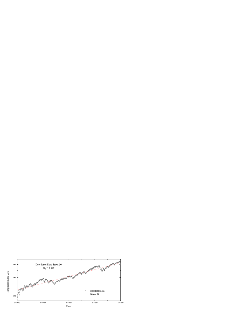
Figure 8: Logarithmic plot of Dow Jones Euro Stoxx 50 index $S(t)$ over $4$ years (5 Feb 2003 - 21 March 2007, in total $1057~{}$trading days) with sampling interval $\Delta t_{0}=1$ day. The index is fitted by a straight line, implying an exponential growth at an annual rate $\approx 20\%$.

 

The associated empirical option prices are plotted in Fig. 9. It is clear that because of the noise in the data no option pricing formula will fit the market prices perfectly.

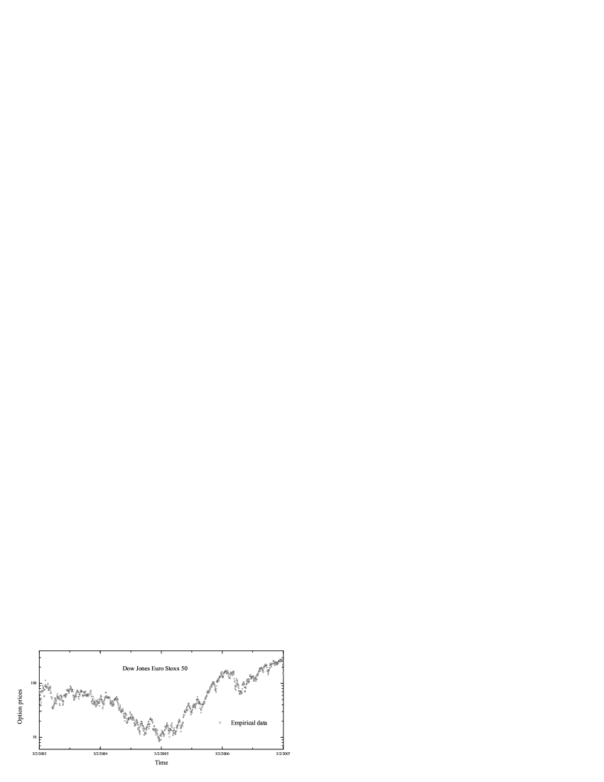
Figure 9: Option prices for an European option with a strike price $4200~{}$EUR and expiry on 21 December 2007. The underlying of the option is the Dow Jones Euro Stoxx 50 with the time series given in Fig. 8.

 

Even for a very good fit the option price would not be the most meaningful measure for the quality of the pricing model. Instead, one should test directly the hedging qualities of the pricing model B-P . To this end one introduces the $\Delta$-hedge

$$\Delta(\tau)\ \equiv\ \frac{\partial O_{\delta}(\tau)}{\partial S(\tau)}\,.$$ (78)

Given $\Delta(\tau)$ we construct a so-called $\Delta$-hedged portfolio $\Pi(\tau)$ by mixing stocks and options so that

$$\Pi(\tau)=O_{\delta}(\tau)-\Delta(\tau)S(\tau)\,.$$ (79)

The cash amount $\Pi$ can be interpreted as the value of a portfolio of a trader who at time $\tau$ bought one option $O_{\delta}(\tau)$ and sold an amount $\Delta(\tau)$ of the underlying with price $S(\tau)$. In the ideal situation, i.e., neglecting the time delays in the determination of $\Delta(\tau)$ and the adaptation of the portfolio, and ignoring the transaction costs, this portfolio is perfectly hedged, i.e., it is free of fluctuations since the fluctuations of $S$ and $O_{\delta}$ cancel each other B-P . The growth of the portfolio is therefore deterministic and proceeds at the riskfree rate $r_{W}$:

$$\frac{\textrm{d}\Pi(\tau)}{\textrm{d}\tau}\ =\ r_{W}\ \!\Pi(\tau)\,.$$ (80)

Any other growth rate would yield arbitrage possibilities. The amount $\Delta(\tau)$ deduced directly from empirical data should thus yield portfolio $\Pi(\tau)$ that is almost precisely $e^{r_{W}\tau}$ (modulo multiplicative pre-factor). Consequently, $\Delta(\tau)$ computed from a good option pricing formula must give $\Pi(\tau)$ that is also close to the $e^{r_{W}\tau}$ behavior. In our case the $\Delta$-hedge is

$$\Delta\ = \ \Phi^{(+)}_{v}(A)\ +\ \left[S\ \frac{\partial\Phi^{(+)}_{v}(A)}{\partial A}\ -\ Ee^{-r_{W}t}\ \frac{\partial\Phi^{(-)}_{v}(A)}{\partial A}\right]\frac{\textrm{d}A}{\textrm{d}S}\ =\ \Phi^{(+)}_{v}(A)\,,$$ (81)

since the expression in the square bracket vanishes due to Eqs. (58), (107) and the identities [see e.g., Ref. G-R ]

$$\frac{\partial\!~{}_{1\!}F_{1}(a,b,A)}{\partial A}\ =\ \frac{a}{b}\!~{}_{1\!}F_{1}(a+1,b+1,A)\,,$$ (82)

$$\!~{}_{1\!}F_{1}(a,b,A)\ =\ e^{A}\!~{}_{1\!}F_{1}(b-a,b,-A)\ =\ \frac{S}{E}\ \!e^{r_{W}t}\!~{}_{1\!}F_{1}(b-a,b,-A)\,,$$ (83)

$$a\ \!\!~{}_{1\!}F_{1}(a+1,b,A)\ =\ a\ \!\!~{}_{1\!}F_{1}(a,b,A)\ +\ A\ \!\frac{\partial\!~{}_{1\!}F_{1}(a,b,A)}{\partial A}\ \,.$$ (84)

Let us note that by comparing (79) with the option-pricing formula (33) we can write the portfolio at the time $\tau$ in the explicit form

$$\Pi(\tau)\ =\ -Ee^{-r_{W}(t_{b}-\tau)}\Phi^{(-)}_{v}(\tau)\,.$$ (85)

Imperfectness of the hedging induced by the pricing formula (33) thus depends on the actual behavior of $\Phi^{(-)}_{v}(\tau)$ in time. In the Black-Scholes model the corresponding $\Phi(y^{-}_{v})$ is effectively $\tau$-independent due to assumed form of the geometric Brownian motion for $S(\tau)$. In our model the situation is less obvious because the additional stochastic process due to volatility may substantially spoil the time independence. To see how big is the amount of the residual risk implied by our pricing model we turn now back to our empirical data. The best option-pricing solution $O_{\delta}$ fit for the empirical option-price data from Fig. 9 is depicted in Fig. 10. In the plot Fig. 10 (and the plots to follow) we have used $O_{\delta}$ calculated to $25$th perturbation order with the double-poles removed. The obtained result is quite robust with the residual error smaller that $0.05\%$.

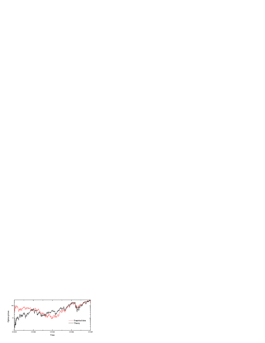
Figure 10: The best $O_{\delta}$ fit for the Dow Jones Euro Stoxx 50 option prices (cf. Fig. 9). On this scale the Black-Scholes solution basically coincides with the $O_{\delta}$ prediction.

 

Using as inputs: $E=4200~{}$EUR, $r_{W}=4.5$%/year and $t_{b}=1270~{}$trading days ($t_{a}=5~{}$Feb$~{}2003\equiv 0$), the corresponding free parameters are then best fitted with $\delta=69.43$, $\mu=351.29$ (i.e., $\bar{v}=0.000041$). The fit can be further optimized when newly arrived option pricing data are taken into account. Details of the departure of the $O_{\delta}$ prediction from the Black-Scholes fit is depicted in Figs. 11.

​​​​​​​​​​​​​​​​​​​​​

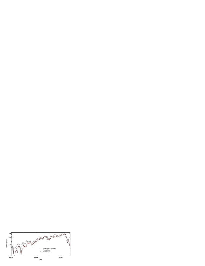
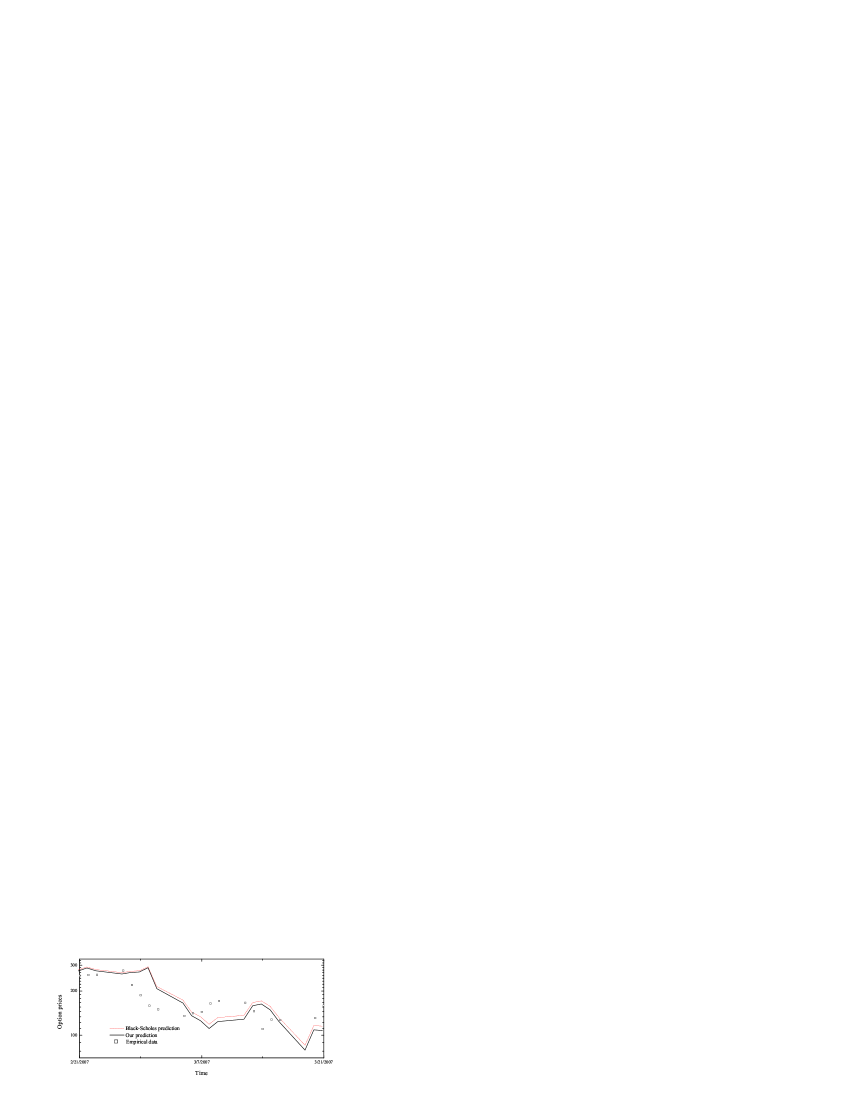
Figure 11: Two successive details of the departure of the $O_{\delta}$ fit from the Black-Scholes values. Black-Scholes option prices are taken with $v\equiv\overline{v}$. The roughly $5\%$ departure is clearly visible already $9-10$ months before the expiry date.

 

The goodness of the fit can be estimated, for instance, by the method of least squares. The correspondent likelihood function $\chi^{2}$ is for the $O_{\delta}$ fit in the period $21~{}$Dec$~{}006-21~{}$Jan$~{}2007$ smaller by $1.2\%$ in comparison with the Black-Scholes best fit. In the period $21~{}$Jan$~{}2007-21~{}$Feb$~{}2007$ the difference in $\chi^{2}$ is $1.8\%$, and in the period $21~{}$Feb$~{}2007-21~{}$Mar$~{}2007$ it is already $3.3\%$. This trend seems to get even more pronounced for periods closer to the expiry date.

According to Section V, the characteristic time corresponds to the time scale where non-Gaussian effects begin to smear out and beyond which the CLT begins to operate. For the call options at hand $t^{*}=3\delta\sim 210$ days, which, is particularly large and although the actual value will get further adjust with newly arrived option data, Fig. 11 indicates that $t^{*}$ will not get dramatically changed. Note also, that despite the fact that $t^{*}=210$ days, the departure effect is visible already $10$ months before the maturity.

By having the best $O_{\delta}$ fit we can construct the daily portfolio $\Pi$ according the prescription (79). The resulting portfolio is shown in Fig. 12.

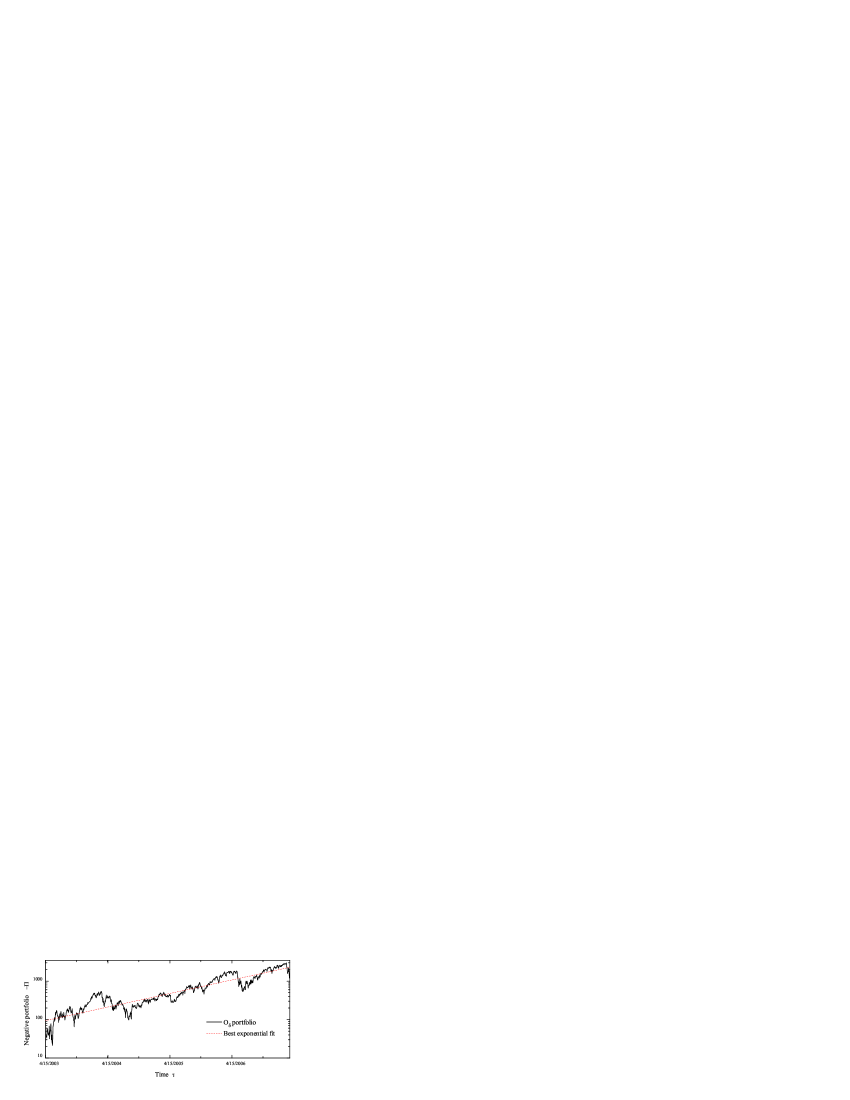
Figure 12: Negative daily portfolio $-\Pi$ constructed from the $O_{\delta}$ pricing formula (33) through $\Delta$-hedging prescription (78) and (79). The best exponential fit confirms the annual interest rate $4.5\%$. The relative fluctuations $\delta r_{W}(\tau)/r_{W}=0.007\pm 0.002$.

 

To quantify the fluctuations it is convenient to write $\Pi(\tau)=-E\Phi^{(-)}_{v}(\tau)\ \!e^{-(t_{b}-\tau)r_{W}}=-E\Phi(y^{-}_{v})\ \!e^{-(t_{b}-\tau)(r_{W}+\delta r_{W}(\tau))}$. The relative interest-rate fluctuations $\delta r_{W}/r_{W}$ implied by the stochastic nature of the volatility are according to Fig. 12, $0.007(\pm 0.002)$. Consequently we can conclude that for the data at hand the $O_{\delta}$ pricing formula induces a $\Delta$-hedging strategy that is close to being optimal.

VII Conclusions and Outlook

We have developed the theory of an option pricing model with a stochastic volatility following a Chi distribution. The corresponding volatility variance is then distributed with an ubiquitous Gamma distribution. Our direct motivation was drawn from the high-frequency S&P 500 volatility fluctuation data, whose distribution is well fitted in this way. There are two interesting implications resulting from such volatility fluctuations. First, the returns of the corresponding asset prices exhibit semi-heavy tails around the peak (i.e., leptocurtic behavior) which mimics empirically observed long-range correlations. At the same time, the returns preserve some of typical features of the original Black-Scholes model, namely they follow a linear Itō stochastic equation with multiplicative noise (though with stochastic volatility) and a continuous stock dynamics. Second, the associated density operator in momentum space is of the Tsallis type. The inverse Tsallis temperature then agrees with the average variance of the distribution.

Our main result is a generalized Black-Scholes pricing formula that takes into account the above volatility behavior. With the help of a Mellin transform we were able to find an ensuing analytic solution for the price of European call options. The result is expressed as a series in the higher normalized cumulants and in higher moments of moneyness. Due to a spread parameter $\delta$ related to the extra kurtosis of the log-return data, our model is capable of calibration to a richer set of observed market histories than the simple Black-Scholes model, which is a special case corresponding to a zero spread $\delta$, or to a very long time horizon ($t\gg t^{*}\sim\delta$). Comparisons with other time-dependent volatility models such as ARCH Engle82 , GARCH Bollerslev86 or multiscale GARCH Z-L03 will be addressed in future work.

In the light of recent works on superstatistics we should mention that the density operator representation (15) reveals the superstatistic nature of the Tsallis distribution in momentum space. Recently, C. Beck 1 ; 2 and C. Beck and E. Cohen 3 , prompted by the works by G. Wilk and Z. Wlodarczyk 4 , have suggested that the origin of certain heavy-tail distributions should be understood as weighted averages of the usual exponential statistics. Such averages have been used also in the textbook HK to calculate option prices for non-Gaussian distributions REPI . Recently, F. Sattin 5 rephrased the same procedure in terms of evolving systems embedded within a static but non-trivial background. All these approaches commonly strive to interpret broad distributions as a result of an averaging of usual exponential (Gibbs) distributions over certain fluctuating (random) parameter. This is the procedure running under the name superstatistics 3 ; 5 . Although frequently used, superstatistics procedure is still far from being systematized and, in fact, smearing distributions are usually chosen to fit experimental data. The theory of option pricing in this work may therefore be viewed as an example for superstatistics with a smeared Gaussian representing the probability distribution of volatilities.

Finally, the present scenario also provides an interesting meaning to the Tsallis escort parameter $q$. In option pricing models where stock fluctuations are directly fitted by a Tsallis distribution of returns HK ; Borland , the $q$ parameter is a fit parameter with a typical value around $1.5$. In the present case where the momentum distribution is of the Tsallis type, $q-1$ is proportional to the characteristic time $t^{*}$ below which the Gaussian treatment of stock fluctuations is inadequate.

Appendix A Fokker-Planck equation for stochastic Eq.(1) and some consequences

Some remarks may be useful concerning the stochastic equations for volatility and variance stated in the introduction.

Let us assume that the variance $v$ is driven by the Itō stochastic process

$$\textrm{d}v(t)\ =\ \gamma(t)[\nu(t)-\mu(t)v(t)-a(v(t),\mu(t),\nu(t))]\textrm{d}t\ +\ \sqrt{2\gamma(t)v(t)}\;\!\textrm{d}W(t)\,.$$ (86)

Here $\gamma(t),\mu(t)$ and $\nu(t)$ are arbitrary non-singular positive real functions on $\mathbb{{R}}^{+}$. The function $a(v(t),\mu(t),\nu(t))$ is assumed to be a non-singular function of its arguments. The corresponding Fokker-Planck equation for the distribution function $\rho(v,t)$ reads

$$\frac{\partial\rho(v,t)}{\partial t}\ =\ \frac{\partial}{\partial v}\left\{\gamma(t)\left[v\mu(t)-\nu(t)+a(v,\mu(t),\nu(t))\right]\,\!\rho(v,t)\right\}\ +\ \frac{\partial^{2}}{\partial v^{2}}\left[\gamma(t)v\,\!\rho(v,t)\right]\,.$$ (87)

Let us choose the function $a(v,\mu(t),\nu(t))$ to be

$$a(v,\mu,\nu)\ =\ v\frac{(\log\mu)^{\prime}}{\gamma}\ + \ ve^{v\mu}\left\{\left[\Gamma(\nu)\log\left(\frac{v\mu}{\nu}\right)+\Gamma(\nu,v\mu)(\psi(\nu)-\log(v\mu))\right](v\mu)^{-\nu}\right.$$ (88)

$$- \left.\frac{~{}_{2}F_{2}(\nu,\nu;\nu+1,\nu+1;-v\mu)}{\nu^{2}}\right\}\frac{(\nu)^{\prime}}{\gamma}\,,$$

where $\Gamma(x,y)$ is the incomplete gamma function, $\psi(x)$ the digamma function, and $\!\!~{}_{2}F_{2}$ a hypergeometric function G-R ) the solution of (87) has the form

$$\rho(v,t)\ =\frac{1}{\Gamma(\nu(t))}~{}[\mu(t)]^{\nu(t)}v^{\nu(t)-1}e^{-\mu(t)v}\,.$$ (89)

This is precisely the Gamma distribution $f_{\mu(t),\nu(t)}(v)$ in Eq. (2) describing the temporal statistical evolution of the random variable $v$. Note also that $\gamma(t)$ does not enter in the solution.

By applying the Itō formula of the stochastic calculus BO1 one easily obtains the corresponding Itō stochastic equation for the volatility $\sigma=\sqrt{v}$ in the form

$$\textrm{d}\sigma(t)\ =\ \frac{\gamma(t)}{2}\left[\frac{(\nu(t)-1/2)}{\sigma(t)}-\mu(t)\sigma(t)-\frac{a(\sigma^{2}(t),\mu(t),\nu(t))}{\sigma(t)}\right]\textrm{d}t\ +\ \sqrt{\frac{\gamma(t)}{2}}\;\!\textrm{d}W(t)\,,$$ (90)

from which we derive the Fokker-Planck equation for the distribution of the volatility $\sigma=\sqrt{v}$:

$$\frac{\partial\rho(\sigma,t)}{\partial t}\ = \ \frac{\partial}{\partial\sigma}\left\{\frac{\gamma(t)}{2}\left[\sigma\mu(t)-\frac{(\nu(t)-1/2)}{\sigma}+\frac{a(\sigma^{2},\mu(t),\nu(t))}{\sigma}\right]\,\!\rho(\sigma,t)\right\}$$ (91)

$$+ \ \frac{\partial^{2}}{\partial\sigma^{2}}\left[\frac{\gamma(t)}{4}\,\!\rho(\sigma,t)\right].$$

Of course, this equation is simply related to (87) by the substitution $v=\sigma^{2}$. Equation Eq.(91) has the solution

$$\rho(\sigma,t)\ =\ 2\sigma f_{\mu(t),\nu(t)}(\sigma^{2})\,,$$ (92)

which is also known as the Chi distribution feller ; wik .

The particular solutions (89) and (92) are the only ones fulfilling the asymptotic conditions $\rho(v,t)|_{t\rightarrow\infty}=\delta(v-\bar{v})$ and $\rho(\sigma,t)|_{t\rightarrow\infty}=\delta(\sigma-\bar{\sigma})$, respectively. They are also both normalized to unity. Note that the uniqueness of the solutions (89) and (92) ensures that the stochastic equations (86) and (91) have weak solutions.

Anticipating the empirical form presented in Section II we shall now assume that at large $t$ the functions $\mu(t)$ and $\nu(t)$ behave like $\mu(t)\approx\mu t$ and $\nu(t)\approx\nu t$. Without loss of generality we also set $\gamma(t)=1$. In this case the large-$t$ behavior of $a(v,\mu(t),\nu(t))$ can be easily found. Using the asymptotic formulas Luke

$$\psi(\nu t)|_{t\rightarrow\infty}\ \approx\ \log(\nu t)\,,$$

$$\!\!~{}_{2}F_{2}(\nu t,\nu t;\nu t+1,\nu t+1;-v\mu t)|_{t\rightarrow\infty}\ \approx\ e^{-v\mu t}\left(1\ +\ \frac{v\mu}{\nu}\right)^{\!2}\,,$$

$$\Gamma(\nu t,v\mu t)|_{t\rightarrow\infty}\ \approx\ e^{-\nu t}(\nu t)^{\nu t-1/2}\sqrt{2\pi}\ -\ (\nu t)^{-1}(v\mu t)^{\nu t}e^{-v\mu t}\left(1\ +\ \frac{v\mu}{\nu}\right)\,,$$ (93)

we obtain that $a(v,\mu(t),\nu(t))|_{t\rightarrow\infty}\ \approx\ {\mathcal{O}}(1/t)$. In this limit, the stochastic differential equation (86) for the variance corresponds to the Cox-Ingersoll-Ross process CIR . Although this asymptotic equation resembles Heston’s stochastic volatility model Heston1 , there is a difference: in the drift term $v(t)$ and $\mu(t)$ are linear functions of $t$ rather than constants.

Let us assume the same linear behavior $\mu(t)\approx\mu t$ and $\nu(t)\approx\nu t$ at small $t$ (more precisely for $\nu t\ll 1$). For convenience we set $\mu/\nu\equiv\overline{v}$, as in Section III. The small-$t$ behavior of $a(\ldots)$ can be easily found from the asymptotic formulas Luke

$$\psi(\nu t)|_{\nu t\rightarrow 0}\ \approx\ -\frac{1}{\nu t}+C\,,$$

$$\!\!~{}_{2}F_{2}(\nu t,\nu t;\nu t+1,\nu t+1;-v/\overline{v}\ \!\nu t)|_{\nu t\rightarrow 0}\ \approx\ 1\,,$$

$$\Gamma(\nu t,v/\overline{v}\ \!\nu t)|_{\nu t\rightarrow 0}\ \approx\ -\mbox{log}[\nu t]-\mbox{log}[v/\overline{v}]-C\,,$$ (94)

where $C=0.57731...$ is the Euler-Mascheroni constant. Then $a(v,\mu(t),\nu(t))|_{\nu t\rightarrow 0}\ \approx\ -v/(\overline{v}\ \!t\nu)+{\mathcal{O}}(1/\nu t)$. This shows that in the small-$t$ limit, the drift term is dominated by the function $a(v,\mu(t),\nu(t))$. Let us finally note that the stochastic equation (90) corresponds to an additive process, rather than to a multiplicative one.

Appendix B Calculation of $\Phi^{(-)}_{v}$

Let us calculate the function $\Phi^{(-)}_{v}$in Eq. (64) appearing in the generalized Black-Scholes formula (33). The procedure is analogous to that for $\Phi^{(+)}_{v}$. We start from Eq. (37) which reads now

$$\Phi^{(-)}_{v}~{} = ~{}\frac{1}{2}~{}+~{}{{\cal P}}\int_{-\infty}^{\infty}\frac{\textrm{d}p}{2\pi i}~{}F^{(-)}_{t\mu,t/\delta}(p)~{}\frac{e^{-p^{2}/2}}{p}\,,$$ (95)

where

$$F^{(-)}_{t\mu,t/\delta}(p)\ = \ 2\frac{\mu^{t/\delta}}{\Gamma(t/\delta)}\int_{0}^{\infty}\textrm{d}\omega\ \omega^{2t/\delta-1}~{}e^{-\mu\omega^{2}}\ \exp\left[i\frac{p}{2}\left(\frac{2A}{\omega}-\omega\right)\right]$$ (96)

$$\equiv \ 2\frac{\mu^{t/\delta}}{\Gamma(t/\delta)}~{}g^{(-)}_{\mu}(p,A)~{},$$

To find $g^{(-)}_{\mu}(p,A)$ we first calculate the integral

$$\int_{0}^{\infty}\textrm{d}\mu~{}\mu^{s-1}g^{(-)}_{\mu}(p,A)~{} = ~{}\Gamma(s)\int_{0}^{\infty}\textrm{d}\omega~{}\omega^{2t/\delta-2s-1}\ \exp\left[i\frac{p}{2}\left(\frac{2A}{\omega}-\omega\right)\right]$$ (97)

$$= ~{}\Gamma(s)(2A)^{t/\delta-s}\int_{-\infty}^{\infty}\textrm{d}u\ e^{-ip\sqrt{2A}\cosh u-(2s-2t/\delta)u}$$

$$= ~{}2\Gamma(s)(e^{-i\pi}2A)^{t/\delta-s}K_{2s-2t/\delta}(p\sqrt{2A})\,,\;\;\;\;\;\;\;(p>0)\,,$$

where $K_{\alpha}(z)$ is the modified Bessel function Watson . The result (97) holds in a strip $t/\delta-1/2<{\Re}(s)<t/\delta+1/2$. Similar calculations for $p<0$ yields

$$\int_{0}^{\infty}\textrm{d}\mu~{}\mu^{s-1}g^{(-)}_{\mu}(p,A)~{} = \ 2\Gamma(s)(e^{i\pi}2A)^{t/\delta-s}K_{2s-2t/\delta}(-p\sqrt{2A})\,,\;\;\;\;\;\;\;(p<0)\,.$$ (98)

Again, the result is true in a strip $t/\delta-1/2<{\Re}(s)<t/\delta+1/2$. With the help of the Mellin inverse transform we now find

$$g^{(-)}_{\mu}(p,A)~{}=~{}\int_{c-i\infty}^{c+i\infty}\frac{\textrm{d}s}{2\pi i}\ 2\mu^{-s}\Gamma(s)\!\left\{\begin{array}[]{l}(e^{-i\pi}2A)^{t/\delta-s}K_{2s-2t/\delta}(p\sqrt{2A}),~{}~{}~{}p>0.\\[5.69054pt] (e^{i\pi}2A)^{t/\delta-s}K_{2s-2t/\delta}(-p\sqrt{2A}),~{}~{}~{}p<0,\end{array}\right\}$$ (101)

where $c\in(t/\delta-1/2,t/\delta+1/2)$. Inserting this back into (96) and (95) we obtain

$$\Phi^{(-)}_{v} = \frac{1}{2}+\frac{2\mu^{t/\delta}}{\Gamma(t/\delta)}\ \!{{\cal P}}\!\!\int_{-\infty}^{\infty}\frac{\textrm{d}p}{2\pi i}\frac{e^{-p^{2}/2}}{p}\int_{c-i\infty}^{c+i\infty}\!\!\frac{\textrm{d}s}{\pi i}~{}\mu^{-s}\Gamma(s)\!\left\{\begin{array}[]{l}(e^{-i\pi}2A)^{t/\delta-s}K_{2s-2t/\delta}(p\sqrt{2A})\\[5.69054pt] (e^{i\pi}2A)^{t/\delta-s}K_{2s-2t/\delta}(-p\sqrt{2A})\end{array}\right\}$$ (104)

$$= \!\!\!\!\!\!\!\frac{1}{2}+\frac{4}{\Gamma(t/\delta)}\int_{c-i\infty}^{c+i\infty}\!\!\frac{\textrm{d}s}{2\pi i}~{}\Gamma(s)(2A\mu)^{t/\delta-s}\sin[\pi(s-t/\delta)]\int_{0_{+}}^{\infty}\frac{\textrm{d}q}{\pi}\frac{e^{-p^{2}/2}}{p}K_{2s-2t/\delta}(p\sqrt{2A})\,.$$

The $p$-integration can be carried out explicitly yielding ($\zeta\equiv s-t/\delta$)

$$\mbox{}\sin(\pi\zeta)\int_{0_{+}}^{\infty}\textrm{d}p~{}\frac{e^{-p^{2}/2}}{p}\ K_{2\zeta}(p\sqrt{2A})$$

$$\mbox{}=\ \frac{\sin(\pi\zeta)}{4}\left[A^{-\zeta}\Gamma(-\zeta)\Gamma(2\zeta)~{}_{1\!}F_{1}(-\zeta,1-2\zeta,A)+A^{\zeta}\Gamma(\zeta)\Gamma(-2\zeta)~{}_{1\!}F_{1}(\zeta,1+2\zeta,A)\right]$$

$$\mbox{}=~{}-\frac{\sqrt{\pi}}{8\zeta}\left[\!\left(\frac{A}{4}\right)^{\!\!\zeta}\Gamma\!\left(\mbox{ $\!\!\frac{1}{2}$}-\zeta\right)\!\!~{}_{1\!}F_{1}(\zeta,1+2\zeta,A)+\left(\frac{A}{4}\right)^{\!\!-\zeta}\Gamma\!\left(\zeta+\mbox{ $\!\!\frac{1}{2}$}\right)\!\!~{}_{1\!}F_{1}(-\zeta,1-2\zeta,A)\right].$$ (106)

The integration is valid for $\Re~{}\zeta>0$ and $\Re~{}\zeta<0$. The result allows us to write $\Phi^{(-)}_{v}$ as

$$\Phi^{(-)}_{v}~{}=~{}\frac{1}{2}~{}-~{}h^{(-)}_{1}(\mu,t/\delta,A)~{}-\ h^{(-)}_{2}(\mu,t/\delta,A)\,,$$ (107)

with

$$h^{(-)}_{1}(\mu,t/\delta,A)~{} = \ \frac{1}{2\Gamma(t/\delta)\sqrt{\pi}}~{}\sum_{\mathrm{Res}}\frac{\Gamma(\zeta+t/\delta)}{\zeta}\left(8\mu\right)^{-\zeta}\Gamma\!\left(\mbox{ $\!\!\frac{1}{2}$}-\zeta\right)\!~{}_{1\!}F_{1}(\zeta,1+2\zeta,A)\,,$$

$$h^{(-)}_{2}(\mu,t/\delta,A)~{} = \ \frac{1}{2\Gamma(t/\delta)\sqrt{\pi}}~{}\sum_{\mathrm{Res}}\frac{\Gamma(\zeta+t/\delta)}{{\zeta}}\left(\frac{A^{2}\mu}{2}\right)^{-\zeta}\Gamma\!\left(\zeta+\mbox{ $\!\!\frac{1}{2}$}\right)\!~{}_{1\!}F_{1}(-\zeta,1-2\zeta,A)\,.$$

Mellin’s fundamental strip for $\zeta$ can be conveniently chosen in $h^{(-)}_{1}$ as $0<\zeta<1/2$, and in $h^{(-)}_{2}$ as $-1/2<\zeta<0$. As previously in the calculation of $\Phi^{(+)}_{v}$, the contour of the $s$-integration for $h^{(-)}_{2}$ is closed on the left. Thus we obtain by analogy with $\Phi^{(+)}_{v}$ that the final expression has the form (64).

In the small-$\delta$ limit where $(t/\delta)_{z}\rightarrow(t/\delta)^{z}$, the third sum in (64) goes to zero. In such a situation

$$\Phi^{(-)}_{v}~{}=~{}\frac{1}{2}\left[1~{}+~{}\sqrt{\frac{2}{\pi}}~{}y_{\bar{v}}^{-}\!~{}_{1\!}F_{1}\left(\frac{1}{2},\frac{3}{2},-\frac{\left(y_{\bar{v}}^{-}\right)^{2}}{2}\right)\right]~{}=~{}\Phi(y_{\bar{v}}^{-})\,,$$ (109)

i.e., we regain the cumulative normal distribution. In the limit $A\rightarrow 0$, one finds that $\Phi^{(-)}_{v}\rightarrow\Phi(y_{\bar{v}}^{-})|_{A=0}$.

Appendix C: Information Entropy and Tsallis Statistics

A useful conceptual frame that allows to generate important classes of distributions is based on information entropies. Information entropies generally represent measures of uncertainty inherent in a distribution describing a given statistical or information-theoretical system. Central role of information entropies is in that they serve as inference functionals whose extremalization subject to certain constraint conditions (known as prior information), yields the MaxEnt distribution. Importance of information entropies as tools for inductive inference (i.e., inference where new information is given in terms of expected values) was emphasized by many authors Fad1 .

Among the many possible information entropies one may focus attention on two examples, first on Rényi’s entropy

$${\mathcal{S}}_{q}^{(R)}~{}=~{}\frac{1}{1-q}\log\sum_{i}p_{i}^{q}\,,\;\;\;\;\;\;\;\;q>0\,,$$ (110)

and second on the Tsallis-Havrda-Charvát (THC) entropy

$${\mathcal{S}}_{q}^{(THC)}~{}=~{}\frac{1}{1-q}\left(\sum_{i}p_{i}^{q}-1\right)\,,\;\;\;\;\;\;\;\;q>0\,.$$ (111)

The discrete distribution ${\mathcal{P}}=\{p_{i}\}$ is usually associated with a discrete set of micro-states in statistical physics, or set of all transmittable messages in information theory. In the limit $q\rightarrow 1$, the two entropies coincide with each other, both reducing to the thermodynamic Shannon-Gibbs entropy

$$S~{}=~{}-\sum_{i}p_{i}\log p_{i}\,.$$ (112)

Thus the parameter $q-1$ characterizes the departure from the usual Boltzmann-Gibbs statistics or from Shannonian information theory.

It is well known jaynes57 that within the context of Shannonian information theory the laws of equilibrium statistical mechanics can be viewed as inferences based entirely on prior information that is given in terms of expected values of energy and number of particles, energy and volume, energy and angular momentum, etc. For the sake of simplicity we shall consider here only the analog of canonical ensembles, where the prior information is characterized by a fixed energy expectation value. The corresponding MaxEnt distributions for ${\mathcal{S}}_{q}^{(R)}$ and ${\mathcal{S}}_{q}^{(THC)}$ can be obtained by extremizing the associated inference functionals

$$L_{q}^{(R)}({\mathcal{P}})~{} = ~{}\frac{1}{1-q}\log\sum_{i}p_{i}^{q}~{}-~{}\alpha\sum_{i}p_{i}~{}-~{}\beta\langle H\rangle_{r}\,,$$

$$L_{q}^{(THC)}({\mathcal{P}})~{} = ~{}\frac{1}{1-q}\left(\sum_{i}p_{i}^{q}-1\right)~{}-~{}\alpha\sum_{i}p_{i}~{}-~{}\beta\langle H\rangle_{r}\,,$$ (113)

where $\alpha$ and $\beta$ are Lagrange multipliers, the latter being the analog of the inverse temperature in natural units. The subscript $r$ on the energy expectation value $\langle H\rangle$ distinguishes two conceptually different approaches. In information theory one typically uses the linear mean, i.e.,

$$\langle H\rangle_{1}~{}\equiv~{}\langle H\rangle_{r=1}~{}=~{}\sum_{i}p_{i}E_{i}\,,$$ (114)

while in non-extensive thermostatistics it is customary to utilize a non-linear mean

$$\langle H\rangle_{q}~{}\equiv~{}\langle H\rangle_{r=q}~{}=~{}\sum_{i}P_{i}(q)E_{i},\,\;\;\;\;\mbox{with}\;\;\;\;P_{i}(q)~{}\equiv\ \frac{p_{i}^{q}}{\sum_{i}p_{i}^{q}}\,,\;\;\;\sum_{i}p_{i}~{}=~{}1\,.$$ (115)

The distribution $P_{i}(q)$ is called escort or zooming distribution and it has its origin in chaotic dynamics beck and in the physics of multifractals PJ1 . Simple analysis reveals 11 that

$$\frac{\delta L_{q}^{(R)}({\mathcal{P}})}{\delta p_{i}}~{}=~{}0\ \Rightarrow\left\{\begin{array}[]{ll}{p}_{i}^{(1)}~{}=~{}Z_{R}^{-1}\left[1~{}-~{}\tilde{\beta}(q-1)\Delta E_{i}\right]^{1/(q-1)},&\;\;{\mbox{for}}\;\;\langle H\rangle_{r=1}\,,\\[8.53581pt] p^{(2)}_{i}~{}=~{}Z_{R}^{-1}\left[1~{}-~{}\beta(1-q)\Delta E_{i}\right]^{1/(1-q)},&\;\;\hbox{for}\;\;\langle H\rangle_{r=q}\,.\end{array}\right.$$ (118)

Here $\tilde{\beta}=\beta/q$ and $\Delta E_{i}=E_{i}-\langle H\rangle_{r}$. By the same token one obtains for the THC case 11

$$\frac{\delta L_{q}^{(THC)}({\mathcal{P}})}{\delta p_{i}}~{}=~{}0\ \Rightarrow\left\{\begin{array}[]{ll}{p}^{(1)}_{i}~{}=~{}Z_{THC}^{-1}\left[1~{}-~{}\tilde{\beta}^{*}(q-1)\Delta E_{i}\right]^{1/(q-1)},&\;\;{\mbox{for}}\;\;\langle H\rangle_{r=1}\,,\\[8.53581pt] p^{(2)}_{i}~{}=~{}Z_{THC}^{-1}\left[1~{}-~{}\beta^{*}(1-q)\Delta E_{i}\right]^{1/(1-q)},&\;\;{\mbox{for}}\;\;\langle H\rangle_{r=q}\,,\end{array}\right.$$ (121)

with $\beta^{*}~{}=~{}\beta/\sum_{i}p_{i}^{q}$ and $\tilde{\beta}^{*}~{}=~{}\tilde{\beta}/\sum_{i}p_{i}^{q}$. So in contrast to (118), the THC MaxEnt distributions are self-referential. Generalized distributions of the form (118) and (121) are known as Tsallis distributions and they appear in numerous statistical systems Ts2a . For historical reasons is ${\mathcal{P}}^{(1)}=\{p_{i}^{(1)}\}$ in (121) also known as the Bashkirov’s $1$-st version of thermostatistics, while ${\mathcal{P}}^{(2)}=\{p_{i}^{(2)}\}$ in (121) is called the Tsallis’ $3$rd version of thermostatistics. An important feature of Tsallis distributions is that they are invariant under uniform shifts $\varepsilon$ of the energy spectrum. So one can always choose to work directly with $E_{i}$ rather than $\Delta E_{i}$.

References

- (1) S.L. Heston, A Closed-Form Solution for Options with Stochastic Volatility with Applications to Bond and Curren Options, Review of Financial Studies 6, 327 (1993).
- (2) R.F. Engle, Econometrica 50 (1982) 987
- (3) T. Bollerslev, J. Econometrics 31 (1986) 307
- (4) G. Zumbach and P. Lynch, Quantitative Finance 3 (2003) 320
- (5) E. Jacquier, N.G. Polson and P.E. Rossi, Journal of Business & Economic Statistics 12 (1994) 371
- (6) J.-P. Bouchaud and M. Potters, Theory of Financial Risks (Cambridge University Press, Cambridge, 2000)
- (7) J.-P. Bouchaud and D. Sornette, J. Phys. I (France) 4 (1994) 863 .
- (8) E.-F. Fama, J. Finance 25 (1970) 383
- (9) Z. Ding, C. W. J. Granger and R. F. Engle, J. Empirical Finance 1 (1993) 83
- (10) M. M. Dacorogna, U. A. Muller, R. J. Nagler, R. B. Olsen and O. V. Pictet, J. Int. Money and Finance 12 (1993) 413.
- (11) Y. Liu, P. Cizeau, M. Meyer, C.-K. Peng, and H.E. Stanley, Physica A 245 (1997) 437; Physica A 245 441; Y. Liu, P. Gopikrishnan, P. Cizeau, M. Mayer, C.-K. Peng and H.E. Stanley, Phys. Rev. E 60 (1999) 1390
- (12) H. Kleinert and X.J. Chen, Boltzmann Distribution and Market Temperature, Physica A to be published [physics/0609209]
- (13) A. Bunde and S. Havlin, in Fractals and Disordered Systems, ed. by A. Bunde and S. Havlin, ed., (Springer, Heidelberg 1996)
- (14) W. Feller, An Introduction to Probability Theory and Its Applications, Vol. II (John Wiley, London, 1966)
- (15) http://en.wikipedia.org/wiki/Chidistribution
- (16) H. Kleinert, Path Integrals in Quantum Mechanics, Statistics, Polymer Physics and Financial Markets, 4th ed. (World Scientific, Singapore 2006) (online at www.physik.fu-berlin.de/~kleinert/b5).
- (17) see e.g., R. Kubo, M. Toda and N. Hashitsume, Statistical Physics II: Nonequilibrium Statistical Mechanics (Springer, New York, 1995))
- (18) see, e.g., L. Borland, Phys. Rev. Lett. 89 (2002) 098701, Quantitative Finance 2 (2002) 415
- (19) F. Corsi, G. Zumbach, U.A. Muller and M.M. Dacorogna, Economic Notes 30 (2001) 183; M. Pasquini and M. Serva, Econophysics Letters, 65 (1999) 275; A. Pagan, J. Empirical Financa 3 (1996) 15; B. Zhou, Journal of Business & Economical Statistics 14 (1996) 45
- (20) J. Beran, Statistics for Long-Memory Processes (Chapman & Hall, New York, 1994)
- (21) M. Potters, R. Cont and J.-P. Bouchaud, [cond-mat/9609172]
- (22) A. Admati adn P. Pfleiderer, Rev. Financial Studies 1 (1988) 3
- (23) compare Eq. (20.144) and (20.145) in the textbook HK
- (24) see Subsection 20.5.4 of the textbook HK
- (25) European call options are options that give the right to purchase a unit of stock for a strike price only at expiration date.
- (26) see Subsection 20.5.5 of the textbook HK for this procedure
- (27) G.N. Watson, A Treatise on the Theory of Bessel Functions, 2nd ed., (Cambridge Un. Press, Cambridge, 1966)
- (28) H. Buchholz, The Confluent Hypergeometric Function with Special Emphasis on its Applications, (Springer-Verlag, New York, 1969)
- (29) Y.L. Luke, The Special Functions and their Approximations (Academic Press, London, 1969)
- (30) L.G. McMillan, Options as a Strategic Investment, 4th ed. (New York Institute of Finance, New York, 2002)
- (31) I.S. Gradshteyn, I.M. Ryzhik and A. Jeffrey (Eds.) Table of Integrals, Series and Products (Academic Press, San Diego, 1994)
- (32) B.V. Gnedenko and A.N. Kolmogorov, Limit Distributions for Sums of Independent Random Variables (Addison Wesley, Cambridge, MA., 1954)
- (33) C. Beck, Phys. Rev. Lett. 87 (2001) 180601
- (34) C. Beck, [cond-mat/0303288]
- (35) C. Beck and E.G.D. Cohen, Physica A 322 (2003) 267
- (36) G. Wilk and Z. Wlodarczyk, Phys. Rev. Lett. 84 (2000) 2770
- (37) F. Sattin, Physica A 338 (2004) 437
- (38) J.C. Cox, J.E. Ingersol and S. Ross, Econometrica 53 (1985) 373
- (39) B. Øksendal, Stochastic Differential Equations, An Introduction with Applications (Springer-Verlag, Berlin, 2003)
- (40) D.K Faddeyev, Uspekhi Mat. Nauk, 11 (1956); J.E. Shore and R.W. Johnson, IEEE Trans. Inform. Theory 26 (1980) 26.; in, E.T. Jaynes, Probability Theory, The Logic of Science (Cambridge Un. Press, Cambridge, 2003); F. Topsøe, Kybernetika 15 (1979) 8; IEEE Trans. Inform. Theory 48 (2002) 2368.
- (41) E.T. Jaynes, Phys. Rev. 106 (1957) 171; 108(1957) 620
- (42) C. Beck and F. Schlögl, Thermodynamics of chaotic systems: An introduction (Cambridge University Press, Cambridge, 1993)
- (43) P. Jizba and T. Arimitsu, Annals of Phys. (NY) 312 (2004) 17
- (44) A.G. Bashkirov, [cond-mat/0310211]; A.G. Bashkirov and A.D. Sukhanov, JETP 95 (2002) 440
-
(45)
see e.g., S. Abe and Y. Okamoto (Eds.), Nonextensive Statistical
Mechanicsand Its Applications (Springer-Verlag, New York, 2001) and
monographs in
http://tsallis.cat.cbpf.br/biblio.htm;
http://www.cbpf.br/GrupPesq/StatisticalPhys/books.htm