Velocity fluctuations in a one dimensional Inelastic Maxwell model.

Abstract

We consider the velocity fluctuations of a system of particles described by the Inelastic Maxwell Model. The present work extends the methods, previously employed to obtain the one-particle velocity distribution function, to the study of the two particle correlations. Results regarding both the homogeneous cooling process and the steady state driven regime are presented. In particular we obtain the form of the pair correlation function in the scaling region of the homogeneous cooling process and show that some of its moments diverge. This fact has repercussions on the behavior of the energy fluctuations of the model.

1 Introduction

In recent years the understanding of the physics of granular materials has taken great strides. The dynamical properties of particles experiencing mutual inelastic collisions has been thoroughly studied experimentally, theoretically and by computer simulation. Such an effort has lead to the discovery and to the formulation of new phenomena and properties [1]. Among these properties a special place is occupied by the homogeneous cooling state (HCS), i.e. the state achieved by a granular gas, initially in motion, under the effect of the energy loss caused by inelastic collisions. Loosely speaking the HCS plays for granular gases a role analogous to the Maxwellian for molecular elastic gases. Although the properties of the HCS are known in detail, its explicit form can be obtained as series expansion only for some specific models such as the inelastic hard-sphere model (IHS) [2].

The prototype model for the study of granular systems is represented by an assembly of smooth inelastic hard spheres, characterized by a constant coefficient of normal restitution. For such a model various authors have derived the Boltzmann and the Boltzmann-Enskog equations describing the evolution of the reduced one-particle velocity distribution [3]. However, since these approaches remain mathematically hard to solve, a simpler mathematical model, the Inelastic Maxwell Model (IMM), where the collision rate between the particles is assumed to be independent of the relative velocity of the colliding pair, has been put forward. In this model the spatial structure is neglected and only the velocity of the particles specifies the state of the system. The IMM is nevertheless useful and studied because it lends itself to analytical solution in one dimension, thus providing a benchmark to test approximate treatments [4]. In the homogeneous free cooling case [5], the evolution equation for the velocity distribution has a scaling solution that can be expressed in an analytical closed form, with high energy tails described by an algebraic decay: the exponent does not depend on the restitution coefficient. Moments of the velocity distribution exhibit multiscaling asymptotic behavior [6]. The Inelastic Maxwell Model is quite simplified with respect to inelastic hard spheres and other realistic models of dilute granular materials, nevertheless in the past it has been considered an important starting point for granular kinetic theories [7]. As stated by Ernst and Brito [8]: “What harmonic oscillators are for quantum mechanics, and dumb-bells for polymer physics, is what elastic and inelastic Maxwell models are for kinetic theory.”

Most of the literature on the kinetic theory of granular gases focuses on the single particle distribution function. This is in analogy with the relevance that the Molecular Chaos approximation has for molecular (i.e. elastic) gases. On the other hand, the inelasticity of collisions in granular gases makes this assumption more delicate: numerical and experimental evidences show a stronger tendency of granular systems to enhance correlations, often appearing in the form of spatial structures [9, 10, 11]. Fluctuations have been investigated by various authors [12, 13, 14]. However, only recently the two-particles distribution function has come under scrutiny, in particular by Brey and coworkers who considered its application to the study of the energy fluctuation in the homogeneous cooling state of inelastic hard spheres [15]. Their study focuses on the effect of inelasticity on the $1/N$ deviations from Molecular Chaos. Here, our aim is to apply similar analysis to the one dimensional Inelastic Maxwell Model. This is interesting because, with a few controlled approximations, one obtains the asymptotic pair correlation function in a closed form, and all time dependencies of its two-particles velocity moments, getting further than the original work of Brey et al., where only the asymptotic moments, in particular those required to calculate energy fluctuations, were explicitly obtained.

This paper is organized as follows. In section 2 the evolution equation for the IMM is presented and the equations for the various distribution functions introduced. In section 3 the dynamical equations are solved for the moments of the single and two-particles distribution functions. The asymptotic scaling state is discussed, for the pair correlation function, in section 4 . Finally, in Section 5 the effects of an external driving is considered and in 6 the concluding remarks are presented.

2 Evolution equations for the distribution functions

We consider a system of N particles, each characterized by a scalar velocity $v_{i}$, with $i=1,...,N$. The Inelastic Maxwell Model assumes that the state $\Gamma=(v_{1},v_{2},..,v_{N})$ is modified by elementary collision events, realized by changing the velocities $(v_{i},v_{j})$ of a randomly selected pair of particles according to the rule:

$$v_{i}^{\prime} = \gamma v_{i}+(1-\gamma)v_{j}$$ (1)

$$v_{j}^{\prime} = (1-\gamma)v_{i}+\gamma v_{j}\qquad$$

where $\gamma=\frac{1-\alpha}{2}$ and $\alpha$ is the coefficient of restitution. The system cools down because in each collision an amount $\Delta E$ of kinetic energy, given by

$$\Delta E=-\frac{m}{4}(1-\alpha^{2})(v_{i}^{\prime}-v_{j}^{\prime})^{2},\qquad$$ (2)

is dissipated, where $m$ is the mass of a particle. Since the IMM is not endowed with a spatial structure such a cooling process is homogeneous. An observable $A(\Gamma(t))$ evolves according to

$$A(\Gamma(t))=\exp(t{\cal L}A(\Gamma(0)))$$ (3)

where the generator ${\cal L}$ is

$${\cal L}=\frac{1}{2}\sum_{i=1}^{N}\sum_{j\neq i}^{N}T(v_{i},v_{j})$$ (4)

and the operator $T$ acts on an arbitrary function $S(v_{i},v_{j})$ of the velocities of particles $i$ and $j$ in the following way:

$$T(v_{i},v_{j})S(v_{i},v_{j})=S(v_{i}^{\prime},v_{j}^{\prime})-S(v_{i},v_{j})$$ (5)

The “time” $t$ is a collision counter and represents the clock of the model.

Following closely the derivation presented by Brey et al.[15], in order to set up the evolution equations for the system, we introduce the following distribution functions

$$F_{1}(u_{1},t)=\sum_{i=1}^{N}\langle\delta(u_{1}-v_{i}(t))\rangle$$ (6)

$$F_{2}(u_{1},u_{2},t)=\sum_{i=1}^{N}\sum_{j\neq i}^{N}\langle\delta(u_{1}-v_{i}(t))\delta(u_{2}-v_{j}(t))\rangle$$ (7)

$$F_{3}(u_{1},u_{2},u_{3},t)=\sum_{i=1}^{N}\sum_{j\neq i}^{N}\sum_{k\neq i,j}^{N}\langle\delta(u_{1}-v_{i}(t))\delta(u_{2}-v_{j}(t))\delta(u_{3}-v_{k}(t))\rangle$$ (8)

where $\langle\cdot\rangle$ stands for an average over an ensemble of trajectories with different initial conditions (in section 5, where the effect of a thermal bath will be considered, this will be an average over realizations of the noise).

A hierarchy of equations can be derived for these distribution functions, whose first two equations read:

$$\frac{d}{dt}F_{1}(u_{1},t)=\int du_{2}{\overline{T}}(u_{1},u_{2})F_{2}(u_{1},u_{2},t)$$ (9)

and

$$\frac{d}{dt}F_{2}(u_{1},u_{2},t) = {\overline{T}}(u_{1},u_{2})F_{2}(u_{1},u_{2},t)+$$ (10)

$$+ \int du_{3}[{\overline{T}}(u_{1},u_{3})+{\overline{T}}(u_{2},u_{3})]F_{3}(u_{1},u_{2},u_{3},t)$$

where the inverse binary collision operator, ${\overline{T}}$, is defined for a generic function $S(u_{i},u_{j})$ of the velocities by the rule:

$${\overline{T}}(u_{i},u_{j})S(u_{i},u_{j})=\frac{1}{\alpha}S(u_{i}^{*},u_{j}^{*})-S(u_{i},u_{j})$$ (11)

which transforms the velocities $(u_{i},u_{j})$ into their pre-collisional values $u_{i}^{*},u_{j}^{*}$, obtained by inverting eq. (1). Following a standard statistical procedure we consider the following decompositions of the distribution functions:

$$F_{2}(u_{1},u_{2},t)=F_{1}(u_{1},t)F_{1}(u_{2},t)+G_{2}(u_{1},u_{2},t)$$ (12)

$$F_{3}(u_{1},u_{2},u_{3},t) = F_{1}(u_{1},t)F_{1}(u_{2},t)F_{1}(u_{3},t)+G_{2}(u_{1},u_{2},t)F_{1}(u_{3},t)$$ (13)

$$+ G_{2}(u_{1},u_{3},t)F_{1}(u_{2},t)+G_{2}(u_{2},u_{3},t)F_{1}(u_{1},t)$$

$$+ G_{3}(u_{1},u_{2},u_{3},t)$$

After substituting these expressions into (9) and (10) and dropping the term containing $G_{3}$ we obtain a pair of closed equations for $F_{1}$ and $G_{2}$. Before proceeding further we also define, for later convenience, the following normalized distributions:

$$f_{1}(u_{1},t)=\frac{1}{N}F_{1}(u_{1},t)$$ (14)

and

$$h_{2}(u_{1},u_{2},t)=\frac{1}{N}G_{2}(u_{1},u_{2},t)$$ (15)

which obey the sum rules

$$\int du_{1}f_{1}(u_{1},t)=1$$ (16)

$$\int\int du_{1}du_{2}h_{2}(u_{1},u_{2},t)=-1$$ (17)

$$\int du_{2}h_{2}(u_{1},u_{2},t)=-f_{1}(u_{1},t)$$ (18)

Hence eqs. (9) and (10) can be rewritten as

$$\frac{d}{d\tau}f_{1}(u_{1},\tau)=\int du_{2}{\overline{T}}(u_{1},u_{2})[f_{1}(u_{1},\tau)f_{1}(u_{2},\tau)+\frac{1}{N}h_{2}(u_{1},u_{2},\tau)]$$ (19)

and

$$\frac{d}{d\tau} h_{2}(u_{1},u_{2},\tau)={\overline{T}}(u_{1},u_{2})[f_{1}(u_{1},t)f_{1}(u_{2},\tau)+\frac{1}{N}h_{2}(u_{1},u_{2},\tau)]$$ (20)

$$+ \int du_{3}{\overline{T}}(u_{1},u_{3})[h_{2}(u_{1},u_{2},\tau)f_{1}(u_{3},\tau)+h_{2}(u_{2},u_{3},t)f_{1}(u_{1},\tau)]$$

$$+ \int du_{3}{\overline{T}}(u_{2},u_{3})][h_{2}(u_{1},u_{2},\tau)f_{1}(u_{3},\tau)+h_{2}(u_{1},u_{3},\tau)f_{1}(u_{2},\tau)]$$

where we have redefined the time variable $\tau=Nt$.

In order to solve (19) and (20) we slightly generalize the method, originally introduced by Bobylev [16] and consider the following Fourier transforms of the distributions $f_{1}$ and $h_{2}$

$$\hat{f}_{1}(k_{1},t)=\int du_{1}e^{ik_{1}u_{1}}f_{1}(u_{1},t)$$ (21)

$$\hat{h}_{2}(k_{1},k_{2},t)=\int\int du_{1}du_{2}e^{ik_{1}u_{1}+ik_{2}u_{2}}h_{2}(u_{1},u_{2},t)$$ (22)

The function $\hat{h}_{2}(k_{1},k_{2},t)$ is symmetric and has the property $\hat{h}_{2}(k_{1},0,t)=-f_{1}(k_{1},t)$ as a consequence of the sum rule (18). Substituting these expressions into (19) and (20) we find:

$$\frac{d}{d\tau}\hat{f}_{1}(k_{1},\tau) = \hat{f}_{1}(\gamma k_{1},\tau)\hat{f}_{1}((1-\gamma)k_{1},\tau)-\hat{f}_{1}(k_{1},\tau)\hat{f}_{1}(0,\tau)$$ (23)

$$+ \frac{1}{N}[\hat{h}_{2}(\gamma k_{1},(1-\gamma)k_{1},\tau)-\hat{h}_{2}(k_{1},0,\tau)]$$

and

$$\frac{d}{d\tau} \hat{h}_{2}(k_{1},k_{2},\tau)=\frac{1}{N}[\hat{h}_{2}(\gamma k_{1}+(1-\gamma)k_{2},\gamma k_{2}+(1-\gamma)k_{1},\tau)-\hat{h}_{2}(k_{1},k_{2},\tau)]$$

$$+ \hat{f}_{1}(\gamma k_{1}+(1-\gamma)k_{2},\tau)\hat{f}_{1}(\gamma k_{2}+(1-\gamma)k_{1},\tau)-\hat{f}_{1}(k_{1},\tau)\hat{f}_{1}(k_{2},\tau)$$

$$+ (1+P_{12})[\hat{f}_{1}((1-\gamma)k_{1},\tau)\hat{h}_{2}(\gamma k_{1},k_{2},\tau)-\hat{f}_{1}(0,\tau)\hat{h}_{2}(k_{1},k_{2},\tau)$$

$$+ \hat{f}_{1}(\gamma k_{1},\tau)\hat{h}_{2}(k_{2},(1-\gamma)k_{1},\tau)-\hat{f}_{1}(k_{1},\tau)\hat{h}_{2}(k_{2},0,\tau)]$$

where $P_{12}$ exchanges the index $1$ and $2$.

It is possible to connect some elements of the pair distribution function to observable properties. To this purpose we consider the distribution functions, $\Pi_{d}(V)$ and $\Pi_{s}(W)$, of the difference of the velocities $V=(u_{1}-u_{2})$, and of the sum $W=(u_{1}+u_{2})$, which are obtained by marginalizing the distribution $f_{2}(u_{1},u_{2},t)=f_{1}(u_{1},t)f_{1}(u_{2},t)+h_{2}(u_{1},u_{2},t)/N$ according to the transformations:

$$\Pi_{d}(V)=\int\int du_{1}du_{2}f_{2}(u_{1},u_{2})\delta(V-(u_{1}-u_{2}))$$ (25)

and

$$\Pi_{s}(W)=\int\int du_{1}du_{2}f_{2}(u_{1},u_{2})\delta(W-(u_{1}+u_{2}))$$ (26)

We take, now, Fourier-Bobylev transforms of both distribution functions and find

$$\hat{\Pi}_{d}(k,\tau)=\hat{f}_{1}(k,\tau)\hat{f}_{1}(-k,\tau)+\frac{1}{N}\hat{h}_{2}(k,-k,\tau)$$ (27)

Similarly

$$\hat{\Pi}_{s}(k,\tau)=\hat{f}_{1}(k,\tau)\hat{f}_{1}(k,\tau)+\frac{1}{N}\hat{h}_{2}(k,k,\tau)$$ (28)

Of course, the correction is of order $1/N$ and vanishes for infinite systems.

In the following we shall assume $1/N<<1$ and drop the corresponding terms in (23) and (LABEL:de2) (see Appendix for a discussion of this approximation). Hence, eq. (23) reduces to the standard equation of the one-dimensional IMM [6] and decouples from the evolution equation for $\hat{h}_{2}$.

3 Power series solution.

The distribution functions can be expanded into their moments as follows:

$$M_{n}(\tau)=\int du_{1}u_{1}^{n}f_{1}(u_{1},\tau)$$ (29)

$$Q_{mn}(\tau)=\int\int du_{1}du_{2}u_{1}^{m}u_{2}^{n}h_{2}(u_{1},u_{2},\tau),$$ (30)

obtaining:

$$\hat{f}_{1}(k_{1},\tau)=\sum_{n=0}^{\infty}\frac{(ik_{1})^{n}}{n!}M_{n}(\tau)$$

$$\hat{h}_{2}(k_{1},k_{2},\tau)=\sum_{m,n=0}^{\infty}\frac{(ik_{1})^{m}}{m!}\frac{(ik_{2})^{n}}{n!}Q_{mn}(\tau).$$

(32)

Inserting these expansions into eqs. (23) and (LABEL:de2) we first recover the moments, $M_{i}$, evaluated by Ben-Naim and Krapivski [6] and given by:

$$M_{0}(\tau)=1$$ (33)

$$M_{1}(\tau)=0$$ (34)

$$M_{2}(\tau)=M_{2}(0)e^{-a_{2}\tau}$$ (35)

$$M_{3}(\tau)=M_{3}(0)e^{-a_{3}\tau}$$ (36)

$$M_{4}(\tau)=[M_{4}(0)+3M^{2}_{2}(0)]e^{-a_{4}\tau}-3M^{2}_{2}(\tau)$$ (37)

with the coefficients given by $a_{n}=1-(1-\gamma)^{n}-\gamma^{n}$, $a_{24}=6\gamma^{2}(1-\gamma)^{2}$ and $\zeta=\gamma(1-\gamma)$. Notice also that $a_{2}=2\zeta$ and $a_{3}=3\zeta$, and $a_{4}-2a_{2}=-2\zeta^{2}$. In addition, we obtain the moments of $h_{2}$ using the conditions that the initial velocities are indipendently distributed (with a constraint on the total momentum $M_{1}(\tau)=0$) and the one-particle distribution is even:

$$Q_{n0}(\tau) = Q_{0n}(\tau)=-M_{n}(\tau)$$ (38)

$$Q_{n1}(\tau) = Q_{1n}(\tau)=-M_{n+1}(\tau)$$ (39)

$$Q_{22}(\tau) = [Q_{22}(0)-M_{4}(0)]e^{-2a_{2}\tau}+M_{4}(\tau)$$ (40)

We can, now, compute the energy fluctuations since

$$\langle E^{2}(\tau)\rangle-\langle E(\tau)\rangle^{2} = \frac{Nm^{2}}{4}\Bigl{\{}\int\int du_{1}du_{2}u_{1}^{2}u_{2}^{2}h_{2}(u_{1},u_{2},\tau)+\int du_{1}u_{1}^{4}f_{1}(u_{1},\tau)\Bigl{\}}$$ (41)

$$= \frac{Nm^{2}}{4}\Bigl{\{}Q_{22}(\tau)+M_{4}(\tau)\Bigl{\}},$$

having defined the total energy as $E(\tau)=\frac{m}{2}\sum_{i=1}^{N}v_{i}^{2}(\tau)$. Recalling the kinetic definition of granular temperature $T_{g}(\tau)=mM_{2}(\tau)=2\langle E(\tau)\rangle/N$, one has that

$$\frac{\langle E^{2}(\tau)\rangle-\langle E(\tau)\rangle^{2}}{T_{g}(\tau)^{2}}=\frac{N}{4}[A+B\exp(2\zeta^{2}\tau)]$$ (42)

with $A=\frac{Q_{22}(0)-M_{4}(0)}{M^{2}_{2}(0)}-6$ and $B=2\frac{M_{4}(0)+3M^{2}_{2}(0)}{M^{2}_{2}(0)}$. Therefore the energy fluctuations decay at a slower rate than the square of the average energy. The situation is analogous to what happens to the fourth moment of the distribution function, which also diverges if rescaled by the square of the second moment. On the other hand, we notice that the energy fluctuations, scale proportionally to $N$, as in non critical systems: this means that a thermal capacity can always be defined, but it grows with time. This is different from what happens in the homogeneous cooling of inelastic hard spheres, as discussed by Brey et al.[15], where the ratio between energy fluctuations and the square of average energy is constant in the HCS scaling state.

4 Fluctuations around the scaling solution.

It is well known that eq. (23) for large N, possesses a scaling solution[4], where the only time dependence occurs via the combination $q_{1}(\tau)=k_{1}v_{0}(\tau)$, i.e. $\hat{f}_{1}(k_{1},\tau)=\xi_{0}(q_{1})$, with $v_{0}(\tau)=\sqrt{M_{2}(\tau)}$ the thermal velocity. Using such a variable the evolution equation for the distribution function takes the scaling form

$$-\zeta q_{1}\frac{d}{dq_{1}}\xi_{0}(q_{1})=\xi_{0}(\gamma q_{1})\xi_{0}((1-\gamma)q_{1})-\xi_{0}(q_{1})\xi_{0}(0)$$ (43)

which has the solution

$$\xi_{0}(q_{1})=(1+|q_{1}|)e^{-|q_{1}|}.$$ (44)

Its small $q_{1}$ singularity reflects the inverse power law tails of the corresponding velocity distribution function [8], $\phi_{0}(c)$ which is obtained by applying the inverse Bobylev-Fourier transform to eq. (44) with the result:

$$\phi_{0}(c)=\frac{2}{\pi}\frac{1}{[1+c^{2}]^{2}},$$ (45)

with $c=u/v_{0}(t)$. Note that the complete time-dependent velocity distribution reads $f_{1}(u_{1},t)=\phi_{0}[u_{1}/v_{0}(t)]/v_{0}(t)$. We wish to consider, now, the fluctuations around the scaling solution. We first define the functions $\xi_{i}$ with $i=1,2$ defined as

$$\xi_{1}(q_{1})=(|q_{1}|+q_{1}^{2})e^{-|q_{1}|},\qquad\xi_{2}(q_{1})=q_{1}^{2}e^{-|q_{1}|}$$ (46)

and the linearized Maxwell-Boltzmann operator $\Lambda_{1}\equiv\Lambda(q_{1};\xi_{0}(q_{1}))$ as:

$$\Lambda_{1}\psi(q_{1}) = \zeta q_{1}\frac{d}{dq_{1}}\psi(q_{1})+\xi_{0}((1-\gamma)q_{1})\psi_{2}(\gamma q_{1})-\xi_{0}(0)\psi(q_{1})$$ (47)

$$+ \xi_{0}(\gamma q_{1})\psi((1-\gamma)q_{1})-\xi_{0}(q_{1})\psi(0).$$

One can see that

$$\Lambda_{1}\xi_{0}=\zeta\xi_{2},\qquad\Lambda_{1}\xi_{1}=\zeta\xi_{1},\qquad\Lambda_{1}\xi_{2}=0$$ (48)

and conclude that $\xi_{1}$ and $\xi_{2}$ are eigenfunctions of $\Lambda_{1}$ corresponding to the eigenvalues $\zeta$ and $0$ respectively, whereas $\xi_{0}$ is not eigenfunction of $\Lambda_{1}$. Interestingly, the Bobylev-Fourier transforms of $\xi_{2}$ and $\xi_{1}$ read, respectively:

$$\phi_{2}(c) = \frac{d}{dc}(c\phi_{0}(c))$$

$$\phi_{1}(c) = \frac{d}{dc}\frac{1}{\pi}\frac{c}{1+c^{2}}+\phi_{2}(c).$$ (49)

Remarkably, these two eigenfunctions have a similar structure to that of two of the three eigenfunctions found by Brey and co-workers, see Equations (65) in their paper [15]. This similarity is however incomplete, since in [15] the eigenfunctions of the linearized Boltzmann operator were identified to be the hydrodynamic modes. Up to our knowledge, a study of hydrodynamic spectrum for the Inelastic Maxwell Model is missing (it has been performed, for Inelastic Hard Spheres in [23]) and therefore we are not able to make a similar connection, neither to find the third eigenfunction necessary for completing the analogy.

In order to determine the pair correlation function we, now, rewrite eq.(LABEL:de2) in the scaling form

$$[\Lambda_{1}+\Lambda_{2}]\chi_{2}(q_{1},q_{2})=U(q_{1},q_{2})$$ (50)

with $\chi_{2}(q_{1},q_{2})\equiv\hat{h}_{2}(k_{1},k_{2},\tau)$,

$$U(q_{1},q_{2})=-\xi_{0}(\gamma q_{1}+(1-\gamma)q_{2})\xi_{0}((1-\gamma)q_{1}+\gamma q_{2})+\xi_{0}(q_{1})\xi_{0}(q_{2})$$ (51)

and having defined the operator $\Lambda_{2}$ as identical to $\Lambda_{1}$ but acting upon the variable $q_{2}$. If $q_{1}q_{2}\geq 0$ formula (51) can be cast in the form

$$U(q_{1},q_{2}) = -\zeta[\xi_{2}(q_{1})\xi_{0}(q_{2})+\xi_{0}(q_{1})\xi_{2}(q_{2})$$

$$+ \xi_{1}(q_{1})\xi_{2}(q_{2})+\xi_{2}(q_{1})\xi_{1}(q_{2})-2\xi_{1}(q_{1})\xi_{1}(q_{2})]$$

so that we easily find a solution

$$\chi_{2}(q_{1},q_{2}) = \theta(q_{1}q_{2})\bigl{(}-\xi_{0}(q_{1})\xi_{0}(q_{2})+\xi_{1}(q_{1})\xi_{1}(q_{2})+\tilde{C}_{22}\xi_{2}(q_{1})\xi_{2}(q_{2})$$ (53)

$$- [\xi_{1}(q_{1})\xi_{2}(q_{2})+\xi_{1}(q_{2})\xi_{2}(q_{1})]\bigl{)}$$

where $\theta(x)$ is the Heaviside step function and $\tilde{C}_{22}$ is an arbitrary constant which may be fixed using the boundary conditions. For $q_{1}q_{2}<0$ we could not find an exact solution. The most reasonable path to reach an expression for $\chi_{2}(q_{1},q_{2})$ in this part of the $q_{1},q_{2}$ plane is therefore to expand the r.h.s. of Eq. (50) on the basis $\xi_{i}$ (see Appendix A for details) and assume

$$\chi_{2}(q_{1},q_{2})=\theta(-q_{1}q_{2})\sum_{m,n}^{2}C_{mn}\xi_{m}(q_{1})\xi_{n}(q_{2}).$$ (54)

This procedure, which is justified only as an approximate “continuation” of the solution in the $q_{1}q_{2}>0$ region, and will be checked for consistency at the end of this section, leads to the following equation for the coefficients $C_{mn}$:

$$[\Lambda_{1}+\Lambda_{2}]\sum_{m,n}^{2}C_{mn}\xi_{m}(q_{1})\xi_{n}(q_{2})=\sum_{m,n}^{2}T_{mn}\xi_{m}(q_{1})\xi_{n}(q_{2})$$ (55)

whose approximate solution can be found by expanding $T_{mn}$ in powers of $\zeta$ up to order $\zeta^{3}$ (i.e. for small inelasticity). The final result reads:

$$C_{00}=-1+\frac{3}{2}\zeta+45\zeta^{2}$$ (56)

$$C_{01}=C_{10}=-\frac{3}{2}\zeta-33\zeta^{2}$$ (57)

$$C_{11}=-1+\frac{21}{2}\zeta+\frac{135}{2}\zeta^{2}$$ (58)

$$C_{12}=C_{21}=1-\frac{61}{2}\zeta-128\zeta^{2}$$ (59)

$$C_{02}=C_{20}=\frac{39}{2}\zeta+\frac{147}{2}\zeta^{2}$$ (60)

Also in this case $C_{22}$ results arbitrary. Notice that the form of the pair correlation function $\chi_{2}(q_{1},q_{2})$ in the region $q_{1}q_{2}<0$ now depends on the inelasticity through $\zeta$ and therefore is not universal as the single-particle distribution.

In the previous section we have seen that the rescaled energy fluctuations, related to the moment $Q_{22}$, diverge as $\tau\to\infty$. The situation is similar to that encountered in the study of the single particle distribution function, where the exponential increase of the rescaled fourth moment $M_{4}(t)/M_{2}(t)^{2}$ was the signature of the fact that the fourth moment of $\phi_{0}(c)$ diverges. Is the behavior of $Q_{22}$ the fingerprint of a similar behavior of $\chi_{2}(q_{1},q_{2})$? Indeed, the size of the energy fluctuations is controlled by the small $(q_{1},q_{2})$ singularities of $\chi_{2}(q_{1},q_{2})$, because these determine the high velocities tails of the correlations [8, 5]. In order to expose the presence of the tails of $\chi_{2}$, we isolate the most singular contribution to it, namely the term proportional to $\xi_{1}(q_{1})\xi_{1}(q_{2})$ in eqs. (53) and (54)

$$\chi_{2}^{sing}(q_{1},q_{2}) = [\theta(q_{1}q_{2})+\theta(-q_{1}q_{2})C_{11}]\xi_{1}(q_{1})\xi_{1}(q_{2})$$ (61)

$$\simeq [\theta(q_{1}q_{2})+\theta(-q_{1}q_{2})C_{11}]|q_{1}||q_{2}|e^{-|q_{1}|-|q_{2}|},$$

After Fourier transforming to velocity space we realize that the pair correlation function for large value of its arguments decays as:

$$FT[\chi_{2}^{sing}]\simeq\frac{1}{c_{1}^{2}c_{2}^{2}}$$ (62)

so that the moment $c_{1}^{2}c_{2}^{2}$ diverges. Such a result is the counterpart of the divergence of the fourth moment of the single particle distribution function.

Before closing the present section we wish to comment the fact that the projection introduces an error due to the truncation of the expansion of $\tilde{U}(q_{1},q_{2})$ (see eq.(88) ). How reliable is such an approximation? In order to check the error we computed, for various values of $\alpha$, the following quantity:

$$\Delta=\frac{\int\int dq_{1}dq_{2}\Bigl{[}\tilde{U}(q_{1},q_{2})-\sum_{m,n=0}^{2}T_{mn}\xi_{m}(q_{1})\xi_{n}(q_{2})\Bigl{]}^{2}}{\int\int dq_{1}dq_{2}\Bigl{[}\tilde{U}(q_{1},q_{2})\Bigl{]}^{2}}$$ (63)

which represents a measure of the relative error. As we see from fig. 1 the approximation becomes poorer and poorer as $\alpha\to 0$. However, for not too low inelasticities the approximation is reasonable and in our opinion this justifies the above procedure, in particular Eq. (54), for value of $\alpha\gtrsim 0.5$.

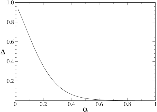
Figure 1: The error $\Delta$ of eq. (63) as a function of $\alpha$.

5 Driven system

Now, let us consider a system driven by an external Langevin heat-bath which has been considered by several authors [17, 18, 19, 20]. The velocities of the particles, evolve between collisions according to an Ornstein-Uhlenbeck process:

$$\frac{dv_{i}}{dt}=-\Gamma v_{i}(t)+\xi_{i}(t)$$ (64)

with

$$\langle\xi_{i}(t)\rangle=0,\qquad\langle\xi_{i}(t)\xi_{j}(t^{\prime})\rangle=2D\delta_{ij}\delta(t-t^{\prime})$$ (65)

The resulting equations for the distribution functions are:

$$\frac{d}{d\tau}\hat{f}_{1}(k_{1},\tau) = -(Dk_{1}^{2}+\Gamma k_{1}\frac{d}{dk_{1}})\hat{f}_{1}(k_{1},\tau)$$ (66)

$$+ \frac{1}{\tau_{c}}\{\hat{f}_{1}(\gamma k_{1},\tau)\hat{f}_{1}((1-\gamma)k_{1},\tau)-\hat{f}_{1}(k_{1},\tau)\hat{f}_{1}(0,\tau)$$

$$+ \frac{1}{N}[\hat{h}_{2}(\gamma k_{1},(1-\gamma)k_{1},\tau)-\hat{h}_{2}(k_{1},0,\tau)]\}$$

where an arbitrary mean free $\tau_{c}$ time has now been introduced for dimensional reasons, and

$$\frac{d}{d\tau}\hat{h}_{2}(k_{1},k_{2},\tau) = -[D(k_{1}^{2}+k_{2}^{2})+\Gamma(k_{1}\frac{d}{dk_{1}}+k_{2}\frac{d}{dk_{2}})]\hat{h}_{2}(k_{1},k_{2}\tau)$$

$$+ \frac{1}{\tau_{c}}\{\frac{1}{N}[\hat{h}_{2}(\gamma k_{1}+(1-\gamma)k_{2},\gamma k_{2}+(1-\gamma)k_{1},\tau)-\hat{h}_{2}(k_{1},k_{2},\tau)]$$

$$+ \hat{f}_{1}(\gamma k_{1}+(1-\gamma)k_{2},\tau)\hat{f}_{1}(\gamma k_{2}+(1-\gamma)k_{1},\tau)-\hat{f}_{1}(k_{1},\tau)\hat{f}_{1}(k_{2},\tau)$$

$$+ (1+P_{12})[\hat{f}_{1}((1-\gamma)k_{1},\tau)\hat{h}_{2}(\gamma k_{1},k_{2},\tau)-\hat{f}_{1}(0,\tau)\hat{h}_{2}(k_{1},k_{2},\tau)$$

$$+ \hat{f}_{1}(\gamma k_{1},\tau)\hat{h}_{2}(k_{2},(1-\gamma)k_{1},\tau)-\hat{f}_{1}(k_{1},\tau)\hat{h}_{2}(k_{2},0,\tau)]\}$$

We look for steady state solutions, setting the time derivatives to zero. By slightly modifying the method employed to derive the moments in the cooling case we obtain the moments in the non equilibrium steady state regime. We find:

$$M_{0} = 1$$ (68)

$$M_{2} = \frac{D\tau_{c}}{\Gamma\tau_{c}+\gamma(1-\gamma)}$$ (69)

$$M_{4} = \frac{12D\tau_{c}M_{2}+6\gamma^{2}(1-\gamma)^{2}M_{2}^{2}}{4\Gamma\tau_{c}+1-\gamma^{4}-(1-\gamma)^{4}}$$ (70)

$$= \frac{12[\Gamma\tau_{c}+\gamma(1-\gamma)]+6\gamma^{2}(1-\gamma)^{2}}{4\Gamma\tau_{c}+1-\gamma^{4}-(1-\gamma)^{4}}M_{2}^{2}$$

The granular temperature $T_{g}=mM_{2}$ is obtained from equation (69), yielding in the elastic case ($\gamma=0$) $T_{g}=mD/\Gamma$ as expected. Furthermore, the last equations in the elastic case becomes $M_{4}=3M_{2}^{2}$.

Similarly we find the coefficients of the moments of the pair correlation $h_{2}$ using in eq. (LABEL:bde2) the expansion (30)

$$Q_{n0} = Q_{0n}=-M_{n}$$ (71)

$$Q_{11} = \frac{\gamma(1-\gamma)}{\Gamma\tau_{c}}M_{2}$$ (72)

$$Q_{12} = Q_{21}=0$$ (73)

$$Q_{13} = Q_{31}=\frac{\gamma(1-\gamma)[1-2\gamma(1-\gamma)](3M_{2}^{2}+M_{4})+3\Gamma\tau_{c}Q_{11}^{2}+6D\tau_{c}Q_{11}}{4\Gamma\tau_{c}+3\gamma(1-\gamma)}$$ (74)

$$Q_{22} = \frac{\gamma^{2}(1-\gamma)^{2}(3M_{2}^{2}+M_{4})-2D\tau_{c}M_{2}}{2\Gamma\tau_{c}+2\gamma(1-\gamma)}$$ (75)

$$= \frac{\gamma^{2}(1-\gamma)^{2}(C+3)-2\Gamma\tau_{c}-2\gamma(1-\gamma)}{2\Gamma\tau_{c}+2\gamma(1-\gamma)}M_{2}^{2},$$

where in the last passage we have introduced the constant $C=M_{4}/M_{2}^{2}$. Again one can wonder the ratio between energy fluctuations and the square of granular temperature, obtaining:

$$\frac{\langle E^{2}(t)\rangle-\langle E(t)\rangle^{2}}{T_{g}(t)^{2}}=\frac{N}{2}\frac{2\Gamma\tau_{c}+\gamma(1-\gamma)[2+\gamma(\gamma+5)]}{2\Gamma\tau_{c}+\gamma(1-\gamma)[2-\gamma(1-\gamma)]}$$ (76)

which yields the value $N/2$ in the elastic case [21, 22].

Switching to the reduced variable $c^{2}=v^{2}/(2M_{2})$ we can look for an expression of the distribution function in terms of Sonine polynomials:

$$f_{1}(c)\simeq\frac{1}{\sqrt{\pi}}e^{-c^{2}}[1+s_{2}S_{2}(c^{2})+..]$$ (77)

with $s_{2}=-1+M_{4}/3M_{2}^{2}$ and $S_{2}(c^{2})=\frac{3}{8}-\frac{3}{2}c^{2}+\frac{1}{2}c^{4}$. In practice, one approximates the series (77) with a finite number of terms and since the leading term is the Maxwellian, the closer the system to the elastic limit, the less term suffice to describe the state. In the same spirit we assume the following expansion for the two-particle distribution function expression

$$h_{2}(c_{1},c_{2}) = -f_{1}(c_{1})f_{1}(c_{2})+\frac{1}{\pi}\exp{\left[-(c_{1}^{2}+c_{2}^{2})\right]}[A_{1}c_{1}c_{2}$$ (78)

$$+ A_{2}(\frac{1}{2}-c_{1}^{2})(\frac{1}{2}-c_{2}^{2})+A_{3}(c_{1}c_{2}^{3}+c_{1}^{3}c_{2})]$$

where the coefficients $A_{i}$ satisfy the relations:

$$A_{1} = \frac{8Q_{11}}{M_{2}}-\frac{2Q_{13}}{M_{2}^{2}}$$ (79)

$$A_{2} = 1+\frac{Q_{22}}{M_{2}^{2}}$$ (80)

$$A_{3} = -\frac{2Q_{11}}{M_{2}}+\frac{2Q_{13}}{3M_{2}^{2}}$$ (81)

A straightforward computation shows that $A_{i}\to 0$ (for $i=1,2,3$) in the elastic limit $\alpha\to 1$ and in the Brownian limit $\Gamma\tau_{c}\to\infty$, i.e. when the collision rate is so small that grains thermalize with the external bath.

6 Conclusion

We have shown that if the number, $N$, of particles, experiencing inelastic collisions described by the Inelastic Maxwell Model, is finite it is possible to observe correlations of order $1/N$ among the velocities of different particles. Such correlations have been studied in two relevant situations: the homogeneous cooling state and the steady state obtained by applying a stochastic driving to the system. In the first case we have obtained the velocity correlations by solving to order $1/N$ the equations for the moments of the one and two-particles distribution functions which show that the energy fluctuations decrease slower than the squared energy. In addition, we have studied the velocity pair correlation function in the scaling regime where the one-particle probability distribution is given by $f_{1}(u,t)=2[\pi v_{0}(t)]^{-1}[1+(u/v_{0}(t))^{2}]^{-2}$. For small inelasticity we have obtained its explicit expression. Interestingly, such a solution shows that the moment $Q_{22}$ of the velocity pair distribution function diverges. We may conjecture that such tails, which are the fingerprint of the Maxwell model, will persist in the many-particles correlation functions of higher order. These could be in principle computed using the same methods discussed above, although the effort required to carry out the program could be exceedingly heavy.

Finally, we have obtained, by the series expansion method, the pair distribution function when the system is subjected to a Langevin driving. In this case the moments of the pair correlation are finite up to the fourth order and we believe that the higher moments will also be finite.

As final remark we would like to comment that although the Maxwell model is somehow artificial and does not describe any real granular material it offers, as our paper illustrates, the possibilty of exploring new aspects of non equilibrium statistical systems. Acknowledgments.– U.M.B.M. acknowledges the support of the Project COFIN-MIUR 2005, 2005027808.

Appendix A Projection technique

Since we are not able to find a solution in the full space we resort to an approximate method in the remaining Fourier space. The method consists of projecting the term onto the subspace spanned by the function $\hat{\xi}_{n}$. For the sake of simplicity we define the scalar product between two functions $f$ and $g$

$$(f,g)=\int_{-\infty}^{+\infty}dqf(q)g(q)$$ (82)

and introduce an orthogonal basis, $R_{n}(q)$, of the form

$$R_{n}(q)=\sum_{l=1}^{n}A_{nl}|q|^{l}\exp(-|q|)$$ (83)

The orthonormalization conditions for $q_{1}q_{2}<0$ give the following relations:

$$R_{0}(|q|) = 2^{1/4}(\xi_{0}-\xi_{1}+\xi_{2})$$ (84)

$$R_{1}(|q|) = 2^{1/4}(\xi_{0}-3\xi_{1}+3\xi_{2})$$ (85)

$$R_{2}(|q|) = 2^{1/4}(\xi_{0}-5\xi_{1}+7\xi_{2})$$ (86)

in compact form:

$$R_{m}(|q|)=\sum_{n}M_{mn}\xi_{n}$$ (87)

We define, using the Heaviside function $\theta(x)$, $\tilde{U}(q_{1},q_{2})=[1-\theta(q_{1}q_{2})]U(q_{1},q_{2})$ and expand with respect to the $R_{n}$’s

$$\tilde{U}(q_{1},q_{2})=\sum_{a,b=0}^{2}U_{ab}R_{a}(q_{1})R_{b}(q_{2})+K(q_{1},q_{2})$$ (88)

where

$$U_{ab}=\int_{-\infty}^{+\infty}\int_{-\infty}^{+\infty}dq_{1}dq_{2}R_{a}(q_{1})R_{b}(q_{2})\tilde{U}(q_{1},q_{2})$$ (89)

and $K(q_{1},q_{2})$ represents the part of the function $\tilde{U}(q_{1},q_{2})$ orthogonal to the subspace spanned by the three functions above.

Inserting the ansatz $\chi_{2}(q_{1},q_{2})=\sum_{a,b}C_{ab}\xi_{a}(q_{1})\xi_{b}(q_{2})$ into (50), neglecting the term $K(q_{1},q_{2})$ and using (87) we obtain

$$[\Lambda_{1}+\Lambda_{2}]\sum_{a,b}C_{ab}\xi_{a}(q_{1})\xi_{b}(q_{2})=\sum_{m,n=0}^{2}T_{mn}\xi_{m}(q_{1})\xi_{n}(q_{2})$$ (90)

where $T_{mn}=\sum_{a,b=0}^{2}U_{ab}M_{am}M_{bn}$. Substituting the expansion of $T_{mn}$ up to third order in $\zeta$ we find the following equation for the coefficients $C_{mn}$:

$$\zeta \Big{[}C_{01}\xi_{0}(q_{1})\xi_{1}(q_{2})+C_{00}\xi_{0}(q_{1})\xi_{2}(q_{2})+C_{10}\xi_{1}(q_{1})\xi_{0}(q_{2})+2C_{11}\xi_{1}(q_{1})\xi_{1}(q_{2})$$ (91)

$$+ (C_{10}+C_{12})\xi_{1}(q_{1})\xi_{2}(q_{2})+C_{00}\xi_{2}(q_{1})\xi_{0}(q_{2})+[C_{01}+C_{21}]\xi_{2}(q_{1})\xi_{1}(q_{2})$$

$$+ [C_{02}+C_{20}]\xi_{2}(q_{1})\xi_{2}(q_{2})\Big{]}=7\zeta^{3}\xi_{0}(q_{1})\xi_{0}(q_{2})$$

$$- (\frac{3}{2}\zeta^{2}+33\zeta^{3})(\xi_{0}(q_{1})\xi_{1}(q_{2})+\xi_{1}(q_{1})\xi_{0}(q_{2}))+(-2\zeta+21\zeta^{2}+135\zeta^{3})\xi_{1}(q_{1})\xi_{1}(q_{2})$$

$$+ (-\zeta+\frac{3}{2}\zeta^{2}+45\zeta^{3})(\xi_{0}(q_{1})\xi_{2}(q_{2})+\xi_{2}(q_{1})\xi_{0}(q_{2}))$$

$$+ (\zeta-32\zeta^{2}-161\zeta^{3})(\xi_{2}(q_{1})\xi_{1}(q_{2})+\xi_{2}(q_{2})\xi_{1}(q_{1}))$$

$$+ (39\zeta^{2}+147\zeta^{3})\xi_{2}(q_{1})\xi_{2}(q_{2})$$

whose solution is given by eqs. (56)-(60)

Appendix B Small terms

In order to validate our assumption of neglecting the $1/N$ terms, we have evaluated the terms on the r.h.s. of eq. (23) using the relations given by eqs. (37)-(40). We obtain that the $1/N$ terms are null up to third order and the corresponding $k_{1}^{4}$ terms are explicitly

$$\hat{f}_{1}(\gamma k_{1},\tau)\hat{f}_{1}((1-\gamma)k_{1},\tau)-f_{1}(k_{1},\tau)$$

$$\approx...+\frac{1}{12}\Big{\{}\zeta^{2}\big{[}M_{4}(0)+3M_{2}^{2}(0)\big{]}e^{-a_{4}\tau}-2\zeta M_{4}(\tau)\Big{\}}k_{1}^{4}+...$$ (92)

$$\frac{1}{N}\Big{[}\hat{h}_{2}(\gamma k_{1},(1-\gamma)k_{1},\tau)-\hat{h}_{2}(k_{1},0,\tau)\Big{]}$$

$$\approx\frac{1}{4N}\Big{\{}\zeta^{2}\big{[}Q_{22}(0)-M_{4}(0)\big{]}e^{-2a_{2}\tau}+2\zeta^{2}M_{4}(\tau)\Big{\}}k_{1}^{4}+...$$ (93)

Comparing both coefficients we can state that our assumption is accurate at least up to fourth order.

References

• [1] Pöschel T and Luding S (eds.), Granular Gases, 2001 Lecture Notes in Physics, Vol. 564, Springer, Berlin
• [2] Brey J J, Dufty J W and Santos A, Dissipative dynamics for hard spheres, 1997 J. Stat. Phys 87 1051
• [3] van Noije T P C and Ernst M H, Velocity Distributions in Homogeneously Cooling and Heated Granular Fluids, 1998 Granular Matter 1 57
• [4] Baldassarri A, Marconi U M B, and Puglisi A, Influence of correlations on the velocity statistics of scalar granular gases, 2002 Europhys. Lett. 58 14 and Kinetic Models of Inelastic Gases, 2002 Math. Mod. Meth. Appl. Sci. 12 965
• [5] Marconi U M B and Puglisi A, Mean-field model of free-cooling inelastic mixtures, 2002 Phys. Rev. E 65 051305
• [6] Ben-Naim E and Krapivsky P L, Multiscaling in inelastic collisions, 2000 Phys. Rev. E 61 R5
• [7] Santos A, Transport coefficients of d-dimensional inelastic Maxwell models, 2002 Physica A 321 442
• [8] Ernst M H and Brito R, High-energy tails for inelastic Maxwell models, 2002 Eurohys. Lett. 58 182
• [9] Goldhirsch I and Zanetti G, Clustering instability in dissipative gases, 1993 Phys. Rev. Lett. 70 1619
• [10] Sela N and Goldhirsch I, Hydrodynamic equations for rapid flows of smooth inelastic spheres, to Burnett order, 1998 J. Fluid Mech. 361 41
• [11] Baldassarri A, Marconi U M B, and Puglisi A, Cooling of a lattice granular fluid as an ordering process, 2002 Phys. Rev. E 65 051301
• [12] van Noije T P C, Ernst M H, Brito R, Orza J A G, Mesoscopic Theory of Granular Fluids, 1997 Phys. Rev. Lett. 79 411
• [13] Brey J J, Moreno F and Ruiz-Montero M J, Spatial correlations in dilute granular flows: A kinetic model study, 1998 Phys.Fluids 10 2965
• [14] Soto R, Piasecki J and Mareschal M, Precollisional velocity correlations in a hard-disk fluid with dissipative collisions, 2001 Phys. Rev. E 64 031306
• [15] Brey J J, García de Soria M I, Maynar P and Ruiz-Montero M J, Energy fluctuations in the homogeneous cooling state of granular gases, 2004 Phys. Rev. E 70 011302
• [16] Bobylev A V, Exact solutions of the Boltzmann equation, 1976 Sov. Phys. Dokl. 20 820
• [17] Pagnani R, Marconi U M B and Puglisi A, Driven low density granular mixtures, 2002 Phys. Rev. E 66 051304
• [18] Marconi U M B and Puglisi A, Steady-state properties of a mean-field model of driven inelastic mixtures, 2002 Phys. Rev. E 66 011301
• [19] Ernst M H and Brito R, Driven inelastic Maxwell models with high energy tails, 2002 Phys. Rev. E 65 040301(R)
• [20] Santos A and Ernst M H, Exact steady-state solution of the Boltzmann equation: A driven one-dimensional inelastic Maxwell gas, 2003 Phys. Rev. E 68 011305
• [21] Cecconi F, Diotallevi F, Marconi U M B and Puglisi A, Fluid-like behavior of a one-dimensional granular gas, 2004 J. Chem. Phys 120 35
• [22] Visco P, Puglisi A, Barrat A, van Wijland F and Trizac E, Energy fluctuations in vibrated and driven granular gases, 2006 Eur. Phys. J B 51 377
• [23] Brey J J, Dufty J W, Ruiz-Montero M J, Linearized Boltzmann Equation and Hydrodynamics for Granular Gases, (2004) in Granular Gas Dynamics - Lecture Notes in Physics, Spinger (Berlin)