Quantum fluctuations in the transverse Ising spin glass model: A field theory of random quantum spin systems

Abstract

We develop a mean-field theory for random quantum spin systems using the spin coherent state path integral representation. After the model is reduced to the mean field one-body Hamiltonian, the integral is analyzed with the aid of several methods such as the semiclassical method and the gauge transformation. As an application we consider the Sherrington-Kirkpatrick model in a transverse field. Using the Landau expansion and its improved versions, we give a detailed analysis of the imaginary-time dependence of the order parameters. Integrating out the quantum part of the order parameters, we obtain the effective renormalized free energy written in terms of the classically defined order parameters. Our method allows us to obtain the spin glass-paramagnetic phase transition point $\Gamma/J\sim 1.62$ at $T=0$.

I Introduction

The classical random spin systems show various interesting properties that cannot be observed in clean systems. MPV ; Nishimori The main concern is the existence of the spin glass phase and comprehensive analyses of several models such as the Edwards-Anderson EA and the Sherrington-Kirkpatrick (SK) model SK have revealed the properties of the randomness-induced phase transition.

However, once we apply a transverse field to the SK model, the model becomes a quantum mechanical one and cannot be solved exactly even at the mean field level. CDS Since the work of Bray and Moore BM for the Heisenberg model, quantum spin glass models have attracted much interest as they can study the interplay between randomness and quantum fluctuations.

The effect of quantum fluctuations can be easily realized by formulating the models in a path integral form. It is well known that the $d$-dimensional quantum systems are mapped onto the $(d+1)$-dimensional classical systems. Sachdev In the mean-field analysis, models are described by the functional integral of order parameters and the additional coordinate (“time”) dependence demonstrates the fluctuation effects. The simplest possible approximation is to neglect the time dependence of order parameters, which misses quantum effects and is not generally justified.

Concerning the SK model in a transverse field, the spin glass phase transition has been investigated by many authors. IY ; U ; YI ; WL ; Y ; TLK ; GL ; UBK ; MH ; RGAR ; KK It was recognized there that the static approximation is not justified at low temperature and the spin-glass–paramagnetic-phase transition point at $T=0$ is significantly affected by quantum effects.

In this paper, we propose a systematic method for quantum random spin systems. It is based on expressing the partition function using a path integral form. Using the Trotter-Suzuki decomposition TS we insert the spin coherent state representation as the resolution of unity. The use of coherent states has great advantage for the resulting integrals since the spin integral variables are continuous. Furthermore this method can be applied to the arbitrary Hamiltonian. The use of the spin coherent states is inevitable for the quantum Heisenberg model and was indeed done in Ref.SYGPS, . Although it is not necessary for the SK model, we stress in this paper that our method is convenient for the systematic calculations. We mention, for example, the semiclassical method and the gauge transformation.

We apply our formulation to the transverse SK model. We carefully treat the time dependence of the order parameters to investigate the spin-glass–paramagnetic-phase transition. We use several field theoretical methods: the Landau expansion, the renormalization-group-like method at finite temperature, and the derivative expansion at zero temperature. The result of the phase diagram is compared to the previous works.

The paper is organized as follows. In Sec.II we introduce a path integral form for the general quantum spin Hamiltonian and discuss several methods to calculate the functional integral. In Sec.III we apply the method to the transverse SK model. After discussing the Landau expansion, we consider improved methods to treat the quantum fluctuations. We calculate the spin glass order parameter and determines the phase diagram. Section IV is devoted to discussions and conclusions.

II Formulation for quantum spin systems

II.1 Coherent state path integral representation

The path integral representation for spin systems can be found in, e.g., Refs.K, ; cs, ; WFS, ; AG, . The closure relation is expressed by using the spin coherent states and is inserted to the Trotter-Suzuki decomposition TS of the matrix element of the time evolution operator. The spin operators in the Hamiltonian are replaced by the classical variables, and the complex phase factor is added to ensure the dynamics.

The spin coherent state for spin $S$ is defined by

$$|{\bf S}\rangle=e^{-i\varphi\hat{S}_{3}}e^{-i\theta\hat{S}_{2}}|S\rangle,$$ (1)

where $\hat{{\bf S}}=(\hat{S}_{1},\hat{S}_{2},\hat{S}_{3})$ are spin operators satisfying

$$[\hat{S}_{i},\hat{S}_{j}]=i\epsilon_{ijk}\hat{S}_{k},\quad\hat{{\bf S}}^{2}=S(S+1),$$ (2)

and $|S\rangle$ denotes the eigenstate of $\hat{S}_{3}$ with the eigenvalue $S$. $\theta$ and $\varphi$ are real parameters and parametrize the coordinates on a unit sphere. The expectation value of the spin operators is given by

$${\bf S}=\langle{\bf S}|\hat{{\bf S}}|{\bf S}\rangle=S(\sin\theta\cos\varphi,\sin\theta\sin\varphi,\cos\theta).$$ (3)

The closure relation is written as

$$\int d{\bf S}|{\bf S}\rangle\langle{\bf S}|=\frac{2S+1}{4\pi}\int_{-1}^{1}d(\cos\theta)\int_{0}^{2\pi}d\varphi|{\bf S}\rangle\langle{\bf S}|=1.$$ (4)

We consider the finite temperature partition function for the quantum spin Hamiltonian $\hat{H}=H[\hat{{\bf S}}]$. We use the Trotter decomposition and insert the coherent states defined above. We have the matrix element

$$\langle{\bf S}(\tau+\Delta\tau)|e^{-\Delta\tau\hat{H}}|{\bf S}(\tau)\rangle\sim\exp\left\{\Delta\tau\left[-\langle{\bf S}(\tau)|\frac{d}{d\tau}|{\bf S}(\tau)\rangle-\langle{\bf S}(\tau)|\hat{H}|{\bf S}(\tau)\rangle\right]\right\},$$ (5)

where $\tau$ is the slice index and represents the imaginary time between 0 and $\beta=1/k_{B}T$, and $\Delta\tau$ is the slice width which must be taken $\Delta\tau\to 0$. The first term on the right-hand side is pure imaginary and includes the time derivative. The second term gives the Hamiltonian with the operators replaced by the classical variables given by Eq.(3). Thus, we arrive at the expression for the finite temperature partition function

$$Z=\int{\cal D}{\bf S}\exp\left\{i\int_{0}^{\beta}d\tau\Phi(\tau)-\int_{0}^{\beta}d\tau H[{\bf S}(\tau)]\right\},$$ (6)

where

$$\Phi(\tau)=i\langle{\bf S}(\tau)|\frac{d}{d\tau}|{\bf S}(\tau)\rangle=S\dot{\varphi}(\tau)\cos\theta(\tau),$$ (7)

and the periodic boundary condition ${\bf S}(0)={\bf S}(\beta)$ is imposed. We note that $\Phi$ represents the geometric Berry phase. The corresponding term in Eq.(6) is always imaginary irrespective of the real or imaginary time formulations and describes the dynamical motion of ${\bf S}(\tau)$ on the sphere.

II.2 Calculation methods

As we mentioned above, the advantage of the coherent state representation is that the spin operators are replaced by the continuous classical variables, which is crucial to describe the spin dynamics. Various methods developed in the path integral formalism can be applied to the present case as well. Here we discuss two useful methods used in the following sections. Without loss of generality in the present context we can confine our discussion to the one-body Hamiltonian

$$\hat{H}=-{\bf B}\cdot\hat{{\bf S}},$$ (8)

where $B$ is the external magnetic field which may depend on time. In the following application of a spin glass model, the system can be written in the one-body form by introducing the auxiliary variables.

II.2.1 Semiclassical method

First, we mention the semiclassical method which is known as the standard approximation in the path integral formalism. We assume the main contribution comes from the stationary configuration of spin variables. The assumption is justified when $\hbar=0$ and hence the name semiclassical. The stationary phase equation is nothing but the classical equation of motion

$$i\frac{d{\bf S}(\tau)}{d\tau}={\bf S}(\tau)\times\frac{\partial H}{\partial{\bf S}(\tau)}.$$ (9)

For the Hamiltonian (8), it is known that this approximation becomes exact in the coherent state representation. The derived path integral representation is ill-defined and we need a regularization to perform the integral explicitly. Klauder K used the Wiener regularization and considered the path integral using the stationary phase (saddle point) approximation. It was proved, after 20 years, that the approximation becomes exact for the one-body Hamiltonian. AG The problem is reduced to solving the classical equation of motion (9) under the arbitrary boundary condition. The reason why the stationary phase approximation becomes exact is that the coherent states satisfy the minimal uncertainty relation.

In the following application discussed in the next section, this method turns out to be useful when we calculate the correlation function. For example, we consider the spin-$1/2$ system with the Hamiltonian $\hat{H}=-2\Gamma\hat{S}_{3}$. The correlation function in the perpendicular (say, $y$) direction to the magnetic field $\Gamma$ can be written as

$$D(\tau-\tau^{\prime})=\frac{\int{\cal D}{\bf S}n_{y}(\tau)n_{y}(\tau^{\prime})\exp\left[i\int_{\tau}\Phi(\tau)+\int_{\tau}\Gamma n_{z}(\tau)\right]}{\int{\cal D}{\bf S}\exp\left[i\int_{\tau}\Phi(\tau)+\int_{\tau}\Gamma n_{z}(\tau)\right]},$$ (10)

where ${\bf S}=S{\bf n}={\bf n}/2$ and $\int_{\tau}=\int_{0}^{\beta}d\tau$. The result of the integration is given by

$$D(\tau-\tau^{\prime})=\frac{e^{\beta\Gamma-2\Gamma|\tau-\tau^{\prime}|}+e^{-\beta\Gamma+2\Gamma|\tau-\tau^{\prime}|}}{e^{\beta\Gamma}+e^{-\beta\Gamma}}.$$ (11)

This form is known and can be obtained by using other methods such as the transfer matrix method. Competitive advantage of the present method arises when we generalize the calculation to higher order correlation functions and higher spins with $S>1/2$.

II.2.2 Gauge transformation

Second, the gauge transformation is utilized when we calculate the correlation functions. The basis of the state to be inserted into the Trotter decomposition can be changed to other arbitrary basis. We consider the rotation in spin space by the unitary operator

$$\hat{U}[\mbox{{\boldmath$\phi$}}(\tau)]=\exp\left[i\int_{\tau}\mbox{{\boldmath$\phi$}}(\tau)\cdot\hat{\bf S}\right].$$ (12)

The partition function of the Hamiltonian (8) can be written as

$$Z=\int{\cal D}{\bf S}\exp\left[i\int_{\tau}\Phi(\tau)+\int_{\tau}{\bf B}(\tau)\cdot{\bf S}(\tau)\right].$$ (13)

We consider the time-dependent rotation diagonalizing the Hamiltonian to $\hat{H}=-|{\bf B}(\tau)|\hat{S}_{3}$. Such a choice is always possible, but this does not solve the problem because we have the expression

$$Z=\int{\cal D}{\bf S}\exp\left\{i\int_{\tau}\left[\Phi(\tau)+\dot{\mbox{{\boldmath$\phi$}}}(\tau)\cdot{\bf S}(\tau)\right]+\int_{\tau}|{\bf B}(\tau)|S_{3}(\tau)\right\}.$$ (14)

Due to the time-dependent gauge transformation, the phase acquires an extra term. This cannot be solved generally except simple cases such as constant fields and oscillating fields. This type of the gauge transformation was discussed in Ref.SF, and the extra term of Eq.(14) is called the geometric phase. This expression can be utilized when we consider the derivative expansion. When the time-dependence is slow, the geometric phase term is expanded and the only remaining thing to do is to calculate the correlation functions as Eq.(10).

III Application to the Sherrington-Kirkpatrick model in a transverse field

As an application of the spin coherent path integral representation we consider the transverse SK model defined by the Hamiltonian with Pauli spins $\hat{\bf S}=\mbox{\boldmath$\sigma$}/2$ on lattice sites

$$\hat{H}=-\frac{1}{2}\sum_{i\neq j}^{N}J_{ij}\sigma^{z}_{i}\sigma^{z}_{j}-\Gamma\sum_{i=1}^{N}\sigma_{i}^{x},$$ (15)

where $J_{ij}$ is the Gaussian random variables with mean $J_{0}/N$ and variance $J^{2}/N$, $N$ is the number of lattice sites, and $\Gamma$ is the transverse field. $i$ and $j$ run over all points, which means that the interaction is infinite range and the mean-field analysis becomes exact. When the transverse field is present, the model cannot be solved exactly and we need an approximation. As we explained in the Introduction, the simplest way to proceed is to neglect the time dependence of the order parameters introduced as auxiliary integral variables. It looks plausible because the time variable is introduced artificially and its dependence cannot directly be observed. However, we discuss in the following that the time dependence should be integrated out rather than be neglected, which gives a nontrivial quantum effect.

III.1 Mean field theory

We follow the standard prescription to introduce the auxiliary fields $m$ and $q$ using the Hubbard-Stratonovich transformation. MPV ; Nishimori Introducing replicas, we take the average of the $n$th power of the partition function as

$$[Z^{n}] = \int{\cal D}{\bf S}\exp\biggl{\{}\sum_{a=1}^{n}\sum_{i=1}^{N}\int_{\tau}\left[i\Phi_{i}^{a}(\tau)+\Gamma n_{xi}^{a}(\tau)\right]$$ (16)

$$+\frac{J_{0}}{N}\sum_{a=1}^{n}\sum_{i<j}^{N}\int_{\tau}n^{a}_{zi}(\tau)n^{a}_{zj}(\tau)+\frac{J^{2}}{2N}\sum_{a,b=1}^{n}\sum_{i<j}^{N}\int_{\tau,\tau^{\prime}}n^{a}_{zi}(\tau)n^{a}_{zj}(\tau)n^{b}_{zi}(\tau^{\prime})n^{b}_{zj}(\tau^{\prime})\biggr{\}}.$$

The Hubbard-Stratonovich transformation allows us to introduce the order parameters. We have

$$[Z^{n}]=\int{\cal D}m{\cal D}q\exp\biggl{\{}-\frac{NJ_{0}}{2}\sum_{a=1}^{n}\int_{\tau}\left[m_{a}(\tau)\right]^{2}-\frac{NJ^{2}}{4}\sum_{a,b=1}^{n}\int_{\tau,\tau^{\prime}}\left[q_{ab}(\tau,\tau^{\prime})\right]^{2}+N\ln\mbox{Tr}\,e^{L}\biggr{\}},$$ (17)

where

$$\mbox{Tr}\,e^{L} = \int{\cal D}{\bf S}\exp\biggl{\{}\sum_{a=1}^{n}\int_{\tau}\left[i\Phi^{a}(\tau)+\Gamma n_{x}^{a}(\tau)+J_{0}m_{a}(\tau)n^{a}_{z}(\tau)\right]+\frac{J^{2}}{2}\sum_{a,b=1}^{n}\int_{\tau,\tau^{\prime}}q_{ab}(\tau,\tau^{\prime})n^{a}_{z}(\tau)n^{b}_{z}(\tau^{\prime})\biggr{\}}.$$ (18)

The saddle point equations

$$m_{a}(\tau)=\frac{\mbox{Tr}\,n_{z}^{a}(\tau)e^{L}}{\mbox{Tr}\,e^{L}},\quad q_{ab}(\tau,\tau^{\prime})=\frac{\mbox{Tr}\,n_{z}^{a}(\tau)n_{z}^{b}(\tau^{\prime})e^{L}}{\mbox{Tr}\,e^{L}}$$ (19)

indicate that $m$ is the magnetization and $q$ the spin glass order parameter.

III.2 Landau expansion

To proceed further, we must integrate out the spin variables ${\bf n}^{a}(\tau)$ to get the order parameter functional. We do this by using the Landau expansion assuming the order parameters are small. The Landau theory for the present model was considered in Ref.RSY, by writing down the functional immediately from the symmetry argument. That method is phenomenological and the coupling constants in the Landau function cannot be related to the fundamental parameters in the original Hamiltonian. Here we derive the Landau function microscopically from the original Hamiltonian. We use the derived result to determine the phase boundary where the approximation makes sense. Then the transition point can be expressed by $T/J$ and $\Gamma/J$.

In order to get the result we must calculate the spin correlation function (11). Higher order correlation functions can be calculated in the same way as the two point function. For instance the four point function is

$$D(\tau_{1},\tau_{2},\tau_{3},\tau_{4})=D(\tau_{1}^{\prime}-\tau_{2}^{\prime}+\tau_{3}^{\prime}-\tau_{4}^{\prime}),$$ (20)

where $\tau_{1,2,3,4}$ are arranged in order of magnitude as $\tau_{1}^{\prime}>\tau_{2}^{\prime}>\tau_{3}>\tau_{4}^{\prime}$. Higher order functions can be expressed in the same way.

Now we can express each term of the Landau expansion using the correlation functions. For simplicity we consider $J_{0}m_{a}(\tau)=0$ which means we consider the paramagnetic or spin glass phase. We write for the spin glass order parameter

$$q_{ab}(\tau,\tau^{\prime})=\delta_{ab}\chi_{a}(\tau,\tau^{\prime})+(1-\delta_{ab})q_{ab}(\tau,\tau^{\prime}),$$ (21)

to distinguish the role of each term. The first term is the diagonal part in the replica space and represents the spin susceptibility. It is unity when $\Gamma=0$ and the deviation from unity at $\Gamma\neq 0$ represents the quantum effect. The second term is the familiar spin glass order parameter.

Using this representation, we can Landau-expand the averaged free energy as

$$\beta[f]=-\ln(e^{\beta\Gamma}+e^{-\beta\Gamma})+\lim_{n\to 0}\frac{1}{n}\left\{\frac{J^{2}}{4}\sum_{a=1}^{n}\int_{\tau}\chi_{a}^{2}(\tau)+\frac{J^{2}}{4}\sum_{a\neq b=1}^{n}\int_{\tau\tau^{\prime}}q_{ab}^{2}(\tau,\tau^{\prime})-\sum_{k=1}^{\infty}\frac{1}{k!}\left(\frac{J^{2}}{2}\right)^{k}I_{k}\right\},$$ (22)

where $I_{k}$ is of $k$th order in $\chi$ and $q$. For $k=1$ and 2, it is given by

$$I_{1}=\sum_{a=1}^{n}\int_{\tau_{1}\tau_{2}}\chi_{a}(\tau_{1},\tau_{2})D(\tau_{1}-\tau_{2}),$$ (23)

$$I_{2}=\sum_{a=1}^{n}\int_{\tau_{1}\tau_{2}\tau_{3}\tau_{4}}\chi_{a}(\tau_{1},\tau_{2})\chi_{a}(\tau_{3},\tau_{4})\left[D(\tau_{1},\tau_{2},\tau_{3},\tau_{4})-D(\tau_{1}-\tau_{2})D(\tau_{3}-\tau_{4})\right]$$

$$+2\sum_{a\neq b}^{n}\int_{\tau_{1}\tau_{2}\tau_{3}\tau_{4}}q_{ab}(\tau_{1},\tau_{3})q_{ba}(\tau_{4},\tau_{2})D(\tau_{1}-\tau_{2})D(\tau_{3}-\tau_{4}).$$ (24)

We note that this is the expansion in terms of $\beta^{2}J^{2}q_{ab}(\tau,\tau^{\prime})$ and $\beta^{2}J^{2}\chi_{a}(\tau,\tau^{\prime})$. Since the order parameters are unity at most, we can regard $\beta^{2}J^{2}$ as a formal expansion parameter. The order parameters are determined by the saddle point equations. In the following we consider the replica symmetric and nonsymmetric cases.

III.2.1 Replica symmetric solution

We assume that $\chi$ and $q$ are independent of the replica index. Then the saddle point equations up to first order in $\beta^{2}J^{2}$ are given by

$$\chi(\tau_{1},\tau_{2})=D(\tau_{1}-\tau_{2})+\frac{J^{2}}{2}\int_{\tau_{3}\tau_{4}}\chi(\tau_{3},\tau_{4})\left[D(\tau_{1},\tau_{2},\tau_{3},\tau_{4})-D(\tau_{1}-\tau_{2})D(\tau_{3}-\tau_{4})\right],$$ (25)

$$q(\tau_{1},\tau_{2})=J^{2}\int_{\tau_{3}\tau_{4}}q(\tau_{3},\tau_{4})D(\tau_{1}-\tau_{3})D(\tau_{4}-\tau_{2}).$$ (26)

At the linear approximation $\chi(\tau,\tau^{\prime})$ is equal to the correlation function $D(\tau-\tau^{\prime})$ and the assumption of the replica independence is plausible in the perturbative calculation. On the other hand, the time dependence of $\chi$ cannot be neglected. Concerning $q$, the static approximation seems to be appropriate as we discuss below.

$\chi$ can be solved iteratively while $q$ is solved by considering higher order nonlinear terms. The phase boundary can be determined by the leading term in Eq.(26). Using the static approximation for $q$, we obtain

$$1=J^{2}\left(\int_{\tau}D(\tau)\right)^{2}=\beta^{2}J^{2}\left(\frac{\tanh\beta\Gamma}{\beta\Gamma}\right)^{2}.$$ (27)

This can be easily solved to find $\Gamma/J=1$ at $T=0$. WL This perturbative solution is compared to the static approximation result $\Gamma/J=2$ in Refs.U, and TLK, where $\chi$ is not expanded and treated nonperturbatively. The difference comes from the fact that $\chi$ does not vanish at the phase boundary and contributes to Eq.(27).

III.2.2 Replica symmetry breaking solution

It is well known in the classical SK model without transverse field that the spin glass order parameter depends on the replica index and the replica symmetry breaking (RSB) solution proposed by Parisi Parisi is the exact one. Here we consider the effect of the transverse field for the RSB solution. The calculation can be done explicitly if we use the Landau expansion. The free energy is expanded in $q_{ab}$ up to the fourth order and the saddle-point equation is solved analytically under the assumption of the RSB. Parisi ; Nishimori This can be done even if the transverse field is incorporated. Near the transition point $T=T_{c}$, we obtain the expression

$$\beta[f] = \lim_{n\to 0}\frac{1}{n}\biggl{\{}\frac{1}{2}\theta\sum_{a\neq b}(Q_{ab})^{2}-\frac{1}{6}C_{1}\sum_{a\neq b\neq c}Q_{ab}Q_{bc}Q_{ca}-\frac{1}{12}C_{2}\sum_{a\neq b}(Q_{ab})^{4}$$ (28)

$$+\frac{1}{4}C_{3}\sum_{abc}(Q_{ab})^{2}(Q_{ac})^{2}-\frac{1}{8}C_{4}\mbox{Tr}\,(Q)^{4}\biggr{\}},$$

where $Q_{ab}=\beta^{2}J^{2}q_{ab}$ and $\theta=(T_{c}-T)/T_{c}$. $T_{c}$ and the coefficients $C_{1,2,3,4}$ depend on $\chi$ and are expressed perturbatively. We have for $C_{1,2}$

$$C_{1}=\left(\frac{1}{\beta}\int_{\tau}D(\tau)\right)^{3}+\frac{3}{2}\beta^{2}J^{2}\left(\frac{1}{\beta}\int_{\tau}D(\tau)\right)^{2}\frac{1}{\beta^{4}}\int_{\tau_{1-4}}\chi(\tau_{1},\tau_{2})\left[D(\tau_{1},\tau_{2},\tau_{3},\tau_{4})-D(\tau_{1}-\tau_{2})D(\tau_{3}-\tau_{4})\right]+\cdots,$$

$$C_{2}=-\frac{1}{2\beta^{8}}\int_{\tau_{1-8}}\left[D(\tau_{1},\tau_{2},\tau_{3},\tau_{4})D(\tau_{5},\tau_{6},\tau_{7},\tau_{8})-3D(\tau_{1}-\tau_{2})D(\tau_{3}-\tau_{4})D(\tau_{5}-\tau_{6})D(\tau_{7}-\tau_{8})\right]+\cdots.$$ (29)

$T_{c}$ and $C_{3,4}$ are expressed in a similar way. When $\Gamma=0$, all the correlation functions are set to unity and we obtain the classical result $C_{1,2,3,4}=1$. Since the effect of the transverse field is only to change the coefficients of the expansion (28), the saddle point equation for $Q_{ab}$ is easily solved in the same way as the classical case as

$$q(x)=\frac{C_{1}}{C_{2}}\frac{x}{2}\quad(0\leq x<x_{1}=2|\theta|C_{2}/C_{1}),$$

$$q(x)=|\theta|\quad(x_{1}\leq x\leq 1),$$ (30)

where $x$ is the replica continuous variable at $n\to 0$. Thus, the transverse field changes the slope of the line. Each term of the coefficient $C_{1,2}$ can be calculated analytically. If we keep only the leading term in Eq.(29) we have

$$\frac{C_{1}}{C_{2}}\sim\left(\frac{\tanh\beta\Gamma}{\beta\Gamma}\right)^{3}\frac{1}{\frac{3}{2}\left(\frac{\tanh\beta\Gamma}{\beta\Gamma}\right)^{4}-\frac{9}{2(\beta\Gamma)^{4}}\left(1-\frac{\tanh\beta\Gamma}{\beta\Gamma}\right)^{2}}.$$ (31)

This is larger than unity when $\beta\Gamma>0$, which means that the RSB solution approaches the replica symmetric solution and we expect that the stability of the replica symmetric solution increases. In the following calculations, we consider the replica symmetric solution and our attention is mainly focused on the time dependence of $\chi$.

III.3 Improved Landau expansion at classical regime

As we mentioned above the naive perturbative expansion gives the transition point $\Gamma=J$ at $T=0$ (Ref.WL, ) and the static approximation for $\chi$ gives $\Gamma=2J$ at $T=0$. U ; TLK Furthermore, several analyses using more sophisticated techniques showed that the transition point lies between them. YI ; MH In the following analysis, we reconsider this problem using a refined field theoretical method systematically. Our method allows us to obtain the phase structure not only at the boundary as was done in previous works but also in the whole space.

Equation (25) tells us that the order parameter $\chi(\tau_{1},\tau_{2})$ is approximately equal to the correlation function $D(\tau_{1}-\tau_{2})$ in Eq.(11). This function has a slow time dependence at $\beta\Gamma\ll 1$ and fast at $\beta\Gamma\gg 1$. Therefore, when the temperature is not so low, the static approximation is expected to be valid. On the other hand, it is not justified at low temperature.

First we treat the classical regime where the time dependence is not so strong. In this case we can separate the time-dependent and -independent parts of $\chi_{a}(\tau)$ and $q_{ab}(\tau,\tau^{\prime})$ as

$$\chi_{a}(\tau)=\chi+\tilde{\chi}_{a}(\tau),\quad q_{ab}(\tau,\tau^{\prime})=q+\tilde{q}_{ab}(\tau,\tau^{\prime}),$$ (32)

where $\chi$ and $q$ are zero modes defined as the zero frequency part of the Fourier transformation. $\tilde{\chi}_{a}(\tau)$ and $\tilde{q}_{ab}(\tau,\tau^{\prime})$ are expected to be small and we consider the Landau expansion in terms of these variables. On the other hand $\chi$ and $q$ are not expanded and treated nonperturbatively as was done in the static calculation. We expand the averaged free energy in terms of the nonstatic modes and integrate those modes as

$$[Z^{n}]=\int{\cal D}q{\cal D}\chi{\cal D}\tilde{q}{\cal D}\tilde{\chi}\exp\left\{-Nn\beta f[q,\chi,\tilde{q},\tilde{\chi}]\right\}=\int{\cal D}q{\cal D}\chi\exp\left\{-Nn\beta f_{\rm eff}[q,\chi]\right\}.$$ (33)

$f_{\rm eff}$ is defined as the classical free energy renormalized by the quantum part of the order parameters. $f$ is expanded in $\tilde{\chi}$ and $\tilde{q}$ up to second order and we carry out the Gaussian integrals. Thus the static and nonstatic parts are treated separately and we can take full advantage of both the Landau expansion and the static approximation.

Using the separation of order parameters, we have

$$\mbox{Tr}\,e^{L} = \int{\cal D}{\bf S}Dz\prod_{a}Dz_{a}\exp\biggl{[}\sum_{a}\int_{\tau}\left[i\Phi^{a}(\tau)+\Gamma n_{x}^{a}(\tau)+J(\sqrt{q}z+\sqrt{\chi-q}z_{a})n_{z}^{a}(\tau)\right]$$ (34)

$$\qquad\qquad+\frac{J^{2}}{2}\sum_{a}\int_{\tau\tau^{\prime}}\tilde{\chi}_{a}(\tau,\tau^{\prime})n^{a}_{z}(\tau)n^{a}_{z}(\tau^{\prime})+\frac{J^{2}}{2}\sum_{a\neq b}\int_{\tau\tau^{\prime}}\tilde{q}_{ab}(\tau,\tau^{\prime})n^{a}_{z}(\tau)n^{b}_{z}(\tau^{\prime})\biggr{]},$$

where we introduced the auxiliary variables $z$ and $z_{a}$ ($a=1,2,\ldots,n$), and the integration measures are given by

$$Dz=\frac{dz}{\sqrt{2\pi}}e^{-z^{2}/2},\quad Dz_{a}=\frac{dz_{a}}{\sqrt{2\pi}}e^{-z_{a}^{2}/2}.$$ (35)

The last two terms are expanded up to second order as

$$\mbox{Tr}\,e^{L} = \int Dz\prod_{a=1}^{n}Dz_{a}\prod_{a=1}^{n}(e^{\beta h_{a}}+e^{-\beta h_{a}})\exp\biggl{[}\frac{J^{2}}{2}\sum_{a=1}^{n}\frac{\Gamma^{2}}{h_{a}^{2}}\int d\tau d\tau^{\prime}\tilde{\chi}_{a}(\tau,\tau^{\prime})D_{h_{a}}(\tau-\tau^{\prime})$$ (36)

$$+\frac{J^{4}}{8}\sum_{a}\int_{\tau_{1,2,3,4}}\tilde{\chi}_{a}(\tau_{1},\tau_{2})\tilde{\chi}_{a}(\tau_{3},\tau_{4})\left[D_{h_{a}}(\tau_{1},\tau_{2},\tau_{3},\tau_{4})-D_{h_{a}}(\tau_{1},\tau_{2})D_{h_{a}}(\tau_{3},\tau_{4})\right]$$

$$+\frac{J^{4}}{4}\sum_{a\neq b}\int_{\tau_{1,2,3,4}}\tilde{q}_{ab}(\tau_{1},\tau_{2})\tilde{q}_{ab}(\tau_{3},\tau_{4})D_{h_{a}}(\tau_{1},\tau_{3})D_{h_{b}}(\tau_{2},\tau_{4})\frac{\Gamma^{2}}{h_{a}^{2}}\frac{\Gamma^{2}}{h_{b}^{2}}\biggr{]},$$

where

$$h_{a}=\sqrt{\Gamma^{2}+J^{2}(\sqrt{q}z+\sqrt{\chi-q}z_{a})^{2}},$$ (37)

and $D_{h_{a}}(\tau,\tau^{\prime})$ is the correlation function (11) with $\Gamma$ replaced by $h_{a}$. We used the gauge transformation to “diagonalize” the Hamiltonian. In the present case, the magnetic field is independent of time and the extra phase factor does not arise here. Then taking the $n\to 0$ limit we obtain

$$\lim_{n\to 0}\ln\mbox{Tr}\,e^{L} = \int Dz_{1}\ln\left[\int Dz_{2}(e^{\beta h}+e^{-\beta h})\right]$$

$$+\lim_{n\to 0}\frac{1}{n}\biggl{[}\frac{J^{2}}{2}\sum_{a=1}^{n}\int_{\tau\tau^{\prime}}\tilde{\chi}_{a}(\tau,\tau^{\prime})\int Dz_{1}D^{\prime}z_{2}D_{h}(\tau-\tau^{\prime})\frac{\Gamma^{2}}{h^{2}}$$

$$+\frac{J^{4}}{8}\sum_{a}\int_{\tau_{1,2,3,4}}\tilde{\chi}_{a}(\tau_{1},\tau_{2})\tilde{\chi}_{a}(\tau_{3},\tau_{4})\int Dz_{1}D^{\prime}z_{2}\left[D_{h}(\tau_{1},\tau_{2},\tau_{3},\tau_{4})-D_{h}(\tau_{1}-\tau_{2})D_{h}(\tau_{3}-\tau_{4})\right]$$

$$+\frac{J^{4}}{4}\sum_{a\neq b}\int_{\tau_{1,2,3,4}}\tilde{q}_{ab}(\tau_{1},\tau_{2})\tilde{q}_{ab}(\tau_{3},\tau_{4})\int Dz_{1}\left(\int D^{\prime}z_{2}D_{h}(\tau_{1}-\tau_{3})\frac{\Gamma^{2}}{h^{2}}\right)\left(\int D^{\prime}z_{2}D_{h}(\tau_{2}-\tau_{4})\frac{\Gamma^{2}}{h^{2}}\right)\biggr{]},$$

where $h$ is equal to $h_{a}$ with $z$ ($z_{a}$) replaced by $z_{1}$ ($z_{2}$), and

$$Dz_{1,2}=\frac{dz_{1,2}}{\sqrt{2\pi}}e^{-z_{1,2}^{2}/2},\qquad\int D^{\prime}z_{2}\left(\cdots\right)=\frac{\int Dz_{2}\left(\cdots\right)\cosh\beta h}{\int Dz_{2}\cosh\beta h}.$$ (39)

The integrations of the nonzero modes $\tilde{\chi}_{a}(\tau)$ and $\tilde{q}_{ab}(\tau)$ are easily carried out to obtain the renormalized effective free energy with the leading nontrivial contribution

$$\beta f_{\rm eff}\sim\frac{\beta^{2}J^{2}}{4}(\chi^{2}-q^{2})-\int Dz_{1}\ln\left[\int Dz_{2}(e^{\beta h}+e^{-\beta h})\right]-\frac{\beta^{2}J^{2}}{2}\sum_{m=1}^{\infty}\left(\int Dz_{1}D^{\prime}z_{2}\tilde{D}_{h}(m)\frac{\Gamma^{2}}{h^{2}}\right)^{2},$$ (40)

where $\tilde{D}_{h}(m)$ is the Fourier transformation of $D_{h}(\tau)$ and is given by

$$\tilde{D}_{h}(m)=\frac{(\beta h)^{2}}{(\beta h)^{2}+(\pi m)^{2}}\frac{\tanh\beta h}{\beta h}.$$ (41)

Up to the second order expansion of the nonzero modes, $\tilde{q}$ fluctuations do not contribute to the result. This is because the spin glass order parameter is defined as the global variable in terms of the lattice site index as $F=Nf[q]$. A different conclusion is obtained if we define $q$ as local order parameters $q_{i}$ and write $F[q]=\sum_{i}f[q_{i}]$. Fluctuations in each local site give a nontrivial result. Our model was defined as the infinite range model. In that case, $\tilde{q}$ fluctuations are not important and the static approximation for $\tilde{q}$ is justified. In this sense the mean field theory of the infinite range model is different from that of the finite range model as discussed in Ref.RSY, .

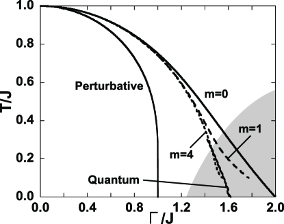
Figure 1: Phase boundary from the saddle point equations (42). The maximum frequency value of the summation is denoted with lines. “$m=0$” corresponds to the static approximation result and “Perturbative” denotes the naive Landau expansion result (27). “Quantum” is the result in Sec.III.4. The quantum regime is shown by the shaded area.

The effective free energy (40) is a function of $q$ and $\chi$. Their values are obtained by solving the saddle point equations $\partial f_{\rm eff}/\partial\chi=0$ and $\partial f_{\rm eff}/\partial q=0$. The phase boundary is determined by $\partial f_{\rm eff}/\partial\chi|_{q=0}=0$ and $\partial^{2}f_{\rm eff}/\partial^{2}q|_{q=0}=0$. Using formulas derived in the Appendix, we obtain

$$\chi=\frac{1}{\beta^{2}J^{2}\chi}\left(\int D^{\prime}zz^{2}-1\right)+\frac{1}{\chi}\sum_{m=1}^{\infty}\left(\int D^{\prime}z\tilde{D}_{h}(m)\frac{\Gamma^{2}}{h^{2}}\right)\left[\int D^{\prime}z\left(z^{2}-\int D^{\prime}z^{\prime}z^{\prime 2}\right)\tilde{D}_{h}(m)\frac{\Gamma^{2}}{h^{2}}\right],$$

$$(\beta J\chi)^{2}=\frac{\left(\int D^{\prime}zz^{2}-1\right)^{2}}{2\int D^{\prime}zz^{2}-3},$$ (42)

where $h=\sqrt{\Gamma^{2}+J^{2}\chi z^{2}}$.

We show the numerically solved result in Fig.1. The frequency summation is restricted to a finite value and we denote in the figure the maximum value of the summation. The line $m=0$ corresponds to the static approximation result shown before and “perturbative” means the Landau expansion result (27). We see up to $T/J\sim 0.2$ from the above the maximum value $m=4$ is sufficient to find the convergence. The equations cannot be solved at lower temperature. Actually we can show analytically that the equations (42) do not have a real solution at $T=0$. The extrapolation of the finite-$T$ results gives $\Gamma/J\sim 1.54$ at $T\to 0$, which is close to the results obtained in previous works. YI ; MH ; RGAR We also show the numerical result of the order parameters in Fig.2. The behavior of $\chi$ shows that the quantum effect becomes important at low temperatures and large transverse fields as expected. We also see $\chi\sim q$ at low temperature, which implies the reduction of the effective number of the order parameters.

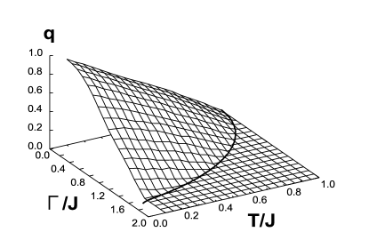
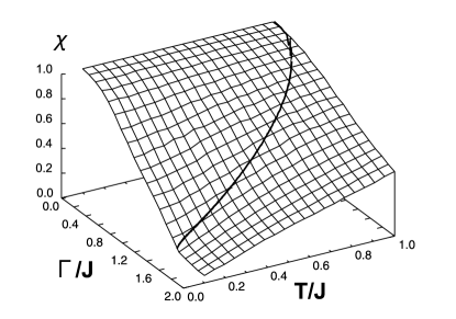
Figure 2: Spin glass order parameters $q$ and $\chi$ from saddle point equations. The frequency summation is taken up to $m=4$. The bold line denotes the phase boundary.

III.4 Improved Landau expansion at quantum regime

At low temperature the static approximation is not justified and we must use a different method. Introducing the auxiliary variables for the expression (34), we write the last term in a linearized form

$$\exp\left[\frac{J^{2}}{2}\sum_{a=1}^{n}\int_{\tau,\tau^{\prime}}\tilde{\chi}(\tau,\tau^{\prime})n^{a}_{z}(\tau)n^{a}_{z}(\tau^{\prime})\right]$$

$$=\int{\cal D}\tilde{z}\exp\left[-\frac{1}{2}\sum_{a}\int_{\tau,\tau^{\prime}}\tilde{z}_{a}(\tau)\chi^{-1}(\tau-\tau^{\prime})\tilde{z}_{a}(\tau^{\prime})+J\sum_{a}\int_{\tau}\tilde{z}_{a}(\tau)n^{a}_{z}(\tau)\right].$$ (43)

As we analyzed in the Landau expansion $\chi(\tau)$ decays exponentially in time at $\tau=0$ and $\beta$. This decay rate is large at low temperature and we can use the instantaneous approximation. Using the derivative expansion for $\tilde{z}(\tau)$, we obtain

$$\int{\cal D}\tilde{z}\exp\left[-\frac{1}{2}\sum_{a}\int_{\tau,\tau^{\prime}}\tilde{z}_{a}(\tau)\chi^{-1}(\tau-\tau^{\prime})\tilde{z}_{a}(\tau^{\prime})\right]\sim\exp\left[-\frac{1}{2\beta\chi}\sum_{a}\int_{\tau}\tilde{z}_{a}^{2}(\tau)-\frac{\chi_{2}}{4\beta^{2}\chi^{2}}\sum_{a}\int_{\tau}(\partial_{\tau}\tilde{z}_{a})^{2}(\tau)\right],$$ (44)

where

$$\chi=\frac{1}{\beta}\int_{\tau}\chi(\tau),\quad\chi_{2}=\frac{1}{\beta}\int_{\tau}\tau^{2}\chi(\tau).$$ (45)

$\chi_{2}$ can be written as $\chi_{2}=-\partial_{\omega}^{2}\chi(\omega)|_{\omega=0}$ and we see that this contribution was not taken into account in the previous approximation. Assuming the form $\chi(\tau)\sim e^{-2h^{\prime}\tau}+e^{-2h^{\prime}(\beta-\tau)}$ we can write $\chi_{2}\sim(\beta\chi)^{3}/2$. The auxiliary variables are integrated out to give

$$\int{\cal D}\tilde{z}\exp\left[-\frac{1}{2\beta\chi}\sum_{a}\int_{\tau}\tilde{z}_{a}^{2}(\tau)-\frac{\chi_{2}}{4\beta^{2}\chi^{2}}\sum_{a}\int_{\tau}(\partial_{\tau}\tilde{z}_{a})^{2}(\tau)+J\sum_{a}\int_{\tau}\tilde{z}_{a}(\tau)n^{a}_{z}(\tau)\right]$$

$$=\exp\left[\frac{J^{2}}{2}\sum_{a}\int_{\tau}G(\tau-\tau^{\prime})n_{z}^{a}(\tau)n_{z}^{a}(\tau^{\prime})\right],$$ (46)

where

$$G(\tau)=\sum_{n\neq 0}\frac{\chi^{-1}}{(\pi n)^{2}+\chi^{-2}}e^{-2\pi in\tau/\beta}.$$ (47)

Compared to Eq.(43) we find that $\tilde{\chi}(\tau)$ is replaced by $G(\tau)$. Then the correlation function of $n_{z}^{a}(\tau)n_{z}^{a}(\tau^{\prime})$ in Eq.(46) is calculated by the gauge transformation as $D_{h_{a}}(\tau-\tau^{\prime})\Gamma^{2}/h_{a}^{2}$. Taking the limit $n\to 0$, we obtain approximately

$$\beta f_{\rm eff}=\frac{\beta^{2}J^{2}}{4}(\chi^{2}-q^{2})-\int Dz_{1}\ln\left[\int Dz_{2}(e^{\beta h}+e^{-\beta h})\right]-\frac{\beta^{2}J^{2}}{2}\int Dz_{1}D^{\prime}z_{2}\frac{\Gamma^{2}}{h^{2}}\frac{\chi}{1+\beta h\chi}.$$ (48)

This effective free energy is valid at low temperature and the phase transition point at $T=0$ can be determined from

$$\beta J\chi=\frac{1}{\beta J\chi}\left(\int D^{\prime}zz^{2}-1\right)+\frac{\beta J}{2}\int D^{\prime}z\left(z^{2}-\int D^{\prime}z^{\prime}z^{\prime 2}\right)\frac{\Gamma^{2}}{h^{2}}\frac{1}{1+\beta h\chi},$$

$$1=\frac{1}{(\beta J\chi)^{2}}\left(\int D^{\prime}zz^{2}-1\right)^{2}.$$ (49)

These equations have the solution $\beta J\chi\sim 0.62$ and $\Gamma/J\sim 1.62$ at $T\to 0$. We see in Fig.1 that the result of the quantum regime is smoothly connected to that of the classical regime.

Finally we determine the boundary between the classical and quantum regime. According to Eq.(47), the time dependence becomes important when the first Matsubara frequency is comparable to the “mass” term of the propagator. Thus we identify the quantum regime $\pi\chi\$$\stackrel{{\scriptstyle\textstyle<}}{{\sim}}$$\,\ 1$ which is illustrated in Fig.1.

IV Conclusions

We have discussed quantum random spin systems using the field theoretical method based on the spin coherent state representation. The partition function is represented as a functional integral and the continuous integration variables describe the spin motion on a unit sphere. This formulation can be applied to arbitrary Hamiltonians with arbitrary spin $S$.

In previous works for the Ising spin ($S=1/2$) systems, the eigenstates of $\hat{S}_{3}$ has been used for the closure relation to be inserted into the Trotter decomposition. This formulation gives discrete integration variables and the continuum limit in the time direction cannot be taken since the time derivative for the discrete variables is ill defined. In this sense our formulation is natural and useful even for the Ising systems.

Our method is also useful for explicit calculations. We can use various field theoretical techniques such as the semiclassical method and the gauge transformation. As an application we considered the transverse SK model. The classical effective free energy renormalized by quantum fluctuation effects are expressed in terms of order parameters and the saddle point equations are solved to obtain the phase diagram. We showed that the time dependence of $\chi$ is important to obtain the result. We found the quantum phase transition point located between the perturbative and the static results. Our estimate is $\Gamma/J=1.62$ at $T=0$ and is close to the values obtained by others. YI ; MH ; RGAR

What is conceptually important in our calculation is that the role of the order parameter variables is distinguished between the static and nonstatic parts. The order parameter is defined as the static part of the variable and the nonstatic part are integrated out to find the effective classical theory, which is reminiscent of the renormalization group theory. Therefore, it is a straightforward extension to consider the renormalization group calculation as was discussed in Ref.RSY, . Allowing for the spatial fluctuations of the order parameters, we can examine the stability of the critical states and calculate the critical exponents.

We clarified in the present paper the role of the quantum fluctuations using the simple transverse Ising spin glass model. It is a straightforward task to apply our results to other models. For example we can consider the transverse SK model with arbitrary spin $S$. In that case, it is not difficult to calculate the correlation function corresponding to Eq.(10). When $S$ is large, we find that the time dependence becomes weak and the static approximation becomes a good one. In a similar reason, the static approximation is justified when we have an infinite many-body interaction. re These observations show that the present transverse Ising spin model is the simplest one but the quantum effect is maximum. We think the next simplest nontrivial application of our method is the quantum Heisenberg model. Most of the previous works relied on a semiclassical method such as the static approximation BM ; GL2 and the large-$N$ limit SYGPS . We hope that our approach will be useful for studying the quantum effects.

Finally we mention another possible application. In the present paper we considered the imaginary time formulation to calculate the partition function. It is also possible to consider the real time formulation which allows us to analyze the dynamical correlations. This can be done by using the Keldysh formulation. Keldysh We can calculate the dynamical correlation function without using the analytic continuation from imaginary to real time. The Keldysh method is also useful when we consider the random averaging and field theoretical methods were developed for disordered Fermion systems. Kdiss The application to the random quantum spin systems is an interesting problem and is left for future work.

Appendix A Derivation of the saddle point equations

We consider the derivative of the following functions to derive the saddle point equations:

$$F=\int Dz_{1}\ln\left[\int Dz_{2}f(h)\right],\quad G=\int Dz_{1}\frac{\int Dz_{2}f(h)g(h)}{\int Dz_{2}f(h)},$$ (50)

where $h=\left(\Gamma^{2}+M^{2}\right)^{1/2}$ with $M=J(\sqrt{q}z_{1}+\sqrt{\chi-q}z_{2})$. After taking the derivative with respect to $\chi$ or $q$, we take the limit $q=0$. First, we consider the derivative with respect to $\chi$. We have

$$\frac{\partial F}{\partial\chi} = \frac{J}{2}\int Dz_{1}\frac{\int Dz_{2}\frac{z_{2}}{\sqrt{\chi-q}}\frac{\partial}{\partial M}f(h)}{\int Dz_{2}f(h)}$$ (51)

$$= \frac{J}{2}\int Dz_{1}\frac{\int Dz_{2}\frac{1}{\sqrt{\chi-q}}\frac{\partial}{\partial z_{2}}\frac{\partial}{\partial M}f(h)}{\int Dz_{2}f(h)}$$ (52)

$$= \frac{J^{2}}{2}\int Dz_{1}\frac{\int Dz_{2}\frac{\partial^{2}}{\partial M^{2}}f(h)}{\int Dz_{2}f(h)},$$ (53)

where we referred the definition of the integration measure (35) to use $ze^{-z^{2}/2}=-de^{-z^{2}/2}/dz$ and the partial integration in the second line. In the same way, we have

$$\frac{\partial G}{\partial\chi}=\frac{J^{2}}{2}\int Dz_{1}\left[\frac{\int Dz_{2}\frac{\partial^{2}}{\partial M^{2}}f(h)g(h)}{\int Dz_{2}f(h)}-\frac{\int Dz_{2}\frac{\partial^{2}}{\partial M^{2}}f(h)}{\int Dz_{2}f(h)}\frac{\int Dz_{2}f(h)g(h)}{\int Dz_{2}f(h)}\right].$$ (54)

At the limit $q=0$, $h$ becomes independent of $z_{1}$ and we obtain

$$\left.\frac{\partial F}{\partial\chi}\right|_{q=0} = \frac{1}{2\chi}\frac{\int Dz(z^{2}-1)f(h)}{\int Dzf(h)},$$ (55)

$$\left.\frac{\partial G}{\partial\chi}\right|_{q=0} = \frac{1}{2\chi}\left[\frac{\int Dz(z^{2}-1)f(h)g(h)}{\int Dzf(h)}-\frac{\int Dz(z^{2}-1)f(h)}{\int Dzf(h)}\frac{\int Dzf(h)g(h)}{\int Dzf(h)}\right],$$ (56)

where $M=J\sqrt{\chi}z$. We replaced the derivative with respect to $M$ by that with respect to $z$ and used again the partial integration. In the same way, we obtain

$$\left.\frac{\partial F}{\partial q}\right|_{q=0} = -\frac{1}{2\chi}\left[\frac{\int Dzzf(h)}{\int Dzf(h)}\right]^{2},$$ (57)

$$\left.\frac{\partial^{2}F}{\partial q^{2}}\right|_{q=0} = -\frac{1}{2\chi^{2}}\left[\frac{\int Dz(z^{2}-1)f(h)}{\int Dzf(h)}\right]^{2},$$ (58)

$$\left.\frac{\partial G}{\partial q}\right|_{q=0} = 0,$$ (59)

$$\left.\frac{\partial^{2}G}{\partial q^{2}}\right|_{q=0} = -\frac{1}{\chi^{2}}\frac{\int Dz(z^{2}-1)f(h)}{\int Dzf(h)}\left[\frac{\int Dzz^{2}f(h)g(h)}{\int Dzf(h)}-\frac{\int Dzz^{2}f(h)}{\int Dzf(h)}\frac{\int Dzf(h)g(h)}{\int Dzf(h)}\right].$$ (60)

References

• (1) M. Mézard, G. Parisi, and M.A. Virasoro, Spin Glass Theory and Beyond (World Scientific, Singapore, 1987).
• (2) H. Nishimori, Statistical Physics of Spin Glasses and Information Processing: An Introduction (Oxford University Press, Oxford, 2001).
• (3) S.F. Edwards and P.W. Anderson, J. Phys. F: Met. Phys. 5, 965 (1975).
• (4) D. Sherrington and S. Kirkpatrick, Phys. Rev. Lett. 35, 1792 (1975).
• (5) B.S. Chakrabarti, A. Dutta, and P. Sen, Quantum Ising Phases and Transitions in Transverse Ising Models (Springer, Berlin, 1996).
• (6) A.J. Bray and M.A. Moore, J. Phys. C 13, L655 (1980).
• (7) See for example, S. Sachdev, Quantum Phase Transitions (Cambridge University Press, Cambridge, 1999).
• (8) H. Ishii and T. Yamamoto, J. Phys. C 18, 6225 (1986).
• (9) K.D. Usadel, Solid State Commun. 58, 629 (1986).
• (10) T. Yamamoto and H. Ishii, J. Phys. C 20, 6053 (1987).
• (11) K. Walasek and K. Lukierska-Walasek, Phys. Rev. B 38, 725 (1988).
• (12) T. Yokota, Phys. Rev. B 40, 9321 (1989).
• (13) D. Thirumalai, Q. Li, and T.R. Kirkpatrick, J. Phys. A 22, 3339 (1989).
• (14) Y.Y. Goldschmidt and P.Y. Lai, Phys. Rev. Lett. 64, 2467 (1990).
• (15) K.D. Usadel, G. Büttner, and T.K. Kopeć, Phys. Rev. B 44, 12583 (1991).
• (16) J. Miller and D.A. Huse, Phys. Rev. Lett. 70, 3147 (1993).
• (17) M.J. Rozenberg and D.R. Grempel, Phys. Rev. Lett. 81, 2550 (1998); L. Arrachea and M.J. Rozenberg, ibid. 86, 5172 (2001).
• (18) D.H. Kim and J.J. Kim, Phys. Rev. B 66, 054432 (2002).
• (19) H.F. Trotter, Proc. Am. Math. Soc. 10, 545 (1959); M. Suzuki, Prog. Theor. Phys. 56, 1454 (1976).
• (20) S. Sachdev and J. Ye, Phys. Rev. Lett. 70, 3339 (1993); A. Georges, O. Parcollet, and S. Sachdev, ibid. 85, 840 (2000).
• (21) J.R. Klauder, Phys. Rev. D 19, 2349 (1979).
• (22) J.R. Klauder and B-S. Skagerstam, Coherent States (World Scientific, Singapore, 1985).
• (23) P.B. Wiegmann, Phys. Rev. Lett. 60, 821 (1988); E. Fradkin and M. Stone, Phys. Rev. B 38, 7215 (1988).
• (24) A. Alscher and H. Grabert, J. Phys. A 32, 4907 (1999).
• (25) M. Stone, Phys. Rev. D 33, 1191 (1986); K. Fujikawa, ibid. 73, 025017 (2006).
• (26) J. Ye, S. Sachdev, and N. Read, Phys. Rev. Lett. 70, 4011 (1993); N. Read, S. Sachdev, and J. Ye, Phys. Rev. B 52, 384 (1995).
• (27) G. Parisi, Phys. Rev. Lett. 43, 1754 (1979); J. Phys. A 13, L115 (1980); 13, L1101 (1980); 13, L1887 (1980).
• (28) Y.Y. Goldschmidt, Phys. Rev. B 41, 4858 (1990); T. Obuchi, H. Nishimori, and D. Sherrington, J. Phys. Soc. Jpn. 75, 054002 (2007).
• (29) Y.Y. Goldschmidt and P.Y. Lai, Phys. Rev. B 43, 11434 (1991).
• (30) L.V. Keldysh, Sov. Phys. JETP 20, 1018 (1965); See for Fermion systems, J. Rammer and H. Smith, Rev. Mod. Phys. 58, 323 (1986); For spin systems, M.N. Kiselev and R. Oppermann, Phys. Rev. Lett. 85, 5631 (2000).
• (31) A. Kamenev and A.V. Andreev, Phys. Rev. B 60, 2218 (1999); C. Chamon, A.W.W. Ludwig, and C. Nayak, ibid. 60, 2239 (1999).