A Comprehensive Analysis of Swift/XRT Data:
III. Jet Break Candidates in X-ray and Optical Afterglow Lightcurves

Abstract

The Swift/XRT data of 179 GRBs (from 050124 to 070129) and the optical afterglow data of 57 pre- and post-Swift GRBs are analyzed, in order to investigate jet-like breaks in the afterglow lightcurves. Using progressively rigorous definitions of jet breaks, we explore whether the observed breaks in the X-ray and optical lightcurves can be interpreted as a jet break, and their implications in understanding GRB energetics if these breaks are jet breaks. We find that not a single burst can be included in the “Platinum” sample, in which the data satisfy all the criteria needed to define a jet break, i.e. a clear achromatic break observed in both the X-ray and optical bands, and that the pre- and post-break decay segments satisfy the closure relations in the same, simplest jet model. However, by releasing one or more requirements to define a jet break, some jet-break candidates of various degrees could be identified. In the X-ray band, 42 out of the 103 well-sampled X-ray lightcurves have a decay slope of the post-break segment $\gtrsim 1.5$ (“Bronze” sample), and 27 of them also satisfy the closure relations of the forward shock models for both the pre- and post- break segments (“Silver” sample). The numbers of the “Bronze” and “Silver” candidates in the optical lightcurves are 27 and 23, respectively. Thirteen bursts have well-sampled optical and X-ray lightcurves, but only seven cases are consistent with an achromatic break, but even in these cases only one band satisfies the closure relations (“Gold” sample). The breaks in other GRBs are all chromatic. The observed break time in the XRT lightcurves is statistically earlier than that in the optical bands. All these raise great concerns in interpreting jet-like breaks as jet breaks and further inferring GRB energetics from these breaks. On the other hand, if one assumes that these breaks are jet breaks, one can proceed to perform a similar analysis as previous work to study GRB collimation and energetics. We have performed such an analysis with the “Silver” and “Gold” jet break candidates. We calculate the jet opening angle ($\theta_{j}$) and kinetic energy ($E_{K}$) or their lower limits with the ISM forward shock models using the X-ray afterglow data. The derived $E_{K}$ distribution reveals a much larger scatter than the pre-Swift sample. A tentative anti-correlation between $\theta_{j}$ and $E_{\rm K,iso}$ is found for both the pre-Swift and Swift GRBs, indicating that the $E_{K}$ could still be quasi-universal, if the breaks in discussion are indeed jet breaks.

1 Introduction

Swift, a multi-wavelength gamma-ray burst (GRB) mission (Gehrels et al. 2004), has led to great progress in understanding the nature of the GRB phenomenon (see recent reviews by Mészáros 2006; Zhang 2007). One remarkable advance from Swift is that the on-board X-ray telescope (XRT; Burrows et al. 2005a) has established a large sample of X-ray lightcurves from tens of seconds to days, sometimes even months (e.g. GRB 060729, Grupe et al. 2006) after the GRB triggers, and revealed a canonical X-ray lightcurve that is composed of four successive power-law decaying segments (Zhang et al. 2006; Nousek et al. 2006; O’Brien et al. 2006a) with superimposing erratic flares (Burrows et al. 2005b). These segments include a GRB tail segment (Segment 1, with a decay slope $\alpha_{1}>2$), a shallow decay segment (Segment 2, $\alpha_{2}<0.75$), a normal decay segment (Segment 3, $\alpha_{3}\sim 1$), and a jet-like decay segment (Segment 4, $\alpha_{4}>1.5$). The GRB tail and the shallow decay segment are usually seen in the XRT lightcurves (O’Brien et al. 2006a; Liang et al. 2006; Willingale et al. 2007; Zhang et al. 2007c, hereafter Paper I; Liang et al. 2007, hereafter Paper II). The jet-like decay segment, however, has occasionally been observed, but only for a small fraction of bursts (Burrows & Racusin 2007; Covino et al. 2006). Some bursts were observed with Swift/XRT and/or Chandra for weeks and even months after the GRB triggers, with no evidence of detecting a jet break in their X-ray lightcurves (Grupe et al. 2006; Sato 2007).

The jet models had been extensively studied in the pre-Swift era (e.g., Rhoads 1999, Sari et al. 1999; Huang et al. 2000; see reviews by Mészáros 2002; Zhang & Mészáros 2004; Piran 2005). An achromatic break is expected to be observed in multi-wavelength afterglow lightcurves at a time when the ejecta are decelerated by the ambient medium down to a bulk Lorentz factor $\sim 1/\theta_{j}$, where $\theta_{j}$ is the jet opening angle (Rhoads 1999; Sari et al. 1999). Most GRBs localized in the pre-Swift era with deep and long optical monitoring have a jet-like break in their optical afterglow lightcurves (see Frail et al. 2001; Bloom, Frail, & Kulkarni 2003; Liang & Zhang 2005 and the references therein), but the achromaticity of these breaks was not confirmed outside of the optical band. Panaitescu (2007) and Kocevski & Butler (2007) studied the jet breaks and the jet energy with the XRT data. However, the lack of detection of a jet-like break in most XRT lightcurves challenges the jet models, if both the optical and X-ray afterglows are radiated by the forward shocks. Multiwavelength observational campaigns raise the concerns that some jet-break candidates may not be achromatic (Burrows & Racusin 2007; Covino et al. 2006, cf. Dai et al. 2007; Curran et al. 2007). Issues regarding the nature of previous “jet breaks” have been raised (e.g. Zhang 2007).

The observational puzzles require a systematical analysis on both the X-ray and the optical data. This is the primary goal of this paper. We analyze the Swift/XRT data of 179 GRBs (from 050124 to 070129) and the optical afterglow data of 57 pre-Swift and Swift GRBs, in order to systematically investigate the jet-like breaks in the X-ray and optical afterglow lightcurves (§2). We measure a jet break candidate from the data with a uniform method and grade the consistency of these breaks with the forward shock models (§3), then compare these breaks observed in the X-ray and optical lightcurves (§4). Assuming that these breaks are real jet breaks, we revisit the GRB jet energy budget (Frail et al. 2001; Bloom et al. 2003; Berger et al. 2003) with the conventional jet models (§5). Conclusions and discussion are presented in §6. Throughout this paper the cosmological parameters $H_{0}=71$ km s^-1 Mpc^-1, $\Omega_{M}=0.3$, and $\Omega_{\Lambda}=0.7$ are adopted.

2 Data

The XRT data are taken from the Swift data archive. We have developed a script to automatically download and maintain all the XRT data. The HEAsoft packages, including XSPEC, XSELECT, XIMAGE, and Swift data analysis tools, are used for the data reduction. We have developed an IDL code to automatically process the XRT data for a given burst in any user-specified time interval. For details of our code please see Papers I and II.

We process all the XRT data (179 bursts) observed between 2005 January and 2007 January with our tools. We are only concerned with the power-law afterglow segments 2, 3, & 4 without considering the steep decay segment (1) and the flares in the lightcurves. Since the flares are generally superimposed upon the underlying afterglows (Chincarini et al. 2007) and their spectral properties are different from those of the power-law decaying afterglows (Falcone et al. 2007), we do not consider the afterglow phases with significant flares. First, we inspect the XRT lightcurve of each burst and specify the time interval(s) that we use to derive the spectral and temporal properties. Then, we fit the lightcurve in this time interval with a power-law-like model as presented below. We regard that a lightcurve in the specified time interval does not have significant flares, if the reduced $\chi^{2}$ of the power law fits is less than 2. We obtain a sample of 103 XRT lightcurves that have a good temporal coverage without significant flares.

We fit the lightcurve in the specified time interval to derive the decay slopes of the three segments and the two breaks, $t_{b,1}$ (the shallow to normal transition break, possibly due to cessation of energy injection in the forward shock; Paper II) and $t_{b,2}$ (the normal to steep transition break, possibly a jet break). Physically, these breaks should be smooth (e.g., Panaitescu & Mészáros 1999; Moderski et al. 2000; Kumar & Panaitescu 2000; Wei & Lu 2000). As shown in Paper II, the energy injection break is usually seen in the XRT lightcurves, and a smoothly broken power law (SBPL) model fits most XRT lightcurves well, which is defined as

$$f=f_{0}\left[\left(\frac{t}{t_{\rm b,1}}\right)^{\omega_{1}\alpha_{2}}+\left(\frac{t}{t_{\rm b,1}}\right)^{\omega_{1}\alpha_{3}}\right]^{-1/\omega_{1}},$$ (1)

where $\omega_{1}$ describes the sharpness of the break at $t_{\rm b,1}$, with a larger value corresponding to a sharper break. If the jet-like decay segment is also observed, the lightcurve break near $t_{b,2}$ evolves as

$$f_{j}=f_{0}\left[\left(\frac{t_{j}}{t_{\rm b,1}}\right)^{\omega_{1}\alpha_{2}}+\left(\frac{t_{j}}{t_{\rm b,1}}\right)^{\omega_{1}\alpha_{3}}\right]^{-1/\omega_{1}}\left(\frac{t}{t_{b,2}}\right)^{-\alpha_{4}}.$$ (2)

Therefore, a three-segment XRT afterglow lightcurve should be fitted with a smoothed triple power law (STPL) model,

$$F=(f^{-\omega_{2}}+f_{j}^{-\omega_{2}})^{-1/\omega_{2}}$$ (3)

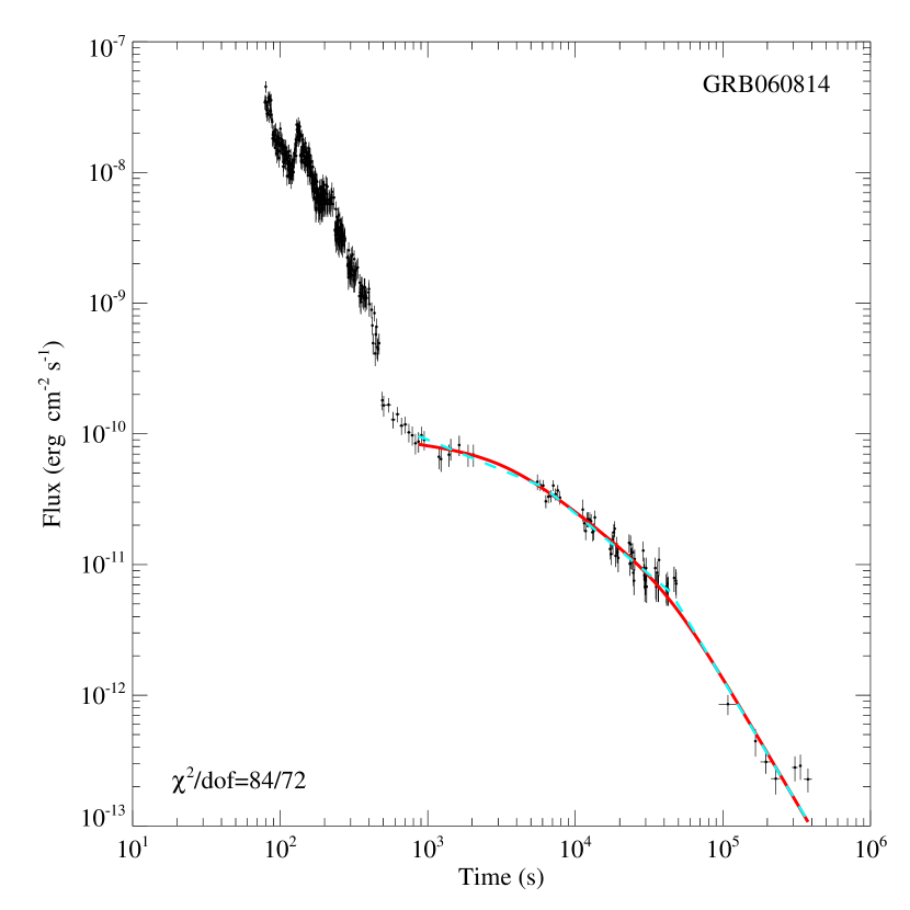
Figure 1: Comparison of the fitting results with the STPL (solid line) and the JTPL(dashed) models. The last three data points are excluded in the fits.

where $\omega_{2}$ is the sharpness factor of the jet break at $t_{b,2}$. At $t\ll t_{\rm b,1}$, the lightcurve is dominated by the shallow decay phase, $F\sim(t/t_{\rm b,1})^{-\alpha_{2}}$, and at $t\gg t_{\rm b,2}$, the lightcurve decays as $F\sim(t/t_{\rm b,2})^{-\alpha_{4}}$. As shown in Paper II, $t_{b,1}$ and $t_{b,2}$ are not significantly affected by $\omega_{1}$ and $\omega_{2}$, but $\alpha_{3}$ is. The normal decay segment can be smeared by both the pre- and post- segments if $\omega_{1}$ and $\omega_{2}$ are small ($<1$). We find that $\omega_{1}=\omega_{2}=3$ can well identify the breaks in the lightcurves. Taking the XRT lightcurve for GRB 060814 as an example, in Fig.1 we compare the fit curve of the STPL model with a simpler fit by a joint triple power law (JTPL) model, which is defined as

$$F=f_{0}\cases{t^{-\alpha_{2}},&$t<t_{b,1}$,\cr t_{b,1}^{\alpha_{3}-\alpha_{2}}t^{-\alpha_{3}},&$t_{b,1}\leqslant t\leqslant t_{b,2}$,\cr t_{b,1}^{\alpha_{3}-\alpha_{2}}t_{b,2}^{\alpha_{4}-\alpha_{3}}t^{-\alpha_{4}},&$t>t_{b,2}$.\cr}$$ (4)

We find that the breaks at $\sim 3.4$ ks and $\sim 40$ ks are well identified in both models, and the results are consistent with each other. On the other hand, the STPL model is smooth without sharp breaks (Fig.1), coinciding more within the physical context of these breaks. The fitting result of the JTPL model strongly depends on the initial values of the two breaks. The results may be misleading, especially when the normal decay phase lasts only a very short time (in log-scale). Therefore, we use the STPL model and fix $\omega_{1}=\omega_{2}=3$ throughout this analysis.

The jet break signature may not be obvious, therefore we use the following strategy to select the best model among the STPL, SBPL, and single power law (SPL) models to fit the XRT lightcurves. In the sense of Occam’s Razor, the simplest model should be adopted. On ther other hand, in order to avoid missing a jet break in the lightcurves, we accept a fit model as the best one when the derived breaks are sufficiently constrained by the data (i.e. $\delta t_{b}<t_{b}$, where $\delta t_{b}$ is the fitting error of $t_{b}$, even if the $\chi^{2}$ is not significantly improved when compared to a simpler model). We thus first fit the lightcurves with the STPL model (Eq. [3]). This model is a reasonable fit to all of the lightcurves. In case of $\delta t_{b}<t_{b}$, we suggest that such a lightcurve has three segments and we adopt the STPL model fit. We find that only 6 lightcurves satisfy this criterion (see Table 1). We fit the remaining lightcurves with the SBPL model (Eq. [1]), and similarly we examine whether or not $t_{b,1}$ is sufficiently constrained. The SBPL fits are adopted for 78 lightcurves. We fit the remaining lightcurves (26 bursts) with the SPL model. Please note that, as shown in Paper II, the sharp breaks in GRBs 060413, 060522, 060607A, and 070110 are possibly not of external origin (see also Troja et al. 2007). We do not include these sharp breaks in this analysis. GRB 060522 and 070110 have a normal decay segment after an abnormally sharp lightcurve break, therefore we fit this post-break region to a simple power law. GRB 061202 shows significant spectral evolution throughout its lightcurve, so we do not consider this burst either. Our full resulting fits are summarized in Table 1. Using the time intervals defined by the fitting results, we extract the spectrum of each segment, and fit it with a simple power law model with absorption by both our Galaxy and the host galaxy. The spectral fitting results are also reported in Table 1.

In order to compare the X-ray break candidates with the optical lightcurves, we also perform an extensive analysis of the optical lightcurves for both pre-Swift and Swift bursts. We search for the optical afterglow data in the literature and compile a sample of 57 optical lightcurves that have a good temporal coverage. These lightcurves are fit with the same strategy as that for the XRT lightcurves. The fitting results are reported in Table 2.

3 Jet Break Candidates in the X-Ray and Optical Lightcurves

A break with $\Delta\alpha\sim 1$ is predicted by the forward shock jet models. Since it is purely due to dynamic effects, it should be achromatic with no spectral evolution across the break, and both the pre- and post-break segments should also be consistent with the forward shock models. As shown in Table 2, no significant spectral evolution in the segments 3 and 4 is found for most bursts, and the X-ray spectral index is $\sim 1$ (see also O’Brien et al. 2006b). Assuming that both the optical and the X-ray afterglows are produced by the forward shocks, we select jet break candidates from the results shown in Tables 1 and 2, and grade these candidates as “Bronze”, “Silver”, “Gold”, and “Platinum” based on the consistency of data with the models. The definitions of these grades are summarized in Table 3. A break with a post-break segment being steeper than 1.5 is selected as “Bronze”. It is promoted to “Silver”, if both pre- and post-break segments are consistent with the closure relations of the models. If multiwavelength data are consistent with an achromatic break with only one band satisfies the jet models, a “Silver” Candidate is elevated to “Gold” candidate. If an achromatic break can be established independently at least in two bands with both bands satisfying the jet models, this break is termed as a “Platinum” jet break candidate.

3.1 “Bronze” Jet Break Candidates

We first select the “Bronze” jet break candidates from both the X-ray and optical data shown in Tables 1 and 2. Without multiple wavelength modelling, the closure relations between the spectral index ($\beta=\Gamma-1$) and temporal decay slope of the GRB afterglows present an approach to verify whether or not the data satisfy the models (see Table 1 of Zhang & Mészáros 2004 and references therein, in particular Sari et al. 1998; Chevalier & Li 2000; Dai & Cheng 2001). As shown in our Tables 1 and 2, the observed X-ray and optical spectral indices are larger than 0.5 (except for the optical data of GRB 021004), indicating that the observed X-ray and optical afterglows are usually in the spectral regime of $\nu_{X}>\max(\nu_{m},\nu_{c})$ (Regime I) or $\nu_{m}<\nu_{X}<\nu_{c}$ (Regime II), where $\nu_{c}$ and $\nu_{m}$ are the cooling frequency and the typical frequency of the synchrotron radiation, respectively. In the standard forward shock models, the decay slope of the pre-break segment is $\alpha_{3}=(3\beta_{3}-1)/2$ for emission in the spectral regime I (both ISM and wind) and $\alpha_{3}=3\beta_{3}/2$ (ISM) or $\alpha_{3}=(3\beta_{3}+1)/2$ (wind) for emission in Regime II. After the jet break and assuming maximized sideways expansion of jets, the lightcurve evolves as $\alpha_{4}=2\beta$ (spectral regime I) or $\alpha_{4}=2\beta+1$ (spectral regime II). If the jet sideways expansion effect can be negligible, the post-break decay index $\alpha_{4}$ is shallower, i.e. $\alpha_{4}=\alpha_{3}+0.75$ (ISM) and $\alpha_{4}=\alpha_{3}+0.5$ (wind) (Panaitescu 2005). The observed X-ray spectral indices are greater than 0.5. Therefore, within the ISM forward shock jet model the decay slopes of the pre- and post-break segments of the X-rays in the spectral regime II should be greater than 0.75 and 1.5, respectively (even without significant sideways expansion). The wind model (regime II) and the jet model with maximum sideways expansion would make the slopes even steeper. We therefore pick 1.5 as the critical slope to define the “Bronze” jet break sample. As shown in Tables 1 and 2, 42 breaks of the XRT lightcurves and 27 of the optical lightcurves satisfy the “Bronze” jet break candidate criterion. These lightcurves are shown in Fig. 2. We summarize the data of these breaks in Table 4. Our “Bronze” jet break candidate sample is roughly consistent with that reported by Panaitescu (2007). The jet breaks in the radio afterglow lightcurve of GRBs 970508 (Frail et al.2000) and 000418 (Berger et al. 2001) are also included in our “Bronze” sample.

The criterion of the “Bronze” jet break candidate concerns only the decay slope of the post-break segment. We notice that the lightcurve of the normal-decaying phase declines as $\alpha_{3}=(3\beta+1)/2$ in wind medium, i.e., $\alpha_{3}\sim 2$ for $\beta\sim 1$. As shown in Paper II, some jet-like breaks have a pre-break segment much shallower than that expected from the jet models. A reasonable possibility would be that they are due to the energy injection effect in the forward shock model in the wind medium. Therefore, some “Bronze” jet break candidates may be fake energy injection breaks instead.

3.2 “Silver” Jet Break Candidates

We promote a “Bronze” jet break candidate to the “Silver” sample if both the pre- and post-break segments are consistent with the models in at least one band. The decay slope of the pre-break segment of a jet break for the bursts in our sample should be steeper than 0.75. Fifty-two out of the 71 “Bronze” jet break candidates in Table 4 agree with the “Silver” candidate criterion (29 in the X-ray lightcurves and 23 in the optical light curves). The X-ray light curve of GRB 970828 has a break at $\sim 2.2$ days, with $\alpha_{3}=1.44$, $\alpha_{4}=2.6$, and $\beta_{X}\sim 1$ (Djorgovski et al. 2001). The X-ray lightcurve of GRB 030329 has a break at $0.52\pm 0.05$ days, with $\alpha_{3}=0.87\pm 0.05$, $\alpha_{4}=1.84\pm 0.07$, $\beta_{3}=1.17$, and $\beta_{4}=0.8\pm 0.3$ (Willingale et al. 2004). We include these two pre-Swift GRBs in the X-ray jet break candidate “Silver” sample.

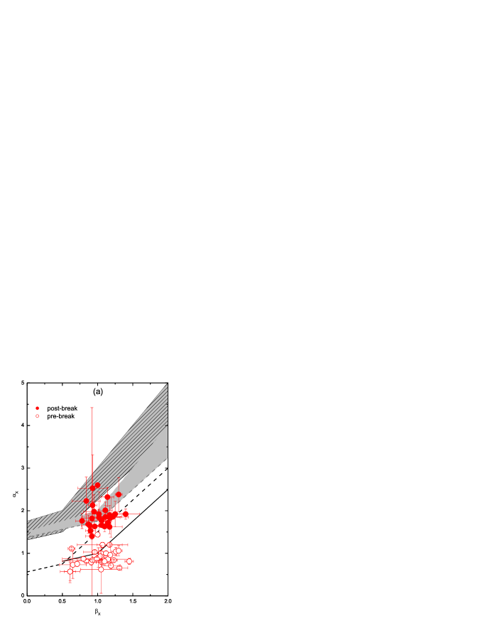
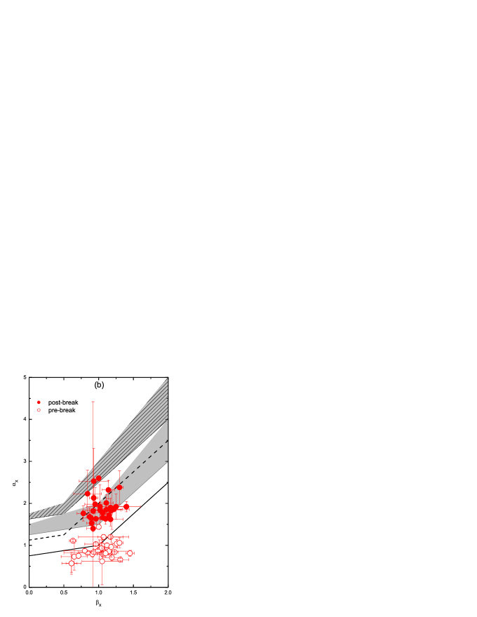
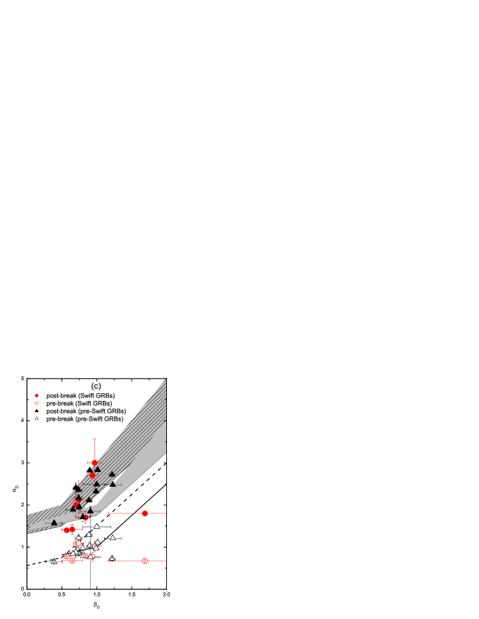
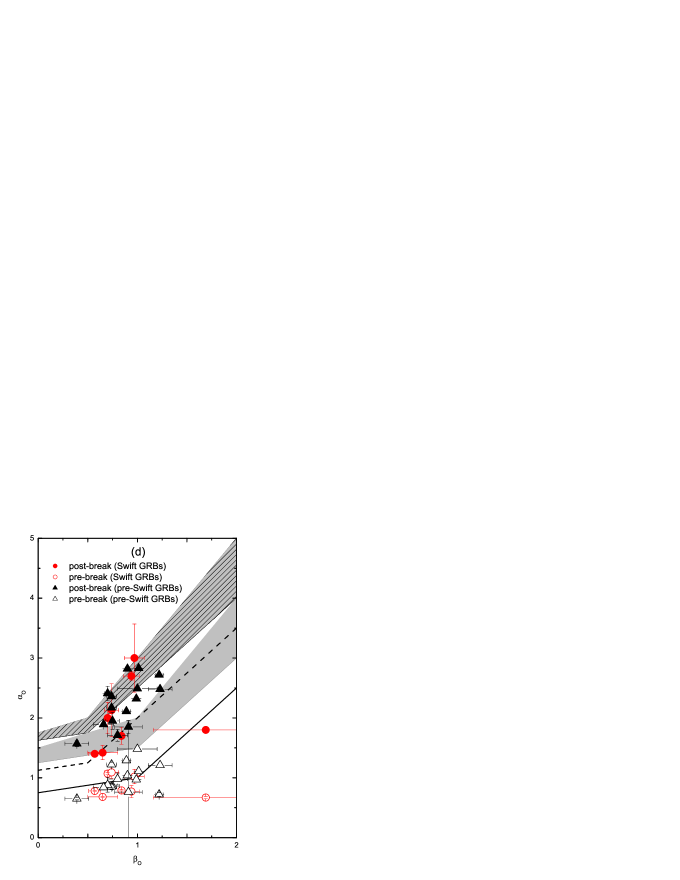
Figure 3: XRT and optical data compared for the “Silver” jet break candidates with the closure relations of the forward shock models for emissions in the spectral regimes (I)$\nu_{X}>\max(\nu_{m},\nu_{c})$ and (II) $\nu_{m}<\nu_{X}<\nu_{c}$. The solid lines and shaded regions indicate the closure relations of the pre- and post-break segments in the spectral regime I. The lower/upper boundaries of the regions are defined with the closure relation without/with taking the jet sideways expansions into account. Similarly, the dashed lines and shaded regions filled with lines are for the emission in the spectral regime II. The open symbols represent the data for the pre-break segments, and the filled symbols for the post-break segment. The circles stand for the Swift GRBs, and triangles for the pre-Swift GRBs. Panel (a): ISM, XRT data; Panel (b): wind, XRT data; Panel (c): ISM, optical data; Panel (d): wind, optical data.

Figure 3 shows the distribution of these bursts in the ($\alpha,\beta$)-plane combined with the closure relations for the models (ISM and wind medium). The X-ray data of the “Silver” jet break candidates are shown in Figs. 3(a) and 3(b). It is found that the X-rays are consistent with the models in the spectral regime I, although the decay slopes of both the pre- and post-break segments are slightly shallower than the model predictions according to the observed spectral indices (see also Willingale et al. 2007; Paper II). As argued in Paper II, this may be due to the simplification of the models. Simulations considering more realistic physical effects, such as energy transitions between different epoches (Kobayashi & Zhang 2007), evolution of microphysics parameters (Panaitescu et al. 2006; Ioka et al. 2005), and jet profiles (Zhang et al. 2004; Yamazaki et al. 2006), could expand the model lines into broad bands, which could accommodate the observational data better.

The data for the “Silver” jet break candidates in the optical band (15 pre-Swift GRBs and 8 Swift GRBs) are shown in Figs. 3(c) and 3(d). Since no time-resolved spectral analysis for the optical data is available, we take the same spectral index for both the pre- and post-break segments. Differing from the X-rays, the optical emission of the post-break segment is consistent with the jet model in the spectral regime II for most bursts. However, the pre-break segment is also shallower than that predicted by the models in this spectral regime.

3.3 “Gold” Jet Break Candidates

A “Gold” jet break candidate requires that the break is achromatic at least in two bands, and that the break should satisfy the criteria of a “Silver” candidate at least in one band. Inspecting the data in Table 4 and the lightcurves in Fig. 2, one approximately achromatic break is observed in both X-ray and the optical lightcurves of GRBs 030329, 050730, 050820A, 051109A, and 060605. The optical afterglows of GRBs 050525A, 060206, 060526, and 060614 are bright, and a jet-like break is clearly observed in their optical lightcurves. Guided by the optical breaks, some authors argued for achromatic breaks in the XRT lightcurves of these GRBs. Without the guidance of the optical lightcurves, one cannot convincingly argue a break in the XRT lightcurves of these GRBs, but the data may be still consistent with the existence of an achromatic break. Both the optical and radio data of GRB 990510 are consistent with the jet models. We inspect the data of these bursts case by case, and finally identify 7 “Gold” candidates, as discussed below.

• GRB 990510: The pre-Swift jet break candidate of GRB 990510 is an exemplar of a jet break (Harrison et al. 1999). The break is achromatic in different colors in the optical band. The radio data post the break is also consistent with the jet models. However, with the radio data alone, one cannot independently claim this break (D. Frail, 2006, personal communication). Therefore, we include this jet candidate in the “Gold” but not “Platinum” category.

• GRB 030329: Its X-ray lightcurve has only five data points. Fitting with the SBPL model shows that $\alpha_{1}=0.96\pm 0.56$, $\alpha_{2}=1.81\pm 0.05$, and $t_{b,X}=30.6\pm 19.3$ ks with $\chi^{2}/{\rm dof}=4.2/1$. The break is consistent with the closure relations, and the $t_{b,X}$ agrees with the $t_{b,O}$ within error scope (see also Willingale et al. 2004). However, the achromaticity of this break is somewhat questionable. The break in the X-ray lightcurve has a great uncertainty since the fit has only one degree of freedom. On the other hand, the fit to the SPL model yields $\alpha=1.72\pm 0.01$ and $\chi^{2}=9.0/3$, indicating that the SBPL fit is required by the data. We cautiously grade this burst to the “Gold” sample with the caveat of sparse X-ray data in mind.

• GRB 050525A: Blustin et al. (2006) fitted the XRT data of GRB 050525A and derived a break at $13.726^{+7.469}_{-5.123}$ ks, with $\alpha_{3}=1.20\pm 0.03$ and $\alpha_{4}=1.62^{+0.11}_{-0.16}$. The break is consistent with being achromatic with the break identified in the optical band. The issue with their fitting is that the $\chi^{2}$ is too small (reduced $\chi^{2}_{r}$ = 0.50 (25 dof)). We increase the signal-to-noise ratio of the data by rebinning the lightcurve, and fit it from 5.94ks to 157.85 ks. We find that a simple power law is the best fit to the data, with a decay slope $1.40\pm 0.05$ ($\chi^{2}_{r}\sim 1$, 11 dof). The decay slope is much larger than that of the normal decay segment($\sim 1$). A jet-like break is likely embedded in the data. We thus adopt the fitting by Blustin et al. (2006) and cautiously include this burst in the “Gold” sample.

• GRB050820A: Its optical lightcurve traces the XRT lightcurves after $10^{4}$ seconds post-burst. An achromatic break at $\sim 4$ days post-burst is observed. Its pre-break segments are well consistent with the models, but the post-break segments are slightly shallower than the prediction of the jet models. We cautiously promote this break to the “Gold” sample.

• GRB 051109A: The break time in both the X-ray and optical lightcurves is $\sim 25$ ks. Although the decay slopes are $\alpha_{X,4}=1.53\pm 0.08$ and $\alpha_{O,4}=1.42\pm 0.12$, slightly shallower than those predicted by the no-spreading jet models according to the observed spectral index, this burst is included in the “Gold” candidate sample, similar to GRB 050820A.

• GRB 060526: The optical lightcurve of GRB 060526 has a significant break at $\sim 1$ day post-burst (Dai et al. 2007). Its X-ray flux after $10^{2}$ ks is very low (with a significance level of detection being lower than 3 $\sigma$). Dai et al. (2007) suggested a jet-like break in the XRT lightcurve by considering the contamination of a nearby source in the field of view. In all our analyses, we do not try to identify a nearby X-ray contamination source for any GRB, so our best fit does not reveal this jet-break within the observational error scope. In view of the analysis of Dai et al. (2007), we also cautiously grade this break in the “Gold” category.

• GRB 060614: After subtracting the contribution of the host galaxy, the optical lightcurve of GRB 060614 shows a clear break at $104$ ks (Della Valle et al. 2006). Mangano et al. (2007) argue that the XRT lightcurve also has a break at this time. Fitting with our STPL cannot reveal this break. However, we note that $\alpha_{4}$ in the X-ray lightcurve of this burst is $\sim 1.9$, consistent with a post-jet-break decay slope. Although a jet-like break cannot be independently claimed at the optical break time with the X-ray data alone, the multi-wavelength data are still consistent with the existence of such a break, with the possibility that the injection break time and the jet break time are close to each other. Therefore, we agree with the suggestion by Mangano et al. (2007) and grade this break as “Gold”.

To be conservative, we do not include GRBs 050730, 060206, and 060605 in our “Gold” candidate sample, as discuss below.

• GRB050730: The break happens at $\sim 10$ ks in both the optical and X-ray bands. The pre-break segment in both the X-ray and optical light curves is much shallower than the forward shock model predictions. We thus do not grade this break as a “Gold” candidate.

• GRB 060605: A tentative break is observed at $\sim 10$ ks in both the optical and X-ray afterglow light curves. However, this break time is uncertain in the optical band because no data point around the break time is available. On the other hand, the decay slope of the pre-break segment is only $\sim 0.5$. Similarly to GRB 050730, it is not considered as a “Gold” candidate.

• GRB 060206: Curran et al. (2007) fitted the XRT data of GRB 060206 in the range between $4$ ks and $10^{3}$ ks after the GRB trigger with the SBPL model, and reported $t_{b}=22^{+2.0}_{-0.8}$ ks, and the decay slopes of pre- and post-break segments are $1.04\pm 0.1$ and $1.40\pm 0.7$, respectively. The reduced $\chi^{2}$ of the fit is 0.79 (63 dof). Fitting with the SPL model, they got a slope of $1.28\pm 0.02$ with a reduced $\chi^{2}=1.0$ (65 dof). The fitting results with the SPL model is more reliable than that of the SBPL model. Also by checking the consistency with the models, we find that the the power law spectral index of the WT mode data $1.26\pm 0.06$ after the break is consistent with the “normal decay” phase rather than the post-jet-break phase. For example, for $\nu_{X}>{\rm max}(\nu_{m},\nu_{c})$, the model-predicted temporal break index in the normal decay phase is $1.39\pm 0.09$, this is well consistent with the data. We therefore do not consider this break as a “Gold” jet break candidate.

3.4 “Platinum” Jet Break Candidates

With our definition, a “Platinum” jet break should be independently claimed in at least two bands which should be achromatic. Furthermore, the temporal decay slopes and spectral indices in both bands should satisfy those required in the simplest jet break models. Since the optical and the X-ray afterglows could be in different spectral regimes (Fig. 3), their lightcurve behaviors may be different (e.g. Sari et al. 1999). However, none of the seven “Gold” candidates can be promoted to the “Platinum” sample due to the various issues discussed above. For some other “Silver” candidates in which a prominent “break” is observed in one band, the lightcurve in the other band curiously evolves independently without showing a signature of break (see §4.4 for more discussion). It is fair to conclude that we still have not found a textbook version of jet break after many years of intense observational campaigns.

4 Comparison between the Jet Break Candidates in the X-ray and Optical Bands

In this section we compare the statistical characteristics of the jet break candidates in the X-ray and optical lightcurves. Our final graded jet break candidates are shown in Table 4. The decay slopes of the pre-break segments of those “Bronze” candidates are much shallower than the prediction of the jet models. We cannot exclude the possibility that some “Bronze” jet break candidates are due to the energy injection effect in the wind medium (Paper II). Therefore, for the following analysis, we do not include the “Bronze” jet break candidates.

4.1 Detection Fraction

As shown above, within the 103 XRT lightcurves with a good temporal coverage, 27 have “Silver” or “Gold” jet break candidates. This fraction is 23/57 for optical lightcurves. The detection fraction of jet break candidates in the XRT lightcurves is significantly lower than that in the optical lightcurves.

4.2 Break Time

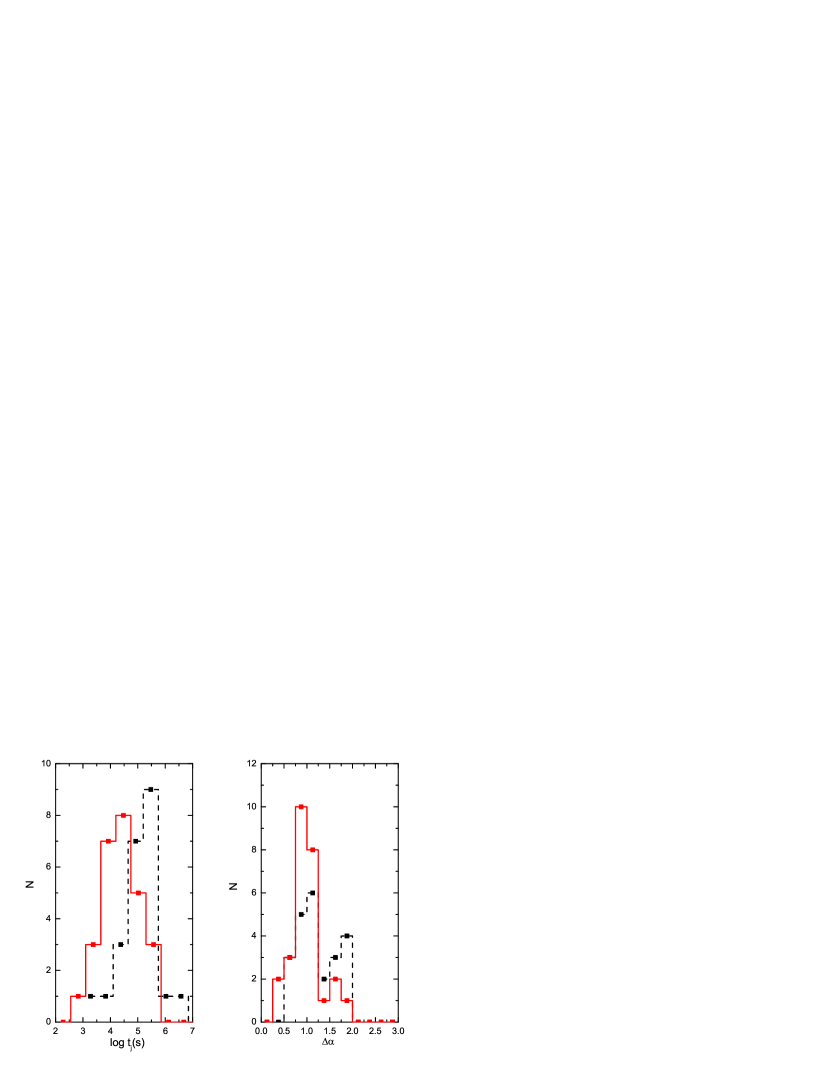
Figure 4: Comparison of the distributions of $t_{j}$ and $\Delta\alpha$ for the XRT data (solid lines) and the optical data (dashed lines).

Figure 4 shows the distributions of $t_{j}$ and $\Delta\alpha$ in the X-ray and optical lightcurves. The distributions of $\log t_{\rm j,X}$/s and $\log t_{\rm j,O}$/s peak at $4.5$ and $\sim 5.5$, respectively. The $t_{\rm j,O}$ distribution has a sharp cutoff right at the high edge of the peak, indicating that the peak is possibly not an intrinsic feature. Since the histogram depends on the bin size selection, we test the normality of the data set with the Shapiro-Wilk normality test. It shows that the probability of a normal distribution for $t_{\rm j,O}$ is $p=11.5\%$ (at 0.05 confidence level), roughly excluding the normality of the distribution. Therefore, this peak is likely due to an observational selection bias. By contrast, the $t_{\rm j,X}$ distribution is log-normal. The Shapiro-Wilk normality test shows $p=79.8\%$ (at confidence level 0.05). These results suggest that the $t_{\rm j,X}$ is systematically smaller than $t_{\rm j,O}$ (see also Kocevski & Butler 2007). This raises the possibility that X-ray breaks and optical breaks may not be physically of the same origin.

4.3 $\Delta\alpha$

With the closure relations of $p>2$ and assuming sideways expansion, we derive $\Delta\alpha=(\beta+1)/2$ for the regime-I ISM model and all the wind models, and $\Delta\alpha=\beta/2+1$ for the regime II ISM model. The observed $\beta_{X}$ is $\sim 1$, hence $\Delta\alpha_{X}\sim 1$ or $\Delta\alpha_{X}\sim 1.5$. Figure 4 (right) shows that the $\Delta\alpha_{X}$ distribution peaks at $\sim 1$, which suggests that most X-ray afterglows are consistent with the regime II models (i.e. X-ray is above both $\nu_{m}$ and $\nu_{c}$). The $\Delta\alpha_{O}$ show a tentative bimodal distribution, with two peaks at $\sim 1$ and $\sim 1.7$, roughly corresponding to the regime I ($\nu_{O}>\rm{max}(\nu_{m},\nu_{c})$) and regime II ($\nu_{m}<\nu_{O}<\nu_{c}$) ISM models, respectively.

4.4 Chromaticity

Being achromatic is the critical criterion to claim a break as a jet break. As shown above, the distribution of $t_{\rm j,X}$ is systematically smaller than $t_{\rm j,O}$, which raises the concern of achromaticity of some of these breaks. Monfardini et al. (2006) have raised the concern that some jet-like breaks may not be achromatic. We further check the chromaticity for the jet candidates case by case. We find 13 bursts that have good temporal coverage in both X-ray and optical bands, with a jet break candidate at least in one band. The results are the following.

• The breaks in the X-ray and optical bands are consistent with being achromatic: GRBs 030329, 050525A, 050820A, 051109A, 060526, and 060614.

• The X-ray and optical breaks are at different epochs: GRBs 060206 and 060210

• A “Silver” jet break candidate in the optical band, but no break in the X-ray band: GRBs 051111 and 060729.

• A “Silver” or “Bronze” jet break candidate in the X-ray band, but no break in the optical band: GRBs 050318 (“Silver”), 050802 (“Bronze”), and 060124 (“Silver”).

The ratio of achromatic to chromatic breaks is 6:7, indicating that the achromaticity is not a common feature of these breaks. It is a great issue to claim the chromatic breaks as a jet break. If both the X-ray and optical emissions are from the forward shocks, one can rule out a large fraction (7/13) of these jet break candidates (many are “Silver” candidates) as a jet break! We indicate the achromaticity of the jet break candidates in Table 4. If the above achromatic-to-chromatic ratio is a common value, most of the breaks without multi-wavelength observations (marked with a “?” in Table 4) should be also chromatic. A possible way out to still consider these breaks as jet breaks is to assume that the band (either X-ray or optical) in which the break is detected is from the forward shock, while emission from the other band is either not from the forward shock or some unknown processes have smeared the jet break feature from the forward shock in that band. Such a model does not explicitly exist yet. We therefore suggest that one should be very cautious to claim a jet break, and further infer the GRB energetics from a jet break candidate. We are probably still a long way from understanding GRB collimation and energetics.

5 Constraints on GRB Jet Collimation and Kinetic Energetics

As shown above, the observed chromatic feature is not consistent with the forward shock models, and it is risky to infer GRB collimation and energetics from these data. On the other hand, it may be still illustrative to perform such a study by assuming that “Silver” break candidates are jet breaks due to the following reasons. First, most pre-Swift works related to jet break and GRB energetics (Frail et al. 2001; Bloom et al. 2003; Berger et al. 2003) were carried out with one-band data only. If multi-wavelength data were not available for the Swift bursts, one would still confidently take the post-Swift “Silver” breaks as jet breaks. It is therefore valuable to study this expanded sample and compare the results with the pre-Swift sample. Second, we notice that there is no GRB that shows a “Silver” jet break candidate in both the X-ray and optical bands but at different times. For example, although a chromatic break is observed in both the optical and X-ray lightcurves of GRBs 060206 and 060210, the X-ray break in GRB 060206 ($\alpha_{2}=0.40\pm 0.05$ and $\alpha_{3}=1.26\pm 0.04$) and the optical break in GRB 060210 ($\alpha_{2}=0.04\pm 0.22$ and $\alpha_{3}=1.21\pm 0.05$) are not jet break candidates. On the other hand, the optical afterglow lightcurve of GRB 060729 show a significant jet-like break, but its XRT lightcurve keeps decaying smoothly without a break. The lightcurve behaviors in the optical and X-ray bands for most GRBs are also enormously different (see also Paper II for a discussion of achromaticity of the shallow-to-normal decay transition in many bursts). These facts suggest that the jet-break candidates we see may indeed have a genuine origin, but we are probably far from understanding the lightcurve behaviors of most bursts. In this section, we assume that those “Silver” or “Gold” jet break candidates are jet breaks, and follow the standard forward shock model to constrain jet collimation and kinetic energy of the GRB jets.

5.1 Models

In the standard afterglow models, the isotropic kinetic energy $(E_{\rm K,iso})$ can be derived from the data in the normal decay phase, and the jet kinetic energy $E_{K}$ can be obtained from the jet break information (e.g. Rhoads 1999; Sari et al. 1999; Frail et al. 2001). The models depend on the power law index $p$ of the electron distribution, the spectral regime, and the medium stratification surrounding the bursts (Mészáros & Rees 1993; Sari et al. 1998; Dai & Lu 1998; Chevalier & Li 2000; Dai & Cheng 2001). As shown in Fig. 3, most bursts in our sample (25 out of 29) are consistent with $p>2$. We therefore only consider $p>2$ in this analysis. Essentially all the data are consistent with the ISM model, although in some bursts the wind model cannot be confidently ruled out. On the other hand, interpreting the early afterglow deceleration feature in GRB 060418 (Molinari et al. 2007) requires that the medium is ISM, even at the very early time (Jin & Fan 2007). We therefore consider only the ISM case in this paper.

We use the X-ray afterglow data to calculate $E_{\rm K,iso}$, following the same procedure presented in our previous Paper (Zhang et al. 2007a), which gives

$$E_{\rm K,iso,52} = \left[\frac{\nu F_{\nu}(\nu=10^{18}~{}{\rm Hz})}{5.2\times 10^{-14}~{}{\rm ergs~{}s^{-1}~{}cm^{-2}}}\right]^{4/(p+2)}D_{28}^{8/(p+2)}(1+z)^{-1}t_{d}^{(3p-2)/(p+2)}$$ (5)

$$\times (1+Y)^{4/(p+2)}f_{p}^{-4/(p+2)}\epsilon_{B,-2}^{(2-p)/(p+2)}\epsilon_{e,-1}^{4(1-p)/(p+2)}\nu_{18}{{}^{2(p-2)/(p+2)}}$$

$$\ \ \ \ ({\rm Spectral\ regime\ I})$$

$$E_{\rm K,iso,52} = \left[\frac{\nu F_{\nu}(\nu=10^{18}~{}{\rm Hz})}{6.5\times 10^{-13}~{}{\rm ergs~{}s^{-1}~{}cm^{-2}}}\right]^{4/(p+3)}D_{28}^{8/(p+3)}(1+z)^{-1}t_{d}^{3(p-1)/(p+3)}$$ (6)

$$\times f_{p}^{-4/(p+3)}\epsilon_{B,-2}^{-(p+1)/(p+3)}\epsilon_{e,-1}^{4(1-p)/(p+3)}n^{-2/(p+3)}\nu_{18}{{}^{2(p-3)/(p+3)}}$$

$$\ \ \ \ ({\rm Spectral\ regime\ II})$$

where $\nu f_{\nu}(\nu=10^{18}{\rm Hz})$ is the energy flux at $10^{18}$ Hz (in units of ${\rm ergs~{}s^{-1}~{}cm^{-2}}$) , $z$ the redshift, $D$ the luminosity distance, $f_{p}$ a function of the power law distribution index $p$ (Zhang et al. 2007a), $n$ the density of the ambient medium, $t_{d}$ the time in the observers frame in days, $Y$ the inverse Compton parameter. The convention $Q_{n}=Q(\rm in\ cgs\ units)/10^{n}$ has been adopted.

If the ejecta are conical, the lightcurve shows a break when the bulk Lorentz factor declines down to $\sim\theta^{-1}$ at a time (Rhoads 1999; Sari et al. 1999)

$$t_{j}\sim 0.5{\rm\ days}(\frac{E_{\rm K,iso,52}}{n})^{1/3}(\frac{1+z}{2})(\frac{\theta_{j}}{0.1})^{8/3}.$$ (7)

The jet opening angle can be derived as

$$\theta_{j}\sim 0.17\left(\frac{t_{j}}{1+z}\right)^{3/8}\left(\frac{E_{\rm K,iso,52}}{n}\right)^{-1/8}.$$ (8)

The geometrically corrected kinetic energy is then given by

$$E_{\rm K,52}=E_{\rm K,iso,52}(1-\cos\theta_{j})~{}.$$ (9)

5.2 Results

Thirty Swift GRBs in our sample have redshifts available. Among them 14 bursts have a jet break candidate detection in the optical or X-ray afterglow lightcurves. For those bursts without jet break detections, we take the time of the last XRT observation as the lower limit of the jet break time. We calculate $E_{\rm K,iso}$ and $\theta_{j}$ (or its lower limit) for these bursts, then derive their $E_{\rm K}$ (or lower limits). We use the normal decay phase to identify the spectral regime for each burst using the following method. We define

$$D=|\alpha^{\rm obs}-\alpha(\beta^{\rm obs})|,$$ (10)

$$\delta=\sqrt{(\delta\alpha^{\rm obs})^{2}+[\delta\alpha(\beta^{\rm obs})]^{2}},$$ (11)

where $\alpha^{\rm obs}(\delta\alpha^{\rm obs})$ and $\alpha(\beta^{\rm obs})$ are the temporal decay slopes (errors) from the observations and that predicted from the closure relations using the observed $\beta$, respectively, for the normal decay phase. The ratio $\phi=D/\delta$ reflects the nearness of the data point to the model lines within errors. In the case of $\phi<1$, the data point goes across the corresponding closure relation line. We derive $\phi$ from the data for both the spectral regimes I and II. By comparing the two $\phi$ values, we then assign each burst to the spectral regime with the smaller $\phi$. We find that the X-rays of about two-third of the bursts are in the spectral regime I. Eq.(5) shows that the calculation of $E_{\rm K,iso}$ is independent of $n$ and only weakly depends on $\epsilon_{B}$ and $p$ with the data in this spectral regime. Therefore, this spectral regime is ideal to measure $E_{\rm K}$. The X-rays of about one-third of the bursts are in the spectral regime II. The inferred $E_{\rm K,iso}$ in this spectral regime significantly depends on both $\epsilon_{B}$ and $n$. This makes it complicated to derive $E_{\rm K,iso}$. In this case $\epsilon_{B}$ or $n$ must be very small (e.g. $\epsilon_{B}\lesssim 10^{-3}$ or $n\sim 10^{-2}$ cm^-3) in order to have the cooling frequency above the observed X-rays at $t\sim 1$ day while retaining a reasonable $E_{\rm K,iso}$ (Zhang et al. 2007a). Please note that by keeping $\epsilon_{e}\sim 0.1$, the $Y$ parameter does not increase significantly for a smaller $\epsilon_{B}$ since the Klein-Nishina correction factor $\eta_{2}$ parameter becomes much smaller (Zhang et al. 2007a).

After identifying the appropriate spectral regime, we derive $p$ from the relations between $p$ and the spectral index (Table 5). Most derived $p$’s are greater than 2, except for GRBs 050820A, 060912, and 060926, and we assign $p=2.01$ for these bursts. In our calculation, we fix $n=0.1$ cm^-3 (Frail et al. 2001) and take initial values of $\epsilon_{B}$ and $Y$ as $10^{-4}$ and $2.7$, respectively. We iteratively search for the maximum value of $\epsilon_{B}$ that ensures the X-rays are in the proper spectral regime. Previous broadband fits and statistical analyses suggest that $\epsilon_{e}$ is typically around 0.1 (Wijers & Galama 1999; Panaitescu & Kumar 2002; Yost et al. 2003; Liang et al. 2004; Wu et al. 2004). Therefore we take $\epsilon_{e}=0.1$ for all the bursts. The $E_{\rm K,iso}$ is calculated with the observed energy flux at a given time. After the energy injection is over, $E_{\rm K,iso}$ is a constant in the scenario of an adiabatic decelerating fireball. In principle, one can derive $E_{\rm K,iso}$ at any time $t_{d}$ with Eqs.(5) and (6). We take the flux at a time $\log t=(\log t_{b,2}+\log t_{b,1})/2$. Our results are reported in Table 4.

We calculate $\theta_{j}$ and $E_{\rm K}$ for the pre-Swift GRBs with the same method. We collect the X-ray afterglow data of the pre-Swift GRBs from the literature. The results are shown in Table 5. Eight bursts in Table 5 are included in the sample presented by Frail et al. (2001). Assuming $n=0.1$ cm^-3 and GRB efficiency $\eta=0.2$, Frail et al. (2001) derived the jet opening angles $\theta_{j}$ of these bursts with the observed gamma-ray energy. We compare our results with theirs ($\theta_{j}^{{}^{\prime}}$) in Fig. 5. They are generally consistent with each other. Since our calculations derive $E_{\rm K,iso}$ directly rather than assuming an $\eta$ value, this result indicates that the derivation of $\theta_{j}$ is insensitive to $\eta$, as suggested by the ${-1/8}$ dependence of $E_{\rm K,iso}$ in Eq.(8).

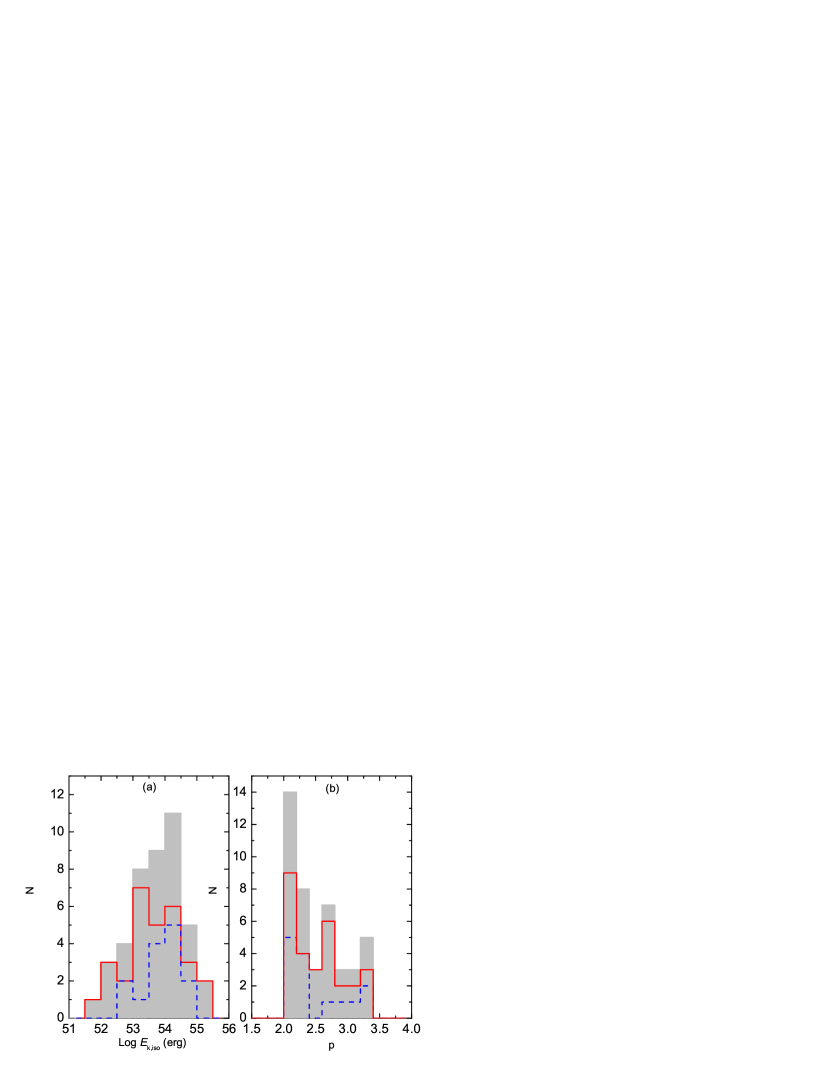
Figure 6: Comparisons of the distributions of $E_{\rm K,iso}$ (panel a) and $p$ (panel b) for Swift GRBs (solid lines) with that of the pre-Swift GRBs (dashed lines). The shaded columns are for both pre-Swift and Swift GRBs combined.

The distributions of $E_{\rm K,iso}$ and $p$ are displayed in Fig. 6. No significant differences between the pre-Swift and the Swift samples are found for these parameters. The Kolmogorov-Smirnov test shows that $p_{K-S}=0.61$ for the $E_{\rm K,iso}$ distribution and $p_{K-S}=0.81$ for the $p$ distribution. As mentioned above, since we only consider $p>2$, the sharp cutoff at $p=2$ is an artifact. A small fraction of bursts might have $p<2$ (such as GRBs 050820A, 060912, and 060926), which would extend the $p$-distribution to smaller values. No evidence for $p$-clustering among bursts is found (see also Shen et al. 2006; Paper II). The $E_{\rm K,iso}$ distribution spans almost 3 orders of magnitude, ranging from $2\times 10^{52}$ to $1\times 10^{55}$ ergs with a log-normal peak at $7\times 10^{53}$ ergs. The probability of the normality is $73\%$ at 0.05 confidence level.

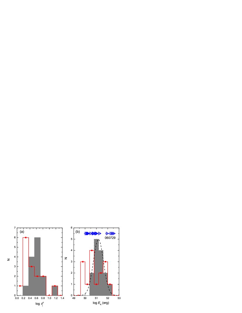
Figure 7: Comparison of the $E_{\rm K}$ distribution of Swift GRBs with that of the pre-Swift GRBs (shaded columns). The lower limits of $E_{\rm K}$ derived from the XRT observations are marked as open triangles. The dashed line is the Gaussian fit to the distribution of $E_{K}$ of pre-Swift GRBs.

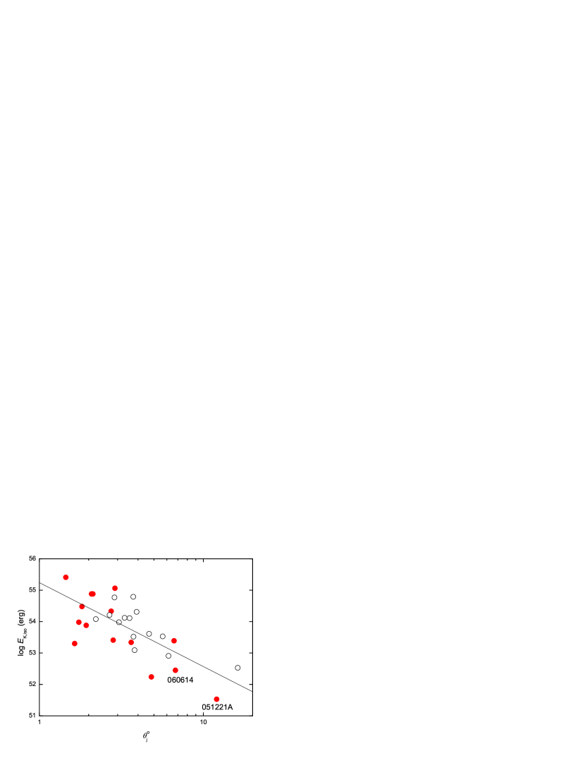
Figure 8: The $E_{\rm K,iso}$ as a function of $\theta_{j}$ for both the pre-Swift (open circles) and Swift GRBs (solid circles). The solid line is the best fit for both the pre-Swift and Swift GRBs.

The $\theta_{j}$ and $E_{K}$ distributions are shown in Fig.7. A sharp cutoff at $\theta_{j}\sim 1.5^{\rm o}$ is observed. The $\theta_{j}$ of the Swift GRBs derived from XRT observations tends to be smaller than that of the pre-Swift GRBs. The $E_{K}$ of the pre-Swift GRBs log-normally distribute around $1.5\times 10^{51}$ with a dispersion of 0.44 dex (at $1\sigma$ confidence level). However, the $E_{K}$ of the Swift GRBs randomly distribute in the range of $10^{50}\sim 10^{52}$ ergs (see also Kocevski & Butler 2007). We examine the correlation between $E_{\rm K,iso}$ and $\theta_{j}$ in Fig. 8. A tentative anti-correlation is found, but it has a large scatter. The best fit yields $E_{\rm K,iso}\propto\theta_{j}^{-2.35\pm 0.52}$, with a linear correlation coefficient $r=-0.66$ and a chance probability of $p\sim 10^{-4}$ (N=28). This suggests that although $E_{K}$ has a much larger scatter than the pre-Swift sample, it is still quasi-universal among bursts.

6 Conclusions and Discussion

We have presented a systematic analysis on the Swift/XRT data of 179 GRBs observed between Jan., 2005 and Jan., 2007 and the optical afterglow lightcurves of 57 GRBs detected before Jan. 2007, in order to systematically investigate the jet-like breaks in the X-ray and optical afterglow lightcurves. Among the 179 XRT lightcurves, 103 have good temporal coverage and have no significant flares in the afterglow phase. The 103 XRT lightcurves are fitted with the STPL, SBPL, or SPL model, and the spectral index of each segment of the lightcurves is derived by fitting the spectrum with a simple absorbed power law model. The same fitting is also made for the 57 optical light curves. We grade the jet break candidates through examining the data with the forward shock models with “Bronze”, “Silver”, “Gold”, or “Platinum”. We show that among the 103 well-sampled XRT lightcurves with a break, 42 are “Bronze”, and 27 are “Silver”. Twenty-seven out of 57 optical breaks are “Bronze”, and 23 “Silver”. Thirteen bursts have well-sampled lightcurves of both the X-ray and optical bands, but only 6 cases are consistent with being achromatic. Together with the GRB 990510 (in which an achromatic break in optical and radio bands can be claimed, Harrison et al. 1999), we have 7 “Gold” jet break candidates. However, none of them can be classified as “Platinum”, i.e. a textbook version of a jet break. Curiously, 7 out of the 13 jet-break candidates with multi-wavelength data suggest a chromatic break at the “jet break”, in contrary to the expectation of the jet models. The detection fraction of a jet break candidate in the XRT lightcurves is lower than that of the optical lightcurves, and the break time is also statistically earlier. These facts suggest that one should be very cautious in claiming a jet break and using the break information to infer GRB collimation and energetics.

On the other hand, the possibility that some of these breaks are jet breaks is not ruled out. The “Silver” and “Gold” jet break candidates have both the pre- and post-break temporal decay segments satisfying the simplest jet models, suggesting that these break are likely indeed jet breaks. In order to compare with the previous work on jet breaks, we then cautiously assume that the breaks in discussion are indeed jet breaks and proceed to constrain the $\theta_{j}$ and $E_{K}$ by using the X-ray afterglow data using the conventional jet models. We show that the geometrically corrected afterglow kinetic energy $E_{K}$ has a broader distribution than the pre-Swift sample, disfavoring the standard energy reservoir argument. On the other hand, a tentative anti-correlation between $\theta_{j}$ and $E_{\rm K,iso}$ is found for both the pre-Swift and Swift GRBs, indicating that the $E_{K}$ could still be quasi-universal.

The GRB jet models had been extensively studied in the pre-Swift era (e.g., Rhoads 1999; Sari et al. 1999; Panaitescu & Mészáros 1999; Moderski et al. 2000; Huang et al. 2000; Wei & Lu 2000; see reviews by Mészáros 2002; Zhang & Mészáros 2004; Piran 2005). The results of this paper suggest that for most bursts the X-ray and optical afterglows cannot be simultaneously explained within the simplest jet models. Data suggest that we may be missing some basic ingredients to understand GRB afterglows. There have been skepticism about the jet break interpretations before (e.g. Dai & Lu 1999; Wei & Lu 2002a,b). The current data call for more open-minded thoughts on the origin of lightcurve breaks (Zhang 2007). Observationally, at the epoch when the jet-like breaks show up the flux level is typically low. Source contaminations (e.g. GRB 060526; Dai et al. 2007) would complicate the picture. Careful analyses are needed to claim the breaks. On the other hand, most of the curious late afterglow break behaviors are likely not caused by these observational uncertainties. For example, even if the contamination source is removed, the broad band afterglow lightcurves of GRB 060526 (Dai et al. 2007) cannot be incorporated within any simplest jet models.

As cosmic beacons extending to high redshift universe (e.g. Lamb 2000; Bromm & Loeb 2002; Gou et al. 2004; Lin et al. 2004), GRBs have the potential to probe the high-$z$ universe. Using the pre-Swift jet break sample, Ghirlanda et al. (2004a) discovered a tight correlation between the cosmic rest-frame peak energy ($E_{p}$) of the GRB $\nu f_{\nu}$ spectrum and the geometrically-corrected GRB jet energy ($E_{\gamma}$). This correlation was taken as a potential standard candle to perform cosmography studies (e.g. Dai et al. 2004; Ghirlanda et al. 2004b). Liang & Zhang (2005) proceed with a model-independent approach, and derived a tight correlation among three observables, $E_{iso}$, $E_{p}^{{}^{\prime}}$, and $t^{{}^{\prime}}_{b,O}$, with the later being the cosmic rest frame optical break time only. This correlation was also used to constrain cosmological parameters (Liang & Zhang 2005; Wang & Dai 2006). As shown in this paper, it is difficult to accommodate both the X-ray and optical afterglow data within a unified jet model, so that the Ghirlanda relation is not longer supported by the Swift data. In fact, even with the optical data only, the Swift bursts make the Ghirlanda relation more dispersed than the pre-Swift sample (Campana et al. 2007). As shown in Figs. 4 and 6, the break times in the XRT lightcurves are significantly smaller than that in the optical lightcurves (most are pre-Swift bursts), but no significant difference is observed in the $E_{iso}$ distributions of the pre-Swift and Swift GRBs. These results tend to suggest that the jet break candidates in the XRT lightcurves do not share the same Liang-Zhang relation derived from the pre-Swift optical data. Since the energy band of Swift BAT is too narrow to reliably derive $E_{p}$ and $E_{iso}$ for most GRBs, it is non-trivial to test the Liang-Zhang relation rigorously. We plan to explore this interesting question in the future.

GRBs fall into short-hard and long-soft categories (Kouveliotou et al. 1993) or more generally Type I and Type II categories (Zhang et al. 2007b; Zhang 2006). The progenitors of the two classes are distinctly different: Type II GRBs are related to deaths of massive stars (Woosley & Bloom 2006 and references therein), and Type I GRBs are likely related to mergers of compact objects (Gehrels et al. 2005; Fox et al. 2005; Barthelmy et al. 2005; Berger et al. 2005a). Inspecting our sample of GRBs with known redshifts, there are two Type I GRBs: 051221A and 060614. Their X-ray afterglows are very bright, and the derived $E_{K}$ from the XRT data are $\sim 6\times 10^{49}$ ergs and $\sim 2\times 10^{50}$ ergs, respectively, roughly about 1 order of magnitude smaller than that of the typical Type II GRBs. The $\theta_{j}$ of the two bursts are $\sim 12^{\rm o}$ and $\sim 7^{\rm o}$, respectively. They are wider than those of the other (Type II) Swift GRBs in our sample. Combining our results with the fact that the $\theta_{j}$ of another short GRB 050724 is $>25^{\rm o}$ (Grupe et al.2006; Malesani et al. 2007), we cautiously suggest that the short GRBs might be less collimation, if the breaks are explained as a jet break.

Table 1: XRT observations and the Fitting results

GRB	$t_{1}$(ks)	$t_{2}$(ks)	$t_{b,1}(\delta t_{b,1})$(ks)	$t_{b,2}(\delta t_{b,2})$(ks)	$\alpha_{2}(\delta\alpha_{2})$	$\alpha_{3}(\delta\alpha_{3})$	$\alpha_{4}(\delta\alpha_{4}$)	$\chi^{2}$(dof)	$\Gamma_{2}(\delta\Gamma_{2})$	$\Gamma_{3}(\delta\Gamma_{3}$)	$\Gamma_{4}(\delta\Gamma_{4}$)
	STPL
050128	0.25	70.72	1.13(0.74)	30.67(14.19)	0.34(0.15)	1.00(0.13)	1.98(0.39)	27(46)	1.76(0.07)	2.05(0.08)	1.95(0.15)
060210	3.90	861.94	5.51(0.86)	186.65(76.48)	-0.20(0.39)	1.00(0.05)	1.85(0.27)	134(131)	–	2.12(0.08)	2.11(0.33)
060510A	0.16	343.41	2.89(1.87)	47.65(16.75)	0.01(0.09)	0.87(0.17)	1.74(0.12)	84(140)	1.91(0.07)	2.04(0.14)	2.06(0.14)
060807	0.28	166.22	3.80(1.15)	14.89(5.88)	-0.22(0.13)	0.96(0.24)	1.92(0.12)	42(34)	2.19(0.16)	2.18(0.09)	2.40(0.20)
060813	0.09	74.25	0.19(0.04)	15.24(3.88)	-0.01(0.19)	0.87(0.03)	1.63(0.13)	56(73)	2.05(0.09)	1.99(0.05)	2.10(0.07)
060814	0.87	203.31	5.92(2.88)	68.58(23.27)	0.32(0.13)	1.06(0.12)	2.38(0.40)	44(48)	2.21(0.05)	–	2.30(0.05)
	SBPL
050124	11.37	58.66	–	29.37(12.61)	–	0.62(0.56)	2.53(0.78)	6(11)	–	2.05(0.29)	1.93(0.21)
050315	5.40	450.87	–	224.64(38.68)	–	0.66(0.03)	1.90(0.28)	42(52)	–	2.31(0.12)	2.17(0.07)
050318	3.34	45.19	–	10.64(4.97)	–	0.90(0.23)	1.84(0.19)	27(20)	–	2.01(0.08)	2.02(0.06)
050319	6.11	84.79	11.20(13.26)	–	0.23(0.59)	0.99(0.25)	–	9(9)	2.00(0.06)	2.04(0.07)	–
050401	0.14	801.04	5.86(0.78)		0.58(0.02)	1.39(0.06)	–	107(92)	2.06(0.06)	2.03(0.04)	–
050416A	0.25	261.69	1.74(1.12)		0.43(0.12)	0.90(0.04)	–	36(38)	2.19(0.20)	2.15(0.10)	–
050505	3.07	97.19	7.87(1.57)		0.15(0.19)	1.30(0.06)	–	26(45)	2.00(0.07)	2.03(0.04)	–
050713A	4.61	1600.08	5.86(1.24)		-0.27(1.05)	1.16(0.03)	–	28(17)	2.25(0.05)	2.21(0.17)	–
050713B	0.79	478.50	10.80(1.59)		-0.00(0.07)	0.94(0.04)	–	40(63)	1.83(0.11)	1.94(0.09)	–
050716	0.64	74.40	7.53(9.02)		0.76(0.16)	1.35(0.24)	–	31(36)	1.60(0.08)	2.01(0.13)	–
050717	0.32	11.23	–	1.84(0.95)	–	0.57(0.21)	1.65(0.12)	28(56)	–	1.61(0.08)	1.89(0.12)
050726	0.42	17.05	–	1.17(0.33)	–	0.80(0.03)	2.32(0.22)	27(34)	–	2.06(0.08)	2.14(0.09)
050730	3.93	108.75	–	6.66(0.29)	–	-0.37(0.25)	2.49(0.04)	203(215)	–	1.65(0.03)	1.70(0.03)
050801	0.07	46.10	0.25(fixed)		0(fixed)	1.10(0.03)	–	44(45)	–	1.91(0.12)	–
050802	0.51	83.83	–	4.09(0.61)	–	0.32(0.10)	1.61(0.04)	58(72)	–	1.92(0.05)	1.89(0.07)
050803	0.50	368.89	–	13.71(0.90)	–	0.25(0.03)	2.01(0.07)	94(57)	–	1.78(0.10)	2.00(0.08)
050820A	4.92	1510.14	–	420.78(179.33)	–	1.11(0.02)	1.68(0.21)	246(292)	–	1.63(0.05)	1.87(0.04)
050822	6.41	523.32	66.99(44.38)		0.60(0.10)	1.25(0.19)	–	29(44)	2.29(0.23)	2.36(0.11)	–
050824	6.31	330.49	11.52(4.25)		-0.40(0.52)	0.61(0.06)	–	45(41)	2.00(0.16)	2.01(0.09)	–
050908	3.97	33.36	–	7.81(5.33)	–	0.13(0.96)	1.58(0.46)	0(1)	–	-	2.09(0.25)
050915A	0.32	88.77	1.94(1.11)		0.39(0.27)	1.24(0.09)	–	7(6)	2.32(0.17)	2.42(0.20)	–
051006	0.23	13.13		0.93(0.71)	–	0.57(0.26)	2.23(0.56)	15(19)	–	1.61(0.14)	1.84(0.20)
051008	3.09	43.77	14.67(3.82)		–	0.86(0.09)	2.01(0.19)	52(49)	–	2.15(0.32)	2.11(0.10)
051016A	0.37	37.41	0.63(0.40)		-0.41(1.18)	0.91(0.12)	–	0(7)	2.40(0.26)	–	–
051016B	4.78	150.47	–	66.40(23.09)	–	0.71(0.08)	1.84(0.46)	15(16)	–	-	2.19(0.13)
051109A	3.73	639.16	–	27.28(7.90)	–	0.79(0.07)	1.53(0.08)	39(48)	–	1.91(0.07)	1.90(0.07)
051109B	0.39	87.63	5.11(4.73)		0.56(0.17)	1.22(0.17)	–	15(17)	2.73(0.44)	2.35(0.24)	–
051117A	18.19	970.14	104.23(151.17)		0.51(0.25)	1.07(0.24)	–	21(19)	2.25(0.04)	2.39(0.15)	–
051221A	6.87	118.64	–	40.74(15.89)	–	0.46(0.16)	1.75(0.41)	11(14)	–	2.08(0.09)	2.02(0.19)
060105	0.10	360.83	–	2.31(0.14)	–	0.84(0.01)	1.72(0.02)	653(754)	–	2.23(0.05)	2.15(0.03)
060108	0.77	165.26	–	22.08(7.38)	–	0.26(0.09)	1.43(0.17)	7(7)	–	2.17(0.32)	1.75(0.15)
060109	0.74	48.01	4.89(1.10)		-0.17(0.14)	1.32(0.09)	–	19(13)	2.32(0.15)	2.34(0.14)	–
060124	13.30	664.01	–	52.65(10.33)	–	0.78(0.10)	1.65(0.05)	165(132)	–	2.10(0.06)	2.06(0.08)
060202	1.03	96.23	3.50(6.95)		0.68(0.37)	1.14(0.13)	–	51(31)	2.96(0.19)	3.41(0.14)	–
060203	3.80	32.95	–	12.95(6.69)	–	0.40(0.30)	1.65(0.47)	4(7)	–	2.08(0.19)	2.25(0.13)
060204B	4.06	98.80	–	5.55(0.66)	–	-0.49(0.65)	1.47(0.07)	21(34)	–	2.54(0.14)	2.64(0.16)
060206	0.11	621.77	8.06(1.46)		0.40(0.05)	1.26(0.04)	–	43(44)	2.31(0.12)	2.33(0.32)	–
060211A	5.40	527.10	–	267.24(165.67)	–	0.38(0.08)	1.63(1.27)	10(9)	–	2.15(0.06)	2.11(0.26)
060306	0.25	124.39	4.67(2.91)		0.40(0.11)	1.05(0.07)	–	30(32)	2.10(0.11)	2.21(0.10)	–
060313	0.09	93.22	–	11.18(2.89)	–	0.82(0.03)	1.76(0.18)	95(128)	–	1.84(0.34)	1.78(0.09)
060319	0.33	304.52	–	99.70(26.78)	–	0.84(0.02)	1.92(0.30)	72(93)	–	1.93(0.22)	2.25(0.11)
060323	0.33	16.28	–	1.29(0.32)	–	-0.11(0.23)	1.55(0.16)	4(7)	–	1.99(0.16)	2.02(0.13)
060428A	0.23	271.10	–	125.31(47.19)	–	0.48(0.03)	1.46(0.37)	26(21)	–	2.11(0.24)	1.97(0.10)
060428B	0.96	200.36	3.95(5.55)		0.53(0.41)	1.16(0.13)	–	19(21)	2.41(0.24)	2.10(0.33)	–
060502A	0.24	593.06	–	72.57(15.05)	–	0.53(0.03)	1.68(0.15)	11(26)	–	2.11(0.29)	2.15(0.13)
060507	3.00	86.09	6.95(1.68)		-0.06(0.55)	1.12(0.07)		– 13(24)	2.06(0.23)	2.15(0.14)	–
060510B	4.40	77.71	–	67.90(29.88)	–	0.44(0.18)	2.40(0.00)	4(8)	–	1.71(0.04)	–
060526	1.09	45.20	–	11.60(6.39)	–	0.42(0.12)	1.58(0.34)	5(9)	–	2.07(0.09)	2.08(0.16)
060604	4.14	403.81	11.51(9.81)		0.20(0.77)	1.17(0.09)	–	32(36)	2.44(0.15)	2.43(0.17)	–
060605	0.25	39.85	–	7.14(0.93)	–	0.45(0.04)	1.80(0.13)	22(34)	–	1.62(0.17)	1.83(0.09)
060614	5.03	451.71	–	49.84(3.62)	–	0.18(0.06)	1.90(0.07)	70(54)	–	2.02(0.02)	1.93(0.06)
060707	5.32	813.53	22.21(54.08)		0.37(0.96)	1.09(0.17)	–	8(11)	1.88(0.08)	2.06(0.20)	–
060708	0.25	439.09	7.28(2.34)		0.57(0.08)	1.32(0.07)	–	39(35)	2.30(0.20)	2.36(0.11)	–
060712	0.56	317.56	7.89(2.67)		0.12(0.16)	1.15(0.10)	–	15(14)	3.21(0.38)	2.94(0.28)	–
060714	0.32	331.97	3.70(0.97)		0.34(0.10)	1.27(0.05)	–	53(73)	2.15(0.08)	2.04(0.11)	–
060719	0.28	182.15	9.57(2.70)		0.40(0.06)	1.31(0.10)	–	19(26)	2.35(0.13)	2.28(0.26)	–
060729	0.42	2221.24	72.97(3.02)		0.21(0.01)	1.42(0.02)	–	459(459)	2.33(0.08)	2.29(0.07)	–
060804	0.18	122.07	0.86(0.22)		-0.09(0.15)	1.12(0.07)	–	18(24)	2.04(0.23)	2.14(0.15)	–
060805A	0.23	75.91	1.30(0.70)		-0.17(0.41)	0.97(0.13)	–	11(17)	–	1.97(0.37)	–
060906	1.32	36.69	–	13.66(3.29)	–	0.35(0.10)	1.97(0.36)	3(7)	–	2.28(0.37)	2.12(0.17)
060908	0.08	363.07	–	0.95(0.34)	–	0.70(0.07)	1.49(0.09)	98(59)	–	2.01(0.22)	2.00(0.08)
060912	0.12	86.80	2.92(2.77)		0.65(0.12)	1.24(0.11)	–	31(56)	–	2.03(0.12)	–
060923A	0.22	280.62	3.33(1.03)		-0.16(0.22)	1.30(0.06)	–	34(21)	2.05(0.25)	1.86(0.18)	–
060923B	0.16	6.03	0.42(0.64)		-0.73(0.99)	1.08(0.82)	–	2(10)	2.47(0.53)	2.25(0.31)	–
060926	0.09	5.96	1.13(0.92)		0.04(0.14)	1.23(0.52)	–	11(9)	1.93(0.16)	1.88(0.14)	–
060927	0.11	5.64	–	4.24(8.22)	–	0.73(0.32)	1.82(2.60)	4(7)	–	1.65(0.19)	1.92(0.15)
061004	0.39	69.99	1.50(0.52)		-0.08(0.29)	1.04(0.09)	–	13(17)	1.84(0.34)	3.04(0.34)	–
061019	9.07	287.03	10.84(2.15)		-1.38(2.88)	1.15(0.08)	–	6(10)	2.32(0.20)	1.93(0.28)	–
061021	0.30	594.16	9.59(2.17)		0.52(0.03)	1.08(0.03)	–	94(87)	1.90(0.06)	1.72(0.05)	–
061121	4.89	353.10	–	24.32(4.38)	–	0.75(0.06)	1.63(0.05)	121(147)	–	1.71(0.03)	1.96(0.07)
061201	0.10	15.42	–	2.09(0.75)	–	0.57(0.07)	1.61(0.23)	20(29)	–	1.30(0.09)	–
061222A	10.94	724.64	–	60.51(8.89)	–	0.81(0.07)	1.86(0.06)	144(95)	–	2.45(0.06)	2.22(0.12)
070103	0.11	143.98	–	2.88(0.48)	–	0.20(0.10)	1.63(0.08)	43(30)	–	2.32(0.25)	2.52(0.21)
070129	1.32	546.36	20.12(3.14)		0.15(0.07)	1.31(0.06)	–	42(70)	2.25(0.07)	2.30(0.10)	–
	SPL
050219B	3.21	85.26			–	1.14(0.03)	–	24(32)	–	2.27(0.14)	–
050326	3.34	142.24			–	–	1.63(0.04)	45(34)	–	–	2.15(0.14)
050408	2.60	3223.36			–	0.78(0.01)	–	52(44)	–	2.01(0.18)	–
050525A	5.94	157.85			–	1.40(0.05)	–	11(11)	–	2.17(0.18)	–
050603	39.72	166.22			–	–	1.71(0.10)	8(10)	–	–	1.84(0.09)
050721	0.30	257.24			–	1.18(0.02)	–	80(98)	–	1.77(0.10)	–
050814	2.17	87.85			–	0.65(0.05)	–	21(16)	–	1.91(0.07)	–
050826	0.13	61.93			–	1.02(0.03)	–	23(21)	–	2.19(0.19)	–
050827	65.95	246.35			–	1.24(0.15)	–	12(15)	–	1.88(0.15)	–
051001	6.71	273.86			–	0.70(0.06)	–	30(25)	–	1.93(0.19)	–
051111	10.98	34.24			–	1.09(0.17)	–	1(6)	–	–	–
051117B	0.22	0.62			–	–	1.68(0.27)	0(2)	–	–	–
060115	5.44	326.04			–	0.88(0.04)	–	12(12)	–	2.50(0.38)	–
060116	0.21	6.87			–	0.88(0.06)	–	3(6)	–	2.33(0.39)	–
060403	0.05	79.82			–	–	1.67(0.07)	70(57)	–	–	1.58(0.13)
060418	0.20	201.65			–	1.45(0.02)	–	272(283)	–	2.24(0.05)	–
060421	0.12	6.52			–	0.93(0.05)	–	11(7)	–	1.60(0.35)	–
060512	0.11	104.01			–	1.39(0.02)	–	76(58)	–	3.60(0.19)	–
060522	5.50	432.75			–	1.07(0.10)	–	7(13)	–	–	–
060825	0.23	63.15			–	1.08(0.04)	–	4(6)	–	1.64(0.29)	–
061007	0.09	97.82			–		1.68(0.01)	2153(1880)	–	–	2.08(0.05)
061019	2.90	287.03			–	0.95(0.03)	–	28(20)	–	2.12(0.21)	–
070110	43.70	439.51			–	1.05(0.14)	–	9(5)	–	2.36(0.24)	–

Table 2: Optical Data and the Fitting results

GRB	$t_{1}$(ks)	$t_{2}$(ks)	$t_{b,O}(\delta t_{b,O})$(ks)	$\alpha_{O,3}(\delta\alpha_{O,3})$	$\alpha_{O,4}(\delta\alpha_{O,4})$	$\chi^{2}$(dof)
970508	30.00	7421.93	139.67(3.16)	-2.73	1.21(0.02)	29(21)
980703	81.26	343.92	214.92(10.15)	1.11	2.83	7(7)
990123	13.31	1907.45	155.13(78.79)	0.98(0.10)	1.71(0.10)	12(8)
990510	12.44	340.24	101.91(12.48)	0.86(0.03)	1.95(0.14)	17(17)
990712	15.25	2991.47	2000.00(fixed)	0.97	2.32	15(11)
991216	41.17	1100.60	248.71(67.63)	1.22(0.04)	2.17	27(13)
000301	134.00	4198.10	562.87(18.70)	1.04	2.97	25(24)
000926	74.48	591.61	175.18(4.62)	1.48	2.49	35(24)
010222	13.09	2124.75	32.12(3.62)	0.43(0.08)	1.29(0.02)	29(48)
011211	34.40	2755.47	198.66(16.68)	0.85(0.05)	2.36	26(33)
020124	5.77	2787.67	8.47(7.39)	0.76(1.19)	1.85(0.11)	8(9)
020405	85.04	882.60	236.88(15.90)	1.21	2.48	6(10)
020813	14.18	362.83	40.03(0.21)	0.63	1.42	69(43)
021004	21.12	2030.14	300.30(fixed)	0.82(0.02)	1.39(0.05)	82(90)
030226	17.34	609.12	88.83(16.30)	0.88(0.12)	2.41(0.12)	10(12)
030323	34.68	895.74	400.00(fixed)	1.29	2.11	10(10)
030328	4.90	227.46	18.50(4.32)	0.52(0.09)	1.25(0.05)	52(70)
030329	4.60	100.00	41.00(0.42)	0.84	1.89(0.01)	870(956)
030429	12.53	574.04	158.73(fixed)	0.72(0.03)	2.72	30(10)
030723	15.00	800.00	103.22(5.02)	0.05(0.06)	2.01(0.05)	20(15)
040924	0.95	134.12	1.49(0.96)	0.34(0.64)	1.11(0.06)	19(10)
041006	0.23	550.00	14.24(1.15)	0.44(0.02)	1.27(0.01)	97(69)
050319	0.03	3.00	0.61(0.25)	0.38(0.06)	1.02(0.12)	29(29)
050525	2.83	91.80	40.72(8.18)	1.02(0.12)	3.00(0.57)	28(5)
050730	0.07	358.90	11.61(1.95)	0.26(0.08)	1.67(0.09)	58(16)
050801	0.02	9.49	0.20(0.01)	0.00(0.02)	1.11(0.01)	140(42)
050820A	0.12	663.30	344.98(32.78)	0.88(0.01)	1.48	439(25)
050922C	0.25	69.60	3.13(2.75)	0.63(0.13)	1.14(0.10)	14(17)
051109A	0.04	265.20	36.02(8.28)	0.68(0.01)	1.42(0.12)	116(40)
051111	0.03	20.00	2.61(0.25)	0.79(0.01)	1.70(0.14)	107(84)
060206	20.00	201.58	71.21(3.65)	1.07(0.02)	1.96	25(50)
060210	0.09	7.19	0.72(0.17)	0.04(0.22)	1.21(0.05)	13(12)
060526	0.06	893.55	84.45(5.88)	0.67(0.02)	1.80(0.04)	116(56)
060605A	0.43	111.96	8.83(1.21)	0.41	2.33(0.16)	2(1)
060607A	0.07	13.73	0.16(fixed)	-3.07(0.25)	1.18(0.02)	92(35)
060614	20.00	934.36	112.35(8.53)	0.77(0.10)	2.70(0.07)	16(16)
060714	3.86	285.87	10.00(fixed)	0.01	1.41(0.03)	35(11)
060729	70.00	662.39	297.49(69.62)	1.09(0.10)	2.13(0.44)	18(19)
061121	0.26	334.65	1.70(0.73)	0.17	0.99(0.05)	18(23)
980326	36.46	117.68		2.14(0.09)		15(6)
991208	179.52	613.24	-	2.30(0.12)		17(9)
000131	357.44	699.06	-	2.55(0.29)	-	0(1)
000418	214.27	2000.00	-	0.81(0.03)	-	13(9)
000911	123.35	1466.26	-	1.36(0.06)	-	9(2)
011121	33.36	1000.00	-	1.98(0.06)	-	7(5)
021211	0.13	1865.64	-	1.18(0.01)	-	78(50)
050318	3.23	22.83	-	0.84(0.22)	-	0(1)
050401	0.06	1231.18	-	0.80(0.01)	-	43(12)
050408	8.64	434.81	-	0.72(0.04)	-	9(15)
050502	6.12	29.22	-	1.42(0.02)	-	31(19)
050603	34.09	219.71	-	1.75(0.20)	-	16(7)
050802	0.34	127.68	-	0.85(0.02)	-	50(10)
050908	1.32	57.81	-	0.71(0.09)	-	11(10)
060124	3.34	1979.30	-	0.85(0.02)	-	11(19)
060418	3.92	69.53	-	1.36(0.04)	-	8(11)
060904B	0.50	163.13	-	0.86(0.02)	-	60(19)
070110	0.66	34.76	-	0.43(0.08)	-	1(4)

Table 3: Definition of Jet Break Candidate Grades

Grade	No Spectral Evolution	$\alpha_{4}>1.5$	Closure Relations	Achromaticity	Number
“Bronze”	Y	Y			42(XRT)+27(Opt.)
“Silver”	Y	Y	Y		27(XRT)+23(Opt.)
“Gold”	Y	Y	Y(1 band)	Y	7
“Platinum”	Y	Y	Y (at least 2 bands)	Y	0

Table 4: Jet Break Candidates and Their Grades

GRB	$\beta_{2}(\delta\beta_{2})$	$\beta_{4}(\delta\beta_{4})$	$\alpha_{3}(\delta\alpha_{3})$	$\alpha_{4}(\delta\alpha_{4})$	$t_{j}(\delta t_{j})$(ks)	$\Delta\alpha(\delta\Delta\alpha)$	Grade	Achromaticity
Radio
970508					$\sim 25$ (days)		Bronze	?
000418					$\sim 26$ (days)		Bronze	?
Optical
980703	1.01(0.02)	–	1.11	2.83	214.92(10.15)	1.71	Silver	?
990123	0.80(0.10)	–	0.98(0.10)	1.71(0.10)	155.13(78.79)	0.73(0.14)	Silver	?
990510	0.75(0.07)	–	0.86(0.03)	1.95(0.14)	101.91(12.48)	1.09(0.14)	Gold	$\surd$
990712	0.99(0.02)	–	0.97	2.32	2000	1.35	Silver	?
991216	0.74(0.05)	–	1.22(0.04)	2.17	248.71(67.63)	0.95(0.04)	Silver	?
000301C	0.90(0.02)	–	1.04	2.82	562.87(18.70)	1.78	Silver	?
000926	1.00(0.20)	–	1.48	2.49	175.18(4.62)	1.01	Silver	?
011211	0.74(0.05)	–	0.85(0.05)	2.36	198.66(16.68)	1.52(0.05)	Silver	?
020124	0.91(0.14)	–	0.76(1.19)	1.85(0.11)	8.47(7.39)	1.09(1.19)	Silver	?
020405	1.23(0.12)	–	1.21	2.48	236.88(15.90)	1.27	Silver	?
020813	0.85(0.07)	–	0.63	1.42	40.03(0.21)	0.79	Silver	?
021004	0.39(0.12)	–	0.65(0.02)	1.57(0.05)	300.30	0.92(0.05)	Silver	?
030226	0.70(0.03)	–	0.88(0.12)	2.41(0.12)	88.83(16.30)	1.53(0.17)	Silver	?
030323	0.89(0.04)	–	1.29	2.11	400	0.82	Silver	?
030329	0.66	–	0.84	1.89(0.01)	41.00(0.42)	1.05(0.01)	Gold	$\surd$
030429	1.22(0.04)	–	0.72(0.03)	2.72	158.73	2.00(0.03)	Silver	?
030723	1	–	0.05(0.06)	2.01(0.05)	103.22(5.02)	1.96(0.08)	Bronze	?
050525	0.97(0.10)	–	1.02(0.12)	3.00(0.57)	40.72(8.18)	1.98(0.58)	Gold	$\surd$
050730	0.75	–	0.26(0.08)	3.00(0.57)	1.67(0.09)	2.74(0.58)	Bronze	?
050820A	0.57(0.06)	–	0.88(0.01)	1.48	344.98(32.78)	0.60	Gold	$\surd$
051109A	0.65(0.15)	–	0.68(0.01)	1.42(0.12)	36.02(8.28)	0.74(0.12)	Gold	$\surd$
051111	0.84(0.02)	–	0.79(0.01)	1.70(0.14)	2.61(0.25)	0.91(0.14)	Silver	X
060206	0.70	–	1.07(0.02)	2.00(0.26)	71.21(3.65)	0.93(0.26)	Silver	X
060605	0.8	–	0.41	2.33(0.16)	8.83(1.21)	1.92	Bronze	$\surd$
060526	1.69(0.53)	–	0.67(0.02)	1.80(0.04)	84.45(5.88)	1.13(0.04)	Gold	$\surd$
060614	0.94(0.08)	–	0.77(0.10)	2.70(0.07)	112.35(8.53)	1.93(0.12)	Gold	$\surd$
060729	0.74(0.07)	–	1.09(0.10)	2.13(0.44)	297.49(69.62)	1.03(0.45)	Silver	X
X-Ray
980828	$\sim 1$		1.44	2.6	190	1.16	Silver	?
030329	1.17	0.8(0.3)	0.87(0.05)	1.84(0.07)	44.93(4.32)	0.97(0.09)	Gold	$\surd$
050124	1.05(0.29)	0.93(0.21)	0.62(0.56)	2.53(0.78)	29.37(12.61)	1.91(0.96)	Silver	?
050128	1.05(0.08)	0.95(0.15)	1.00(0.13)	1.98(0.39)	30.70(14.20)	0.98(0.41)	Silver	?
050315	1.31(0.12)	1.17(0.07)	0.66(0.03)	1.90(0.23)	224.64(38.68)	1.24(0.23)	Silver	?
050318	1.01(0.08)	1.02(0.06)	0.90(0.23)	1.84(0.19)	10.60(4.97)	0.94(0.30)	Silver	X
050525A	1.17(0.18)	1.17(0.18)	1.20(0.03)	1.62(0.16)	13.73(7.47)	0.42(0.16)	Gold	$\surd$
050717	0.61(0.08)	0.89(0.12)	0.57(0.21)	1.65(0.12)	1.84(0.95)	1.08(0.24)	Silver	?
050726	1.06(0.08)	1.14(0.09)	0.79(0.03)	2.32(0.22)	8.78(1.11)	1.53(0.22)	Silver	?
050730	0.65(0.03)	0.70(0.03)	-0.37(0.25)	2.49(0.04)	6.66(0.29)	2.86(0.25)	Bronze	$\surd$
050802	0.92(0.05)	0.89(0.07)	0.32(0.10)	1.61(0.04)	4.09(0.61)	1.29(0.11)	Bronze	X
050803	0.78(0.10)	1.00(0.08)	0.25(0.03)	2.01(0.07)	13.71(0.90)	1.76(0.08)	Bronze	?
050820A	0.63(0.05)	0.87(0.04)	1.11(0.02)	1.68(0.21)	421.00(179.00)	0.57(0.21)	Gold	$\surd$
050908	2.09(0.25)	1.09(0.25)	0.13(0.96)	1.58(0.46)	7.81(5.33)	1.45(1.06)	Bronze	X
051006	0.61(0.14)	0.84(0.20)	0.57(0.26)	2.23(0.56)	0.93(0.71)	1.66(0.62)	Silver	?
051008	1.15(0.32)	1.11(0.10)	0.86(0.09)	2.01(0.19)	14.67(3.82)	1.15(0.21)	Silver	?
051016B	1.19(0.13)	1.19(0.13)	0.71(0.08)	1.84(0.46)	66.40(23.09)	1.13(0.47)	Silver	?
051109A	0.91(0.07)	0.90(0.07)	0.79(0.07)	1.53(0.08)	27.28(7.90)	0.74(0.11)	Gold	$\surd$
051221A	1.07(0.36)	1.02(0.19)	1.20(0.06)	1.92(0.52)	354.00(103.00)	0.72(0.52)	Silver	$\surd$
060105	1.23(0.05)	1.15(0.03)	0.84(0.01)	1.72(0.02)	2.31(0.14)	0.88(0.02)	Silver	?
060108	1.17(0.32)	0.75(0.15)	0.26(0.09)	1.43(0.17)	22.08(7.38)	1.17(0.19)	Bronze	?
060124	1.10(0.06)	1.06(0.08)	0.81(0.09)	1.66(0.05)	52.60(10.30)	0.85(0.10)	Silver	X
060203	1.08(0.19)	1.25(0.13)	0.40(0.30)	1.65(0.47)	12.95(6.69)	1.25(0.56)	Bronze	?
060204B	1.54(0.14)	1.64(0.16)	-0.49(0.65)	1.47(0.07)	5.55(0.66)	1.96(0.65)	Bronze	?
060210	1.12(0.08)	1.11(0.33)	1.00(0.05)	1.85(0.27)	187.00(76.50)	0.85(0.27)	Silver	X
060211A	1.15(0.06)	1.11(0.26)	0.38(0.08)	1.63(1.27)	267.24(165.67)	1.25(1.27)	Bronze	?
060313	0.84(0.34)	0.78(0.09)	0.82(0.03)	1.76(0.18)	11.18(2.89)	0.94(0.18)	Silver	?
060319	0.93(0.22)	1.25(0.11)	0.84(0.02)	1.92(0.30)	99.70(26.78)	1.08(0.30)	Silver	?
060323	0.99(0.16)	1.02(0.13)	-0.11(0.23)	1.55(0.16)	1.29(0.32)	1.66(0.28)	Bronze	?
060428A	1.11(0.24)	0.97(0.10)	0.48(0.03)	1.46(0.37)	125.31(47.19)	0.98(0.37)	Bronze	?
060502A	1.11(0.29)	1.15(0.13)	0.53(0.03)	1.68(0.15)	72.57(15.05)	1.15(0.15)	Bronze	?
060510A	1.04(0.05)	1.06(0.14)	0.93(0.14)	1.77(0.10)	47.70(16.70)	0.84(0.17)	Silver	?
060526	1.07(0.09)	1.08(0.16)	0.42(0.12)	1.58(0.34)	11.60(6.39)	1.16(0.36)	Gold	$\surd$
060605	0.62(0.17)	0.83(0.09)	0.45(0.04)	1.80(0.13)	7.14(0.93)	1.35(0.14)	Bronze	$\surd$
060614	0.96(0.16)	0.93(0.06)	1.03(0.02)	2.13(0.07)	36.60(2.40)	1.10(0.07)	Gold	$\surd$
060807	1.18(0.09)	1.40(0.20)	0.96(0.24)	1.92(0.12)	14.90(5.88)	0.96(0.27)	Silver	?
060813	0.99(0.05)	1.10(0.07)	0.87(0.03)	1.63(0.13)	15.20(3.88)	0.76(0.13)	Silver	?
060814	1.30(0.05)	1.30(0.05)	1.06(0.12)	2.38(0.40)	68.60(23.30)	1.32(0.42)	Silver	?
060906	1.28(0.37)	1.12(0.17)	0.35(0.10)	1.97(0.36)	13.66(3.29)	1.62(0.37)	Bronze	?
060908	1.01(0.22)	1.00(0.08)	0.70(0.07)	1.49(0.09)	0.95(0.34)	0.79(0.11)	Bronze	?
060927	0.65(0.19)	0.92(0.15)	0.73(0.32)	1.82(2.60)	4.24(8.22)	1.09(2.62)	Silver	?
061121	0.71(0.03)	0.96(0.07)	0.75(0.06)	1.63(0.05)	24.32(4.38)	0.88(0.08)	Silver	?
061201	0.30(0.15)	0.30(0.15)	0.57(0.07)	1.61(0.23)	2.09(0.75)	1.04(0.24)	Bronze	?
061222A	1.45(0.06)	1.22(0.12)	0.81(0.07)	1.86(0.06)	60.50(8.89)	1.05(0.09)	Silver	?
070103	1.32(0.25)	1.52(0.21)	0.20(0.10)	1.63(0.08)	2.88(0.48)	1.43(0.13)	Bronze	?

References. — a:Frail et al.(2000); b:Berger et al.(2001);c: Blustin et al. (2006); d: Burrows et al. (2006); e: Dai et al. (2007); f: Mangano et al. (2007)

Table 5: Derivation of Jet Opening Angles and Kinetic Energies

GRB	$z$	Reg.	$p$	$\epsilon_{B,-4}$	$Y$	$\theta_{j}(^{o})$	$\log E_{\rm K,iso}$	$\log E_{\rm K}$	$\log\nu_{m}$	$\log\nu_{c}$	ref.
050315	1.95	I	2.76	1.00	2.45	2.9	55.06	52.17(0.05)	11.71	16.61	1
050318	1.44	I	2.08	1.01	6.91	1.6	53.30	49.91(0.16)	11.86	18.00	2
050319	3.24	I	2.16	1.00	4.93	$>$2.5	53.76	$>$50.75	11.69	17.70	3
050401	2.9	II	2.98	0.20	2.59	$>$4.2	54.97	$>$52.40	12.51	$>$18.00	4
050416A	0.65	I	2.32	10.78	0.72	$>$9.3	51.94	$>$50.06	11.80	$>$18.00	5
050505	4.27	I	2.1	1.00	6.28	$>$2.5	54.03	$>$51.00	11.56	17.53	6
050525A	0.606	II	3.34	0.99	0.10	2.6	53.98	50.99(0.06)	12.79	$>$18.69	7
050820A	2.61	I	2.01	1.00	11.05	3.6	54.88	52.17(0.14)	9.65	17.08	8
050922C	2.2	II	2.44	1.49	3.16	$>$2.9	53.24	$>$50.35	13.15	$>$18.00	9
051016B	0.94	I	2.18	3.30	1.31	4.82	52.24	49.79(0.12)	10.31	18.00	10
051221A	0.5465	I	2.14	9.76	0.79	12.06	51.53	49.87(0.10)	10.19	18	11
060124	2.3	II	3.12	0.23	1.06	1.5	55.41	51.91(0.06)	12.11	$>$18.00	12
060206	4.05	I	2.62	1.00	2.65	1.8	54.48	51.18(0.02)	11.74	16.90	13
060210	3.91	I	2.24	1.00	5.75	2.7	54.33	51.39(0.14)	12.25	17.37	14
060502A	1.51	II	3.3	0.79	0.15	2.1	54.88	51.71(0.07)	12.04	18.00	15
060512	0.44	II	3.36	1.00	0.12	$>$6.1	52.38	$>$50.14	13.41	$>$19.09	16
060522	5.11	I	2.26	1.00	2.91	$>$4.8	53.17	$>$50.73	11.50	17.81	17
060526	3.21	I	2.14	1.01	5.26	2.82	53.41	50.49(0.02)	11.58	17.65	18
060604	2.68	I	2.54	1.00	2.38	$>$4.6	53.75	$>$51.26	12.02	17.59	19
060605	3.7	II	2.98	0.60	2.38	$>$1.6	54.21	$>$50.81	13.32	$>$18.00	20
060614	0.13	II	2.72	1.00	0.43	6.8	52.45	50.30(0.02)	10.74	$>$18.32	21
060714	2.71	I	2.12	1.00	4.26	$>$5.1	53.32	$>$50.91	11.17	17.94	22
060729	0.54	I	2.26	1.00	2.42	6.6	53.39	51.21(0.08)	9.93	17.54	23
060814	0.84	I	2.60	2.33	1.41	3.63	53.34	50.64(0.12)	12.6	18 0	24
060908	2.43	II	2.5	1.00	1.62	$>$8.4	52.78	$>$50.81	11.99	$>$18.26	25
060912	0.94	I	2.01	1.02	7.06	$>$4.4	52.88	$>$50.35	9.46	17.98	26
060926	3.2	I	2.01	1.01	15.71	$>$0.9	54.21	$>$50.26	11.21	17.21	27
061007	1.26	II	3.16	1.00	1.93	$>$7.6	53.99	$>$51.94	14.35	$>$18.22	28
061121	1.31	II	2.7	0.95	1.01	1.93	53.88	50.63(0.06)	11.57	18.01	29
070110	2.35	I	2.72	1.00	1.70	$>$7.8	54.31	$>$52.27	11.38	16.98	30

References. — 1: Kelson & Berger(2005); 2: Berger & Mulchaey(2005); 3: Fynbo et al.(2005a); 4: Fynbo et al.(2005b); 5: Cenko et al.(2005; 6: Berger et al.(2005c); 7: Fynbo et al.(2005c); 8: Ledoux et al.(2005); 9: D’Elia et al.(2005); 10: Soderberg et al.(2005); 11: Berger & Soderberg(2005); 12: Cenko et al.(2006a); 13: Aoki et al.(2006); 14: Cucchiara et al.(2006a); 15: Cucchiara et al.(2006b); 16: Bloom et al.(2006a); 17: Cenko et al.(2006b); 18: Berger & Gladders(2006); 19: Castro-Tirado et al.(2006); 20: Still et al.(2006); 21: Fugazza et al.(2006); 22: Jakobsson et al.(2006a); 23: Thoene et al.(2006) ; 24:Thoene (2007); 25:Rol et al.(2006); 26: Jakobsson et al.(2006b); 27: D’Elia et al.(2006); 28: Jakobsson et al.(2006c); 29: Bloom et al.(2006b); 30: Jaunsen et al.(2006)

Table 6: Observations of pre-Swift GRBs derived parameters

GRB	$z$	Reg.	time (s)	$F_{x}(\delta F_{X}$)	$\alpha(\delta\alpha)$	$\beta$	$t_{j}$(ks)	$\theta^{o}$	$\theta_{j}$ (rad)	$p$	$\epsilon_{B,-4}$	$Y$	$E_{\rm K,iso}$	$E_{\rm K}$	$\log\nu_{m}$	$\log\nu_{c}$
970508	0.835	I	47160	7.13	1.1	$1.14^{+0.51}_{-0.36}$	2160.00(432.00)	16.7	0.391	2.28	3.4	1.34	52.53	51.15(0.07)	11.26	18.00
970828	0.958	II	14400	118	1.44(0.07)	$1.1^{+0.3}_{-0.3}$	190.08(34.56)	3.9	0.128	3.2	0.99	0.80	54.31	51.68(0.06)	13.46	18.20
980703	0.966	I	122400	4(1)	1.24(0.18)	$1.77^{+0.6}_{{}_{0}.47}$	214.92(10.15)	6.1	0.2	2.1	1.01	3.52	52.91	50.67(0.02)	9.81	17.87
990123	1.6	I	84240	19.11(2.2)	1.41(0.05)	$0.99^{0.07}_{-0.08}$	155.13(787.86)	2.9	0.089	2.98	0.40	1.51	54.77	51.87(0.18)	12.32	18.00
990510	1.619	I	42120	32.8(1.4)	1.41(0.18)	$1.19^{+0.14}_{-0.14}$	101.91(124.81)	3.1	0.054	2.38	1.00	3.63	53.98	51.14(0.04)	12.07	17.62
990705	0.84	II	52200	1.9(0.6)	–	1.05	86.40(17.28)	3.8	0.096	3.1	0.99	0.22	53.52	50.85(0.06)	12.18	18.67
991216	1.02	II	39240	250(10)	1.61(0.07)	$0.7^{+0.1}_{-0.1}$	248.71(67.63)	3.7	0.051	2.01	1.0	11/11	54.79	52.12(0.11)	9.57	17.29
000926	2.307	I	197640	2.23(0.77)	–	$0.9^{+0.3}_{-0.2}$	175.18(4.62)	3.3	0.14	2.01	1.00	7.11	54.12	51.34(0.01)	8.29	17.16
010222	1.477	I	117720	1.87(0.18)	1.33(0.04)	$1^{+0.1}_{-0.1}$	80.35(12.96)	2.7	0.08	2.02	1.00	7.59	54.21	51.25(0.05)	9.21	17.29
011211	2.14	II	29600	0.248	0.95(0.02)	$1.16^{+0.03}_{0.03}$	198.66(16.68)	3.5	-	3.32	0.99	0.21	54.11	51.39(0.02)	12.84	18.31
020405	0.689	I	147600	13.6(2.5)	1.15(0.95)	$1^{+0.2}_{-0.1}$	236.88(15.90)	5.7	0.285	2.02	1.00	5.55	53.53	51.21(0.02)	8.63	17.67
020813	1.254	II	114840	22	1.42(0.05)	$0.8^{+0.1}_{-0.1}$	397.44(0.864)	2.2	0.066	2.6	0.55	1.86	54.08	50.95(0.01)	11.57	18.00
021004	2.323	I	113040	4.3(0.7)	1(0.2)	$1.1^{+0.1}_{-0.1}$	300.30(8.64)	4.7	0.24	2.2	1.00	3.69	53.61	51.13(0.01)	10.85	17.54
030329	0.1678	I	22377	157.0(8.7)	1.2(0.1)	$1.17\pm 0.04$	40.95(0.43)	3.8	0.052	2.34	2.15	2.23	53.09	50.43(0.01)	11.95	18.00

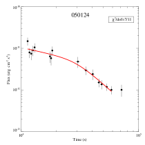
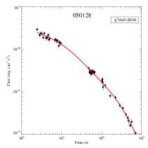
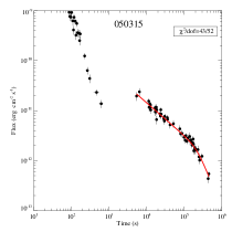
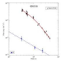
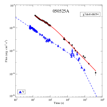
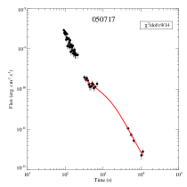
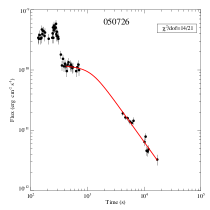
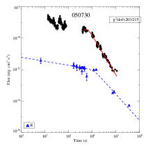
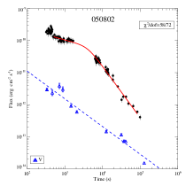
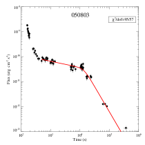
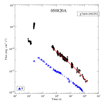
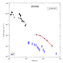
Figure 2: The X-ray (solid dots) and optical (open triangles) lightcurves and their fitting results as well for derived the jet break candidates .

Fig.2— continued.

Fig.2— continued

Fig.2— continued

Fig.2— continued

Fig. 2— continued

Figure 5: Comparison of the $\theta_{j}$ derived from the X-ray afterglow with that from the prompt gamma-ray emission (from Frail et al. 2001). The line is $\theta_{j}=\theta_{j}^{{}^{\prime}}$.

References

- Aoki et al. (2006) Aoki, K., Hattori, T.,Kawabata, K. S., & Kawai, N. 2006, GCN, 4703, 1
- Barthelmy et al. (2005) Barthelmy, S. D., et al. 2005, Nature, 438, 994
- Berger & Gladders (2006) Berger, E., & Gladders, M. 2006, GCN, 5170, 1
- Berger & Mulchaey (2005) Berger, E., & Mulchaey, J. 2005, GCN, 3122, 1
- Berger & Soderberg (2005) Berger, E., & Soderberg, A. M. 2005, GCN, 4384, 1
- Berger et al. (2001) Berger, E., et al. 2001, ApJ, 556, 556
- Berger et al. (2003) Berger, E., Kulkarni, S. R., & Frail, D. A. 2003, ApJ, 590, 379
- Berger et al. (2005a) Berger, E. et al. 2005a, Nature, 438, 988
- Berger et al. (2005b) Berger, E. et al. 2005b, ApJ, 634, 501
- Berger et al. (2005c) Berger, E., Cenko, S. B., Steidel, C., Reddy, N., & Fox, D. B. 2005c, GCN, 3368, 1
- Bloom et al. (2003) Bloom, J. S., Frail, D. A., & Kulkarni, S. R. 2003, ApJ, 594, 674
- Bloom et al. (2006a) Bloom, J. S., Foley,R. J., Koceveki, D., & Perley, D. 2006a, GCN, 5217, 1
- Bloom et al. (2006b) Bloom, J. S., Perley,D. A., & Chen, H. W. 2006b, GCN, 5826, 1
- Blustin et al. (2006) Blustin, A. J., et al. 2006, ApJ, 637, 901
- Bromm & Loeb (2002) Bromm, V., & Loeb, A. 2002, ApJ, 575, 111
- Burrows & Racusin (2007) Burrows, D. N., & Racusin, J. 2007, preprint(astro-ph/200702633)
- Burrows et al. (2005a) Burrows, D. N., et al. 2005a, Space Science Reviews, 120, 165
- (18) Burrows, D. N., et al. 2005b, Science, 309, 1833
- Burrows et al. (2006) Burrows, D. N., et al. 2006, ApJ, 653, 468
- Campana et al. (2007) Campana, S., Guidorzi, C., Tagliaferri, G., Chincarini, G., Moretti, A., Rizzuto, D., & Romano, P. 2007, A&A, 472, 395
- Castro-Tirado et al. (2006) Castro-Tirado,A. J., Amado, P., Negueruela, I., Gorosabel, J., Jelinek, M., & de Ugarte Postigo, A. 2006, GCN, 5218, 1
- Cenko et al. (2005) Cenko, S. B., et al. 2005, GCN, 3542, 1
- Cenko et al. (2006a) Cenko, S. B., Berger, E., & Cohen, J. 2006a, GCN, 4592, 1
- Cenko et al. (2006b) Cenko, S. B., et al. 2006b, GCN, 5155, 1
- Chevalier & Li (2000) Chevalier, R. A., & Li, Z.-Y. 2000, ApJ, 536, 195
- Chincarini et al. (2007) Chincarini, G., et al. 2007, ApJ, submitted (arXiv:astro-ph/0702371)
- Covino et al. (2006) Covino, S., et al. 2006, arXiv:astro-ph/0612643
- Cucchiara et al. (2006a) Cucchiara, A., Fox, D. B., & Berger, E. 2006, GCN, 4729, 1
- Cucchiara et al. (2006b) Cucchiara, A., Price, P. A., Fox, D. B., Cenko, S. B., & Schmidt, B. P. 2006, GCN, 5052, 1
- Curran et al. (2007) Curran, P. A., et al. 2007, MNRAS, in press(arXiv:0706.1188)
- Dai & Cheng (2001) Dai, Z. G., & Cheng, K. S. 2001, ApJ, 558, L109
- Dai & Lu (1999) Dai, Z. G. & Lu, T. 1999, ApJ, 519, L155
- Dai & Lu (1998) Dai, Z. G., & Lu, T. 1998, A&A, 333, L87
- Dai et al. (2004) Dai, Z. G., Liang, E. W., & Xu, D. 2004, ApJ, 612, L101
- Dai et al. (2007) Dai, X., Halpern, J. P., Morgan, N. D., Armstrong, E., Mirabal, N., Haislip, J. B., Reichart, D. E., & Stanek, K. Z. 2007, ApJ, 658, 509
- D’Elia et al. (2005) D’Elia, V., et al. 2005, GCN, 4044, 1
- D’Elia et al. (2006) D’Elia, V., et al. 2006, GCN, 5637, 1
- Della Valle et al. (2006) Della Valle, M., et al. 2006, Nature, 444, 1050
- Djorgovski et al. (2001) Djorgovski, S. G., Frail, D. A., Kulkarni, S. R., Bloom, J. S., Odewahn, S. C., & Diercks, A. 2001, ApJ, 562, 654
- Falcone et al. (2007) Falcone, A. D., et al. 2007, ApJ, submitted (arXiv:0706.1564)
- Fox et al. (2005) Fox, D. B., et al. 2005, Nature, 437, 845
- Frail et al. (2000) Frail, D. A., Waxman, E., & Kulkarni, S. R. 2000, ApJ, 537, 191
- Frail et al. (2001) Frail, D. A., et al. 2001, ApJ, 562, L55
- Fugazza et al. (2006) Fugazza, D., et al. 2006, GCN, 5276, 1
- Fynbo et al. (2005a) Fynbo, J. P. U., Hjorth,J., Jensen, B. L., Jakobsson, P., Moller, P., & Naranen, J. 2005a, GCN, 3136, 1
- Fynbo et al. (2005b) Fynbo, J. P. U., et al. 2005b, GCN, 3176, 1
- Fynbo et al. (2005c) Fynbo, J. P. U., et al. 2005c, GCN, 3749, 1
- Fynbo et al. (2006) Fynbo, J. P. U., et al. 2006, Nature, 444, 1047
- Gal-Yam et al. (2006) Gal-Yam, A., et al. 2006, Nature, 444, 1053
- Gehrels et al. (2004) Gehrels, N., et al. 2004, ApJ, 611, 1005
- Gehrels et al. (2006) Gehrels, N., et al. 2006, Nature, 444, 1044
- Ghirlanda et al. (2004a) Ghirlanda, G., Ghisellini, G., Lazzati, D., & Firmani, C. 2004a, ApJ, 613, L13
- Ghirlanda et al. (2004b) Ghirlanda, G., Ghisellini, G., & Lazzati, D. 2004b, ApJ, 616, 331
- Gou et al. (2004) Gou, L. J., Mészáros, P., Abel, T., Zhang, B. 2002, ApJ, 604, 508
- Grupe et al. (2006) Grupe, D., Burrows, D. N., Patel, S. K., Kouveliotou, C., Zhang, B., Mészáros, P., Wijers, R. A. M., & Gehrels, N. 2006, ApJ, 653, 462
- Harrison et al. (1999) Harrison, F. A., et al. 1999, ApJ, 523, L121
- Huang, Gou, Dai, & Lu (2000) Huang, Y. F.,Gou, L. J., Dai, Z. G., & Lu, T. 2000, ApJ, 543, 90
- Ioka et al. (2005) Ioka, K., Kobayashi, S., & Zhang, B. 2005, ApJ, 631, 429
- Ioka et al. (2006) Ioka, K., Toma, K., Yamazaki, R., & Nakamura, T. 2006, A&A, 458, 7
- Jakobsson et al. (2006a) Jakobsson, P., et al. 2006a, A&A, 460, L13
- Jakobsson et al. (2006b) Jakobsson, P., Vreeswijk, P., Fynbo, J. P. U., Hjorth, J., Starling, R., Kann, D. A., & Hartmann, D. 2006a, GCN, 5320, 1
- Jakobsson et al. (2006c) Jakobsson, P., Levan, A., Chapman, R., Rol, E., Tanvir, N., Vreeswijk, P., & Watson, D. 2006b, GCN, 5617, 1
- Jakobsson et al. (2006e) Jakobsson, P., et al. 2006e, A&A, 447, 897
- Jaunsen et al. (2006) Jaunsen, A. 0., et al. 2006, GCN, 6010, 1
- Jin & Fan (2007) Jin, Z. P., & Fan, Y. Z. 2007, MNRAS, 378, 1043
- Kelson & Berger (2005) Kelson, D., & Berger, E. 2005, GCN, 3101, 1
- King et al. (2007) King, A., Olsson, E., & Davies, M. B. 2007, MNRAS, 374, L34
- Kobayashi & Zhang (2007) Kobayashi, S., & Zhang, B. 2007, ApJ, 655, 973
- Kocevski & Butler (2007) Kocevski, D., & Butler, N. 2007, arXiv:0707.4478
- Kouveliotou et al. (1993) Kouveliotou, C., Meegan, C. A., Fishman, G. J., Bhat, N. P., Briggs, M. S., Koshut, T. M., Paciesas, W. S., & Pendleton, G. N. 1993, ApJ, 413, L101
- Kumar & Panaitescu (2000) Kumar, P., & Panaitescu, A. 2000, ApJ, 541, L9
- Lamb (2000) Lamb, D. Q. 2000, Phys. Rep., 333, 505
- Ledoux et al. (2005) Ledoux, C., et al. 2005, GCN, 3860, 1
- Liang & Zhang (2005) Liang, E., & Zhang, B. 2005, ApJ, 633, 611
- Liang et al. (2004) Liang, E. W., Dai, Z. G., Wu, X. F. 2004, ApJ, 606, L29
- Liang et al. (2006) Liang, E. W., et al. 2006, ApJ, 646, 351
- Liang et al. (2007) Liang, E.-W., Zhang, B.-B., & Zhang, B. 2007, ApJ, in press(arXiv:0705.1373) (Paper II)
- Lin et al. (2004) Lin, J. R., Zhang, S. N., & Li, T. P. 2004, ApJ, 605, 819
- Malesani et al. (2007) Malesani, D., et al. 2007, A&A, 473, 77
- Mészáros (2006) Mészáros, P. 2006, Reports of Progress in Physics, 69, 2259
- Mészáros (2002) Mészáros, P. 2002, ARA&A, 40, 137
- Mangano et al. (2007) Mangano, V., et al. 2007, ArXiv e-prints, 704, arXiv:0704.2235
- Meszaros & Rees (1993) Mészáros, P., & Rees, M. J. 1993, ApJ, 405, 278
- Moderski et al. (2000) Moderski, R., Sikora, M., & Bulik, T. 2000, ApJ, 529, 151
- Molinari et al. (2007) Molinari, E., et al. 2007, A&A, 469, L13
- Mondardini et al. (2006) Monfardini, A. et al. 2006, ApJ, 648, 1125
- Nousek et al. (2006) Nousek, J. A., et al. 2006, ApJ, 642, 389
- O’Brien et al. (2006) O’Brien, P. T., et al. 2006a, ApJ, 647, 1213
- O’Brien et al. (2006) O’Brien, P. T., Willingale, R., Osborne, J. P., & Goad, M. R. 2006b, New Journal of Physics, 8, 121
- Panaitescu & Kumar (2002) Panaitescu, A., & Kumar, P. 2002, ApJ, 571, 779
- Panaitescu & Mészáros (1999) Panaitescu, A., & Mészáros, P. 1999, ApJ, 526, 707
- Panaitescu et al. (2006) Panaitescu, A., Mészáros, P., Burrows, D., Nousek, J., Gehrels, N., O’Brien, P., & Willingale, R. 2006, MNRAS, 369, 2059
- Panaitescu (2005) Panaitescu, A. 2005, MNRAS, 363, 1409
- Panaitescu (2007a) Panaitescu, A. 2007, MNRAS, 380, 374
- Piran (2005) Piran, T. 2005, Reviews of Modern Physics, 76, 1143
- Rhoads (1999) Rhoads, J. E. 1999, ApJ, 525,737
- Rol et al. (2006) Rol, E., Jakobsson, P., Tanvir, N., & Levan, A. 2006, GCN, 5555, 1
- Sako, Harrison, & Rutledge (2005) Sako, M., Harrison, F. A., & Rutledge, R. E. 2005, ApJ, 623, 973
- Sari et al. (1998) Sari, R., Piran, T., & Narayan, R. 1998, ApJ, 497, L17
- Sari et al. (1999) Sari, R., Piran, T., & Halpern, J. P. 1999, ApJ, 519, L17
- Sato et al. (2007) Sato, G., et al. 2007, ApJ, 657, 359
- Shen et al. (2006) Shen, R., Kumar, P., & Robinson, E. L. 2006, MNRAS, 371, 1441
- Soderberg et al. (2005) Soderberg, A. M., Berger, E., & Ofek, E. 2005, GCN, 4186, 1
- Still et al. (2006) Still, A., et al. 2006, GCN, 5226, 1
- Thoene et al. (2006) Thoene, C. C., et al. 2006, GCN, 5373, 1
- Thoene et al. (2007) Thoene, C. C., Perley, D. A. , & Bloom, J. S. 2007, GCN 6663
- Tominaga et al. (2007) Tominaga, N., et al. 2007, ApJ, 657, L77
- Troja et al. (2007) Troja, E., et al. 2007, ApJ, 665, 599
- Wang & Dai (2006) Wang, F. Y., & Dai, Z. G. 2006, MNRAS, 368, 371
- Wei & Lu (2000) Wei, D. M., & Lu, T. 2000, ApJ, 541, 203
- Wei & Lu (2002a) Wei, D. M., & Lu, T. 2002a, MNRAS, 332,994
- Wei & Lu (2002b) Wei, D. M. & Lu, T. 2002, A&A, 381, 731
- Wijers& Galama (1999) Wijers, R. A. M. J.& Galama, T. J. 1999, ApJ, 523, 177
- Willingale et al. (2004) Willingale, R., Osborne, J. P., O’Brien, P. T., Ward, M. J., Levan, A., & Page, K. L. 2004, MNRAS, 349, 31
- Willingale et al. (2007) Willingale, R., et al. 2007, ApJ, 662, 1093
- Woosley & Bloom (2006) Woosley, S. E., & Bloom, J. S. 2006, ARA&A, 44, 507
- Wu et al. (2004) Wu, X. F., Dai, Z. G., Liang, E. W. 2004, ApJ, 615, 359
- Yamazaki et al. (2006) Yamazaki, R., Toma, K., Ioka, K., & Nakamura, T. 2006, MNRAS, 369, 311
- Yost et al. (2003) Yost, S. A., Harrison, F. A., Sari, R., & Frail, D. A. 2003, ApJ, 597, 459
- Zhang (2006) Zhang, B. 2006, Nature, 444, 1010
- Zhang & Mészáros (2004) Zhang, B., & Mészáros, P. 2004, International Journal of Modern Physics A, 19, 2385
- Zhang (2007) Zhang, B. 2007, Chinese Journal of Astronomy and Astrophysics, 7, 1
- Zhang et al. (2004) Zhang, B., Dai, X., Lloyd-Ronning, N. M., & Mészáros, P. 2004, ApJ, 601, L119
- Zhang et al. (2006) Zhang, B., Fan, Y. Z., Dyks, J., Kobayashi, S., Mészáros, P., Burrows, D. N., Nousek, J. A., & Gehrels, N. 2006, ApJ, 642, 354
- (125) Zhang, B., et al. 2007a, ApJ, 655, 989
- (126) Zhang, B., Zhang, B.-B., Liang, E.-W., Gehrels, N., Burrows, D. N., & Mészáros, P. 2007b, ApJ, 655, L25
- Zhang et al. (2007c) Zhang, B.-B., Liang, E.-W., & Zhang, B. 2007c, ApJ, 666, 1002