The Rockefeller University, 1230 York Avenue, New York, NY 10021, USA.

()

We use the work done on and the heat removed from a system to maintain it in a nonequilibrium steady state for a thermodynamic-like description of such a system as well as of its fluctuations. Based on a generalized Onsager-Machlup theory for nonequilibrium steady states we indicate two ambiguities, not present in an equilibrium state, in defining such work and heat: one due to a non-uniqueness of time-reversal procedures and another due to multiple possibilities to separate heat into work and an energy difference in nonequilibrium steady states. As a consequence, for such systems, the work and heat satisfy multiple versions of the first and second laws of thermodynamics as well as of their fluctuation theorems. Unique laws and relations appear only to be obtainable for concretely defined systems, using physical arguments to choose the relevant physical quantities. This is illustrated on a number of systems, including a Brownian particle in an electric field, a driven torsion pendulum, electric circuits and an energy transfer driven by a temperature difference.

1 Introduction

Of all steady states of systems, the equilibrium state is by far the most studied. First, a thermodynamic description has been developed involving the work done by or on the system or the heat produced by or removed from the system. This leads to the first law of thermodynamics, i.e. the law of energy conservation, while the introduction of entropy leads to the second law of thermodynamics, i.e. that entropy changes in a closed system have to be non-negative.

A generalization to systems in nonequilibrium steady states (NESS) has been made as a special case of the general theory of thermodynamics of irreversible processes (irreversible thermodynamics) for systems in local, i.e. near equilibrium [1]. This theory has in turn been enlarged to an extended irreversible thermodynamics [2], where in addition to the usual local quantities (local mass density, local velocity and local energy density) also the corresponding irreversible thermodynamic currents of mass, momentum and energy (or heat) are taken into account for a description of the system. Also in that context NESSs can be considered. NESSs, as well as their fluctuations, have also be considered in hydrodynamics [3].

The major difference between all these thermodynamic theories of NESSs and the attempt proposed here to describe NESSs, is that all these theories are ultimately based on a direct generalization of equilibrium thermodynamics and, in particular, the use of the same concepts of work and heat as in equilibrium. To the contrary, the theory developed here introduces fundamentally different definitions of work and heat, associated with a NESS, rather than those used in the above equilibrium thermodynamic based theories. In fact, we propose a thermodynamic-like description of systems in NESSs by defining the work associated with such a system as the work that has to be done on the system to maintain it in its NESS and prevent it from decaying to an equilibrium state. Similarly we define the heat associated with such a system as the heat that has to be removed from the system to eliminate the heat produced by the irreversible (nonequilibrium) processes which take place in such systems.

We develop this theory for NESS using a generalization of the classical path integral theory of Onsager and Machlup [4] for fluctuations in the equilibrium state to NESSs, used already by us in two previous papers for a specific model [5, 6]. An introduction to this theory, relevant for this paper, can be found in the first paper [5]. The present paper attempts to present the general structure, applied to a variety of models, for discussing the NESS as a generalization of the equilibrium state and to exhibit the conceptual differences between these two steady states of a system and their fluctuations.

In fact, contrary to the NESS, the equilibrium state is an absolutely stable state, which maintains itself without the necessity of any work to be done on it, nor of the removal of any spontaneously produced heat, since this heat vanishes on average in an equilibrium state. For that reason the Onsager-Machlup theory of fluctuations of the equilibrium state, does not consider any work done on the system and only considers the entropy production rate associated with the fluctuations in the equilibrium state. The absence of any work allows the formulation of a theory of fluctuations in the equilibrium state, based on the entropy production associated with these fluctuations, alone. Therefore the Onsager-Machlup theory does not contain any equilibrium thermodynamic feature.

This is completely different for a NESS, where the presence of external “forces” (characterized by appropriate nonequilibrium parameters), keeps the system permanently out of equilibrium, requiring “actions” involving work and heat to maintain this system in a NESS and prevent it from decaying to the absolutely stable equilibrium state. Then a generalization of the two laws of equilibrium thermodynamics is possible, which require, however, NESS adapted definitions of work and heat, which are, together with the internal energy, the ingredients of a thermodynamic-like formulation of the NESS.

The generalization of the Onsager-Machlup theory for fluctuations in the equilibrium state to one for NESS, turned out to be non-trivial. This, since such a generalization involves in general ambiguities, i.e. multiple a priori possible choices for the work, heat and energy and their fluctuations in a NESS. The Onsager-Machlup theory for the equilibrium state provides us though with a starting point to deal with these problems and to obtain a physically unique description of the thermodynamic laws and the fluctuations of a NESS, at least for the specific models considered in this paper.

Implementation of the above outlined program is based on Onsager and Machlup’s path integral method. This involves, not only the above mentioned new definitions of the NESS adapted thermodynamic-like quantities of work and heat, but also new definitions of forward and corresponding backward paths in time because of the presence of external nonequilibrium parameters in the NESS. The main difficulty and the origin of these ambiguities arising then is that an appropriate choice of a backward path for a given forward path is not unique and depends on the nature of the system in the NESS. In addition, there is an intrinsic ambiguity because work and energy differences can only be defined up to a common quantity. It appears at present that these ambiguities can only be resolved on physical grounds for specific concrete models.

The contents of this paper are organized in three parts as follows. After the introduction in this section 1, we introduce in Sec. 2 the class of systems in NESSs which we will consider in this paper. We studied three classes. (A) Systems under a constant force, such as an electrically charged Brownian particle in a fluid subject to an external electric field $\mathcal{E}$ [cf. Fig. 1(a)]; (B) Systems coupled to an oscillator, as, e.g. a Brownian particle confined by a harmonic oscillator, which is dragged through the fluid with a constant velocity $v$ by an outside force [cf. Fig. 2(a)]; (C) Systems with two random noise sources. An example is two independent heat reservoirs at different temperatures, each containing a Brownian particle, which are coupled to each other harmonically, allowing an energy current from one reservoir to the other [cf. Fig. 3(a)]. For each class we introduce not only Brownian particle models but also corresponding electric circuit models. In total we consider eight models: two of Class A, four of Class B and two of Class C. Each of these models can be described by a Langevin equation, which is given explicitly in a common form in the next section 3 by Eq. (17).

In the second part of the paper, in Sec. 3, we discuss the generalized Onsager-Machlup theory for a NESS and show how to obtain appropriate definitions of the heat and work from our general point of view. We first introduce the path integral method for the Langevin dynamics (17), based on a Lagrangian to give a probability functional of paths. Then, following Onsager and Machlup, we write this Lagrangian for the NESS as a sum of two dissipation functions and an entropy production rate, where the latter allows us a definition of the heat in the NESS by integrating over time and multiplying by the temperature of a heat reservoir, connected to the system. By minimizing this Lagrangian we obtain the average path, which then leads to the non-negativity of the entropy production for the average path, i.e. the validity of the second law of thermodynamics for the average path. Finally, using the energy conservation law (the first law of thermodynamics), the work is obtained as a sum of the heat and the internal energy difference. This work consists of four parts: (i) work given by the partial time-derivative of the internal energy, (ii) work done by an external driving force, (iii) work caused by a time-irreversible force, and (iv) work by a temperature difference between reservoirs.

In this part of the paper we also discuss in detail the role of time-reversal for our NESS Onsager-Machlup theory. We point out in detail the difficulties associated with the ambiguity of defining an appropriate backward path associated with a given forward path due to the presence of external nonequilibrium parameters $\bf\mu$, e.g. a dragging velocity $v$ or an electric field $\mathcal{E}$, which specify the NESS forces or currents. To formulate this ambiguity, a time-reversal operator $\hat{I}_{\pm}$ is introduced which reverses (indicated by a hat) the direction of the (internal) motion (the velocity) of the system, as compared with that on the forward path, as well as a possible, but not necessary, reversal of the sign of the external nonequilibrium parameter $\bf\mu$ (indicated by $\pm$ in $\hat{I}_{\pm}$). Two possible definitions can therefore be given for the heat, corresponding to a $+$ or $-$ sign in $\hat{I}_{\pm}$, respectively, as well as for the work and the internal energy, leading to two possible expressions for the energy conservation law, or the first law as well as for the second law of (NESS) thermodynamics for each (not only the average) path.

In Sec. 4 we discuss the nonequilibrium detailed balance relations and the transient fluctuation theorems [10] for work, which hold for both $\hat{I}_{+}$ and $\hat{I}_{-}$. All the above laws and relations are therefore unaffected by the ambiguities mentioned above, i.e. they are valid relations for the NESS, independent of the above ambiguities. For the transient fluctuation theorems this must be due to the fact that they are mathematical identities [11]. This means here that one obtains two formal identities, without the need to identify the appropriate thermodynamic work on physical grounds, as is necessary for a physical discussion of particular systems. This “universal” validity of the transient fluctuation theorems could disappear for asymptotic fluctuation theorems [12] for NESSs as was indeed shown in a previous paper for the case of a dragged Brownian particle model [5].

In the third part of the paper, Sec. 5, we will illustrate how the above mentioned ambiguities can be eliminated and lead to unique choices of the heat and work to maintain a NESS on a variety of models introduced in Sec. 2. Although these models are all linear we do not expect the nature of our considerations to be qualitatively changed, if non-linearities in the potentials, occurring in these models, are introduced. However, the dependence of, in particular, fluctuations on the properties of the stochastic noise is much less clear [13, 14].

2 NESS Models

Before discussing our generalized Onsager-Machlup theory for NESSs, we introduce some typical NESS models all described by Langevin equations. Using these models, we give concrete examples of external nonequilibrium parameters which specify the system in a NESS (so are zero at equilibrium) and change their signs with a reversal of the steady state force or current. These parameters play a crucial role in this paper and co-determine the choice of the proper time reversal procedure to calculate relevant work and heat to associate with a system, as will be discussed later. The internal energies for these models are also given in this section and will be used to determine the work to maintain a NESS in the following sections. As mentioned in Sec. 1, we discuss these NESS models by separating them into three classes: Class A for models driven by a constant external force, Class B for systems coupled to an oscillator, and Class C for models with two random noises.

2.1 Class A: Systems under a Constant Force

a) The first (and possibly simplest) example is an electrically charged Brownian particle in a fluid in a uniform electric field. The Langevin equation for this system is given by

$$m\ddot{x}_{s}=q\mathcal{E}-\alpha\dot{x}_{s}+\zeta_{s}$$ (1)

for the particle position $x_{s}$ at the time $s$, where $m$ is the mass, $q$ the electric charge of the particle, $\mathcal{E}$ a constant external electric field, $\alpha$ the friction coefficient of the particle in the fluid, $\ddot{x}_{s}\equiv d^{2}x_{s}/ds^{2}$ and $\dot{x}_{s}\equiv dx_{s}/ds$. Here, $\zeta_{s}$ is a Gaussian-white random force whose first two auto-correlations are given by $\langle\zeta_{t}\rangle=0$ and $\langle\zeta_{t_{1}}\zeta_{t_{2}}\rangle=(2\alpha/\beta)\delta(t_{1}-t_{2})$, respectively, with $\beta$ the inverse temperature of the heat reservoir and the notation $\langle\cdots\rangle$ for an ensemble average. The Brownian particle is driven by a constant force $q\mathcal{E}$ via the external field $\mathcal{E}$ which plays the role of the external nonequilibrium parameter in this model and vanishes at equilibrium. A schematic illustration for this system is given in Fig. 1(a). The internal energy $E$ of this system is given by

$$E(\dot{x}_{s})=\frac{1}{2}m\dot{x}_{s}^{2}.$$ (2)

It is important to note that here we regards $q\mathcal{E}$ as an “external” driving force and its corresponding potential energy is not included in the “internal” energy $E$. In this system, the Brownian particle achieves a constant average velocity $\overline{v}=q\mathcal{E}/\alpha$ in a NESS. Note that a nonequilibrium state driven by a constant force can be realized in variety of other ways, for example, in a Brownian particle under a constant gravitational force.

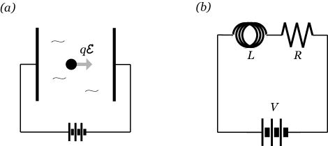
Figure 1: NESS models of Class A: (a) a charged particle driven by a constant electric field and (b) an electric circuit consisting of an inductor and resistor in series. For an explanation of the symbols, see the text.

b) As a second example we consider an electric circuit consisting of an inductor (with self-inductance $L$) and a resistor (with resistance $R$) in series [15], as shown in Fig. 1(b). In this circuit, the voltage $V$ of the battery is equal to $L\dot{I}_{s}+RI_{s}+\delta V_{s}$ with the electric current $I_{s}$ through the resistor and a voltage random noise $\delta V_{s}$ in the resistor. Combining this with $I_{s}=\dot{q}_{s}$, where $q_{s}$ is the charge in the resistor, we obtain the Langevin equation

$$L\ddot{q}_{s}=V-R\dot{q}_{s}-\delta V_{s}.$$ (3)

Here, we assume that $\delta V_{s}$ is a Gaussian-white random noise whose first two auto-correlations are given by $\langle\delta V_{s}\rangle=0$ and $\langle\delta V_{s}\delta V_{s^{\prime}}\rangle=(2R/\beta)\delta(s-s^{\prime})$ by the Johnson-Nyquist theorem [16, 17]. The external nonequilibrium parameter in this model is given by the voltage $V$ of the battery. We note that the two Langevin equations (1) and (3) have the same form. We summarized correspondences of the quantities in these two equations in Table 1. Noting these correspondences, the energy $E$ of this electric circuit model is given by Eq. (2) with a replacement of $m$ and $x_{s}$ by $L$ and $q_{s}$, respectively, i.e. by $E(\dot{q}_{s})=(1/2)L\dot{q}_{s}^{2}$.

Model					Class A	Class B
Brownian particle	$x_{s}$	$m$	$\alpha$	$\zeta_{s}$	$q\mathcal{E}$	$\kappa$ $v$
Electric circuit	$q_{s}$	$L$	$R$	$-\delta V_{s}$	V	$1/C$ $I$ (parallel) $CA$ (serial)
Torsion pendulum	$\theta_{s}$	$\mathcal{I}$	$\nu$	$\zeta_{s}$		$\sigma$ $\xi/\sigma$

Table 1: Correspondences of quantities in various NESS models. The external nonequilibrium parameters characterizing the deviations of the systems from an equilibrium state are $\mathcal{E}$ and $V$ in Class A, and $v$, $I$, $A$ and $\xi$ in Class B, respectively. Explanation of symbols is in the text.

2.2 Class B: Systems coupled to a Harmonic Oscillator

As the second class of NESS models, we consider a system under an oscillating force.

a) The first example in this class is a Brownian particle confined by a harmonic potential which is dragged by a constant velocity $v$ in a fluid [5, 6, 18, 19]. The Langevin equation for this system is given by

$$m\ddot{x}_{s}=-\kappa(x_{s}-vs)-\alpha\dot{x}_{s}+\zeta_{s}$$ (4)

for the particle position $x_{s}$ with the oscillator spring constant $\kappa$ and the Gaussian-white random force $\zeta_{s}$. In this model, the dragging velocity $v$ plays the role of the external nonequilibrium parameter which is zero at equilibrium. A schematic illustration of this model is given in Fig. 2(a). In this model the internal energy $E$ of the particle is given by

$$E(\dot{x}_{s},x_{s})=\frac{1}{2}m\dot{x}_{s}^{2}+\frac{1}{2}\kappa(x_{s}-vs)^{2}$$ (5)

where the second term on its right-hand side is the potential energy of the particle in the harmonic oscillator.

Although the model described by Eq. (4) may be regarded as a Brownian particle model producing a constant average velocity of the particle, like the electric field driven model described by Eq. (1), we should notice there are clear differences between these two models. In this dragged Brownian particle model (Class B), the particle moves with a constant velocity even if there is no friction, since the average velocity of the particle is independent of the friction constant $\alpha$. On the other hand, in the electric field driven model (Class A), the average velocity of the particle will depend on the friction constant and if there is no friction then the particle accelerates indefinitely. We also note that there is no explicit time-dependent parameter in the force in the electric field driven model, while in a Brownian particle dragged by a constant velocity there is an explicit time-dependence in the force via $vs$ in Eq. (4). These “simple” differences will manifest themselves in different definitions of work and heat in NESSs, as will be discussed in Secs. 5.1 and 5.2.

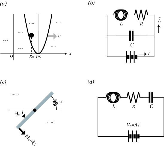
Figure 2: NESS models of Class B: (a) a particle dragged by a harmonic potential with a constant velocity, (b) an electric circuit with a serial inductor-resistor coupled to a capacitor in parallel, (c) a torsion pendulum confined by a spring with an external torque, and (d) an electric circuit with an inductor, resistor and capacitor in series. Symbols are defined in the test.

b) The same form as the Langevin equation (4) appears for an electric circuit in which an inductor and resistor in series are coupled with a capacitor in parallel [20], as shown in Fig. 2(b). We first derive a Langevin equation for this system. Denoting the electric current through the resistor by $\tilde{I}_{s}=\dot{q}_{s}$ with $q_{s}$ the charge through the resistance, as shown in Fig. 2(b), the voltage difference $V_{1s}$ between the ends of the inductor and resistor in series with the Johnson-Nyquist voltage fluctuation $\delta V_{s}$ as a Gaussian-white noise is given by $V_{1s}=L\dot{\tilde{I}\;}_{s}+R\tilde{I}_{s}+\delta V_{s}$. On the other hand, the voltage $V_{2s}$ applied to the capacitor (with the capacitance $C$) is given by $V_{2s}=(Is-q_{s})/C$ where $I$ is the constant electric current from the battery, as shown in Fig. 2(b). Here, we used that the charge of the capacitor is given by $Is-q_{s}$, i.e. the charge $Is$ received from the battery minus the charge $q_{s}$ taken to the resistor. Using that $V_{1s}=V_{2s}$ and $\tilde{I}_{s}=\dot{q}_{s}$ we obtain

$$L\ddot{q}_{s}=-\frac{1}{C}(q_{s}-Is)-R\dot{q}_{s}-\delta V_{s},$$ (6)

which is the Langevin equation for the charge $q_{s}$. The external nonequilibrium parameter of this system is given by $I$. Note that, different from the previous electric circuit model in Class A [cf. Eq. (3)] in which the voltage of the battery is constant, in this electric circuit model, described by Eq. (6), the electric current $I$ from the battery is assumed to be constant. The energy of this system is given by Eq. (5) with a replacement of $m$, $x_{s}$, $\kappa$, and $v$ by $L$, $q_{s}$, $1/C$ and $I$, respectively (cf. Table 1).

c) The third example of Class B is a torsion pendulum under an external torque in a fluid [21]. A schematic illustration of this model is given in Fig. 2(c) as a rod with the total moment of inertia $\mathcal{I}$, rotating around its center with a spring functioning as a torsion. The time-derivative $\mathcal{I}\ddot{\theta}_{s}$ of the angular momentum $\mathcal{I}\dot{\theta}_{s}$ for an angular displacement $\theta_{s}$ must be equal to the torque applied to the rod, so that the equation of motion for $\theta_{s}$ is given by the Langevin equation

$$\mathcal{I}\ddot{\theta}_{s}=-\sigma\theta_{s}+\mathcal{M}_{s}-\nu\dot{\theta}_{s}+\zeta_{s}$$ (7)

where $\nu$ is the viscous damping, $\sigma$ the elastic torsional stiffness of the pendulum, and $\mathcal{M}_{s}$ the external torque. For this model, we consider the case of a linear external torque of

$$\mathcal{M}_{s}=\xi s$$ (8)

with a force constant $\xi$. Since the pendulum is driven externally by the torque (8), its coefficient $\xi$ plays the role of the external nonequilibrium parameter. In this model the internal energy $E$ of the particle is given by

$$E(\dot{\theta}_{s},\theta_{s})=\frac{1}{2}\mathcal{I}\dot{\theta}_{s}^{2}+\frac{1}{2}\sigma\theta_{s}^{2}.$$ (9)

as the sum of the kinetic energy and the torsion energy.

It is important to note that although the Lagrangian equation (7) with the torque (8) has the same form as Eq. (4) (cf. Table 1), the energy (9) in this driven torsion pendulum model does not have the same form as the energy (5) for the dragged Brownian particle model. As shown later in this paper, this difference of energy also appears as a difference in the definition of the work. Another difference between these two models is that for the driven torsion pendulum model the average internal energy increases with time in a NESS, leading to a time-proportional work rate as will be discussed in Sec. 5.2, while in the dragged Brownian particle model the average internal energy is independent of time in a NESS with a constant average work rate.

d) As the last example in Class B, we consider an electric circuit consisting of an inductor, resistor and capacitor in series with a time-dependent applied voltage $V_{s}=As$ with a constant $A$ [20]. [See Fig. 2(d) for a schematic illustration of this model.] The Langevin equation for the charge $q_{s}$ is given by

$$L\ddot{q}_{s}=-\frac{q_{s}}{C}+As-R\dot{q}_{s}-\delta V_{s}.$$ (10)

In this model, the equilibrium state is realized when $A=0$, so that $A$ is the external nonequilibrium parameter. Note that the Langevin equation (10) has the same form as Eqs. (4), (6) and (7) (cf. Table 1). The energy of this system is given by Eq. (9) with the replacements of $m$, $x_{s}$ and $\kappa$ by $L$, $q_{s}$ and $1/C$, respectively (cf. Table 1).

2.3 Class C: Systems with Two Random Noises

As the last category of NESS models discussed in this paper, we introduce stochastic models with two random noises.

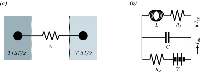
Figure 3: NESS models of Class C: (a) two harmonically coupled particles connected to two heat reservoirs with different temperatures, and (b) an electric circuit with two resistors.

a) The first example in this category consists of two Brownian particles coupled by a spring, where each particle is confined to a heat reservoir at a different temperature (cf. Refs. [19, 22]). We give a schematic illustration of this model in Fig. 3(a). The Langevin equation for the positions $x_{1s}$ and $x_{2s}$ of the first and second particle, respectively, is given by

$$m\ddot{x}_{js}=-\kappa\left(x_{js}-x_{ks}\right)-\alpha\dot{x}_{js}+\zeta_{js}$$ (11)

with $j\neq k$, $j=1,2$ and $k=1,2$. Here, $\zeta_{1s}$ and $\zeta_{2s}$ are two independent Gaussian-white random forces at different temperatures $T+\Delta T/2$ and $T-\Delta T/2$, respectively, so that $\langle\zeta_{js}\rangle=0$ and $\langle\zeta_{js}\zeta_{j^{\prime}s^{\prime}}\rangle=(2\alpha/\beta_{j})\delta_{jj^{\prime}}\delta(s-s^{\prime})$ with the inverse temperatures $\beta_{j}\equiv\{k_{B}[T+(-1)^{j+1}\Delta T/2]\}^{-1}$. For simplicity we assumed identical masses and friction coefficients for the two particles. In this system, a NESS is sustained with an energy transfer between the two reservoirs due to the temperature difference $\Delta T$ as an external nonequilibrium parameter. The internal energy $E$ of this system is given by

$$E(\dot{\mathbf{x}}_{s},\mathbf{x}_{s})=\sum_{j=1}^{2}\frac{1}{2}m\dot{x}_{js}^{2}+\frac{1}{2}\kappa\left(x_{1s}-x_{2s}\right)^{2}$$ (12)

with $\mathbf{x}_{s}\equiv(x_{1s},x_{2s})$.

b) We can consider a similar stochastic system with two random noises in an electric circuit as in Fig. 3(b), which is like that in Fig. 2(b), except for an additional resistance next to the battery. We denote by $I_{1s}=\dot{q}_{1s}$ the electric current associated with charge $q_{1s}$ through the resistor $1$ (with resistance $R_{1}$) next to the coil and by $I_{2s}=\dot{q}_{2s}$ the electric current associated with charge $q_{2s}$ through the resistor $2$ (with resistance $R_{2}$) next to the battery. The charge on the capacitor is given by $q_{2s}-q_{1s}$, so that the voltage drop in the capacitor is $(q_{2s}-q_{1s})/C$. This voltage drop is equal to the voltage difference $L\dot{I}_{1s}+R_{1}I_{1s}+\delta V_{1s}$ between the ends of the inductor and the resistor $1$ in series, and also to the one $V-R_{2}I_{2s}-\delta V_{2s}$ between the ends of the battery and the resistor $2$. Here, $\delta V_{1s}$ and $\delta V_{2s}$ are independent Gaussian-white random noises in the resistors $1$ and $2$, respectively, with $\langle\delta V_{js}\rangle=0$ and $\langle\delta V_{js}\delta V_{j^{\prime}s^{\prime}}\rangle=(2R_{j}/\beta)\delta_{jj^{\prime}}\delta(s-s^{\prime})$, $j=1,2$ and $j^{\prime}=1,2$. Using these voltages, the Langevin equation for the charges $q_{js}$ is given by

$$L\ddot{q}_{1s}+R_{1}\dot{q}_{1s}+\delta V_{1s}=V-R_{2}\dot{q}_{2s}-\delta V_{2s}=\frac{q_{2s}-q_{1s}}{C}.$$ (13)

In this system the electric current is driven by the voltage $V$, which is the external nonequilibrium parameter. The energy $E$ of this system is given by

$$E(\dot{\mathbf{q}}_{s},\mathbf{q}_{s})=\frac{1}{2}L\dot{q}_{1s}^{2}+\frac{\left(q_{1s}-q_{2s}\right)^{2}}{2C}$$ (14)

with $\mathbf{q}_{s}\equiv(q_{1s},q_{2s})$.

Although we categorize the above two models as a single class C, the corresponding Langevin equations (11) and (13) do not have exactly the same form, different from the models in Class A or B. However, we can introduce a single Langevin equation, which reduces to Eqs. (11) and (13) as special cases:

$$m_{j}\ddot{x}_{js} = \Gamma\delta_{j2}-\kappa\left(x_{js}-x_{ks}\right)-\alpha_{j}\dot{x}_{js}+\zeta_{js},$$ (15)

with $j\neq k$, $j=1,2$ and $k=1,2$, a constant $\Gamma$ and two independent Gaussian-white random noises $\zeta_{1s}$ and $\zeta_{2s}$ at different temperatures $T+\Delta T/2$ and $T-\Delta T/2$, respectively, so that $\langle\zeta_{js}\rangle=0$ and $\langle\zeta_{js}\zeta_{j^{\prime}s^{\prime}}\rangle=(2\alpha_{j}/\beta_{j})\delta_{jj^{\prime}}\delta(s-s^{\prime})$. We take $\mbox{\boldmath\small$\bf\mu$}=(\Delta T,\Gamma)$ with two external nonequilibrium parameters $\Delta T$ and $\Gamma$ in this model. The internal energy $E$ of this system is given by

$$E(\dot{x}_{s},x_{s})=\sum_{j=1}^{2}\frac{1}{2}m_{j}\dot{x}_{js}^{2}+\frac{1}{2}\kappa\left(x_{1s}-x_{2s}\right)^{2}.$$ (16)

Eqs. (15) and (16) become Eqs. (11) and (12), respectively, in the case of $m_{1}=m_{2}=m$, $\alpha_{1}=\alpha_{2}=\alpha$ and $\Gamma=0$, while they reduce Eq. (13) and (14), respectively, in the case of $x_{js}=q_{js}$, $m_{1}=L$, $m_{2}=0$, $\Gamma=V$ $\alpha_{j}=R_{j}$, $\kappa=1/C$, $\zeta_{js}=-\delta V_{js}$ and $\beta_{1}=\beta_{2}=\beta$ (i.e. $\Delta T=0$).

After having introduced here the NESS models which we will use in this paper, we now discuss the theory which we will apply to them.

3 NESS Onsager-Machlup Theory

In this section we discuss a generalized Onsager-Machlup theory for NESSs, or simply the NESS Onsager-Machlup theory, for linear stochastic models, including those introduced in the previous section.

3.1 Path Integral Approach to Stochastic Dynamics

We can write the Langevin equations for all the models in the previous section 2, in the form:

$$m_{j}\ddot{x}_{js}=F_{j}(\mathbf{x}_{s},s;\mbox{\boldmath\small$\bf\eta$})-\alpha_{j}\dot{x}_{js}+\zeta_{js},$$ (17)

$j=1,2,\cdots,N$, for a system with $N$ degrees of freedom described by $\mathbf{x}_{s}\equiv(x_{1s},x_{2s},\cdots x_{Ns})$. Here, $x_{js}$ is a position (charge), $m_{j}$ a mass (self-inductance), $\alpha_{j}$ a friction coefficient (resistance), and $F_{j}$ a mechanical force (voltage) including the external nonequilibrium parameter $\bf\eta$ in Brownian (electric circuit) models, respectively. Furthermore, $\zeta_{js}$ incorporates a Gaussian-white random noise, so that $\langle\zeta_{js}\rangle=0$ and $\langle\zeta_{js}\zeta_{j^{\prime}s^{\prime}}\rangle=(2\alpha_{j}/\beta_{j})\delta_{jj^{\prime}}\delta(s-s^{\prime})$ with the inverse temperatures $\beta_{j}$.

Note that systems with $N$ degrees of freedom have already been considered in Onsager and Machlup’s original theory using $N$ independent variables $\alpha_{1}$, $\alpha_{2}$, $\cdots$, $\alpha_{N}$ for any integer number $N$ [4]. (Also see the introduction of Ref. [5].) However, we emphasize that for our models introduced in Sec. 2 it is enough to consider $N=1$ or $2$, i.e. $N=1$ for Classes A and B or $N=2$ for Class C, although our general theory developed in Secs. 3 and 4 is formally correct for any $N$.

Although the mechanical force $F_{j}(\mathbf{x}_{s},s;\mbox{\boldmath\small$\bf\eta$})$ could be a nonlinear function of $\mathbf{x}_{s}$ in the Langevin equation (17), we restrict ourselves in this paper to functions linear in $x_{js}$, consistent with the linear Langevin equations used in the previous section 2, which is sufficient for the purposes of this paper. Thus we will impose the condition

$$\langle F_{j}(\mathbf{x}_{s},s;\mbox{\boldmath\small$\bf\eta$})\rangle=F_{j}(\langle\mathbf{x}_{s}\rangle,s;\mbox{\boldmath\small$\bf\eta$})$$ (18)

for the ensemble average of the force $F_{j}(\mathbf{x}_{s},s;\mbox{\boldmath\small$\bf\eta$})$ which is linear with respect to $\mathbf{x}_{s}$. We will use this condition (18) to discuss the second law of thermodynamics in Sec. 3.3 of this paper. Otherwise, the linearity of the force $F_{j}$ is not used in the general theory developed in this paper.

Similarly, we assume for the models of Class C that the temperature difference between the two heat reservoirs is small, so that

$$\left|\frac{\Delta T_{j}}{\overline{T}}\right|<\!<1$$ (19)

where $\overline{T}$ is the average temperature $\overline{T}\equiv(1/N)\sum_{j=1}^{N}T_{j}$ and $\Delta T_{j}$ is the deviation $\Delta T_{j}\equiv T_{j}-\overline{T}$ of the temperature $T_{j}\equiv 1/(k_{B}\beta_{j})$ of the $j$-th reservoir from $\overline{T}$ with the Boltzmann constant $k_{B}$. We will calculate quantities like work and heat up to the lowest non-vanishing order in $|\Delta T_{j}/\overline{T}|$. Here, $\Delta\mathbf{T}\equiv(\Delta T_{1},\Delta T_{2},\cdots,\Delta T_{N})$ plays a role of the thermal nonequilibrium parameter and combining it with the mechanical nonequilibrium parameter $\bf\eta$ we obtain the total external nonequilibrium parameter $\mbox{\boldmath\small$\bf\mu$}=(\mbox{\boldmath\small$\bf\eta$},\Delta\mathbf{T})$.

For later use, we now implement the stochastic dynamics, given by the Langevin equation (17), using a path integral approach. Thereto, we note that the probability functional $\mathcal{P}_{\zeta}(\{\mbox{\boldmath$\bf\zeta$}_{s}\})$ of the Gaussian-white random noise $\mbox{\boldmath$\bf\zeta$}_{s}\equiv(\zeta_{1s},\zeta_{2s},\cdot,\zeta_{Ns})$ is given by $\mathcal{P}_{\zeta}(\{\mbox{\boldmath$\bf\zeta$}_{s}\})=C_{\zeta}$ $\exp\{$ $-\sum_{j=1}^{N}[\beta_{j}/(4\alpha_{j})]\int_{t_{0}}^{t}ds\;\zeta_{js}^{2}\}$ with the normalization constant $C_{\zeta}$. By inserting $\mbox{\boldmath$\bf\zeta$}_{s}$ from the Langevin equation (17) into this functional $\mathcal{P}_{\zeta}(\{\mbox{\boldmath$\bf\zeta$}_{s}\})$ and interpreting $\mathcal{P}_{\zeta}(\{\mbox{\boldmath$\bf\zeta$}_{s}\})$ then as the probability functional $\mathcal{P}_{x}(\{\mathbf{x}_{s}\})$ for the path $\{\mathbf{x}_{s}\}_{s\in[t_{i},t_{f}]}$, we obtain [6], apart from a normalization constant,

$$\mathcal{P}_{x}(\{\mathbf{x}_{s}\})=C_{x}\exp\left[\int_{t_{0}}^{t}ds\;\mathcal{L}\!\left(\ddot{\mathbf{x}}_{s},\dot{\mathbf{x}}_{s},\mathbf{x}_{s},s;\mbox{\boldmath\small$\bf\mu$}\right)\right]$$ (20)

where the function $\mathcal{L}(\ddot{\mathbf{x}}_{s},\dot{\mathbf{x}}_{s},\mathbf{x}_{s},s;\mbox{\boldmath\small$\bf\mu$})$ of $\ddot{\mathbf{x}}_{s}$, $\dot{\mathbf{x}}_{s}$, $\mathbf{x}_{s}$ and $s$ is a Lagrangian given by [6]

$$\mathcal{L}\!\left(\ddot{\mathbf{x}}_{s},\dot{\mathbf{x}}_{s},\mathbf{x}_{s},s;\mbox{\boldmath\small$\bf\mu$}\right)=-\sum_{j=1}^{N}\frac{\alpha_{j}\beta_{j}}{4}\left[\dot{x}_{js}-\frac{1}{\alpha_{j}}F_{j}(\mathbf{x}_{s},s;\mbox{\boldmath\small$\bf\eta$})+\frac{m_{j}}{\alpha_{j}}\ddot{x}_{js}\right]^{2}$$ (21)

with the normalization constant $C_{x}$. [See also, for example, Ref. [23] for a derivation of the probability functional (20) via the Fokker-Planck equation corresponding to the Langevin equation (17).]

3.2 Time-Reversal in NESS

Time-reversal plays a crucial role in nonequilibrium thermodynamics. For example, the Onsager-Casimir symmetry relations between two linear transport coefficients have a different sign, depending on the behavior of thermodynamic variables under time reversal [24, 25]. Moreover, in the Onsager-Machlup fluctuation theory around equilibrium [4], the entropy production rate is directly related to the difference of a Lagrangian for a forward path and the corresponding Lagrangian for a time-reversed (or backward) path. In the next subsection we will discuss a generalization of this argument for the entropy production around equilibrium states to NESSs. But first, before such a discussion, we must clarify an essential difference of a time-reversal procedure in NESSs from that in equilibrium states.

In equilibrium states, the time-reversal of the dynamics is unique and is simply given by a change of sign of the particle velocity $\dot{\mathbf{x}}_{s}$. On the other hand, the time-reversal in NESSs is not unique. This is due to the two independent kinds of motions in such states: an internal intrinsic particle motion given by $\dot{\mathbf{x}}_{s}$, but, in addition, by an externally induced motion characterized by the external nonequilibrium parameter $\bf\mu$. Therefore, in NESSs, we have two choices for a time-reversal procedure of the dynamics: either a change of sign of $\dot{\mathbf{x}}_{s}$ only, which has always to be done to obtain a time-reversed path, or a change of the the signs of both $\dot{\mathbf{x}}_{s}$ and $\bf\mu$. To discuss these two time-reversal procedures explicitly, we introduce the time-reversal operator $\hat{I}_{\pm}$ for NESSs by

$$\hat{I}_{\pm}X(\{\mathbf{x}_{s}\};\mbox{\boldmath\small$\bf\mu$})=X(\{\mathbf{x}_{t+t_{0}-s}\};\pm\mbox{\boldmath\small$\bf\mu$})$$ (22)

for any functional $X(\{\mathbf{x}_{s}\};\mbox{\boldmath\small$\bf\mu$})$ of the path $\{\mathbf{x}_{s}\}_{s\in[t_{0},t]}$ and the external nonequilibrium parameter $\bf\mu$. Under this time-reversal operation, the direction of motion of the particle on the forward path $\{\mathbf{x}_{s}\}_{s\in[t_{0},t]}$ in the functional $X(\{\mathbf{x}_{s}\};\mbox{\boldmath\small$\bf\mu$})$ is transformed into $\{\mathbf{x}_{t+t_{0}-s}\}_{s\in[t_{0},t]}$ with the same geometry of the path but with the initial and final positions on the forward path (on the time-reversed path) given by $\mathbf{x}_{t_{0}}$ and $\mathbf{x}_{t}$ ($\mathbf{x}_{t}$ and $\mathbf{x}_{t_{0}}$), respectively. This time-reversal operation for the internal motion represented by the particle position $\mathbf{x}_{s}$ is indicated by the hat $\hat{}$ on the operator $\hat{I}_{\pm}$. On the other hand, the other time-reversal procedure associated with the external nonequilibrium parameter $\bf\mu$ as well is referred to by adding the subscripts $\pm$ in the operator $\hat{I}_{\pm}$, so that $\hat{I}_{-}$ ($\hat{I}_{+}$) does change (does not change) the sign of the nonequilibrium parameter $\bf\mu$ under this time-reversal operation.

So far, we have chosen the initial time $t_{0}$ and the final time $t$ independently, to make clear their roles. However, for convenience, in the remaining part of this paper, we choose, without loss of generality, the origin of the time in the middle of the initial time $t_{0}$ and the final time $t$, so that $t_{0}=-t$. By taking this origin of the time, the length of the time interval for $s\in[t_{0},t]$ is given by $t-t_{0}=2t$.

We now discuss some properties of the time-reversal operator $\hat{I}_{\pm}$ useful for later. First, by Eq. (22) the time-reversal operator $\hat{I}_{\pm}$ satisfies the relation

$$\hat{I}_{\pm}{}^{2}=1.$$ (23)

Second, it can also be shown for this time-reversal operator that

$$\hat{I}_{\pm}\int_{-t}^{t}ds\;Y\!\left(\ddot{\mathbf{x}}_{s},\dot{\mathbf{x}}_{s},\mathbf{x}_{s},s;\mbox{\boldmath\small$\bf\mu$}\right) = \int_{-t}^{t}ds\;Y\!\left(\frac{d^{2}\mathbf{x}_{-s}}{ds^{2}},\frac{d\mathbf{x}_{-s}}{ds},\mathbf{x}_{-s},s;\pm\mbox{\boldmath\small$\bf\mu$}\right)$$ (24)

$$= \int_{-t}^{t}ds\;Y\!\left(\ddot{\mathbf{x}}_{s},-\dot{\mathbf{x}}_{s},\mathbf{x}_{s},-s;\pm\mbox{\boldmath\small$\bf\mu$}\right),$$ (25)

for any function $Y(\ddot{\mathbf{x}}_{s},\dot{\mathbf{x}}_{s},\mathbf{x}_{s},s;\mbox{\boldmath\small$\bf\mu$})$ of $\ddot{\mathbf{x}}_{s}$, $\dot{\mathbf{x}}_{s}$, $\mathbf{x}_{s}$, $s$ and $\bf\mu$. Eq. (25) means that the effect of the time-reversal operator $\hat{I}_{\pm}$ on a functional of the form $\int_{-t}^{t}ds\;Y(\ddot{\mathbf{x}}_{s},\dot{\mathbf{x}}_{s},\mathbf{x}_{s},s;\mbox{\boldmath\small$\bf\mu$})$ is expressed not only by the change $\dot{\mathbf{x}}_{s}\rightarrow-\dot{\mathbf{x}}_{s}$ of the (internal) particle velocity, but also by the changes $s\rightarrow-s$ of the explicit time-dependence, and by $\mbox{\boldmath\small$\bf\mu$}\rightarrow\pm\mbox{\boldmath\small$\bf\mu$}$ for the external nonequilibrium parameter in the function $Y(\ddot{\mathbf{x}}_{s},\dot{\mathbf{x}}_{s},\mathbf{x}_{s},s;\mbox{\boldmath\small$\bf\mu$})$.

3.3 Dissipation Functions, Entropy Production and the Second Law of Thermodynamics

In this and the next subsections, using the time-reversal procedure introduced in the previous subsection 3.2, we formulate a generalized Onsager-Machlup theory for NESSs in three steps: [i] calculation of the entropy production rate as the time-irreversible part of the Lagrangian, leading to the second law of thermodynamics (Sec. 3.3), [ii] introduction of the heat via the entropy production rate (Sec. 3.4), and [iii] introduction of the work from the heat and an internal energy difference using the energy conservation or the first law of thermodynamics (Sec. 3.4).

To discuss the first step for the NESS Onsager-Machlup theory, we separate the Lagrangian $\mathcal{L}$ into a time-reversal invariant (even) part and a time-irreversible (odd) part as

$$\mathcal{L}\!\left(\ddot{\mathbf{x}}_{s},\dot{\mathbf{x}}_{s},\mathbf{x}_{s},s;\mbox{\boldmath\small$\bf\mu$}\right)=-\frac{1}{2k_{B}}\left[\Phi_{\pm}(\ddot{\mathbf{x}}_{s},\mathbf{x}_{s},s;\mbox{\boldmath\small$\bf\mu$})-\dot{S}_{\pm}(\ddot{\mathbf{x}}_{s},\dot{\mathbf{x}}_{s},\mathbf{x}_{s},s;\mbox{\boldmath\small$\bf\mu$})\right],$$ (26)

where $\Phi_{\pm}$ and $\dot{S}_{\pm}$ are defined by

$$\Phi_{\pm}(\ddot{\mathbf{x}}_{s},\dot{\mathbf{x}}_{s},\mathbf{x}_{s},s;\mbox{\boldmath\small$\bf\mu$}) \equiv -k_{B}\left[\mathcal{L}\!\left(\ddot{\mathbf{x}}_{s},\dot{\mathbf{x}}_{s},\mathbf{x}_{s},s;\mbox{\boldmath\small$\bf\mu$}\right)+\mathcal{L}\!\left(\ddot{\mathbf{x}}_{s},-\dot{\mathbf{x}}_{s},\mathbf{x}_{s},-s;\pm\mbox{\boldmath\small$\bf\mu$}\right)\right],$$ (27)

$$\dot{S}_{\pm}(\ddot{\mathbf{x}}_{s},\dot{\mathbf{x}}_{s},\mathbf{x}_{s},s;\mbox{\boldmath\small$\bf\mu$}) \equiv k_{B}\left[\mathcal{L}\!\left(\ddot{\mathbf{x}}_{s},\dot{\mathbf{x}}_{s},\mathbf{x}_{s},s;\mbox{\boldmath\small$\bf\mu$}\right)-\mathcal{L}\!\left(\ddot{\mathbf{x}}_{s},-\dot{\mathbf{x}}_{s},\mathbf{x}_{s},-s;\pm\mbox{\boldmath\small$\bf\mu$}\right)\right].$$ (28)

From Eqs. (27) and (28), using the property (25) for the time-reversal operator $\hat{I}_{\pm}$, we obtain

$$\hat{I}_{\pm}\int_{-t}^{t}ds\;\Phi_{\pm}(\ddot{\mathbf{x}}_{s},\dot{\mathbf{x}}_{s},\mathbf{x}_{s},s;\mbox{\boldmath\small$\bf\mu$}) = \int_{-t}^{t}ds\;\Phi_{\pm}(\ddot{\mathbf{x}}_{s},\dot{\mathbf{x}}_{s},\mathbf{x}_{s},s;\mbox{\boldmath\small$\bf\mu$}),$$ (29)

$$\hat{I}_{\pm}\int_{-t}^{t}ds\;\dot{S}_{\pm}\!(\ddot{\mathbf{x}}_{s},\dot{\mathbf{x}}_{s},\mathbf{x}_{s},s;\mbox{\boldmath\small$\bf\mu$}) = -\int_{-t}^{t}ds\;\dot{S}_{\pm}\!(\ddot{\mathbf{x}}_{s},\dot{\mathbf{x}}_{s},\mathbf{x}_{s},s;\mbox{\boldmath\small$\bf\mu$})$$ (30)

for the time-reversal part $\Phi_{\pm}$ and the time-irreversible part $\dot{S}_{\pm}$ of the Lagrangian $\mathcal{L}$, respectively.

A major point in the Onsager-Machlup theory is then that the odd part of the Lagrangian is identified with the entropy production rate [4]. To discuss the physical interpretation for the odd part $\dot{S}_{\pm}$ of the Lagrangian $\mathcal{L}$ for NESSs, we first have to give more explicit forms for $\dot{S}_{\pm}$ and $\Phi_{\pm}$. By inserting the Lagrangian (21) into Eqs. (27) and (28), we obtain

$$\Phi_{\pm}(\ddot{\mathbf{x}}_{s},\mathbf{x}_{s},s;\mbox{\boldmath\small$\bf\mu$}) = \Phi_{\pm}^{(1)}(\dot{\mathbf{x}}_{s},\mathbf{x}_{s},s;\mbox{\boldmath\small$\bf\mu$})+\Phi_{\pm}^{(2)}(\dot{\mathbf{x}}_{s},\mathbf{x}_{s},s;\mbox{\boldmath\small$\bf\mu$})+\Phi_{\pm}^{(3)}(\dot{\mathbf{x}}_{s},\mathbf{x}_{s},s;\mbox{\boldmath\small$\bf\mu$}),$$ (31)

$$\dot{S}_{\pm}(\ddot{\mathbf{x}}_{s},\dot{\mathbf{x}}_{s},\mathbf{x}_{s},s;\mbox{\boldmath\small$\bf\mu$}) = \sum_{j=1}^{N}\frac{1}{T_{j}}\left[F_{j\pm}^{(e)}(\mathbf{x}_{s},s;\mbox{\boldmath\small$\bf\eta$})-m_{j}\ddot{x}_{js}\right]\left[\dot{x}_{js}-\frac{1}{\alpha_{j}}F_{j\pm}^{(o)}(\mathbf{x}_{s},s;\mbox{\boldmath\small$\bf\eta$})\right]$$ (32)

$$\hskip 20.00003pt+\Phi_{\pm}^{(3)}(\dot{\mathbf{x}}_{s},\mathbf{x}_{s},s;\mbox{\boldmath\small$\bf\mu$}).$$

where $\Phi_{\pm}^{(k)}$, $k=1,2,3$ are defined by

$$\Phi_{\pm}^{(1)}(\dot{\mathbf{x}}_{s},\mathbf{x}_{s},s;\mbox{\boldmath\small$\bf\mu$}) \equiv \sum_{j=1}^{N}\frac{\alpha_{j}}{2T_{j}}\left[\dot{x}_{js}-\frac{1}{\alpha_{j}}F_{j\pm}^{(o)}(\mathbf{x}_{s},s;\mbox{\boldmath\small$\bf\eta$})\right]^{2},$$ (33)

$$\Phi_{\pm}^{(2)}(\ddot{\mathbf{x}}_{s},\mathbf{x}_{s},s;\mbox{\boldmath\small$\bf\mu$}) \equiv \sum_{j=1}^{N}\frac{1}{2\alpha_{j}T_{j}}\left[F_{j\pm}^{(e)}(\mathbf{x}_{s},s;\mbox{\boldmath\small$\bf\eta$})-m_{j}\ddot{x}_{js}\right]^{2}$$ (34)

$$\Phi_{\pm}^{(3)}(\dot{\mathbf{x}}_{s},\mathbf{x}_{s},s;\mbox{\boldmath\small$\bf\mu$}) \equiv \left[1+(-1)^{\pm 1}\right]\sum_{j=1}^{N}\frac{\alpha_{j}}{2}\frac{\Delta T_{j}}{\overline{T}^{2}-\Delta T_{j}^{2}}$$ (35)

$$\hskip 20.00003pt\times\left[\dot{x}_{js}+\frac{1}{\alpha_{j}}F_{j}(\mathbf{x}_{s},-s;\pm\mbox{\boldmath\small$\bf\eta$})-\frac{m_{j}}{\alpha_{j}}\ddot{x}_{js}\right]^{2}$$

and $F_{j\pm}^{(e)}$ and $F_{j\pm}^{(o)}$ are defined by

$$F_{j\pm}^{(e)}(\mathbf{x}_{s},s;\mbox{\boldmath\small$\bf\eta$}) \equiv \frac{1}{2}\left[F_{j}(\mathbf{x}_{s},s;\mbox{\boldmath\small$\bf\eta$})+F_{j}(\mathbf{x}_{s},-s;\pm\mbox{\boldmath\small$\bf\eta$})\right],$$ (36)

$$F_{j\pm}^{(o)}(\mathbf{x}_{s},s;\mbox{\boldmath\small$\bf\eta$}) \equiv \frac{1}{2}\left[F_{j}(\mathbf{x}_{s},s;\mbox{\boldmath\small$\bf\eta$})-F_{j}(\mathbf{x}_{s},-s;\pm\mbox{\boldmath\small$\bf\eta$})\right]$$ (37)

as the even (e) part and the odd (o) part of the force $F_{j}=F_{j\pm}^{(e)}+F_{j\pm}^{(o)}$, respectively, under the time-reversal procedures $s\rightarrow-s$ and either $\mbox{\boldmath\small$\bf\mu$}\rightarrow+\mbox{\boldmath\small$\bf\mu$}$ or $\mbox{\boldmath\small$\bf\mu$}\rightarrow-\mbox{\boldmath\small$\bf\mu$}$. Here, $\Phi_{\pm}^{(1)}$ and $\Phi_{\pm}^{(2)}$ correspond to the dissipation functions in the Onsager-Machlup theory [5] and $\Phi_{+}^{(3)}=0$. Using Eqs. (26) and (31) the Lagrangian can be represented as the sum of the dissipation functions, $\Phi_{+}^{(3)}$ and the minus entropy production rate, i.e. $\mathcal{L}=-[1/(2k_{B})][\Phi_{\pm}^{(1)}+\Phi_{\pm}^{(2)}+\Phi_{\pm}^{(3)}-\dot{S}_{\pm}]$ for NESSs, in a similar way as in the Onsager-Machlup theory for equilibrium states.

Eqs. (33) and (34) show that the dissipation functions $\Phi_{\pm}^{(1)}$ and $\Phi_{\pm}^{(2)}$ are always non-negative and time-reversal invariant, i.e. $\Phi_{\pm}^{(k)}\geq 0$ and $\hat{I}_{\pm}\int_{-t}^{t}ds\;\Phi_{\pm}^{(k)}=\int_{-t}^{t}ds\;\Phi_{\pm}^{(k)}$, $k=1,2$. This non-negativity of the dissipation functions is directly related to the non-negativity of the average entropy production rate, namely the second law of thermodynamics, in the linear regime. To show this, we note that in our NESS Onsager-Machlup theory, the average path $\{\langle\mathbf{x}_{s}\rangle\}_{s\in[-t,t]}$ is given by the variational principle

$$\mathcal{L}\!\left(\ddot{\mathbf{x}}_{s},\dot{\mathbf{x}}_{s},\mathbf{x}_{s},s;\mbox{\boldmath\small$\bf\mu$}\right)=\mbox{minimum}\;\;\;\;\mbox{for}\;\;\mathbf{x}_{s}=\langle\mathbf{x}_{s}\rangle,$$ (38)

leading to the average Langevin equation $m\langle\ddot{x}_{js}\rangle=F_{j}(\langle\mathbf{x}_{s}\rangle,s;\mbox{\boldmath\small$\bf\eta$})-\alpha_{j}\langle\dot{x}_{js}\rangle$ using Eqs. (18) and (21), i.e.

$$\langle\dot{x}_{js}\rangle-\frac{1}{\alpha_{j}}F_{j\pm}^{(o)}(\langle\mathbf{x}_{s}\rangle,s;\mbox{\boldmath\small$\bf\eta$})=\frac{1}{\alpha_{j}}\left[F_{j\pm}^{(e)}(\langle\mathbf{x}_{s}\rangle,s;\mbox{\boldmath\small$\bf\eta$})-m\langle\ddot{x}_{js}\rangle\right]$$ (39)

with Eqs. (36) and (37). Using Eq. (39), we see that 2 times the dissipation functions (33) and (34) and the entropy production rate (32) minus $\Phi_{\pm}^{(3)}$ coincide with each other for the average path, i.e.:

$$\dot{S}_{\pm}\!(\langle\ddot{\mathbf{x}}_{s}\rangle,\langle\dot{\mathbf{x}}_{s}\rangle,\langle\mathbf{x}_{s}\rangle,s;\mbox{\boldmath\small$\bf\mu$})-\Phi_{\pm}^{(3)}(\langle\dot{\mathbf{x}}_{s}\rangle,\langle\mathbf{x}_{s}\rangle,s;\mbox{\boldmath\small$\bf\mu$})$$

$$\hskip 20.00003pt=2\Phi_{\pm}^{(1)}(\langle\dot{\mathbf{x}}_{s}\rangle,\langle\mathbf{x}_{s}\rangle,s;\mbox{\boldmath\small$\bf\mu$})=2\Phi_{\pm}^{(2)}(\langle\ddot{\mathbf{x}}_{s}\rangle,\langle\mathbf{x}_{s}\rangle,s;\mbox{\boldmath\small$\bf\mu$}).$$ (40)

Combining Eq. (40) with the non-negativity of the dissipation functions $\Phi_{\pm}^{(1)}$ and $\Phi_{\pm}^{(2)}$ we obtain

$$\dot{S}_{\pm}\!(\langle\ddot{\mathbf{x}}_{s}\rangle,\langle\dot{\mathbf{x}}_{s}\rangle,\langle\mathbf{x}_{s}\rangle,s;\mbox{\boldmath\small$\bf\mu$})-\Phi_{\pm}^{(3)}(\langle\dot{\mathbf{x}}_{s}\rangle,\langle\mathbf{x}_{s}\rangle,s;\mbox{\boldmath\small$\bf\mu$})\geq 0.$$ (41)

This is a statement of the second law of thermodynamics in our generalized Onsager-Machlup theory for NESSs. We note that Eq. (41) expresses a non-negativity of $\dot{S}_{\pm}-\Phi_{\pm}^{(3)}$ for the average path $\{\langle\mathbf{x}_{s}\rangle\}_{s\in[-t,t]}$, but the quantity $\dot{S}_{\pm}-\Phi_{\pm}^{(3)}$ itself can be negative for other paths, in contrast to the dissipation functions $\Phi_{\pm}^{(1)}$ and $\Phi_{\pm}^{(2)}$, which are always non-negative for any path.

3.4 Heat, Energy, Work and the First Law of Thermodynamics

We now discuss, as the main results of this paper, the appropriate heat and work to maintain the NESSs from the entropy production rate $\dot{S}_{\pm}$ discussed in the previous subsection 3.3.

Using the entropy production rate $\dot{S}_{\pm}$, we introduce the heat $\mathcal{Q}_{\pm}$ produced in the system on the trajectory $\{\mathbf{x}_{s}\}_{s\in[t_{0},t]}$ by

$$\mathcal{Q}_{\pm}(\{\mathbf{x}_{s}\};\mbox{\boldmath\small$\bf\mu$}) \equiv \overline{T}\int_{-t}^{t}ds\;\dot{S}_{\pm}\!(\ddot{\mathbf{x}}_{s},\dot{\mathbf{x}}_{s},\mathbf{x}_{s},s;\mbox{\boldmath\small$\bf\mu$}).$$ (42)

Inserting Eq. (32) into (42) and using $T_{j}^{-1}=\overline{T}^{-1}[1-\Delta T_{j}/\overline{T}]+\mathcal{O}(|\Delta T_{j}/\overline{T}|^{2})$ and the condition (19) we obtain

$$\mathcal{Q}_{\pm}(\{\mathbf{x}_{s}\};\mbox{\boldmath\small$\bf\mu$})$$

$$\hskip 20.00003pt=\sum_{j=1}^{N}\left(1-\frac{\Delta T_{j}}{\overline{T}}\right)\int_{-t}^{t}ds\;\left[F_{j\pm}^{(e)}(\mathbf{x}_{s},s;\mbox{\boldmath\small$\bf\eta$})-m_{j}\ddot{x}_{js}\right]\left[\dot{x}_{js}-\frac{1}{\alpha_{j}}F_{j\pm}^{(o)}(\mathbf{x}_{s},s;\mbox{\boldmath\small$\bf\eta$})\right]$$

$$\hskip 20.00003pt\hskip 20.00003pt+\left[1+(-1)^{\pm 1}\right]\sum_{j=1}^{N}\frac{\alpha_{j}}{2}\frac{\Delta T_{j}}{\overline{T}}\int_{-t}^{t}ds\;\left[\dot{x}_{js}+\frac{1}{\alpha_{j}}F_{j}(\mathbf{x}_{s},-s;\pm\mbox{\boldmath\small$\bf\eta$})-\frac{m_{j}}{\alpha_{j}}\ddot{x}_{js}\right]^{2}$$

$$\hskip 20.00003pt\hskip 20.00003pt+\mathcal{O}\left(\left|\frac{\Delta T_{j}}{\overline{T}}\right|^{2}\right)$$ (43)

as a concrete form of the heat $\mathcal{Q}_{\pm}$ up to the first order in $\Delta T_{j}/\overline{T}$. The term involving $\Delta T_{j}$ on the right-hand side of Eq. (43) gives the heat produced by the system with temperature differences between reservoirs.

We now discuss properties of the heat $\mathcal{Q}_{\pm}$ from its definition (42). We first note that due to Eqs. (30) and (42) the heat $\mathcal{Q}_{\pm}$ is anti-symmetric under time-reversal, i.e.

$$\hat{I}_{\pm}\mathcal{Q}_{\pm}(\{\mathbf{x}_{s}\};\mbox{\boldmath\small$\bf\mu$})=-\mathcal{Q}_{\pm}(\{\mathbf{x}_{s}\};\mbox{\boldmath\small$\bf\mu$}).$$ (44)

Using Eqs. (20), (28) and (42) we can also show that

$$\mathcal{Q}_{\pm}(\{\mathbf{x}_{s}\};\mbox{\boldmath\small$\bf\mu$}) = \overline{\beta}^{-1}\int_{-t}^{t}ds\;\left[\mathcal{L}\!\left(\ddot{\mathbf{x}}_{s},\dot{\mathbf{x}}_{s},\mathbf{x}_{s},s;\mbox{\boldmath\small$\bf\mu$}\right)-\mathcal{L}\!\left(\ddot{\mathbf{x}}_{s},-\dot{\mathbf{x}}_{s},\mathbf{x}_{s},-s;\pm\mbox{\boldmath\small$\bf\mu$}\right)\right]$$ (45)

$$= \overline{\beta}^{-1}\ln\frac{\mathcal{P}_{x}(\{\mathbf{x}_{s}\};\mbox{\boldmath\small$\bf\mu$})}{\hat{I}_{\pm}\mathcal{P}_{x}(\{\mathbf{x}_{s}\};\mbox{\boldmath\small$\bf\mu$})}.$$ (46)

with $\overline{\beta}\equiv 1/(k_{B}\overline{T})$. Eq. (45) connects directly the heat $\mathcal{Q}_{\pm}$ with a time-irreversible part of the Lagrangian $\mathcal{L}$. Eq. (46) implies that the behavior of the dynamics under time-reversal makes the probability functional $\mathcal{P}_{x}(\{\mathbf{x}_{s}\};\mbox{\boldmath\small$\bf\mu$})$ for the forward path not equal to the corresponding probability functional $\hat{I}_{\pm}\mathcal{P}_{x}(\{\mathbf{x}_{s}\};\mbox{\boldmath\small$\bf\mu$})$ for the backward path and a nonzero heat is due to this non-equality.

We now proceed to introduce the internal energy and then the work using the energy conservation law as a relation among the heat, the internal energy and the work. To introduce the internal energy, we first separate the even part $F_{j\pm}^{(e)}$ of the force $F_{j}$ into a force due to the internal potential $U_{\pm}$ and a force $f_{j\pm}$ due to the external driving force (e.g. an external electric force on a charged particle):

$$F_{j\pm}^{(e)}(\mathbf{x}_{s},s;\mbox{\boldmath\small$\bf\eta$})=-\frac{\partial U_{\pm}(\mathbf{x}_{s},s;\mbox{\boldmath\small$\bf\eta$})}{\partial\mathbf{x}_{s}}+f_{j\pm}(\mathbf{x}_{s},s;\mbox{\boldmath\small$\bf\eta$}).$$ (47)

The separation of the force into a potential force and an external driving force, like in Eq. (47), has already been used before, cf. Ref. [26]. Using the potential $U_{\pm}$, we next introduce the internal energy $E_{\pm}$ by

$$E_{\pm}(\dot{\mathbf{x}}_{s},\mathbf{x}_{s},s;\mbox{\boldmath\small$\bf\eta$})\equiv\sum_{j=1}^{N}\frac{1}{2}m_{j}|\dot{x_{j}}_{s}|^{2}+U_{\pm}(\mathbf{x}_{s},s;\mbox{\boldmath\small$\bf\eta$})$$ (48)

as the sum of the kinetic energy $\sum_{j=1}^{N}(1/2)m_{j}|\dot{x_{j}}_{s}|^{2}$ and the potential energy $U_{\pm}$. Using this energy, we introduce the energy difference $\Delta E_{\pm}$ by

$$\Delta E_{\pm}\equiv E_{\pm}(\dot{\mathbf{x}}_{t},\mathbf{x}_{t},t;\mbox{\boldmath\small$\bf\eta$})-E_{\pm}(\dot{\mathbf{x}}_{-t},\mathbf{x}_{-t},-t;\mbox{\boldmath\small$\bf\eta$})$$ (49)

as the difference of the internal energy at the final time $t$ and the initial time $t_{0}=-t$.

Now we will introduce the work. We first note that in physical processes the external work is transformed into heat and a change of the internal energy, as expressed in the energy conservation law. From this, the work $\mathcal{W}_{\pm}$ done along the trajectory $\{\mathbf{x}_{s}\}_{s\in[-t,t]}$ is then defined by

$$\mathcal{W}_{\pm}(\{\mathbf{x}_{s}\};\mbox{\boldmath\small$\bf\mu$})=\mathcal{Q}_{\pm}(\{\mathbf{x}_{s}\};\mbox{\boldmath\small$\bf\mu$})+\Delta E_{\pm}.$$ (50)

Eq. (50) leads to an expression of the first law of thermodynamics for NESSs, by taking its functional average.

As a remark about the internal energy and the work, in the above argument we first introduced the heat $\mathcal{Q}_{\pm}$ by Eq. (42), then separated it into the energy difference $\Delta E_{\pm}$ and the work $\mathcal{W}_{\pm}$ via $\mathcal{Q}_{\pm}=\mathcal{W}_{\pm}-\Delta E_{\pm}$, i.e. Eq. (50). However, this separation of the heat into the work and the energy difference is not unique, due to the non-uniqueness of the separation (47) of the force $F_{j\pm}^{(e)}$ into an external force $f_{j\pm}$ and a potential force $-\partial U_{\pm}/\partial\mathbf{x}_{s}$, which introduces the potential $U_{\pm}$. This non-uniqueness of the potential actually happens in the models discussed in Sec. 2.2 where the dragged Brownian particle model and the driven torsion pendulum model are described by the same Langevin equations, but have different internal energies. This non-uniqueness, or ambiguity, in the introduction of a potential, by a separation of the force on the particles into a force due to an internal potential and an external driving force, can only be resolved for specific models, it seems, on physical grounds, rather than by mathematical arguments alone.

A related remark about the above argument to introduce the work and the energy in a NESS is that we assumed that there is no contribution from the odd part $F_{j\pm}^{(o)}$ of the force $F_{j}$ to the internal potential $U_{\pm}$, therefore to the energy $E_{\pm}$. This implies that the internal energy $E_{\pm}$ must be time-reversal invariant, i.e.

$$E_{\pm}(-\dot{\mathbf{x}}_{s},\mathbf{x}_{s},-s;\pm\mbox{\boldmath\small$\bf\eta$})=E_{\pm}(\dot{\mathbf{x}}_{s},\mathbf{x}_{s},s;\mbox{\boldmath\small$\bf\eta$}).$$ (51)

Using Eq. (51) we obtain

$$\hat{I}_{\pm}\Delta E_{\pm}=\hat{I}_{\pm}\int_{-t}^{t}ds\;\frac{dE_{\pm}(\dot{\mathbf{x}}_{s},\mathbf{x}_{s},s;\mbox{\boldmath\small$\bf\eta$})}{ds}=-\Delta E_{\pm},$$ (52)

i.e. the energy difference $\Delta E_{\pm}$ is anti-symmetric under time-reversal. Eqs. (44), (50) and (52) lead to

$$\hat{I}_{\pm}\mathcal{W}_{\pm}(\{\mathbf{x}_{s}\};\mbox{\boldmath\small$\bf\mu$})=-\mathcal{W}_{\pm}(\{\mathbf{x}_{s}\};\mbox{\boldmath\small$\bf\mu$}),$$ (53)

so that the work done on a backward path has the same magnitude but the opposite sign of the work done on the corresponding forward path. Eq. (53) will play an important role to derive the correct work fluctuation theorem in Sec. 4.2.

To discuss the physical meaning of the work $\mathcal{W}_{\pm}$ defined formally by Eq. (50), we now give it in more explicit form. Inserting Eqs. (43) and (49) into Eq. (50) we obtain

$$\mathcal{W}_{\pm}(\{\mathbf{x}_{s}\};\mbox{\boldmath\small$\bf\mu$}) = \mathcal{W}_{\pm}^{(e)}(\{\mathbf{x}_{s}\};\mbox{\boldmath\small$\bf\eta$})+\mathcal{W}_{\pm}^{(f)}(\{\mathbf{x}_{s}\};\mbox{\boldmath\small$\bf\eta$})+\mathcal{W}_{\pm}^{(o)}(\{\mathbf{x}_{s}\};\mbox{\boldmath\small$\bf\eta$})$$ (54)

$$\hskip 20.00003pt+\mathcal{W}_{\pm}^{(t)}(\{\mathbf{x}_{s}\};\mbox{\boldmath\small$\bf\mu$})+\mathcal{O}\left(\left|\frac{\Delta T_{j}}{\overline{T}}\right|^{2}\right)$$

where $\mathcal{W}_{\pm}^{(e)}$, $\mathcal{W}_{\pm}^{(f)}$, $\mathcal{W}_{\pm}^{(o)}$ and $\mathcal{W}_{\pm}^{(t)}$ are defined by

$$\mathcal{W}_{\pm}^{(e)}(\{\mathbf{x}_{s}\};\mbox{\boldmath\small$\bf\eta$}) \equiv \int_{-t}^{t}ds\;\frac{\partial E_{\pm}(\dot{\mathbf{x}}_{s},\mathbf{x}_{s},s;\mbox{\boldmath\small$\bf\eta$})}{\partial s},$$ (55)

$$\mathcal{W}_{\pm}^{(f)}(\{\mathbf{x}_{s}\};\mbox{\boldmath\small$\bf\eta$}) \equiv \sum_{j=1}^{N}\int_{-t}^{t}ds\;f_{j\pm}(\mathbf{x}_{s},s;\mbox{\boldmath\small$\bf\eta$})\dot{x}_{js},$$ (56)

$$\mathcal{W}_{\pm}^{(o)}(\{\mathbf{x}_{s}\};\mbox{\boldmath\small$\bf\eta$}) \equiv -\sum_{j=1}^{N}\frac{1}{\alpha_{j}}\int_{-t}^{t}ds\;\left[F_{j\pm}^{(e)}(\mathbf{x}_{s},s;\mbox{\boldmath\small$\bf\eta$})-m_{j}\ddot{x}_{js}\right]F_{j\pm}^{(o)}(\mathbf{x}_{s},s;\mbox{\boldmath\small$\bf\eta$}),$$ (57)

$$\mathcal{W}_{\pm}^{(t)}(\{\mathbf{x}_{s}\};\mbox{\boldmath\small$\bf\mu$}) \equiv -\sum_{j=1}^{N}\frac{\Delta T_{j}}{\overline{T}}\int_{-t}^{t}ds\;\left[F_{j\pm}^{(e)}(\mathbf{x}_{s},s;\mbox{\boldmath\small$\bf\eta$})-m_{j}\ddot{x}_{js}\right]\left[\dot{x}_{js}-\frac{1}{\alpha_{j}}F_{j\pm}^{(o)}(\mathbf{x}_{s},s;\mbox{\boldmath\small$\bf\eta$})\right]$$ (58)

$$\hskip 20.00003pt+\left[1+(-1)^{\pm 1}\right]\sum_{j=1}^{N}\frac{\alpha_{j}}{2}\frac{\Delta T_{j}}{\overline{T}}$$

$$\hskip 20.00003pt\hskip 20.00003pt\times\int_{-t}^{t}ds\;\left[\dot{x}_{js}+\frac{1}{\alpha_{j}}F_{j}(\mathbf{x}_{s},-s;\pm\mbox{\boldmath\small$\bf\eta$})-\frac{m_{j}}{\alpha_{j}}\ddot{x}_{js}\right]^{2}.$$

[See Appendix A for a derivation of Eq. (54).] In Eq. (54) the total work $\mathcal{W}_{\pm}$ has been separated into the four parts: $\mathcal{W}_{\pm}^{(e)}$, $\mathcal{W}_{\pm}^{(f)}$, $\mathcal{W}_{\pm}^{(o)}$ and $\mathcal{W}_{\pm}^{(t)}$. The first part $\mathcal{W}_{\pm}^{(e)}$ comes from the partial time-derivative of the energy (e) $E_{\pm}$. This is the work used in Refs. [27, 28]. The second part $\mathcal{W}_{\pm}^{(f)}$ is the work done by the external driving force ($f$), $f_{\pm}$, while the third part $\mathcal{W}_{\pm}^{(o)}$ of the work is due to the odd ($o$) part $F_{j\pm}^{(o)}$ of the force. We remark that this third part of the work includes a d’Alembert type force $-m\ddot{\mathbf{x}}_{s}$ as noted by Onsager and Machlup [4] and also by the authors [5, 6]. The last part $\mathcal{W}_{\pm}^{(t)}$ is due to the temperature ($t$) differences $\Delta T_{j}$ among reservoirs. In Sec. 5, we will consider concrete examples for the four different kinds of works $\mathcal{W}_{\pm}^{(e)}$, $\mathcal{W}_{\pm}^{(f)}$, $\mathcal{W}_{\pm}^{(o)}$ and $\mathcal{W}_{\pm}^{(t)}$ using the NESS models discussed in Sec. 2. From the explicit form (54) of the work, together with Eqs. (55), (56), (57) and (58), we can show that the work $\mathcal{W}_{\pm}$ is a purely nonequilibrium quantity and vanishes at equilibrium, $\mathcal{W}_{\pm}=0$, because the energy $E_{\pm}$ does not have an explicit time-dependence (so that $\mathcal{W}_{\pm}^{(e)}=0$), $f_{j\pm}=0$ (so that $\mathcal{W}_{\pm}^{(f)}=0$), $F_{j\pm}^{(o)}=0$ (so that $\mathcal{W}_{\pm}^{(o)}=0$) and $\Delta T_{j}=0$ (so that $\mathcal{W}_{\pm}^{(t)}=0$). At equilibrium, where Onsager and Machlup formulated their fluctuation theory [4], the energy balance equation is simply given by $\mathcal{Q}_{\pm}=-\Delta E_{\pm}$ from Eq. (50) using $\mathcal{W}_{\pm}=0$.

Finally, we want to make some remarks about the ambiguities caused by the non-uniqueness of the time-reversal operator $\hat{I}_{\pm}$ in NESSs. In this section we have discussed how to introduce thermodynamic quantities like the entropy production rate, the heat, the internal energy and the work, etc., suitable for a NESS. However, so far we could only specify for each of them two possibilities, e.g. $\dot{S}_{+}$ or $\dot{S}_{-}$ for the entropy production rate, $\mathcal{W}_{+}$ or $\mathcal{W}_{-}$ for the work, and so on, due to the two possibilities ($+$ or $-$) contained in the time-reversal operator $\hat{I}_{\pm}$ for NESSs. The above arguments do not answer the question, which of these two actually represents the physical work, etc. to maintain a NESS. Both works $\mathcal{W}_{+}$ or $\mathcal{W}_{-}$ and heats $\mathcal{Q}_{+}$ or $\mathcal{Q}_{-}$ satisfy the energy conservation (first) law (50) and both entropy production rates $\dot{S}_{+}$ and $\dot{S}_{-}$ satisfy the second law of thermodynamics (41). One of the possible criteria to choose the physical work, etc. to maintain a NESS, is that we choose one of the two time-reversal operators $\hat{I}_{+}$ and $\hat{I}_{-}$ in such a way that the internal energy $E$ must have the time-reversal symmetry (51). In this way, for example, as will be discussed in Sec. 5.2, we can choose the correct time-reversal operator $\hat{I}_{-}$ for the dragged Brownian particle model in the laboratory frame, noting that the energy (5) has the time-reversal symmetry for the time-reversal operator $\hat{I}_{-}$ with $\mbox{\boldmath\small$\bf\mu$}=v$. Therefore, the quantities with the suffix “_-”, like $\mathcal{W}_{-}$, $\dot{S}_{-}$ and $\mathcal{Q}_{-}$, give the physical quantities to maintain a NESS for the dragged Brownian particle model. Another criterion to choose the physical quantities to maintain a NESS is that the average of the work and the heat must be strictly positive, because in the NESS we always need to do positive average work (as well as remove positive average heat) to sustain the system in a NESS. This condition also leads to a strictly positive entropy production in NESSs. As we will see in Sec.5, for some NESS models, only one of the averages of $\dot{S}_{+}$ and $\dot{S}_{-}$ is strictly positive while the other vanishes in NESSs. In such a case, we can regard the strictly positive entropy production as the physical one to maintain a NESS and we can choose the heat, energy and work, etc., corresponding to this physical entropy production. In Sec. 5, we will illustrate the resolution of the above ambiguities in the choice for the physical heat and work, etc, using the systems discussed in Sec. 2. To discuss this point, hereafter we will use the terminology of the “physical NESS” heat and work for the heat and work to sustain a NESS, respectively.

4 Fluctuation Theorems

So far, we have discussed the definition of the entropy production, the heat, the internal energy and the work in NESSs. These quantities are introduced as functions of a path, so that they include information not only of their ensemble averages (over all paths) but also of their fluctuations. In this section we discuss their fluctuating properties in terms of fluctuation theorems using our NESS Onsager-Machlup theory. We restrict our arguments to the NESS detailed balance condition and the corresponding transient fluctuation theorem where the initial state is an equilibrium state. For other fluctuation theorems, like the asymptotic fluctuation theorem for any initial state, we refer to our previous papers [5, 6] for a dragged Brownian particle model.

4.1 Nonequilibrium Detailed Balance Relation

Up until now we have emphasized the role of the work $\mathcal{W}_{\pm}$ to distinguish NESSs from equilibrium states. However, this work also plays an important role in a detailed balance condition for NESSs, which we call the nonequilibrium detailed balance relation. This relation has been already discussed in Ref. [5] for the dragged Brownian particle model and was used there to derive transient fluctuation theorems for work. In this section we generalize this to the classes of NESS models discussed in Sec. 2.

The nonequilibrium detailed balance relation including the work $\mathcal{W}_{\pm}$ can be derived from Eqs. (46), (49) and (50) as

$$e^{-\overline{\beta}\left[\mathcal{W}_{\pm}(\{\mathbf{x}_{s}\};\mbox{\boldmath\small$\bf\mu$})-\Delta\mathcal{F}_{\pm}\right]}\;\mathcal{P}_{x}(\{\mathbf{x}_{s}\};\mbox{\boldmath\small$\bf\mu$})\;\varrho_{\pm}(\dot{\mathbf{x}}_{-t},\mathbf{x}_{-t},-t;\mbox{\boldmath\small$\bf\eta$})$$

$$\hskip 20.00003pt=\varrho_{\pm}(\dot{\mathbf{x}}_{t},\mathbf{x}_{t},t;\mbox{\boldmath\small$\bf\eta$})\;\hat{I}_{\pm}\mathcal{P}_{x}(\{\mathbf{x}_{s}\};\mbox{\boldmath\small$\bf\mu$})$$ (59)

where $\varrho_{\pm}(\dot{\mathbf{x}}_{s},\mathbf{x}_{s},s;\mbox{\boldmath\small$\bf\eta$})$ is a canonical-like distribution function defined by

$$\varrho_{\pm}(\dot{\mathbf{x}}_{s},\mathbf{x}_{s},s;\mbox{\boldmath\small$\bf\eta$})\equiv\exp\left\{\overline{\beta}\left[\mathcal{F}_{\pm}(s;\mbox{\boldmath\small$\bf\eta$})-E_{\pm}(\dot{\mathbf{x}}_{s},\mathbf{x}_{s},s;\mbox{\boldmath\small$\bf\eta$})\right]\right\}$$ (60)

with $\mathcal{F}_{\pm}$ given by

$$\mathcal{F}_{\pm}(s;\mbox{\boldmath\small$\bf\eta$})\equiv-\frac{1}{\overline{\beta}}\ln\int d\dot{\mathbf{x}}_{s}\int d\mathbf{x}_{s}\;\exp\left[-\overline{\beta}E_{\pm}(\dot{\mathbf{x}}_{s},\mathbf{x}_{s},s;\mbox{\boldmath\small$\bf\eta$})\right].$$ (61)

to normalize the canonical-like distribution function $\varrho_{\pm}(\dot{\mathbf{x}}_{s},\mathbf{x}_{s},s;\mbox{\boldmath\small$\bf\eta$})$. Here, in Eq. (59), $\Delta\mathcal{F}_{\pm}$ is defined by

$$\Delta\mathcal{F}_{\pm}\equiv\mathcal{F}_{\pm}(t;\mbox{\boldmath\small$\bf\eta$})-\mathcal{F}_{\pm}(-t;\mbox{\boldmath\small$\bf\eta$}),$$ (62)

i.e. the difference of $\mathcal{F}_{\pm}$ between the initial time $t_{0}=-t$ and the final time $t$.

We will now show that the nonequilibrium detailed balance relation (59) reduces to the well-known equilibrium detailed balance condition. We first note that at equilibrium $\Delta\mathcal{F}_{\pm}=0$, $\mathcal{W}_{\pm}=0$ and that there is then also no distinction between the two time-reversal operators, i.e. $\hat{I}_{+}=\hat{I}_{-}$, since the external nonequilibrium parameter is zero: $\mbox{\boldmath\small$\bf\mu$}=\mathbf{0}$. Thus, at equilibrium we can write $\varrho_{\pm}=f^{[eq]}(\dot{\mathbf{x}}_{s},\mathbf{x}_{s})$ using an equilibrium canonical distribution function $f^{[eq]}(\dot{\mathbf{x}}_{s},\mathbf{x}_{s})$. Secondly, we introduce the transition probability ${P}\!\left(\begin{array}[]{c}\!\!\mathbf{x}_{f},\dot{\mathbf{x}}_{f}\!\!\\ \!\!t\!\!\end{array}\right|\left.\begin{array}[]{c}\!\!\mathbf{x}_{i},\dot{\mathbf{x}}_{i}\!\!\\ \!\!t_{0}\!\!\end{array}\right)$ from an initial (i) point $(\mathbf{x}_{i},\dot{\mathbf{x}}_{i})$ at time $t_{0}$ to a final (f) point $(\mathbf{x}_{f},\dot{\mathbf{x}}_{f})$ at time $t$, which is given in terms of the probability functional $\mathcal{P}_{x}(\{\mathbf{x}_{s}\})$ for paths $\{\mathbf{x}_{s}\}_{s\in[t_{0},t]}$ by ${P}\!\left(\begin{array}[]{c}\!\!\mathbf{x}_{f},\dot{\mathbf{x}}_{f}\!\!\\ \!\!t\!\!\end{array}\right|\left.\begin{array}[]{c}\!\!\mathbf{x}_{i},\dot{\mathbf{x}}_{i}\!\!\\ \!\!t_{0}\!\!\end{array}\right)$ $=\int_{(\mathbf{x}_{t_{0}},\dot{\mathbf{x}}_{t_{0}})=(\mathbf{x}_{i},\dot{\mathbf{x}}_{i})}^{(\mathbf{x}_{t},\dot{\mathbf{x}}_{t})=(\mathbf{x}_{f},\dot{\mathbf{x}}_{f})}\mathcal{D}\mathbf{x}_{s}\;$ $\mathcal{P}_{x}(\{\mathbf{x}_{s}\})$, i.e. taking the path integral (denoted by $\mathcal{D}\mathbf{x}_{s}$) of $\mathcal{P}_{x}(\{\mathbf{x}_{s}\})$ over all paths $\{\mathbf{x}_{s}\}_{s\in[t_{0},t]}$ under the conditions $(\mathbf{x}_{t_{0}},\dot{\mathbf{x}}_{t_{0}})=(\mathbf{x}_{i},\dot{\mathbf{x}}_{i})$ and $(\mathbf{x}_{t},\dot{\mathbf{x}}_{t})=(\mathbf{x}_{f},\dot{\mathbf{x}}_{f})$. Using this and inserting the above equations $\Delta\mathcal{F}_{\pm}=0$, $\mathcal{W}_{\pm}=0$ and $\varrho_{\pm}=f^{[eq]}$ for equilibrium states into Eq. (59), we obtain the equilibrium detailed balance condition ${P}\!\left(\begin{array}[]{c}\!\!\mathbf{x}_{t},\dot{\mathbf{x}}_{t}\!\!\\ \!\!t\!\!\end{array}\right|\left.\begin{array}[]{c}\!\!\mathbf{x}_{-t},\dot{\mathbf{x}}_{-t}\!\!\\ \!\!-t\!\!\end{array}\right)$ $f^{[eq]}(\dot{\mathbf{x}}_{-t},\mathbf{x}_{-t})$ $=f^{[eq]}(\dot{\mathbf{x}}_{t},\mathbf{x}_{t})$ ${P}\!\left(\begin{array}[]{c}\!\!\mathbf{x}_{-t},\dot{\mathbf{x}}_{-t}\!\!\\ \!\!t\!\!\end{array}\right|\left.\begin{array}[]{c}\!\!\mathbf{x}_{t},\dot{\mathbf{x}}_{t}\!\!\\ \!\!-t\!\!\end{array}\right)$.

4.2 Transient Fluctuation Theorems for Work

The nonequilibrium detailed balance relation (59) imposes a special relation on the probability distribution function for work, which is called the transient fluctuation theorems [10]. To discuss this theorem, we introduce the probability distribution function $P_{w\pm}(W,t;\mbox{\boldmath\small$\bf\mu$})$ for the work $\mathcal{W}_{\pm}$ as

$$P_{w\pm}(W,t;\mbox{\boldmath\small$\bf\mu$})=\left\langle\!\!\left\langle\;\delta\!\left(W-\mathcal{W}_{\pm}(\{\mathbf{x}_{s}\};\mbox{\boldmath\small$\bf\mu$})\right)\;\right\rangle\!\!\right\rangle_{t}.$$ (63)

Here, $\left\langle\!\!\left\langle\;\cdots\;\right\rangle\!\!\right\rangle_{t}$ indicates the functional average, which is defined by

$$\left\langle\!\!\left\langle\;X(\{\mathbf{x}_{s}\})\;\right\rangle\!\!\right\rangle_{t} \equiv \int d\mathbf{x}_{f}\int d\dot{\mathbf{x}}_{f}\int_{(\mathbf{x}_{-t},\dot{\mathbf{x}}_{-t})=(\mathbf{x}_{i},\dot{\mathbf{x}}_{i})}^{(\mathbf{x}_{t},\dot{\mathbf{x}}_{t})=(\mathbf{x}_{f},\dot{\mathbf{x}}_{f})}\mathcal{D}\mathbf{x}_{s}\int d\mathbf{x}_{i}\int d\dot{\mathbf{x}}_{i}\;$$ (64)

$$\hskip 20.00003pt\times X(\{\mathbf{x}_{s}\})\mathcal{P}_{x}(\{\mathbf{x}_{s}\})f(\dot{\mathbf{x}}_{i},\mathbf{x}_{i},-t)$$

for any functional $X(\{\mathbf{x}_{s}\})$ of the path $\{\mathbf{x}_{s}\}_{s\in[-t,t]}$, where $f(\dot{\mathbf{x}}_{i},\mathbf{x}_{i},-t)$ is the initial distribution function of the initial position $\mathbf{x}_{i}$ and the initial velocity $\dot{\mathbf{x}}_{i}$. The work distribution function (63) can be rewritten in the form (cf. Ref. [5])

$$P_{w\pm}(W,t;\mbox{\boldmath\small$\bf\mu$})=\frac{1}{2\pi}\int_{-\infty}^{+\infty}d\sigma\;e^{i\sigma W}\mathcal{E}_{w\pm}(i\sigma,t;\mbox{\boldmath\small$\bf\mu$})$$ (65)

with $\mathcal{E}_{\pm}(\sigma,t;\mbox{\boldmath\small$\bf\mu$})$ defined by

$$\mathcal{E}_{w\pm}(\sigma,t;\mbox{\boldmath\small$\bf\mu$})\equiv\left\langle\!\!\left\langle\;e^{-\sigma\mathcal{W}_{\pm}(\{\mathbf{x}_{s}\};\mbox{\boldmath\small$\bf\mu$})}\;\right\rangle\!\!\right\rangle_{t}.$$ (66)

The function $\mathcal{E}_{w\pm}(i\sigma,t;\mbox{\boldmath\small$\bf\mu$})$ can be regarded as a Fourier transformation of the work distribution function $P_{w\pm}(W,t;\mbox{\boldmath\small$\bf\mu$})$, as well as a generation function for the work $\mathcal{W}_{\pm}(\{\mathbf{x}_{s}\};\mbox{\boldmath\small$\bf\mu$})$. The work distribution function $P_{w\pm}(W,t;\mbox{\boldmath\small$\bf\mu$})$ was obtained explicitly for all $W$ and $t$ by carrying out path integrals for dragged Brownian particle models as in Refs. [5, 6].

In the remaining of this section, we assume that the initial distribution function $f(\mathbf{x}_{-t},\dot{\mathbf{x}}_{-t},-t)$ at the initial time $t_{0}=-t$ is given by the canonical-like distribution function (60), i.e.

$$f(\mathbf{x}_{-t},\dot{\mathbf{x}}_{-t},-t)=\varrho_{\pm}(\dot{\mathbf{x}}_{-t},\mathbf{x}_{-t},-t;\mbox{\boldmath\small$\bf\eta$}).$$ (67)

In that case, we obtain

$$\mathcal{E}_{w\pm}(\overline{\beta}-\sigma,t;\mbox{\boldmath\small$\bf\mu$})=e^{-\overline{\beta}\Delta\mathcal{F}_{\pm}}\hat{I}_{\pm}\mathcal{E}_{w\pm}(\sigma,t;\mbox{\boldmath\small$\bf\mu$}).$$ (68)

Eq. (68) leads then to two generalized transient fluctuation theorems:

$$\frac{P_{w\pm}(W,t;\mbox{\boldmath\small$\bf\mu$})}{\hat{I}_{\pm}P_{w\pm}(-W,t;\mbox{\boldmath\small$\bf\mu$})}=e^{\overline{\beta}(W-\Delta\mathcal{F}_{\pm})}$$ (69)

for the work distribution function $P_{w\pm}(W,t;\mbox{\boldmath\small$\bf\mu$})$. [See Appendix B for a derivation of Eqs. (68) and (69).] We emphasize that Eq. (69) is a relation for work fluctuations described by the distribution function $P_{w\pm}(W,t;\mbox{\boldmath\small$\bf\mu$})$, for the special initial condition (67) [cf. Eq. (60)].

The two generalized transient fluctuation theorems (69) reduce both to the usual transient fluctuation theorem [10] when the energy $E_{\pm}$ is the equilibrium energy independent of the external nonequilibrium parameter $\bf\mu$ [so that then the initial distribution function (67) is an equilibrium canonical distribution function $f^{[eq]}(\dot{\mathbf{x}}_{s},\mathbf{x}_{s})$] and also the condition $\Delta\mathcal{F}_{\pm}=0$ is satisfied. Note that Eq. (69) implies two transient fluctuation theorems; one for $P_{w+}(W,t;\mbox{\boldmath\small$\bf\mu$})$ and the other for $P_{w-}(W,t;\mbox{\boldmath\small$\bf\mu$})$, as mathematical identities satisfied at any time for a canonical-like initial distribution. Both these transient fluctuation theorems could be checked experimentally. These two different transient fluctuation theorems, for example, for the physical NESS work  and for a work to overcome the friction in the dragged Brownian particle model, have already been discussed in Ref. [5].

Finally, one may notice that the transient fluctuation theorems (69) have a similar form as the so-called Crooks theorem [29], which is a type of transient fluctuation theorem involving a free energy difference. However, Eq. (69) is not exactly the same as the Crooks theorem. First, in the Crooks theorem the work is always given by a time-integral of the partial time-derivative of the energy, like in Eq. (55), while in Eq. (69) the work $\mathcal{W}_{\pm}$ does not have such a simple form, noting that the work (54) can contain, in general, other contributions, as given by Eqs. (56), (57) and (58). Second, the energy $E_{\pm}$ is, in general, not the equilibrium energy because it can include the external nonequilibrium parameter $\bf\mu$, so that the quantity $\mathcal{F}_{\pm}$ defined by Eq. (61) does not have to be an equilibrium free energy as appearing in the Crooks theorem.

5 Illustration of the Forgoing Theory on Specific NESS Systems

In Sec. 3, we obtained the work and the heat for NESS systems described by a linear Langevin equation. In this section, first, using the simple models introduced in Secs. 2.1 and 2.2 as Classes A and B, we check that our formal expressions for the work and the heat in Sec. 3 indeed yield the physical NESS work  and heat to maintain a NESS. For these discussions, we mainly use the dragged Brownian particle and pendulum models and omit arguments for the corresponding electric circuit models since their results can be obtained by the correspondences in Table 1 between the Brownian particle (and pendulum) models and the electric circuit models. After that, we will also discuss the physical NESS work  for more complicated NESS models introduced in Sec. 2.3 as Class C.

5.1 Class A

First, we apply our NESS Onsager-Machlup theory to the models discussed in Sec. 2.1, categorized as Class A.

For the electric field driven model in Class A, using the force $F_{1}=q\mathcal{E}$ the Lagrangian (21) is represented by $\mathcal{L}=-(\alpha\beta/4)[\dot{x}_{s}-q\mathcal{E}/\alpha+(m/\alpha)\ddot{x}_{s}]^{2}$. Using this Lagrangian we can calculate the entropy production rate $\dot{S}_{\pm}$ by Eq. (28), then the heat $\mathcal{Q}_{\pm}$ by Eq. (42) and the work $\mathcal{W}_{\pm}$ by Eq. (50) using the energy of Eq. (2). Alternatively, using the force $F_{1}=q\mathcal{E}$ with the external nonequilibrium parameter $\mbox{\boldmath\small$\bf\mu$}=\mathcal{E}$, the work can also be calculated directly by Eq. (54) with Eqs. (55), (56), (57) and (58). These calculations are straightforward, so we omit their details and only show their results in Table 2. In this Table we exhibited especially the work $\mathcal{W}_{\pm}$, since the heat $\mathcal{Q}_{\pm}$ is given by $\mathcal{Q}_{\pm}=\mathcal{W}_{\pm}-\Delta E_{\pm}$ [i.e. Eq. (50)] in terms of the work $\mathcal{W}_{\pm}$ and the energy difference $\Delta E_{\pm}$ of Eq. (49).

In this model, the physical NESS work  should be given by the work done by the external electric force $q\mathcal{E}$. This work indeed appears as $\mathcal{W}_{+}=\int_{-t}^{t}ds\;q\mathcal{E}\dot{x}_{s}$ in the above calculation for the work (54). This physical NESS work  is zero at equilibrium $\mathcal{E}=0$. Using the average velocity $\langle\dot{x}_{s}\rangle=\overline{v}=q\mathcal{E}/\alpha$ for this model in the NESS, the average work rate corresponding to this physical NESS work  $\mathcal{W}_{+}$ is given by $(q\mathcal{E})^{2}/\alpha$ in the NESS, which is proportional to the square of the external nonequilibrium parameter $\mathcal{E}$. Therefore, the average work, as well as the average heat and entropy production rate, are strictly positive in NESSs, as we required in the end of Sec. 3.4.

Although it is not the physical NESS work, we can still calculate the work $\mathcal{W}_{-}$ for the electric field driven model. It is given by $\int_{-t}^{t}m\ddot{x}_{s}\overline{v}$, i.e. the work to maintain a motion of the particle with an average velocity $\overline{v}(=q\mathcal{E}/\alpha)$ by the total force $m\ddot{x}_{s}(=q\mathcal{E}-\alpha\dot{x}_{s}+\zeta_{s})$. In the NESS, the average of this work $\mathcal{W}_{-}$ is zero since then $\langle\ddot{x}_{s}\rangle=0$, so that following our requirement for the average physical NESS work  to be strictly positive in the NESS, this work $\mathcal{W}_{-}$ cannot be the physical NESS work.

Class	Class A	Class B
Model	Electric field driven model	Dragged Brownian particle in the laboratory frame	Dragged Brownian particle in the comoving frame	Driven torsion pendulum
Langevin equation, Figure, Section	Eq. (1)[(3)], Fig. 1(a)[(b)], Secs. 2.1 and 5.1	Eq. (4)[(6)], Fig. 2(a)[(b)], Secs. 2.2 and 5.2	Eq. (71) in Sec. 5.3	Eq. (7)[(10)], Fig. 2(c)[(d)], Secs. 2.2 and 5.4
Nonequi- librium parameter	$\mathcal{E}$	$v$		$\xi$
Internal energy	$\frac{1}{2}m\dot{x}_{s}^{2}$	$\frac{1}{2}m\dot{x}_{s}^{2}\!+\!\frac{1}{2}\kappa(x_{s}\!-\!vs)^{2}$	$\frac{1}{2}m\dot{y}_{s}^{2}\!+\!\frac{1}{2}\kappa y_{s}^{2}$	$\frac{1}{2}\mathcal{I}\dot{\theta}_{s}^{2}\!+\!\frac{1}{2}\sigma\theta_{s}^{2}$
Time-reversal operator	$\hat{I}_{+}$	$\hat{I}_{-}$
Forces	$F_{1+}^{(e)}\!=\!q\mathcal{E}$, $F_{1+}^{(o)}\!=\!0$, $f_{1+}\!=\!q\mathcal{E}$	$F_{1-}^{(e)}\!=\!-\!\kappa(x_{s}\!-\!vs)$, $F_{1-}^{(o)}\!=\!0$, $f_{1-}\!=\!0$	$F_{1-}^{(e)}\!=\!-\!\kappa y_{s}$, $F_{1-}^{(o)}\!=\!-\!\alpha v$, $f_{1-}\!=\!0$	$F_{1-}^{(e)}\!=\!-\sigma\theta_{s}+\mathcal{M}_{s}$, $F_{1-}^{(o)}\!=\!0$, $f_{1-}\!=\!\mathcal{M}_{s}$
NESS work	$\mathcal{W}_{+}\!=\!\mathcal{W}_{+}^{(f)}$ $\!=\!\int_{t_{0}}^{t}\!ds\;q\mathcal{E}\dot{x}_{s}$	$\mathcal{W}_{-}\!=\!\mathcal{W}_{-}^{(e)}\!=\!$ $\!-\!\int_{t_{0}}^{t}\!ds\;\kappa(x_{s}\!-\!vs)v$	$\mathcal{W}_{-}\!=\!\mathcal{W}_{-}^{(o)}\!=\!$ $\!-\!\int_{t_{0}}^{t}\!ds\;(\kappa y_{s}\!+\!m\ddot{y}_{s})v$	$\mathcal{W}_{-}\!=\!\mathcal{W}_{-}^{(f)}$ $\!=\!\int_{t_{0}}^{t}\!ds\;\mathcal{M}_{s}\dot{\theta}_{s}$
Average NESS work rate	$\frac{(q\mathcal{E})^{2}}{\alpha}>0$	$\alpha v^{2}>0$		$\frac{\xi^{2}}{\sigma}t>0$
Non-NESS work	$\mathcal{W}_{-}\!=\!\mathcal{W}_{-}^{(o)}$ $\!=\!\int_{t_{0}}^{t}\!ds\;m\ddot{x}_{s}\overline{v}$ (Zero average in NESS)	No $\mathcal{W}_{+}$ $[$The energy does not satisfy Eq. (51) for $\hat{I}_{+}$.$]$	$\mathcal{W}_{+}\!=\!\mathcal{W}_{+}^{(f)}$ $\!=\!-\!\int_{t_{0}}^{t}\!ds\;\alpha\dot{y}_{s}v$ (Zero average in NESS)	$\mathcal{W}_{+}\!=\!\mathcal{W}_{+}^{(o)}$ $\!=\frac{1}{\nu}\int_{t_{0}}^{t}\!ds\;\mathcal{M}_{s}$ $\times(\sigma\theta_{s}+\mathcal{I}\ddot{\theta}_{s})$

Table 2: Expressions for the work $\mathcal{W}_{\pm}$ in the NESS models described by Langevin equations in Secs. 2.1, 2.2 and 5.3 as Classes A and B. We also show the external nonequilibrium parameter $\bf\mu$, the internal energy $E$, the relevant time-reversal operator $\hat{I}_{\pm}$, the forces $F_{1\pm}^{(e)}$, $F_{1\pm}^{(o)}$ and $f_{1\pm}$ to be used to obtain the physical NESS work, and the (strictly positive) average physical NESS work  rate. The energy, the external nonequilibrium parameter and the work in this Table are for Brownian particle (and pendulum) models, and the corresponding quantities for electric circuit models can be obtained using the correspondences in Table 1.

5.2 Class B

We now discuss the work and the heat for Class B. For the dragged Brownian particle model of this class described by Eq. (4), the mechanical force is given by $F_{1}=-\kappa(x_{s}-vs)$ [cf. Eqs. (4) and (17)] and then the Lagrangian (21) by $\mathcal{L}=-(\alpha\beta/4)[\dot{x}_{s}+\kappa(x_{s}-vs)/\alpha+(m/\alpha)\ddot{x}_{s}]^{2}$. For the driven torsion pendulum model [cf. Eq. (7)], the force $F_{1}$ and the Lagrangian $\mathcal{L}$ can simply be obtained using Table 1 from the corresponding $F_{1}$ and $\mathcal{L}$ for the dragged Brownian particle. Then, in a similar fashion as in the previous section for Class A, we can obtain expressions for the heat $\mathcal{Q}_{\pm}$ and the work $\mathcal{W}_{\pm}$, etc. for these models, using the NESS Onsager-Machlup theory. These results are also summarized in Table 2.

From the works $\mathcal{W}_{+}$ and $\mathcal{W}_{-}$ in Table 2, the work $\mathcal{W}_{-}$ gives the physical NESS work  to sustain a NESS for these models. Actually, the average work rates for these physical NESS works  in the NESS are given by $\alpha v^{2}$ and $\xi^{2}t/\sigma$ for the dragged Brownian particle and the driven torsion pendulum, respectively, which are strictly positive and even functions of the external nonequilibrium parameter, as required for the physical NESS work.

It is important to note that the physical NESS work  in Class B is $\mathcal{W}_{-}$, different from Class A where the physical NESS work  is given by $\mathcal{W}_{+}$. Moreover, even within the same Class B with the same form of the Langevin equation, the physical NESS work  is different for the dragged Brownian particle model, where $\mathcal{W}_{-}=-\int_{t_{0}}^{t}ds\;\kappa(x_{s}-vs)v$, and the driven torsion pendulum model, where $\mathcal{W}_{-}=\int_{t_{0}}^{t}ds\;\mathcal{M}_{s}\dot{\theta}_{s}$. This difference in the physical NESS work  is due to a difference of the external driving force $f_{1-}$, in other words, the difference between Eqs. (5) and (9) for the internal energy of these two models.

It may also be noted that there is no difference between the internal energies $E_{+}$ and $E_{-}$ [cf. Eq. (48) and Table 2] for the driven torsion pendulum model (as in the electric field driven model in Class A), so that we can obtain both the works $\mathcal{W}_{+}$ and $\mathcal{W}_{-}$ for this model. On the other hand, there is no $E_{+}$ for the dragged Brownian particle model because that energy does not satisfy the time-symmetric condition (51) for the energy using $\hat{I}_{+}$, leaving $\hat{I}_{-}$ as the only possible time-reversal operator, giving the correct physical results. Therefore, there is no $\mathcal{W}_{+}$ in this model.

Finally, as shown in Table 2, the physical NESS works  for the models of Classes A and B in Secs. 2.1 and 2.2 are of two types: the type (55) for the dragged Brownian particle model (Class B), and the type (56) for the electric field model (Class A) and the driven torsion pendulum model (Class B). In the next subsection 5.3 we discuss another case in which the physical NESS work  is of the third type (57) of work.

5.3 Dragged Brownian Particle in a Comoving Frame

The Langevin equation (4) describes the dynamics of a dragged Brownian particle in the laboratory frame, where $x_{s}$ is the particle position in the laboratory frame. In this subsection we discuss this dragged Brownian particle in the comoving frame [5, 6]. In that case, the physical NESS work  is given by a qualitatively different type of expression than discussed in the proceeding sections 5.1 and 5.2. This provides an interesting illustration of the general theory discussed in Sec. 3.

The spatial coordinate $y_{s}$ of the Brownian particle in the comoving frame for this system is given by

$$y_{s}\equiv x_{s}-vs,$$ (70)

and its dynamics is expressed by the Langevin equation

$$m\ddot{y}_{s}=-\kappa y_{s}-\alpha v-\alpha\dot{y}_{s}+\zeta_{s}.$$ (71)

Note that different from the Langevin equation (4) for the laboratory frame, Eq. (71) does not have an explicit time-dependence and the nonequilibrium effect appears just as a constant term $-\alpha v$. In this frame the internal energy $E$ of the particle is given by

$$E(\dot{y}_{s},y_{s})=\frac{1}{2}m\dot{y}_{s}^{2}+\frac{1}{2}\kappa y_{s}^{2}$$ (72)

which is independent of the external nonequilibrium parameter $\mbox{\boldmath\small$\bf\mu$}=v$, different from the laboratory case. Note that the internal energy (72) for the comoving frame is different from the internal energy (5) for the laboratory frame because of a frame-dependence of the kinetic energy [6].

In this model, the mechanical force and the Lagrangian are given by $F_{1}=-\kappa y_{s}-\alpha v$ and $\mathcal{L}=-(\alpha\beta/4)[\dot{y}_{s}+(\kappa/\alpha)y_{s}+v+(m/\alpha)\ddot{y}_{s}]^{2}$, respectively [5]. Using this force or Lagrangian, we can calculate the quantities like $\dot{S}_{\pm}$, $\mathcal{Q}_{\pm}$, $\mathcal{W}_{\pm}$, etc., in a similar way as in the previous subsections 5.1 and 5.2 for the models of Classes A and B in the laboratory frame. We summarize the results in the 4-th column of Table 2.

Different from the models in Secs. 2.1 and 2.2, the physical NESS work  $\mathcal{W}_{-}$ for this model in the comoving frame is of the type (57) involving the odd part force $F_{1-}^{(o)}=-\alpha v$ of the force $F_{1}$. Note that this physical NESS work  is obtained by using the same time-reversal operator $\hat{I}_{-}$ as in the laboratory frame, but that it includes an additional effect due to the d’Alembert type of force $-m\ddot{y}_{s}$, absent in the laboratory frame. This d’Alembert type force has no effect on the average physical NESS work  nor on the average work rate $\alpha v^{2}$ in the NESS, which are therefore frame-independent. However, as discussed in Ref. [6], fluctuation properties of the work are influenced by this d’Alembert type force.

Another difference between the comoving and the laboratory frames in the dragged Brownian particle model is that in the comoving frame, the energy is time-reversal invariant satisfying the condition (51) under both time-reversal procedures $\hat{I}_{+}$ and $\hat{I}_{-}$. Therefore, different from the laboratory frame, we can obtain the other work $\mathcal{W}_{+}$, which is the work to overcome the friction, i.e. $\mathcal{W}_{+}=-\int_{-t}^{t}ds\;\alpha\dot{y}_{s}v$. The average of this work $\mathcal{W}_{+}$ is zero in the NESS, so that it cannot be the physical NESS work.

5.4 Class C

As the last example for nonequilibrium work, we consider stochastic models with two random noises as in Class C introduced in Sec. 2.3. One of these models is an example in which the work is given by the type (58).

For Class C, whose Langevin equation is expressed by Eq. (15), the mechanical force $F_{j}$ is given by

$$F_{j}(\mathbf{x}_{s},s;\mbox{\boldmath\small$\bf\eta$})=\Gamma\delta_{j2}-\kappa\left(x_{js}-x_{ks}\right)$$ (73)

for $j\neq k$, $j=1,2$ and $k=1,2$. Inserting Eqs. (73) and $N=2$ into Eq. (21), the Lagrangian $\mathcal{L}$ is given explicitly by

$$\mathcal{L}\!\left(\ddot{\mathbf{x}}_{s},\dot{\mathbf{x}}_{s},\mathbf{x}_{s},s;\mbox{\boldmath\small$\bf\mu$}\right) = -\frac{\alpha_{1}\beta_{1}}{4}\left[\dot{x}_{1s}+\frac{\kappa\left(x_{1s}-x_{2s}\right)}{\alpha_{1}}+\frac{m_{1}}{\alpha_{1}}\ddot{x}_{1s}\right]^{2}$$ (74)

$$\hskip 20.00003pt-\frac{\alpha_{2}\beta_{2}}{4}\left[\dot{x}_{2s}+\frac{\kappa\left(x_{2s}-x_{1s}\right)-\Gamma}{\alpha_{2}}+\frac{m_{2}}{\alpha_{2}}\ddot{x}_{2s}\right]^{2}$$

as the sum of two terms due to the presence of two independent random noises. Applying our general theory given in Sec. 3 to this model expressed by the Lagrangian (74), we obtain the quantities like $\dot{S}_{\pm}$, $\mathcal{Q}_{\pm}$, $\mathcal{W}_{\pm}$, etc. Especially, the work $\mathcal{W}_{\pm}(\{\mathbf{x}_{s}\},\mbox{\boldmath\small$\bf\mu$})$ is given by

$$\mathcal{W}_{+}(\{\mathbf{x}_{s}\},\mbox{\boldmath\small$\bf\mu$}) = \frac{\Delta T}{2T}\int_{-t}^{t}ds\;\left[\kappa\left(x_{1s}-x_{2s}\right)\left(\dot{x}_{1s}+\dot{x}_{2s}\right)+m_{1}\dot{x}_{1s}\ddot{x}_{1s}-m_{2}\dot{x}_{2s}\ddot{x}_{2s}\right]$$ (75)

$$\hskip 20.00003pt+\left(1+\frac{\Delta T}{2T}\right)\Gamma\int_{-t}^{t}ds\;\dot{x}_{2s}+\mathcal{O}\left(\left|\frac{\Delta T}{T}\right|^{2}\right)$$

and

$$\mathcal{W}_{-}(\{\mathbf{x}_{s}\},\mbox{\boldmath\small$\bf\mu$}) = \frac{\Delta T}{4T}\int_{-t}^{t}ds\;\left\{\frac{\left[m_{1}\ddot{x}_{1s}+\kappa\left(x_{1s}-x_{2s}\right)\right]^{2}+(\alpha_{1}\dot{x}_{1s})^{2}}{\alpha_{1}}\right.$$ (76)

$$\hskip 20.00003pt\hskip 20.00003pt\hskip 20.00003pt\hskip 20.00003pt\left.-\frac{\left[m_{2}\ddot{x}_{2s}+\kappa\left(x_{2s}-x_{1s}\right)\right]^{2}+(\alpha_{2}\dot{x}_{2s}-\Gamma)^{2}}{\alpha_{2}}\right\}$$

$$\hskip 20.00003pt+\Gamma\int_{-t}^{t}ds\;\frac{m_{2}\ddot{x}_{2s}+\kappa\left(x_{2s}-x_{1s}\right)}{\alpha_{2}}+\mathcal{O}\left(\left|\frac{\Delta T}{T}\right|^{2}\right),$$

up to first order in $|\Delta T/\overline{T}|$, respectively, with $\Delta T=T_{1}-T_{2}=2\Delta T_{1}=-2\Delta T_{2}$ and $T=\overline{T}$. The works (75) and (76) are zero at equilibrium where $\Delta T=\Gamma=0$.

Eqs. (75) and (76) gives the works in a unified form for the energy transfer model driven by a temperature difference and the electric circuit with two resistors in Class C. In the remainder of this section, we discuss their physical meanings in these two models separately.

Class	Class C
Model	Energy transfer model driven by a temperature difference	Electric circuit with two resisters
Langevin equation, Figure, Section	Eq. (11), Fig. 3(a), Secs. 2.3 and 5.4.1	Eq. (13), Fig. 3(b), Secs. 2.3 and 5.4.2
Nonequi- librium parameter	$\Delta T$	V
Internal energy	$\sum_{j=1}^{2}\frac{1}{2}m\dot{x}_{js}^{2}+\frac{1}{2}\kappa\left(x_{1s}-x_{2s}\right)^{2}$	$\frac{1}{2}L\dot{q}_{1s}^{2}+\frac{\left(q_{1s}-q_{2s}\right)^{2}}{2C}$
Time-reversal operator	$\hat{I}_{+}$
Forces	$F_{1+}^{(e)}=-F_{2+}^{(e)}=-\kappa(x_{1s}-x_{2s})$, $F_{1+}^{(o)}=F_{2+}^{(o)}=0$, $f_{1+}=f_{2+}=0$	$F_{1+}^{(e)}=-\frac{1}{C}(q_{1s}-q_{2s})$, $F_{2+}^{(e)}=V-\frac{1}{C}(q_{2s}-q_{1s})$, $F_{1+}^{(o)}=F_{2+}^{(o)}=0$, $f_{1+}=0$, $f_{2+}=V$
NESS work	$\mathcal{W}_{+}=\mathcal{W}_{+}^{(t)}$ $=\frac{\Delta T}{2T}\Bigg{[}\int_{t_{0}}^{t}ds\;\kappa\left(x_{1s}-x_{2s}\right)\left(\dot{x}_{1s}+\dot{x}_{2s}\right)$ $+\frac{1}{2}m\left(\dot{x}_{1t}^{2}-\dot{x}_{1t_{0}}^{2}\right)-\frac{1}{2}m\left(\dot{x}_{2t}^{2}-\dot{x}_{2t_{0}}^{2}\right)\Bigg{]}$ $+\mathcal{O}\left(\left|\frac{\Delta T}{T}\right|^{2}\right)$	$\mathcal{W}_{+}=\mathcal{W}_{+}^{(f)}=\int_{t_{0}}^{t}ds\;VI_{2s}$
Average NESS work rate	$\frac{\alpha\kappa k_{B}\Delta T^{2}}{2T(\alpha^{2}+m\kappa)}>0$	$\frac{V^{2}}{R_{1}+R_{2}}>0$
Non-NESS work	$\mathcal{W}_{-}=\mathcal{W}_{-}^{(t)}=\frac{\Delta T}{4T}\int_{t_{0}}^{t}ds\;\Bigg{\{}\alpha(\dot{x}_{1s}^{2}-\dot{x}_{2s}^{2})$ $+\frac{m}{\alpha}(\ddot{x}_{1s}+\ddot{x}_{2s})\bigg{[}m(\ddot{x}_{1s}-\ddot{x}_{2s})$ $+2\kappa\left(x_{1s}-x_{2s}\right)\bigg{]}\Bigg{\}}+\mathcal{O}\left(\left|\frac{\Delta T}{T}\right|^{2}\right)$	$\mathcal{W}_{-}=\mathcal{W}_{-}^{(o)}$ $=\frac{V}{R_{2}C}\int_{t_{0}}^{t}ds\;(q_{2s}-q_{1s})$

Table 3: Expressions for the work $\mathcal{W}_{\pm}$ in the NESS models of Class C. We also show the external nonequilibrium parameter $\bf\mu$, the internal energy $E$, the relevant time-reversal operator $\hat{I}_{\pm}$ and the forces $F_{j\pm}^{(e)}$, $F_{j\pm}^{(o)}$ and $f_{j\pm}$ to be used to obtain the physical NESS work, and the (strictly positive) average physical NESS work rate.

5.4.1 Energy Transfer by a Temperature Difference

We first discuss the energy transfer driven by a temperature difference, which is described by the Langevin equation (11), i.e. Eq. (15) in the case of $m_{1}=m_{2}=m$, $\alpha_{1}=\alpha_{2}=\alpha$ and $\Gamma=0$. In Table. 3 we show the work $\mathcal{W}_{\pm}$ obtained from Eqs. (75) and (76) in this case. These works are typical examples for the work $\mathcal{W}_{+}^{(t)}$ as given by Eq. (58) for $N=2$.

To choose the physical NESS work  from $\mathcal{W}_{+}$ and $\mathcal{W}_{-}$ in Table. 3 it is enough to note that in the NESS the physical NESS work  should be zero in the case of $\kappa=0$, i.e. no coupling between the two reservoirs. The work $\mathcal{W}_{-}$ does not vanish in the case of $\kappa=0$, while the work $\mathcal{W}_{+}$ vanishes in such a case apart from a boundary term, which disappears in the NESS on average. Therefore, we conclude that the work $\mathcal{W}_{+}$ obtained by the time-reversal operator $\hat{I}_{+}$ gives the physical NESS work  in the energy transfer driven by a temperature difference. As further evidence for the appropriateness of the physical NESS work  $\mathcal{W}_{+}$, we note that the average work rate $\dot{\overline{\mathcal{W}}}_{+}$ corresponding to this work $\mathcal{W}_{+}$ in the NESS is given by $\dot{\overline{\mathcal{W}}}_{+}=\alpha\kappa k_{B}\Delta T^{2}/[2T(\alpha^{2}+m\kappa)]$ up to the second order in $\Delta T$, as shown in Appendix C.1. Thus, $\dot{\overline{\mathcal{W}}}_{+}$ is strictly positive and an even function of the temperature difference $\Delta T$, which are necessary conditions for the average work rate to keep the system in a NESS. This average work rate $\dot{\overline{\mathcal{W}}}_{+}$ has some interesting features due to the term $m\kappa$, which includes inertia. Its value is zero at $\alpha=0$ (as well as at $\kappa=0$), has a finite maximum value [$\dot{\overline{\mathcal{W}}}_{+}=k_{B}\Delta T^{2}\sqrt{\kappa}/(4T\sqrt{m})$ at $\alpha=\sqrt{m\kappa}$ as a function of $\alpha$, and $\dot{\overline{\mathcal{W}}}_{+}\rightarrow\alpha k_{B}\Delta T^{2}/(2mT)$ for $\kappa\rightarrow+\infty$ as a function of $\kappa$], and is close to its over-damped value (at $m=0$) for large $\alpha$ or small $\kappa$.

5.4.2 Electric Circuit with Two Resistors

We categorized the electric circuit with two resistors, described by the Langevin equation (13), in the same Class C as well as the above energy transfer model, although they look very different at first sight. The common feature for these models are that both systems are coupled to two independent random noises. However, different from the electric circuit models in Classes A and B, results for this electric circuit model in Class C cannot be derived from the ones for the corresponding Brownian model simply by using the correspondences in Table 1, since the Langevin equations (11) and (13) for the models in Class C have different forms. Therefore, we have to discuss physical quantities of this electric circuit model in Class C separately.

The electric circuit model with two resistors is described by the Langevin equation (15) in the case of $m_{1}=L$, $m_{2}=0$, $\Gamma=V$, $\kappa=1/C$, $\alpha_{j}=R_{j}$, $x_{js}=q_{js}$ and $\Delta T=0$. Therefore, from Eqs. (75) and (76) the works $\mathcal{W}_{\pm}$ for this system can be obtained (cf. Table 3). It is clear that the work $\mathcal{W}_{+}$ is the physical NESS work  done by the battery with the voltage $V$ to produce electric current $I_{2s}\equiv\dot{q}_{2s}$. We note that the physical NESS work  $\mathcal{W}_{+}$ for this model is of the type (56), different from the energy transfer model in which the physical NESS work  is of the type (58). We also show in Appendix C.2 that in this model the average work rate $\dot{\overline{\mathcal{W}}}_{+}$ in the NESS is given by $\dot{\overline{\mathcal{W}}}_{+}=V^{2}/(R_{1}+R_{2})$. This average work rate is strictly positive and is an even function of the external nonequilibrium parameter $V$.

6 Summary and Remarks

In this paper we have discussed a method to calculate the work done on and the heat removed from a system to maintain it in a NESS. This was based on a NESS Onsager-Machlup theory for stochastic systems with Gaussian-white random noises. The work and the heat to maintain a NESS appear only for NESSs, and not for equilibrium states. In our approach we obtained the heat as the time-irreversible part of the probability functional for paths in a functional space via a Lagrangian, and from it the work, using the energy conservation law. We incorporated multiple possibilities for the time-reversal procedure for NESSs, due to the external nonequilibrium parameters to specify the NESS. We also indicated that the separation of the heat into work and an energy differences is not unique, so that we can get different expressions for the work for systems described by the same dynamical equation. We showed that the work can consist of four parts: one coming from a partial derivative of the energy with respect to time, the second one due to an external driving force, the third one caused by a time-irreversible force and the last one due to temperature differences of reservoirs. We also derived nonequilibrium generalizations of the detailed balance condition, leading to transient fluctuation theorems for the work distribution functions. Our theory was illustrated by various NESS models, for example, dragged Brownian models, electric current models, an energy transfer model driven by a temperature difference, demonstrating the above four kinds of components for the work.

Finally, we make some remarks on the contents of this paper.

[1] We first make some remarks about the ambiguities to define the physical NESS work  by the NESS Onsager-Machlup theory.

1a) The first ambiguity is a non-uniqueness of time-reversal procedures due to the presence of external parameters, defining the NESS. This can be treated by the introduction of two time-reversal operators $\hat{I}_{+}$ and $\hat{I}_{-}$, leading to two candidates for the physical NESS work, i.e., $\mathcal{W}_{+}$ and $\mathcal{W}_{-}$. To chose the physical NESS work, i.e. the actual work to maintain the system in a NESS, from $\mathcal{W}_{+}$ and $\mathcal{W}_{-}$ we had to use model-dependent physical arguments, for example, (i) The strict positivity of the average work in the NESS [cf. the electric field model (Class A) and the dragged Brownian particle model in the comoving frame (Class B)], since positive work has to be done to sustain the system in a NESS, (ii) The time-reversal symmetry (51) for the internal energy [cf. the dragged Brownian particle model in the laboratory frame (Class B)]. However, a general criterion to choose the physical NESS work  from $\mathcal{W}_{+}$ and $\mathcal{W}_{-}$ is an open problem.

1b) The second ambiguity to choose the physical NESS work  is due to multiple possibility to separate heat into work and an energy difference. In our theory, this ambiguity appears in Eq. (47), i.e. when the even part $F_{j\pm}^{(e)}$ of the external force is separated into the two terms $-\partial U_{\pm}/\partial x_{js}$ and $f_{j\pm}$ as an essential step to define the energy $E_{\pm}$ by Eq. (48). Note that like the first ambiguity discussed in the previous paragraph, this ambiguity also does not appear at equilibrium because there is then no external driving force $f_{j\pm}$. We demonstrated this second ambiguity concretely using the dragged Brownian particle model and the driven torsion pendulum model, which are described by the same Langevin equation but have a different form for their internal energies. In fact, in the driven torsion pendulum model, the torque $M_{s}(=\xi s)$ can be regarded as an external force not part of the system and not contributing to its internal energy, while in the dragged Brownian particle model the force $\kappa vs$, which corresponds to $M_{s}$, does contribute to the internal energy and is therefore regarded to be as part of the system. In general, this ambiguity can be resolved only on physical grounds, i.e. by considering what is physically an internal energy for each nonequilibrium model. In another example, in the electric field model in Sec. 2.1, we took the internal energy as not to include the force $q\mathcal{E}$, since this force was regarded as an external force $f_{j+}$, leading to the physical NESS work  $\mathcal{W}_{+}=\mathcal{W}_{+}^{(f)}$ shown in Table 2. However, purely mathematically, we could have chosen the internal energy as $(1/2)m\dot{x}_{s}^{2}+q\mathcal{E}x_{s}$ [cf. Eq. (2)]. This choice of energy leads to the work $\mathcal{W}_{+}=0$, which is unphysical, since positive work must be done to keep the system in a NESS.

1c) An additional remark related to the above points is that the energy conservation law and the second law of thermodynamics are not sufficient to determine the physical NESS work  $\mathcal{W}$ and heat $\mathcal{Q}$ uniquely, because one can always add the same functional $X$ of a path with a positive functional average ($\left\langle\!\!\left\langle\;X\;\right\rangle\!\!\right\rangle_{t}>0$) to both the work and the heat so that these new “work” $\mathcal{W}+X$ and “heat” $\mathcal{Q}+X$ satisfy the energy conservation law $\mathcal{Q}+X=(\mathcal{W}+X)-\Delta E$ and the second law of thermodynamics $\left\langle\!\!\left\langle\;\mathcal{Q}+X\;\right\rangle\!\!\right\rangle_{t}\geq 0$. However, in our NESS Onsager-Machlup theory this ambiguity does not occur, because the heat is fixed by Eq. (46) via the probability functional $\mathcal{P}_{x}(\{\mathbf{x}_{s}\};\mbox{\boldmath\small$\bf\mu$})$ of paths.

[2] We now make some remarks on the time-reversal operator $\hat{I}_{\pm}$ for our NESS Onsager-Machlup theory. In particular, we comment on the relation of these operators with other possible time-reversal operators which have been used in the literature.

2a) In Ref. [30] a time-reversal operator $\hat{I}^{\prime}$ is introduced by

$$\hat{I}^{\prime}\int_{-t}^{t}ds\;Y\!\left(\ddot{\mathbf{x}}_{s},\dot{\mathbf{x}}_{s},\mathbf{x}_{s},s\right)=\int_{-t}^{t}ds\;Y\!\left(\ddot{\mathbf{x}}_{s},-\dot{\mathbf{x}}_{s},\mathbf{x}_{s},s\right),$$ (77)

for any function $Y(\ddot{\mathbf{x}}_{s},\dot{\mathbf{x}}_{s},\mathbf{x}_{s},s)$ of $\ddot{\mathbf{x}}_{s}$, $\dot{\mathbf{x}}_{s}$, $\mathbf{x}_{s}$, $s$, under which the explicit time-dependence $s$ in $Y(\ddot{\mathbf{x}}_{s},\dot{\mathbf{x}}_{s},\mathbf{x}_{s},s)$ does not change its sign. By the definition (77), the time-reversal operator $\hat{I}^{\prime}$ is independent of the external nonequilibrium parameter $\bf\mu$. This time-reversal operator $\hat{I}^{\prime}$ is different from the operator $\hat{I}_{\pm}$ used in this paper, but can yet be considered as a special case of the time-reversal operator $\hat{I}_{-}$. This, because Eq. (25) for the operator $\hat{I}_{-}$ becomes Eq. (77) if the explicit $\bf\mu$- and $s$-dependences of $Y(\ddot{\mathbf{x}}_{s},\dot{\mathbf{x}}_{s},\mathbf{x}_{s},s;\mbox{\boldmath\small$\bf\mu$})$ appear only via $\mbox{\boldmath\small$\bf\mu$}s$, i.e. if $Y(\ddot{\mathbf{x}}_{s},\dot{\mathbf{x}}_{s},\mathbf{x}_{s},s;\mbox{\boldmath\small$\bf\mu$})=\tilde{Y}(\ddot{\mathbf{x}}_{s},\dot{\mathbf{x}}_{s},\mathbf{x}_{s},\mbox{\boldmath\small$\bf\mu$}s)$ with a function $\tilde{Y}(\ddot{\mathbf{x}}_{s},\dot{\mathbf{x}}_{s},\mathbf{x}_{s},\mbox{\boldmath\small$\bf\mu$}s)$. However, the operator $\hat{I}^{\prime}$ can not be used as an operator on a general functional $X(\{\mathbf{x}_{s}\})$, contrary to the operator $\hat{I}_{\pm}$ defined by Eq. (22). Moreover, the time-reversal operator $\hat{I}^{\prime}$ fails to produce the correct physical NESS work  for some nonequilibrium models discussed in Sec. 5.3. For example, if we were to apply $\hat{I}^{\prime}$ to the dragged Brownian particle model in the comoving frame, then we would obtain the work to overcome the friction only, i.e. $\mathcal{W}_{+}=-\int_{-t}^{t}ds\;\alpha\dot{y}_{s}v$, instead of the physical NESS work  $-\int_{-t}^{t}ds\;(\kappa y_{s}+m\ddot{y}_{s})v$ for this model. For these reasons we did not use the time-reversal operator (77) in this paper.

2b) As another example, Ref. [31] considered the case in which the sign of the external nonequilibrium parameter does not change in a time-reversal procedure. This case corresponds to the time-reversal operator $\hat{I}_{+}$ in this paper. However, this operator does not always produce the correct physical NESS work  for some models, for example, for the models of Class B in Secs. 5.2 and 5.3. Therefore, this operator is not general enough to construct the physical NESS work  and heat based on the NESS Onsager-Machlup theory for a sufficiently general class of nonequilibrium systems which include all NESS models discussed in this paper.

[3] In this point we make some remarks on the transient and the asymptotic fluctuation theorems in the context of the NESS Onsager-Machlup theory.

3a) We first consider the transient fluctuation theorem [10]. We will argue that the transient fluctuation theorem can be derived purely formally, as a mathematical identity, without any specifications of the dynamics of the system. To show this, we first define, purely formally, without any physical interpretation, the functional $\mathcal{Q}(\{\mathbf{x}_{s}\})$ by:

$$\mathcal{Q}(\{\mathbf{x}_{s}\})=\frac{1}{\beta}\ln\frac{\mathcal{P}(\{\mathbf{x}_{s}\})}{\hat{\mathcal{J}}\mathcal{P}(\{\mathbf{x}_{s}\})}$$ (78)

where $\mathcal{P}(\{\mathbf{x}_{s}\})$ is the probability functional of the path $\{x_{s}\}_{s\in[t_{0},t]}$. Here, the operator $\hat{\mathcal{J}}$ is a general time-reversal operator satisfying the condition $\hat{\mathcal{J}}^{2}=1$. Next we introduce again purely formally another functional $\mathcal{W}(\{\mathbf{x}_{s}\})$ defined by:

$$\mathcal{W}(\{\mathbf{x}_{s}\})=\mathcal{Q}(\{\mathbf{x}_{s}\})+\Delta E$$ (79)

where $\Delta E\equiv E(\dot{\mathbf{x}}_{t},\mathbf{x}_{t},t)-E(\dot{\mathbf{x}}_{t_{0}},\mathbf{x}_{t_{0}},t_{0})$ is a boundary term as the energy difference between the energies of the system under consideration at the final time $t$ and the initial time $t_{0}$. Inserting then (79) into Eq. (78), we obtain identically:

$$e^{-\beta[\mathcal{W}(\{\mathbf{x}_{s}\})-\Delta\mathcal{F}]}\mathcal{P}(\{\mathbf{x}_{s}\})\varrho(\dot{\mathbf{x}}_{t_{0}},\mathbf{x}_{t_{0}},t_{0})=\varrho(\dot{\mathbf{x}}_{t},\mathbf{x}_{t},t)\hat{\mathcal{J}}\mathcal{P}(\{\mathbf{x}_{s}\}),$$ (80)

where $\varrho(\dot{\mathbf{x}}_{s},\mathbf{x}_{s},s)\equiv Z_{s}^{-1}\exp[-\beta$ $E(\dot{\mathbf{x}}_{s},\mathbf{x}_{s},s)]$ is a canonical-like distribution, with the formal partition function $Z_{s}\equiv\int dx_{s}\int d\dot{x}_{s}\;\exp[-\beta E(\dot{\mathbf{x}}_{s},\mathbf{x}_{s},s)]$. Here $\Delta\mathcal{F}\equiv\mathcal{F}_{t}-\mathcal{F}_{t_{0}}$ with $\mathcal{F}_{s}\equiv-\beta^{-1}\ln Z_{s}$, a formal free energy-like quantity. If then $\hat{\mathcal{J}}\mathcal{W}=-\mathcal{W}$ [cf. Eq. (53) for $\hat{\mathcal{J}}=\hat{I}_{\pm}$] then the work distribution, $P_{w}(W,t)=\left\langle\!\!\left\langle\;\delta\left(W-\mathcal{W}(\{\mathbf{x}_{s}\})\right)\;\right\rangle\!\!\right\rangle_{t}$ satisfies formally a generalized transient fluctuation theorem similar in the form Eq. (69):

$$\frac{P_{w}(W,t)}{\hat{\mathcal{J}}P_{w}(-W,t)}=e^{\beta(W-\Delta\mathcal{F})}$$ (81)

for the canonical-like initial condition $\varrho(\dot{\mathbf{x}}_{t_{0}},\mathbf{x}_{t_{0}},t_{0})$. However, the derivation of Eq. (81) shows that if one introduces formally any quantities Q and W defined by the equations (78) and (79), respectively, then the Eq. (81) follows as an identity. To the contrary as shown in this paper the NESS Onsager-Machlup theory does define physical quantities $\mathcal{Q}(\{\mathbf{x}_{s}\})$ and $\mathcal{W}(\{\mathbf{x}_{s}\})$ [cf. Eqs. (46), (50) and (53)], which lead to a transient fluctuation theorem of the form (69).

3b) In this paper we derived transient fluctuation theorems using the NESS Onsager-Machlup theory for the work distribution $P_{w\pm}(W,t;\mbox{\boldmath\small$\bf\mu$})$. The transient fluctuation theorems [10] (as well as those in Refs. [27, 29]) hold for any time for an equilibrium initial distribution function. For a general, i.e. any, initial condition (including equilibrium), an asymptotic fluctuation theorem [12] can be derived, in the form:

$$\lim_{t\rightarrow+\infty}\frac{P_{w}(W,t)}{P_{w}(-W,t)}=e^{\beta W}.$$ (82)

for a work distribution function $P_{w}(W,t)$. In spite of its analogy with Eq. (81), it is of an entirely different nature [11, 32]. To be sure, Eq. (82) can be formally derived in the long time limit from Eq. (81), if $P_{w}(W,t)=\hat{\mathcal{J}}P_{w}(W,t)$, $\Delta\mathcal{F}=0$ and the initial condition is given by $\varrho(\dot{\mathbf{x}}_{t_{0}},\mathbf{x}_{t_{0}},t_{0})$. However, Eq.(82) makes a much stronger statement, because it not only holds for the equilibrium initial condition, but for any initial condition, which would require some dynamical stability condition, e.g. a condition for the system to approach a unique steady state for $t\rightarrow+\infty$.

In this connection, one can ask whether both work distribution functions $P_{w+}(W,t;\mbox{\boldmath\small$\bf\mu$})$ and $P_{w-}(W,t;\mbox{\boldmath\small$\bf\mu$})$, given by Eq. (63), obey the asymptotic fluctuation theorem for any initial condition. The answer is no, as was shown in Ref. [5] for the distribution function $P_{w+}(W,t;\mbox{\boldmath\small$\bf\mu$})$ for the dragged Brownian particle. In fact, this could occur when the work distribution function $P_{w}(W,t)$ appears as a boundary term of the form $X(\mathbf{x}_{t})-X(\mathbf{x}_{t_{0}})$, for a function $X(\mathbf{x}_{s})$ of $\mathbf{x}_{s}$, rather than as a functional along the full path $\{\mathbf{x}_{s}\}_{s\in[t_{0},t]}$.

Appendix A Work based on the NESS Onsager-Machlup theory

In this Appendix we give a derivation of Eq. (54).

Using Eqs. (43), (47), (48), (49) and (50) we obtain

$$\mathcal{W}_{\pm}(\{\mathbf{x}_{s}\};\mbox{\boldmath\small$\bf\mu$})+\sum_{j=1}^{N}\frac{1}{\alpha_{j}}\int_{-t}^{t}ds\;\left[F_{j\pm}^{(e)}(\mathbf{x}_{s},s;\mbox{\boldmath\small$\bf\eta$})-m\ddot{x}_{js}\right]F_{j\pm}^{(o)}(\mathbf{x}_{s},s;\mbox{\boldmath\small$\bf\eta$})$$

$$\hskip 20.00003pt\hskip 20.00003pt+\sum_{j=1}^{N}\frac{\Delta T_{j}}{\overline{T}}\int_{-t}^{t}ds\;\left[F_{j\pm}^{(e)}(\mathbf{x}_{s},s;\mbox{\boldmath\small$\bf\eta$})-m_{j}\ddot{x}_{js}\right]\left[\dot{x}_{js}-\frac{1}{\alpha}F_{j\pm}^{(o)}(\mathbf{x}_{s},s;\mbox{\boldmath\small$\bf\eta$})\right]$$

$$\hskip 20.00003pt\hskip 20.00003pt-\left[1+(-1)^{\pm 1}\right]\sum_{j=1}^{N}\frac{\alpha_{j}}{2}\frac{\Delta T_{j}}{\overline{T}}$$

$$\hskip 20.00003pt\hskip 20.00003pt\hskip 20.00003pt\times\int_{-t}^{t}ds\;\left[\dot{x}_{js}+\frac{1}{\alpha_{j}}F_{j}(\mathbf{x}_{s},-s;\pm\mbox{\boldmath\small$\bf\eta$})-\frac{m_{j}}{\alpha_{j}}\ddot{x}_{js}\right]^{2}+\mathcal{O}\left(\left|\frac{\Delta T_{j}}{\overline{T}}\right|^{2}\right)$$

$$\hskip 20.00003pt=\sum_{j=1}^{N}\int_{-t}^{t}ds\;\left[-\frac{\partial U_{\pm}(\mathbf{x}_{s},s;\mbox{\boldmath\small$\bf\eta$})}{\partial x_{js}}+f_{j\pm}(\mathbf{x}_{s},s;\mbox{\boldmath\small$\bf\eta$})-m\ddot{x}_{js}\right]\dot{x}_{js}+\Delta E_{\pm}$$

$$\hskip 20.00003pt=\int_{-t}^{t}ds\;\left[\frac{\partial U_{\pm}(\mathbf{x}_{s},s;\mbox{\boldmath\small$\bf\eta$})}{\partial s}+\sum_{j=1}^{N}f_{j\pm}(\mathbf{x}_{s},s;\mbox{\boldmath\small$\bf\eta$})\dot{x}_{js}\right]+\Delta E_{\pm}$$

$$\hskip 20.00003pt\hskip 20.00003pt-\int_{-t}^{t}ds\;\left[\sum_{j=1}^{N}\frac{d}{ds}\left(\frac{1}{2}m\dot{x}_{js}^{2}\right)+\sum_{j=1}^{N}\frac{\partial U_{\pm}(\mathbf{x}_{s},s;\mbox{\boldmath\small$\bf\eta$})}{\partial\mathbf{x}_{s}}\dot{x}_{js}+\frac{\partial U_{\pm}(\mathbf{x}_{s},s;\mbox{\boldmath\small$\bf\eta$})}{\partial s}\right]$$

$$\hskip 20.00003pt=\int_{-t}^{t}ds\;\left[\frac{\partial E_{\pm}(\dot{\mathbf{x}}_{s},\mathbf{x}_{s},s;\mbox{\boldmath\small$\bf\eta$})}{\partial s}+\sum_{j=1}^{N}f_{j\pm}(\mathbf{x}_{s},s;\mbox{\boldmath\small$\bf\eta$})\dot{x}_{js}\right]$$

$$\hskip 20.00003pt\hskip 20.00003pt+\Delta E_{\pm}-\int_{-t}^{t}ds\;\frac{dE_{\pm}(\dot{\mathbf{x}}_{s},\mathbf{x}_{s},s;\mbox{\boldmath\small$\bf\eta$})}{ds}$$

$$\hskip 20.00003pt=\int_{-t}^{t}ds\;\left[\frac{\partial E_{\pm}(\dot{\mathbf{x}}_{s},\mathbf{x}_{s},s;\mbox{\boldmath\small$\bf\eta$})}{\partial s}+\sum_{j=1}^{N}f_{j\pm}(\mathbf{x}_{s},s;\mbox{\boldmath\small$\bf\eta$})\dot{x}_{js}\right].$$ (A.1)

Therefore, we obtain Eq. (54) with Eqs. (55), (56), (57) and (58).

Appendix B Transient Fluctuation Theorems

In this Appendix we derive Eqs. (68) and (69) in the case of the initial condition (67).

Using the definition (66) of $\mathcal{E}_{w\pm}(\sigma,t;\mbox{\boldmath\small$\bf\mu$})$ with the functional average (64) under the initial distribution function (67) we obtain

$$\mathcal{E}_{w\pm}(\overline{\beta}-\sigma,t;\mbox{\boldmath\small$\bf\mu$}) = \int d\mathbf{x}_{f}\int d\dot{\mathbf{x}}_{f}\int_{(\mathbf{x}_{-t},\dot{\mathbf{x}}_{-t})=(\mathbf{x}_{i},\dot{\mathbf{x}}_{i})}^{(\mathbf{x}_{t},\dot{\mathbf{x}}_{t})=(\mathbf{x}_{f},\dot{\mathbf{x}}_{f})}\mathcal{D}\mathbf{x}_{s}\int d\mathbf{x}_{i}\int d\dot{\mathbf{x}}_{i}\;$$ (B.2)

$$\hskip 20.00003pt\times e^{-(\overline{\beta}-\sigma)\mathcal{W}_{\pm}(\{\mathbf{x}_{s}\};\mbox{\boldmath\small$\bf\mu$})}\mathcal{P}_{x}(\{\mathbf{x}_{s}\})\varrho_{\pm}(\dot{\mathbf{x}}_{i},\mathbf{x}_{i},-t;\mbox{\boldmath\small$\bf\eta$})$$

$$= e^{-\overline{\beta}\Delta\mathcal{F}_{\pm}}\int d\mathbf{x}_{f}\int d\dot{\mathbf{x}}_{f}\int_{(\mathbf{x}_{-t},\dot{\mathbf{x}}_{-t})=(\mathbf{x}_{i},\dot{\mathbf{x}}_{i})}^{(\mathbf{x}_{t},\dot{\mathbf{x}}_{t})=(\mathbf{x}_{f},\dot{\mathbf{x}}_{f})}\mathcal{D}\mathbf{x}_{s}\int d\mathbf{x}_{i}\int d\dot{\mathbf{x}}_{i}\;$$

$$\hskip 20.00003pt\times e^{\sigma\mathcal{W}_{\pm}(\{\mathbf{x}_{s}\};\mbox{\boldmath\small$\bf\mu$})}\varrho_{\pm}(\dot{\mathbf{x}}_{f},\mathbf{x}_{f},t;\mbox{\boldmath\small$\bf\eta$})\hat{I}_{\pm}\mathcal{P}_{x}(\{\mathbf{x}_{s}\};\mbox{\boldmath\small$\bf\mu$})$$

$$= e^{-\overline{\beta}\Delta\mathcal{F}_{\pm}}\int d\mathbf{x}_{f}\int d\dot{\mathbf{x}}_{f}\int_{(\mathbf{x}_{-t},\dot{\mathbf{x}}_{-t})=(\mathbf{x}_{i},\dot{\mathbf{x}}_{i})}^{(\mathbf{x}_{t},\dot{\mathbf{x}}_{t})=(\mathbf{x}_{f},\dot{\mathbf{x}}_{f})}\mathcal{D}\mathbf{x}_{s}\int d\mathbf{x}_{i}\int d\dot{\mathbf{x}}_{i}\;$$

$$\hskip 20.00003pt\times\varrho_{\pm}(-\dot{\mathbf{x}}_{f},\mathbf{x}_{f},-t;\pm\mbox{\boldmath\small$\bf\eta$})\hat{I}_{\pm}e^{-\sigma\mathcal{W}_{\pm}(\{\mathbf{x}_{s}\};\mbox{\boldmath\small$\bf\mu$})}\mathcal{P}_{x}(\{\mathbf{x}_{s}\};\mbox{\boldmath\small$\bf\mu$})$$

$$= e^{-\overline{\beta}\Delta\mathcal{F}_{\pm}}\hat{I}_{\pm}\int d\mathbf{x}_{f}\int d\dot{\mathbf{x}}_{f}\int_{(\mathbf{x}_{t},\dot{\mathbf{x}}_{t})=(\mathbf{x}_{i},\dot{\mathbf{x}}_{i})}^{(\mathbf{x}_{-t},\dot{\mathbf{x}}_{-t})=(\mathbf{x}_{f},\dot{\mathbf{x}}_{f})}\mathcal{D}\mathbf{x}_{s}\int d\mathbf{x}_{i}\int d\dot{\mathbf{x}}_{i}\;$$

$$\hskip 20.00003pt\times\varrho_{\pm}(-\dot{\mathbf{x}}_{f},\mathbf{x}_{f},-t;\mbox{\boldmath\small$\bf\eta$})e^{-\sigma\mathcal{W}_{\pm}(\{\mathbf{x}_{s}\};\mbox{\boldmath\small$\bf\mu$})}\mathcal{P}_{x}(\{\mathbf{x}_{s}\};\mbox{\boldmath\small$\bf\mu$})$$

$$= e^{-\overline{\beta}\Delta\mathcal{F}_{\pm}}\hat{I}_{\pm}\int d\mathbf{x}_{f}\int d\dot{\mathbf{x}}_{f}\int_{(\mathbf{x}_{-t},\dot{\mathbf{x}}_{-t})=(\mathbf{x}_{i},\dot{\mathbf{x}}_{i})}^{(\mathbf{x}_{t},\dot{\mathbf{x}}_{t})=(\mathbf{x}_{f},\dot{\mathbf{x}}_{f})}\mathcal{D}\mathbf{x}_{s}\int d\mathbf{x}_{i}\int d\dot{\mathbf{x}}_{i}\;$$

$$\hskip 20.00003pt\times e^{-\sigma\mathcal{W}_{\pm}(\{\mathbf{x}_{s}\};\mbox{\boldmath\small$\bf\mu$})}\mathcal{P}_{x}(\{\mathbf{x}_{s}\};\mbox{\boldmath\small$\bf\mu$})\varrho_{\pm}(\dot{\mathbf{x}}_{i},\mathbf{x}_{i},-t;\mbox{\boldmath\small$\bf\eta$})$$

$$= e^{-\overline{\beta}\Delta\mathcal{F}_{\pm}}\hat{I}_{\pm}\mathcal{E}_{w\pm}(\sigma,t;\mbox{\boldmath\small$\bf\mu$})$$ (B.3)

where we used Eqs. (22), (53), (59) and $\varrho_{\pm}(\dot{\mathbf{x}}_{f},\mathbf{x}_{f},t;\mbox{\boldmath\small$\bf\eta$})=\varrho_{\pm}(-\dot{\mathbf{x}}_{f},\mathbf{x}_{f},-t;\pm\mbox{\boldmath\small$\bf\eta$})$ noting Eq. (51). Here, in the transformation from Eq. (B.2) to Eq. (B.2) we exchanged the integral variables $\mathbf{x}_{i},\dot{\mathbf{x}}_{i},\mathbf{x}_{f}$ and $\dot{\mathbf{x}}_{f}$ with $\mathbf{x}_{f},\dot{\mathbf{x}}_{f},\mathbf{x}_{i}$ and $\dot{\mathbf{x}}_{i}$, respectively, and used the relation $\varrho_{\pm}(\dot{\mathbf{x}}_{i},\mathbf{x}_{i},-t;\mbox{\boldmath\small$\bf\eta$})=\varrho_{\pm}(-\dot{\mathbf{x}}_{i},\mathbf{x}_{i},-t;\mbox{\boldmath\small$\bf\eta$})$. Therefore, we obtain Eq. (68).

Using Eq. (68) we obtain

$$\mathcal{E}_{w\pm}(\sigma,t;\mbox{\boldmath\small$\bf\mu$}) = e^{-\overline{\beta}\Delta\mathcal{F}_{\pm}}\hat{I}_{\pm}\mathcal{E}_{w\pm}(\overline{\beta}-\sigma,t;\mbox{\boldmath\small$\bf\mu$}).$$ (B.4)

From Eqs. (65) and (B.4) we can derive

$$P_{w\pm}(W,t;\mbox{\boldmath\small$\bf\mu$}) = \frac{1}{2\pi}\int_{-\infty}^{+\infty}d\sigma\;e^{i\sigma W}e^{-\overline{\beta}\Delta\mathcal{F}_{\pm}}\hat{I}_{\pm}\mathcal{E}_{w\pm}(\overline{\beta}-i\sigma,t;\mbox{\boldmath\small$\bf\mu$})$$ (B.5)

$$= e^{\overline{\beta}(W-\Delta\mathcal{F}_{\pm})}\hat{I}_{\pm}\frac{1}{2\pi}\int_{-\infty-i\overline{\beta}}^{+\infty-i\overline{\beta}}d\sigma^{\prime}\;e^{i\sigma^{\prime}(-W)}\mathcal{E}_{w\pm}(i\sigma^{\prime},t;\mbox{\boldmath\small$\bf\mu$})$$

$$= e^{\overline{\beta}(W-\Delta\mathcal{F}_{\pm})}\hat{I}_{\pm}P_{w\pm}(-W,t;\mbox{\boldmath\small$\bf\mu$})$$

where we used $\sigma^{\prime}\equiv-i\overline{\beta}-\sigma$ and the fact that noting Eq. (66) the function $\mathcal{E}_{w\pm}(i\sigma^{\prime},t;\mbox{\boldmath\small$\bf\mu$})$ $e^{-i\sigma^{\prime}W}$ does not have any pole in the complex plane for $\mbox{Im}\{\sigma^{\prime}\}\in[0,-\overline{\beta}]$ with the imaginary part $\mbox{Im}\{\sigma^{\prime}\}$ of $\sigma^{\prime}$. Eq. (B.5) leads to Eq. (69).

Appendix C Average Work Rates in Class C

C.1 Energy Transfer Model by a Temperature Difference

In this Appendix, we calculate the average work rate $\dot{\overline{\mathcal{W}}}_{+}$ for an energy transfer model driven by a temperature difference in a NESS.

First we introduce $\bar{x}_{t}$ and $\Delta x_{t}$ as

$$\bar{x}_{t} \equiv \frac{x_{1t}+x_{2t}}{2},$$ (C.1)

$$\Delta x_{t} \equiv x_{1t}-x_{2t}.$$ (C.2)

From Eqs. (11), (C.1) and (C.2) we can derive the Langevin equations for $\bar{x}_{t}$ and $\Delta x_{t}$ separately as

$$m\ddot{\bar{x}}_{t}+\alpha\dot{\bar{x}}_{t}=e^{-\omega_{m}t}\frac{d}{dt}e^{\omega_{m}t}\frac{d\bar{x}_{t}}{dt}=\frac{\zeta_{1t}+\zeta_{2t}}{2},$$ (C.3)

$$m\Delta\ddot{x}_{t}+\alpha\Delta\dot{x}_{t}+2\kappa\Delta x_{t}=e^{-(\omega_{a}+\omega_{b})t}\frac{d}{dt}e^{\omega_{a}t}\frac{d}{dt}e^{\omega_{b}t}\Delta x_{t}=\zeta_{1t}-\zeta_{2t}$$ (C.4)

with $\ddot{\bar{x}}_{t}\equiv d^{2}\bar{x}_{t}/dt^{2}$ $\dot{\bar{x}}_{t}\equiv d\bar{x}_{t}/dt$, $\Delta\ddot{x}_{t}\equiv d^{2}\Delta x_{t}/dt^{2}$ and $\Delta\dot{x}_{t}\equiv d\Delta x_{t}/dt$. Here, $\omega_{m}$, $\omega_{a}$ and $\omega_{b}$ are defined by $\omega_{m}\equiv\alpha/m$, $\omega_{a}\equiv\sqrt{\omega_{m}^{2}-(8\kappa/m)}$ and $\omega_{b}\equiv(\omega_{m}-\omega_{a})/2$, respectively. Solving Eqs. (C.3) and (C.4) we obtain

$$\bar{x}_{t} = \bar{x}_{t_{0}}+\frac{1}{\omega_{m}}\left[1-e^{-\omega_{m}(t-t_{0})}\right]\dot{\bar{x}}_{t_{0}}$$ (C.5)

$$\hskip 20.00003pt+\frac{1}{2m}\int_{t_{0}}^{t}du_{1}\int_{t_{0}}^{u_{1}}du_{2}\;e^{-\omega_{m}(u_{1}-u_{2})}\left(\zeta_{1u_{2}}+\zeta_{2u_{2}}\right),$$

$$\Delta x_{t} = \left\{\Delta x_{t_{0}}+\frac{1}{\omega_{a}}\left[1-e^{-\omega_{a}(t-t_{0})}\right]\left(\omega_{b}\Delta x_{t_{0}}+\Delta\dot{x}_{t_{0}}\right)\right\}e^{-\omega_{b}(t-t_{0})}$$ (C.6)

$$\hskip 20.00003pt+\frac{1}{m}\int_{t_{0}}^{t}du_{1}\int_{t_{0}}^{u_{1}}du_{2}\;e^{-\omega_{a}(u_{1}-u_{2})-\omega_{b}(t-u_{2})}\left(\zeta_{1u_{2}}-\zeta_{2u_{2}}\right).$$

Using Eq. (C.5) we obtain

$$\dot{\bar{x}}_{t} = e^{-\omega_{m}(t-t_{0})}\dot{\bar{x}}_{t_{0}}+\frac{1}{2m}\int_{t_{0}}^{t}du\;e^{-\omega_{m}(t-u)}\left(\zeta_{1u}+\zeta_{2u}\right).$$ (C.7)

for the time-derivative of the position $\bar{x}_{t}$.

By the expression of the work $\mathcal{W}_{+}$ in Table. 3 and using Eqs. (C.1) and (C.2) the average of the work rate can be expressed as

$$\left\langle\frac{d\mathcal{W}_{+}(\{\mathbf{x}_{s}\},\Delta T)}{dt}\right\rangle = \frac{\Delta T}{T}\left[\kappa\left\langle\Delta x_{t}\dot{\bar{x}}_{t}\right\rangle+\frac{m}{2}\frac{d\left\langle\Delta\dot{x}_{t}\dot{\bar{x}}_{t}\right\rangle}{dt}\right]+\mathcal{O}\left(\left|\frac{\Delta T}{T}\right|^{2}\right)$$ (C.8)

using $\Delta\dot{x}_{t}$ and $\bar{x}_{t}$ for the energy transfer model driven by a temperature difference. In the NESS, the quantity $\left\langle\Delta\dot{x}_{t}\dot{\bar{x}}_{t}\right\rangle$ should be independent of time $t$, so we can neglect the term $(m/2)$ $d\langle\Delta\dot{x}_{t}\dot{\bar{x}}_{t}\rangle/dt$ in the right-hand side of Eq. (C.8) in such a state. Moreover, the NESS should be realized in the long-time limit, so we can neglect the first terms of the right-hand side of Eqs. (C.6) and (C.7) to calculate a quantity in the NESS. Using these points, the average work rate $\dot{\overline{\mathcal{W}}}_{+}$ in the NESS up to the second order of $\Delta T^{2}$ can be calculated by

$$\dot{\overline{\mathcal{W}}}_{+} = \lim_{t\rightarrow+\infty}\frac{\kappa\Delta T}{T}\left\langle\Delta x_{t}\dot{\bar{x}}_{t}\right\rangle$$ (C.9)

$$= \lim_{t\rightarrow+\infty}\frac{\kappa\Delta T}{2m^{2}T}\int_{t_{0}}^{t}du_{1}\int_{t_{0}}^{u_{1}}du_{2}\int_{t_{0}}^{t}du_{3}\;\langle(\zeta_{1u_{2}}+\zeta_{2u_{2}})(\zeta_{1u_{3}}+\zeta_{2u_{3}})\rangle$$

$$\hskip 20.00003pt\times e^{-\omega_{a}(u_{1}-u_{2})-\omega_{b}(s-u_{2})-\omega_{m}(s-u_{3})}$$

$$= \frac{\alpha\kappa k_{B}\Delta T^{2}}{m^{2}T(\omega_{a}+\omega_{b}+\omega_{m})(\omega_{b}+\omega_{m})}$$

$$= \frac{\alpha\kappa k_{B}\Delta T^{2}}{2T(\alpha^{2}+m\kappa)}$$

where we used the relation $\langle(\zeta_{1s}+\zeta_{2s})(\zeta_{1u}-\zeta_{2u})\rangle=2\alpha k_{B}\Delta T\delta(s-u)$.

C.2 Electric Circuit with Two Resistors

In this Appendix, we calculate the average work rate $\dot{\overline{\mathcal{W}}}_{+}$ for the electric circuit model with two resistors. By the expression shown in Table 3 for the work $\mathcal{W}_{+}$ in the electric circuit with two Resistors, the average work rate is given by $\langle VI_{2t}\rangle=V\langle\dot{q}_{2t}\rangle$, so that calculation of $\langle\dot{q}_{2t}\rangle$ in the long time limit is sufficient to calculate the average work rate $\dot{\overline{\mathcal{W}}}_{+}$ in the NESS.

To calculate $\langle\dot{q}_{2t}\rangle$ we first note that

$$C\left(L\langle\ddot{q}_{1t}\rangle+R_{1}\langle\dot{q}_{1t}\rangle\rangle\right) = \langle q_{2t}\rangle-\langle q_{1t}\rangle$$ (C.10)

$$C\left(V-R_{2}\langle\dot{q}_{2t}\rangle\right) = \langle q_{2t}\rangle-\langle q_{1t}\rangle$$ (C.11)

by taking the ensemble average of the Langevin equation (13). Inserting $\langle q_{1t}\rangle=\langle q_{2t}\rangle+C(R_{2}\langle\dot{q}_{2t}\rangle-V)$ from Eq. (C.11) into Eq. (C.10) we obtain

$$LCR_{2}\frac{d^{2}\phi_{t}}{dt^{2}}+\left(L+CR_{1}R_{2}\right)\frac{d\phi_{t}}{dt}+\left(R_{1}+R_{2}\right)\phi_{t}=0$$ (C.12)

for $\phi_{t}\equiv\langle\dot{q}_{2t}\rangle-V/(R_{1}+R_{2})$. Note that the differential equation (C.12) for $\phi_{t}$ has the same form as the one for $\langle\Delta x_{t}\rangle$ obtained by taking the ensemble average of the Langevin equation (C.4), whose solution satisfies $\lim_{t\rightarrow+\infty}\langle\Delta x_{t}\rangle=0$ by the average of Eq. (C.6). In a similar way for $\langle\Delta x_{t}\rangle$ we can also show that $\lim_{t\rightarrow+\infty}\phi_{t}=0$, i.e.

$$\lim_{t\rightarrow+\infty}\langle\dot{q}_{2t}\rangle=\frac{V}{R_{1}+R_{2}}$$ (C.13)

which is the value $\langle\dot{q}_{2t}\rangle$ in the NESS. Using this and $\dot{\overline{\mathcal{W}}}_{+}=\lim_{t\rightarrow+\infty}V\langle\dot{q}_{2t}\rangle$, we obtain $\dot{\overline{\mathcal{W}}}_{+}=V^{2}/(R_{1}+R_{2})$.

References

• [1] S. R. de Groot and P. Mazur, Non-equilibrium thermodynamics (Dover Publications, New York, 1984).
• [2] D. Jou, J. Casas-Vázquez, and G. Lebon, Extended irreversible thermodynamics (Springer-Verlag, Berlin Heidelberg, 2001).
• [3] J. M. O. de Zarate and J. V. Sengers, Hydrodynamic Fluctuations in Fluids and Fluid Mixture (Elsevier, Amsterdam, 2006).
• [4] L. Onsager and S. Machlup, Phys. Rev. 91, 1505 (1953); S. Machlup and L. Onsager, Phys. Rev. 91, 1512 (1953).
• [5] T. Taniguchi and E. G. D. Cohen, J. Stat. Phys. 126, 1 (2007).
• [6] T. Tanguchi and E. G. D. Cohen, e-print arXiv:0706.1199.
• [7] G. Gallavotti and E. G. D. Cohen, Phys. Rev. E 69, 035104 (2004).
• [8] D. J. Evans and G. P. Morriss, Statistical mechanics of non-equilibrium liquids (Academic Press, 1990), Sec. 7.4.
• [9] T. Taniguchi and G. P. Morriss, Phys. Rev. E 66, 066203 (2002).
• [10] D. J. Evans and D. J. Searles, Phys. Rev. E 50, 1645 (1994).
• [11] E. G. D. Cohen and G. Gallavotti, J. Stat. Phys. 96, 1343 (1999).
• [12] G. Gallavotti and E. G. D. Cohen, Phys. Rev. Lett. 74, 2694 (1995); J. Stat. Phys. 80, 931 (1995).
• [13] C. Beck and E.G.D. Cohen, Physica A 344, 393 (2004).
• [14] H. Touchette and E. G. Cohen, Phys. Rev. E 76, 020101 (2007).
• [15] S. Bruers, C. Maes, and Netočný, e-print arXiv:cond-mat/0701035.
• [16] J. B. Johnson, Phys. Rev. 32, 97 (1928).
• [17] H. Nyquist, Phys. Rev. 32, 110 (1928).
• [18] R. van Zon and E. G. D. Cohen, Phys. Rev. E 67, 046102 (2003).
• [19] K. Sekimoto, Prog. Theor. Phys. Suppl. 130, 17 (1998).
• [20] R. van Zon, S. Ciliberto, and E. G. D. Cohen, Phys. Rev. Lett. 92, 130601 (2004).
• [21] F. Douarche, S. Joubaud, N. B. Garnier, A. Petrosyan, and S. Ciliberto, Phys. Rev. Lett. 97, 140603 (2006); S. Joubaud, N. B. Garnier, S. Ciliberto, e-print cond-mat/0703798.
• [22] A. Gomez-Marin and J. M. Sancho, Phys. Rev. E 71, 021101 (2005); Phys. Rev. E 73, 045101R (2006).
• [23] H. Risken, The Fokker-Planck equation: methods of solution and applications (Springer-Verlag Berlin, 1989).
• [24] L. Onsager, Phys. Rev. 37, 405 (1931); Phys. Rev. 38, 2265 (1931).
• [25] H. B. G. Casimir, Rev. Mod. Phys. 17, 343 (1945).
• [26] J. Kurchan, J. Phys. A: Math. Gen. 31, 3719 (1998).
• [27] C. Jarzynski, Phys. Rev. Lett. 78, 2690 (1997); Phys. Rev. E 56, 5018 (1997).
• [28] G. E. Crooks, J. Stat. Phys. 90 1481 (1998).
• [29] G. E. Crooks, Phys. Rev. E 60, 2721 (1999); Phys. Rev. E 61, 2361 (2000).
• [30] V. Y. Chernyak, M. Chertkov, and C. Jarzynski, J. Stat. Mech. 8, 08001 (2006).
• [31] J. L. Lebowitz and H. Spohn, J. Stat. Phys. 95, 333 (1999).
• [32] G. Gallavotti, Chaos 16, 043114 (2006).