Fluctuations and symmetry in the speed and direction of the jets of SS 433 on different timescales

Abstract

Context. The Galactic microquasar SS 433 launches oppositely-directed plasma jets at speeds approximately a quarter of the speed of light along an axis which precesses, tracing out a cone of polar angle 20 degrees. Both the speed and direction of launch of the bolides that comprise the jets exhibit small fluctuations.

Aims. To present new results on variations in speed and direction of successive bolides over periods of one day or less and the range in speed and direction exhibited by material within individual bolides. To present the expansion rate of bolides revealed by optical line broadening. To integrate these results with earlier data sensitive to fluctuations and symmetry over longer timescales.

Methods. New high resolution spectra, taken with a 3.6-m telescope almost nightly over 0.4 of a precession cycle, are analysed in terms of fluctuations in the properties of the ejecta, by comparing the redshift data with predictions for small departures from the simple kinematic model. The variations of redshifts of the jets within a day are studied, in addition to the longer term variations of the daily averaged properties.

Results. (i) These data exhibit multiple ejections within most 24-hour periods and, throughout the duration of the observing campaign, the weighted means of the individual bolides, in both the red jet and the blue jet, clearly exhibit the pronounced nodding known in this system. (ii) We present further evidence for a 13-day periodicity in the jet speed, and show this cannot be dominated by Doppler shifts from orbital motion. (iii) We show the phase of this peak jet speed has shifted by a quarter of a cycle in the last quarter-century. (iv) We show that the two jets ejected by SS 433 are highly symmetric on timescales measured thus far. (v) We demonstrate that the anti-correlation between variations in direction and in speed is not an artifact of an assumption of symmetry. (vi) We show that a recently proposed mechanism (Begelman et al 2006) for varying the ejection speed and anti-correlating it with polar angle variations is ruled out. (vii) The speed of expansion of the plasma bolides in the jets is approximately 0.0024 $c$.

Conclusions. These novel data carry a clear signature of speed variations. They have a simple and natural interpretation in terms of both angular and speed fluctuations which are identical on average in the two jets. They complement archival optical data and recent radio imaging.

1 Introduction

Object number 433 in the catalogue of Stephenson & Sanduleak (1977) was the first Galactic microquasar to be discovered (Margon, 1984). It is unusual in that it ejects, more or less continually, oppositely directed jets of gas (radiating particularly strongly in Balmer H$\alpha$) at a mere 0.26 $c$. The central engine is a member of a binary system with an orbital period of 13.08 days (Crampton et al 1980, Margon et al 1980), but the natures of the compact object and its companion are as yet not established. The jets are remarkably well described, to first order, by a simple kinematic model (Milgrom, 1979; Fabian & Rees, 1979; Abell & Margon, 1979). In this model, the jets are ejected oppositely to each other at an angle $\theta$ (approximately 20 degrees) to an axis at angle $i$ (approximately 78 degrees) to our line-of-sight about which they precess with a period of 162 days. The redshifts of the radiation emitted by the bolides of plasma from the West jet ($z_{+}$, mostly redshifted) and the East jet ($z_{-}$, mostly blueshifted) are given, if the jets are symmetric, by:

$$z_{\pm}=-1+\gamma[1\pm\beta\sin{\theta}\sin{i}\cos{\phi}\pm\beta\cos{\theta}\cos{i}],$$ (1)

where $\beta$ is the ejection speed and $\phi$ is the phase of the precession cycle (see http://www-astro.physics.ox.ac.uk/$\sim$kmb/ss433/). We use the convention that $\phi$ is zero when the East jet is maximally blueshifted. In the formulation of equation 1, $\beta$, $\theta$ and $\phi$ are common to the two jets. Should the two jets not share these parameters, then equation 1 is trivially modified by writing $\beta_{+}$, $\beta_{-}$, $\theta_{+}$, $\theta_{-}$ and so on, so as to apply to each jet individually. Superimposed on the simplest kinematic model is the effect of nutation of (presumably) the accretion disc, known as nodding (Katz et al., 1982).

Accumulated data on the Doppler shifts of the H$\alpha$ lines dating back over 25 years have been reviewed by Eikenberry et al. (2001) and more recently by Blundell & Bowler (2005). It has long been clear that the redshifts exhibit fluctuations from the model predictions and that there is a fair degree of symmetry in those fluctuations. (Indeed a striking episode was observed as early as 1978 — see Margon et al. (1979).) It was also long believed that these are due to fluctuations in the angles $\theta$ and $\phi$ and owed little, if anything, to changes in ejection speed of the jets. Blundell & Bowler (2004) presented and analysed a very deep radio image of the jets of SS 433 corkscrewing across the sky. This image constitutes an historical record of about two complete precessional periods and shows very clearly that on a timescale of 10s of days the ejection speed of the two jets is variable with a rms value of 0.014 $c$ and furthermore that this variation is rather highly symmetrical; if the East jet is abnormally fast the West is also abnormally fast, by about the same change in $\beta$.

Blundell & Bowler (2005) subsequently showed that the archival optical spectroscopy data also show speed variations of rms 0.013 $c$, assuming symmetry as revealed by the recent radio image, and also show an anti-correlation between excursions in the speed $\beta$ and in the polar angle $\theta$ (also known as cone angle) in the sense that when faster jet bolides are ejected, the polar angle is smaller. These newly discovered effects reproduced well the correlations between observed excursions $\Delta z_{+}$ and $\Delta z_{-}$ (figure 6 in Blundell & Bowler, 2005). These correlations are quite independent of any assumption of symmetry, even though the model which explained them was not. The analysis of the archival data revealed one further novel feature, in that the sum of the redshifts of the two jets (controlled entirely by speed in a purely symmetric model) exhibited a periodicity of $\sim$13.08 days, the orbital period of the binary system.

With these new results to hand, we were fortunate to obtain nightly spectroscopic observations of SS 433 extending, with few gaps, from August 2004 (Julian day 2453000+245.5) until SS 433 became a daylight object (JD +321.5). The observations commenced close to precessional phase zero (east jet maximally blueshifted) and continued until precessional phase approximately $0.4\times 2\pi$. With the instrumentation available it was possible to detect and measure accurately in a single spectrum up to as many as 10 separate Doppler shifted H$\alpha$ lines in both jets and represent each by a Gaussian profile. There is no known way, with the time-sampling available to us, of pairing unambiguously multiple ejections in one jet with exact counterparts in the other jet and we resorted to two ways around this limitation. The first (described in Section 3) is to calculate for each jet in a single spectrum a weighted mean wavelength and then pair the two means (which is unambiguous). The second (described in Sections 4 & 5) is to develop a method of studying fluctuations within a given jet on a given day without using information about what goes on in the other jet on the same day. Both methods yielded valuable results and the second also casts new light on the interpretation of the fluctuations observed in the archival data, reported in Blundell & Bowler (2005).

2 Observations

Spectra were taken every 24 hours, each with approximately 5 minutes on-source time, using the ESO 3.6-m New Technology Telescope on La Silla, Chile with the EMMI instrument, and its Grating # 6 together with a 0.5 arcsec slit. The resolution was 2.2 Å at 6000Å and the wavelength range covered from 5800 to 8700 Å. The raw spectra were reduced with IRAF. SS 433 is heavily reddened (Margon, 1984) and near precession phase zero, bolides radiating H$\alpha$ blueshifted to 5900 Angstroms were faint in comparison with their counterparts at 7700 Angstroms. This was corrected to some extent by supposing that the bright continuum spectrum from the almost stationary parts of the system is flat. This is unlikely to be adequate because even so corrected the blueshifted bolides were not brighter than their redshifted counterparts. Finally, the continuum itself dims during eclipse and corrections were made for that effect. Fortunately the absolute intensities are of little importance for the purposes of this paper.

Lines (5$\sigma$ or greater) above the continuum were fitted, using Jochen Liske’s software SPLOT, to gaussian profiles with three parameters: central wavelength, standard deviation and height. Figure 1 shows a sample raw spectrum and the same spectrum after gaussian representation.

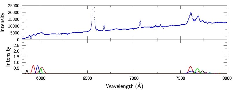
Figure 1: Optical spectrum of SS 433 on Julian day +260.5. The upper panel shows the spectrum after wavelength calibration and removal of the atmospheric telluric features and, in addition to the “moving” Balmer H$\alpha$ lines, shows the “stationary” H$\alpha$ line, as well as HeI and CII lines. The lower panel shows the gaussian fits to the moving H$\alpha$ lines after dividing through by a function fitted to the line-subtracted continuum background.

Stationary lines were removed from this analysis and moving lines identified as He or probable Paschen series hydrogen lines were also deleted from the present study. The remaining lines were taken as Balmer H$\alpha$ associated with the jet activity. These are shown day by day in Fig. 2, where each vertical mark has a height given by the logarithm of the product of peak height and standard deviation of the fitted gaussian. The multiple ejections most days are striking and we refer to each such ejection as a bolide. It is very clear that the scatter in measured wavelengths of bolides within a given day is substantially greater in the West jet than in the East for precessional phase near zero. It is also the case that the widths of the individual lines are similarly greater in the West than in the East, although that is not displayed here; see Fig. 9 in Section 5. The nodding motion is visible for the East jet, but because of the spread in the West jet the nodding is not as easy to see there, but is clearly seen in the plot of weighted means shown in Fig. 3.

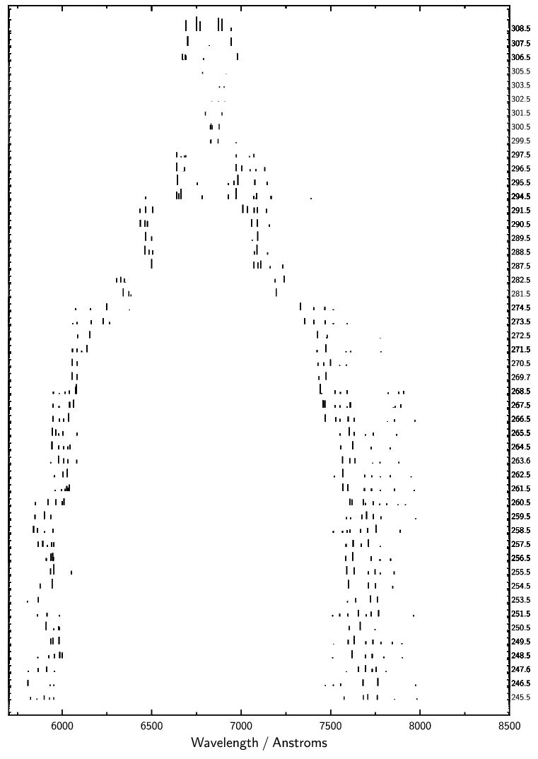
Figure 2: The central wavelengths of ejected bolides are displayed day by day. Each horizontal series is from a single spectrum; Julian Day increases vertically. The height of each bar is the area of the fitted gaussian, on a logarithmic scale. The scatter in central wavelengths is much greater in the right-hand (West) jet than the left-hand (East) jet and nodding is apparent, especially clearly in the left-hand (East) jet.

3 Properties revealed by averaging within a day

For each jet in each spectrum we calculated the mean wavelength of the bolide complex, that is, the mean of the wavelengths of the individual bolides weighted by their respective areas. Each spectrum was thus represented by a single pair of wavelengths as is the case for most archival data, some of which are of low spectral resolution. The redshift history of these means is shown in Fig. 3. The nodding is very clear in both jets and mirror symmetry is pronounced until after day 274. After day 285, both jets drift first in the direction of decreasing redshift and then increasing redshift, which could be (and probably is) due to decreasing and then increasing speed over durations of many days of the kind imaged by Blundell & Bowler (2004).

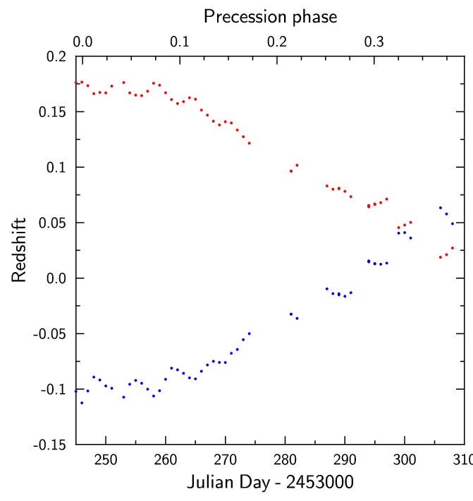
Figure 3: The daily weighted mean redshifts of the ejecta in each jet as a function of time. The nodding is very clear in both jets and after day 285 both drift first to the blue and then to the red.

Under the assumption that the variation in jet parameters is perfectly symmetric, the ejection speed can be extracted from the sum of the two redshifts (Blundell & Bowler, 2005) (see also Marshall et al 2002). These derived speeds are shown as a function of time in Fig. 4, where indeed the sustained higher speeds beyond day 294 are apparent. There is a trace of an approximately 13-day period in these speeds. To investigate how robust this is, we took the spectra up to and including day 274 (before the later long term drifts set in) and folded over 13.08 days, dividing the orbital phase into 5 bins. The data and fitted curve are shown in Fig. 5 (lower panel). The signal is significant and the parameters are:

• Mean speed $0.260\pm 0.002\,c$

• Amplitude of speed variation $0.006\pm 0.001\,c$

• Orbital phase of maximum speed $0.55\pm 0.03\times 2\pi$ (using the orbital phase convention of Goranskii et al. (1998)).

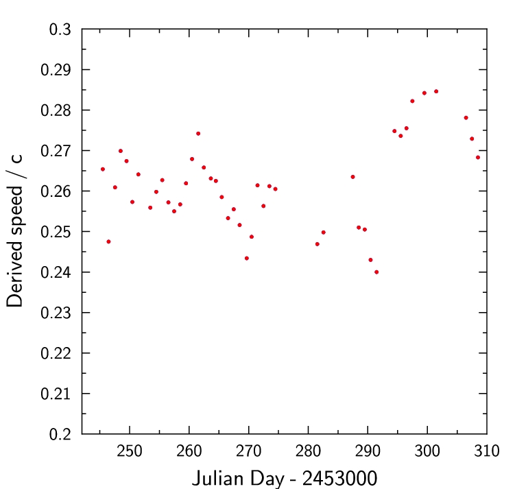
Figure 4: If the mean redshifts in each jet are produced by identical variations of speed and angle, the common speed can be calculated from the sum of the redshifts. This figure displays the speeds so calculated. Speeds are abnormally high after day 294 and a 13-day periodicity is readily discernable.

The mean speed and the amplitude of speed variation are in excellent agreement with those obtained from archival optical data (Blundell & Bowler, 2005). However, the phase is considerably different. The analysis of these new data thus drew our attention to the orbital phase of peak velocity, a parameter we had not previously investigated. We therefore refitted the archival data (Collins’ data set) and were careful to use the exact Goranskii ephemeris. The results (see Fig. 5, upper panel) were:

• Mean speed $0.2581\pm 0.0005\,c$

• Amplitude of speed variation $0.0063\pm 0.0010$ c

• Phase of maximum speed $0.230\pm 0.025\times 2\pi$

The Goranskii ephemeris is tied down by well-defined primary eclipses observed over the period 1978 – 1982 which dominates the archival data. The visible effects of the primary eclipses on the continuum background of our own data, presented in this paper, establish the validity of the Goranskii ephemeris to an accuracy of better than a day for our observations near the end of 2004. There is no doubt that the phase of the oscillation in jet speed has shifted over a quarter of a cycle between about 1980 and 2004.

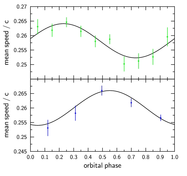
Figure 5: The figure shows the variation of jet speed, calculated from the sum of red shifts, folded over orbital phase bins, for (upper panel) the archival data and (lower panel) our 2004 data. Both sets show an orbital periodicity of the same amplitude, but the phases are different. The curves correspond to the fitted parameters listed in the text.

This 13-day periodicity occurs in the sum of $z_{+}$ and $z_{-}$, which is a maximum at orbital phase 0.23 in the archival data (dominated by 1978 – 1982) and 0.55 in the present data (observed 2004). If interpreted as a variation in ejection speed, the ejection speed had maxima at orbital phases 0.23 and 0.55 respectively. There are, however, alternative explanations for a periodicity in the sum of the redshifts. Perhaps the most obvious is simple Doppler shifting as a result of the orbital motion of the compact object. If this were the explanation the orbital speed would have to be in excess of 400 km s^-1 (Blundell & Bowler, 2005) but in fact this explanation is ruled out by the phases: at an orbital phase of 0.25, the compact object emerged from behind the companion star about a quarter of a revolution previously and so is approaching the observer; $z_{+}+z_{-}$ should be a minimum rather than the observed maximum. The phase of the peak speed would also be fixed with respect to the orbital phase.

A further possible explanation for a 13-day periodicity in the sum of $z_{+}$ and $z_{-}$ also has problems with the phase difference between the archival and our 2004 data. Suppose that rather than being ejected anti-parallel, the two jets are each deflected from the common jet axis of the kinematic model by about 1 degree, always in a direction towards the companion. That could do it for the data in this paper, where the sum has a maximum at orbital phase $\sim$0.5. However, the plane containing the two jets could not follow the companion perfectly because of the different phase observed 25 years ago. The data are not sufficient to reveal whether the phase advances steadily or can wander, but the existence of side bands having periods of 12.58 and 13.37 days in the archival data (Blundell & Bowler, 2005, fig. 3) suggests the latter.

Finally, there is the possibility that the ejection speed itself really does vary with a period of 13.08 days, perhaps as a result of Roche lobe overflow with a slightly eccentric orbit. If so, that orbit must have experienced a periastron advance of about 90 degrees in 25 years. Whatever the mechanism may be, the observation of a 13-day periodicity in the sum of $z_{+}$ and $z_{-}$ may be revealing an important property of the machinery whereby bulk plasma is accelerated to one quarter of the speed of light.

4 Fluctuations in redshift within a single jet

Variation of the wavelength of the emitted radiation due to thermal or bulk motion in a bolide rest frame can be handled as described by eqns.(2-11) in this section, but for the case of spherical symmetry in the bolide rest frame the observed line widths can also be attributed to a spread in proper wavelength. The observed line widths are too great for thermal broadening since they would imply temperatures greatly in excess of $10^{4}$ K.

Fluctuations in the wavelength emitted from a given jet might be due to variation of speed within that jet, of polar angle $\theta$ or of azimuthal angle $\phi$. (We discount the possibility of the angle of inclination of the precession axis, $i$ in equation 1, varying.) Differentiating equation 1 we have

$$\Delta z_{+} = F_{+}(\beta,\theta,\phi)\Delta\beta_{+}+G(\beta,\theta,\phi)\Delta\theta_{+}+H(\beta,\theta,\phi)\Delta\phi_{+}$$ (2)

$$\Delta z_{-} = F_{-}(\beta,\theta,\phi)\Delta\beta_{-}-G(\beta,\theta,\phi)\Delta\theta_{-}-H(\beta,\theta,\phi)\Delta\phi_{-}$$ (3)

where the same partial differentials $G$ and $H$ occur for both jets, but because of the transverse Doppler effect $F_{+}$ and $F_{-}$ are different. It is particularly important that when $\phi$ is approximately zero $F_{+}$ is much larger than $F_{-}$. The quantities $F{\pm}$, $G$ and $H$ are explicitly:

$$F{\pm} = \beta\gamma^{3}{\pm}\gamma^{3}f_{1}$$ (4)

$$G = \beta\gamma f_{2}$$ (5)

$$H = \beta\gamma f_{3}$$ (6)

where the angular functions are given by

$$f_{1} = \sin\theta\sin i\cos\phi+\cos\theta\cos i$$ (7)

$$f_{2} = \cos\theta\sin i\cos\phi-\sin\theta\cos i$$ (8)

$$f_{3} = -\sin\theta\sin i\sin\phi.$$ (9)

If equations 2 and 3 are each squared and we perform some appropriate average over the redshift excursions for given (small range of) $\phi$, the observed $\langle\Delta z_{+}^{2}\rangle$ are then parametrised in terms of 6 quantities $\langle\Delta\beta_{+}^{2}\rangle$, $\langle\Delta\theta_{+}^{2}\rangle$, $\langle\Delta\theta_{+}\Delta\beta_{+}\rangle$ and so on. Each of these six quantities is multiplied by a known function of the precessional phase angle $\phi$. The explicit dependences on $\phi$ are given in eqns 10 and 11 below and the dependence of terms multiplying $\langle\Delta\beta^{2}\rangle$ and $\langle\Delta\beta\Delta\theta\rangle$ is shown in Fig. 6. Fig. 6 (upper panel) is in fact a different representation of figure 1 in Katz & Piran (1982).

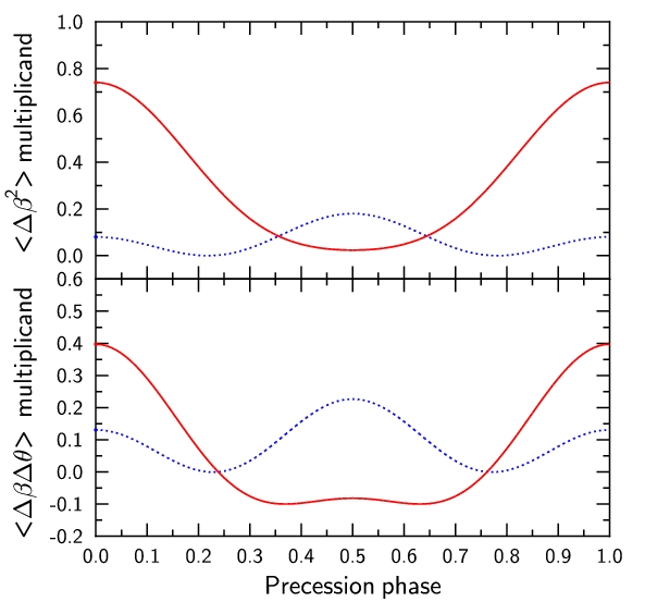
Figure 6: The dependences on precessional phase of the terms in eqns. 10 and 11 which are multiplied by $\langle\Delta\beta^{2}\rangle$ (upper panel) and $\langle\Delta\beta\Delta\theta\rangle$ (lower panel). The East jet ($-$) is indicated in (broken) blue and the West (+) in (solid) red.

Then $\langle\Delta z_{+}^{2}\rangle$ is parametrised by

$$\langle\Delta z_{+}^{2}\rangle = (\beta\gamma^{3}+\gamma^{3}f_{1})^{2}\langle\Delta\beta_{+}^{2}\rangle$$

$$+ (\beta\gamma f_{2})^{2}\langle\Delta\theta_{+}^{2}\rangle$$

$$+ (\beta\gamma f_{3})^{2}\langle\Delta\phi_{+}^{2}\rangle$$

$$+ 2(\beta\gamma^{3}+\gamma^{3}f_{1})(\beta\gamma f_{2})\langle\Delta\beta_{+}\Delta\theta_{+}\rangle$$

$$+ 2(\beta\gamma^{3}+\gamma^{3}f_{1})(\beta\gamma f_{3})\langle\Delta\beta_{+}\Delta\phi_{+}\rangle$$

$$+ 2(\beta\gamma f_{2})(\beta\gamma f_{3})\langle\Delta\theta_{+}\Delta\phi_{+}\rangle,$$

and $\langle\Delta z_{-}^{2}\rangle$ is parametrised by

$$\langle\Delta z_{-}^{2}\rangle = (\beta\gamma^{3}-\gamma^{3}f_{1})^{2}\langle\Delta\beta_{-}^{2}\rangle$$

$$+ (\beta\gamma f_{2})^{2}\langle\Delta\theta_{-}^{2}\rangle+(\beta\gamma f_{3})^{2}\langle\Delta\phi_{-}^{2}\rangle$$

$$- 2(\beta\gamma^{3}-\gamma^{3}f_{1})(\beta\gamma f_{2})\langle\Delta\beta_{-}\Delta\theta_{-}\rangle$$

$$- 2(\beta\gamma^{3}-\gamma^{3}f_{1})(\beta\gamma f_{3})\langle\Delta\beta_{-}\Delta\phi_{-}\rangle$$

$$+ 2(\beta\gamma f_{2})(\beta\gamma f_{3})\langle\Delta\theta_{-}\Delta\phi_{-}\rangle.$$

Thus given enough data of sufficient precision it would be possible to determine all 6 quantities $\langle\Delta\beta_{+}^{2}\rangle$ etc for the West jet and independently determine the analogous 6 quantities for the East jet. No assumption of symmetry would then be required and if the average $\langle\Delta\beta_{+}^{2}\rangle$ did actually differ from $\langle\Delta\beta_{-}^{2}\rangle$ that would be revealed by the data.

Unfortunately data sufficiently extensive and of such quality are not available. It is however possible to determine parameters such as $\langle\Delta\beta^{2}\rangle$ taken to be common to the two jets on average only, without the extreme assumption of symmetry in every ejection event (which we nonetheless believe to be a very good approximation). We first apply this treatment to the archival data and show that it leads to essentially identical results as the assumption of maximal symmetry (variations in the parameters common to both jets) employed in Blundell & Bowler (2005). In figure 6 of that paper it was shown that the description of fluctuations in the jets extracted assuming instantaneous symmetry also gave a very good description of the plot of observed $\Delta z_{-}$ versus $\Delta z_{+}$ i.e. numbers extracted from the data without any assumption of symmetry of any kind. An unexpected result of Blundell & Bowler (2005) was a strong anti-correlation between $\Delta\beta$ and $\Delta\theta$. It was pointed out (quite correctly) by H. Marshall (private communication to KMB) that if speed variations are asymmetric then an assumption of symmetry would introduce a specious anti-correlation. This of course does not mean that an anti-correlation is specious: if symmetry is true the anti-correlation is real.

In fact the $\phi$ dependence of $\Delta z_{+}^{2}$ and $\Delta z_{-}^{2}$ requires both fluctuations in speed and also separately an anti-correlation between $\Delta\beta$ and $\Delta\theta$, if it be admitted only that the parameters averaged over many years are the same for both jets (that is, $\langle\Delta\beta_{+}^{2}\rangle$ = $\langle\Delta\beta_{-}^{2}\rangle$ and so on for the other five pairs of parameters). Then subtracting equation 11 from equation 10, the difference of squared redshifts averaged over precessional phase is given by

$$\langle\Delta z_{+}^{2}\rangle-\langle\Delta z_{-}^{2}\rangle =$$ (12)

$$4\beta\gamma^{6}\cos\theta\cos i\langle\Delta\beta^{2}\rangle-4\beta^{2}\gamma^{4}\sin\theta\cos i\langle\Delta\beta\Delta\theta\rangle =$$

$$0.252\langle\Delta\beta^{2}\rangle-0.022\langle\Delta\beta\Delta\theta\rangle.$$

Under these assumptions the difference between $\Delta z_{+}^{2}$ and $\Delta z_{-}^{2}$ is given only by the terms in $\langle\Delta\beta^{2}\rangle$ and in $\langle\Delta\beta\Delta\theta\rangle$ and the latter term is very small. Fig. 7 shows the measured difference in $\Delta z_{+}^{2}$ and $\Delta z_{-}^{2}$ as a function of $\phi$ from Eikenberry’s archival data set; similar results are obtained with the data of Collins. The difference in $\Delta z_{+}^{2}$ and $\Delta z_{-}^{2}$ averaged over all $\phi$ is positive and has value $0.34\pm 0.08\times 10^{-4}$ (for red alone — i.e. $\Delta z_{+}^{2}$ — the value is $1.22\pm 0.09\times 10^{-4}$) and the difference between the red and blue jets is largest for precessional phase 0.5. Because the term in $\langle\Delta\beta\Delta\theta\rangle$ averaged over precessional phase is close to zero, the observed difference requires a root mean square speed fluctuation of about 0.01 $c$, regardless of the presence or otherwise of any correlation between $\Delta\beta$ and $\Delta\theta$.

Then comparison of Fig. 7 with Fig. 6 shows that to produce the largest difference at precessional phase 0.5 rather than zero absolutely requires an anti-correlation between $\Delta\beta$ and $\Delta\theta$ of about the size reported in Blundell & Bowler (2005). The curve superimposed on Fig. 7 is for $\langle\Delta\beta^{2}\rangle=1.67\times 10^{-4}$ and for $\langle\Delta\beta\Delta\theta\rangle=-3.8\times 10^{-4}$. It is also the case that $\langle\Delta z_{+}^{2}\rangle$ is larger near a phase of 0.5 than for phase close to zero, implying that a substantial anti-correlation is necessary in the red jet at least. The anti-correlation between $\Delta\theta$ and $\Delta\beta$ is thus shown to be no artifact of the assumption of instantaneous symmetry made in Blundell & Bowler (2005). However, an argument that the two jets are long term different cannot be refuted by the available Doppler data alone, but we repudiate it on the grounds of the recent radio image (Blundell & Bowler, 2004).

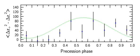
Figure 7: The difference between the mean square fluctuations in redshift for the West jet and the East jet, as a function of precessional phase, averaged over many cycles in the archival data. The vertical scale is in units of $10^{-6}$. Averaged over all phases the red (West, +) jet has larger fluctuations than the blue (East, $-$). If the two jets are on average symmetric, this requires fluctuations in speed. The difference is small near precession phase zero and largest near phase 0.5; comparison with Fig.6 shows that this requires a strong anti-correlation between speed and direction. The curve is the prediction of Blundell & Bowler (2005), rather than a fit.

Table 1: Comparison of short timescale fluctuations with long term deviations. Notes to Table. 1) The deviations in columns 2 and 3 were fitted to data internal to jets on a given day, measuring deviations from a local mean. The numbers in the last column represent deviations from the simple kinematic model and are from the fits of Blundell & Bowler (2005), assuming instantaneous symmetry. These numbers are also entirely consistent with analysis of those data assuming only that many year averages are equivalent for the two jets. 2) The last row gives the correlation coefficient between $\Delta\beta$ and $\Delta\theta$, defined as $\langle\Delta\beta\Delta\theta\rangle/\sqrt{\langle\Delta\beta^{2}\rangle\langle\Delta\theta^{2}\rangle}$.

fluctuating quantity	within bolides	among bolides	archival w.r.t kinematic model
$\langle\Delta\beta^{2}\rangle$	$(0.08\pm 0.01)\times 10^{-4}$	$(1.10\pm 0.20)\times 10^{-4}$	$(1.67\pm 0.18)\times 10^{-4}$
rms $\Delta\beta$	0.0028	0.01	0.013
$\langle\Delta\theta^{2}\rangle$	$0.8\pm 0.1\times 10^{-4}$	$(1.5\pm 0.4)\times 10^{-4}$	$(22.4\pm 3.5)\times 10^{-4}$
rms $\Delta\theta$	0.5 degrees	0.7 degrees	2.71 degrees
$\langle\Delta\theta\Delta\beta\rangle$	$(0\pm 0.02)\times 10^{-4}$	$(0\pm 0.25)\times 10^{-4}$	$(-3.81\pm 0.52)\times 10^{-4}$
correlation coefficient	$\sim 0$	$\sim 0$	$\sim-0.62$

5 Short timescale variations in the jets of SS 433

We have examined two measures of short timescale variations in the jets of SS 433, only possible because of the frequently-sampled high quality spectra at our disposal. Both of these measures reveal patterns which have simple and natural explanations if the average properties of the two jets are the same. Fig. 2 shows the pattern of multiple resolved lines on any given night and one measure of short timescale variation is the scatter of these lines in each jet in each spectrum.

For the bolides observed in each jet on each night we calculated the area-weighted mean square deviation in redshift of the individual lines from the weighted average of all observed that night. This quantity, the variance, is plotted in Fig. 8 as a function of the precessional phase. The units are (dimensionless) redshift with a factor of $10^{-6}$ extracted. There is a good deal of scatter from day to day, but several features are clear. First, near precession phase zero the West (red) has a much greater scatter in redshift than the East (blue), by a factor of 4 or so. Second, the red and blue fluctuations converge as the precession phase advances towards $0.4\times 2\pi$. Finally, both the red and the blue means decrease from phase zero toward phase 0.3. Comparison of Fig. 8 with Fig. 6 (upper panel) shows that these features are all characteristic of about equal rms fluctuations in each jet, dominated by variation of the ejection speed.

The second measure is, for each jet on each day, the area-weighted mean of the squares of the standard deviations of the gaussians (in units of redshift with $10^{-6}$ extracted) fitted to the individual bolides. This quantity, $\sigma^{2}$, is plotted in Fig. 9 as a function of precession phase. Here again the mean square excursions are larger in the West (red) jet than in the East (blue) near phase of zero and the two converge as the phase advances. In this instance the mean blue is rising as the mean red falls. Again the role of speed fluctuations must be important but their magnitude is much smaller than for Fig. 8; pointing jitter dominates in the East jet. In fact, this pattern is close to — and could be — that from spherically symmetric expansion in the rest frames of the individual bolides, on average the same in the two jets.

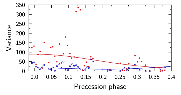
Figure 8: The scatter of bolide redshifts, measured by the weighted variance discussed in the text, as a function of precession phase. The vertical scale is in units of $10^{-6}$. The West jet is indicated by red, solid symbols; the East jet by blue, open symbols. The curves are constructed from eqns. 10 and 11, with the parameters listed in Table 1. The red and blue patterns in conjunction bear the signature of dominant fluctuations in speed; see Fig. 6.

These data shown in Figs 8 and 9 are scattered in variance and $\sigma^{2}$ respectively, but do not extend beyond precessional phase of $0.4\times 2\pi$; in order to quantify the contents of Figs. 8 and 9 we made the following assumptions. First, we assumed that the quantities $\langle\Delta\beta^{2}\rangle$, $\langle\Delta\beta\Delta\theta\rangle$ and so on, the averages being taken over a few days (rather than over many years as for the archival data) are common to both jets, as suggested by the distinctive patterns in those figures. Second, we assumed that the rms value of $\Delta\phi$ is given by the rms value of $\Delta\theta$, divided by $\sin\theta$. This is the condition for “pointing jitter” (Katz & Piran, 1982) and was satisfied in analysis of the archival data in Blundell & Bowler (2005) whether or not the jets were required to be anti-parallel. We also assumed that the averages $\langle\Delta\beta\Delta\phi\rangle$ and $\langle\Delta\theta\Delta\phi\rangle$ could be neglected. The data in both jets were thus represented in terms of three parameters $\langle\Delta\beta^{2}\rangle$, $\langle\Delta\theta^{2}\rangle$ and the correlation parameter $\langle\Delta\beta\Delta\theta\rangle$. The raw data-points shown in Figs. 8 and 9 were averaged within 10 bins of precessional phase, the errors on the means taken from the variance of the entries within a bin (but set very large in the rare cases where a bin contained only two entries or less) and the $\chi^{2}$ minimised in terms of those three fluctuation parameters. The resulting smooth curves are shown in Figs. 8 and 9 and the extracted parameters summarised in Table 1 and compared with the parameters from the archival data. The simple model assuming average symmetry of the two jets provides as good a description of these data as anyone could desire.

It is however the case that the features of Fig. 8 could be explained by fluctuations dominated by $\Delta\theta$ provided that such fluctuations are systematically greater (by more than a factor of two) in the West jet than in the East. Similarly, the features of Fig. 9 could be explained by systematically different variations of $\Delta\theta$ and $\Delta\phi$ in the two jets. However, such explanations are contrived and unnatural.

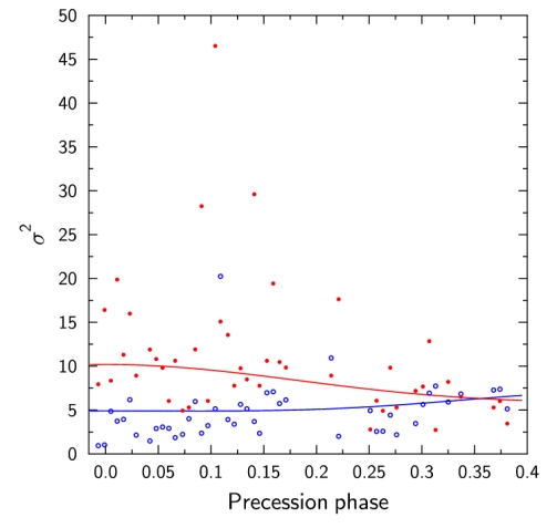
Figure 9: The spread of the widths in redshift of the lines observed from individual bolides, as measured by the square of the standard deviation of the fitted gaussians, displayed as a function of precessional phase. The East jet is indicated by blue, open symbols and the West by red, solid symbols. The curves are constructed from the parameters listed in Table 1. The blue distribution is rising to meet the red; this corresponds to relatively small fluctuations in speed. If the two jets each contain bolides expanding spherically in the bolide rest frame, much the same pattern would be generated, in which case the magnitude of the red curve would be reduced by about a factor of 0.8. The vertical scale is in units of $10^{-6}$.

6 Bulk motion and expansion of the plasma

Material within an individual ejection (a single bolide or gaussian fit from our 2004 Chile data) on average has has an rms angular spread of about half a degree. There is a significant spread in speed but much smaller than the difference in speeds of separate bolides emitted within a day or so. This is hardly surprising since it is required that bolides be resolved. Over a day or so the ejection speeds of successive individual bolides vary by more than 0.01 $c$ and this variation is close to the rms deviation from the kinematic model in the archival data. However, the observed spread of angular deviations within a day is a factor of 4 smaller. It would seem that it is much easier to eject different speeds within a day than to twist the nozzles on the same timescale, perhaps not surprising if the nozzles are embedded in a disc with enormous moment of inertia. There is no significant anti-correlation between $\Delta\beta$ and $\Delta\theta$ within a single bolide; nor between bolides within a single day. In contrast, there is substantial (anti-) correlation in deviations from the kinematic model, sensitive to much longer timescale effects.

The data on the spread within individual bolides are consistent with a rather simple picture. The curves shown in Fig. 9 are for a combination of speed fluctuations and pointing jitter within individual bolides. The corresponding numbers listed in Table 1 show longitudinal speed variations of rms value 0.0028 $c$ and rms transverse speed variations of 0.0023 $c$. This transverse speed is $\beta$ (0.26 $c$) multiplied by the rms angular spread (the square root of $\langle\Delta\theta^{2}\rangle$) extracted from Fig. 9. The curves for the two jets also converge in just the same way that the redshifts themselves converge. Thus these data suggest that the “within bolide” characteristics are those of optically thin fireballs expanding with spherical symmetry within their own rest frames. If this model is imposed on these data the rms speed of expansion is 0.0024$\,c$, greatly in excess of any plausible thermal speeds.

It is a pity that SS 433 became a day-time object before a precessional phase of even 0.4 was reached; completing half a precessional rotation should have been much more informative because according to the model fit the East (or left or blue) jet would have exhibited inter-bolide variations exceeding those in the West (or right or red) jet in the vicinity of precession phase 0.5. The consistency of the simple model (in which the two jets are equivalent at least on average and speed fluctuations are present) with these new data is nonetheless compelling.

7 Conclusions

The jets of SS 433 exhibit fluctuations in direction and in speed on all time scales measured thus far. The new data reported here reveal, for material within individual bolides, an rms angular spread of about 0.5 degrees, with rms (longitudinal) speed fluctuations of 0.0028 $c$, rather like spherical expansion of optically thin bolides in their own rest frames. Where resolved bolides are produced within the same 24-hour period, the rms pointing jitter of those bolides is only a little larger, 0.7 degrees, but the spread of speeds is about 0.01 $c$. There is no evidence that material within single bolides shows an anti-correlation between $\Delta\beta$ and $\Delta\theta$, nor between bolides on short timescales of order one day collectively exhibit such anti-correlation.

These results depend on assuming that the East and West jets are equivalent averaged over periods of a few days or less, but do not require instantaneous symmetry. The analysis of archival data in Blundell & Bowler (2005) assumed instantaneous symmetry and that analysis described well the archival data with rms angular deviations from the kinematic model of 2.7 degrees and rms speed fluctuations of 0.013 $c$, with a correlation coefficient of $-0.62$. In this paper we have shown that these results are also obtained assuming only that the two jets are equivalent when averaging over the many year timescale of the archival data. There can now be little doubt that the two jets are highly symmetric on timescales longer than a day or two; the extent to which the jets are symmetric on timescales of a day or less cannot be answered without high precision sampling of the optical spectrum as frequently as every few hours.

It is extremely interesting that the speed variations exhibited by multiple bolides within a day (rms 0.01 $c$) are pretty much identical to the speed variations on much longer timescales (Blundell & Bowler, 2004, 2005) yet the associated angular fluctuations are much smaller on timescales of order one day. It is also interesting that any correlations between angular and speed fluctuations are of much smaller magnitude on the shorter time scales. These observations alone make it unlikely that angular tilts, in for example the disc, control the perceived ejection speed (Begelman et al., 2006) but it might be that sustained higher speed ejection is capable of reaming out the nozzle in the disc and so decreasing the polar angle.

It should be emphasised that the physical origin of the anti-correlation between $\Delta\beta$ and $\Delta\theta$ in the long term data (correlation coefficient = $-0.62$) is quite unknown – but we have now demonstrated clearly that this result of Blundell & Bowler (2005) is not an artifact of the assumption of instantaneously symmetric ejection speeds as there employed.

In a recent paper, Begelman et al. (2006) suggested that this anti-correlation might be produced by the jets impacting on the walls of the core of the disc and if they retained only that component of speed parallel to the walls. However, this is inconsistent with the archival data and the 2004 data presented here, because the angular fluctuations are not big enough to produce the associated speed fluctuations. In the model of Begelman et al. (2006) the emergent jet velocity is given by

$$\beta=\beta_{0}\cos\theta$$ (13)

where $\beta_{0}$ is a constant speed before impact on the walls and hence

$$\Delta\beta=-\beta_{0}\sin\theta\Delta\theta$$ (14)

Then $\langle\Delta\beta^{2}\rangle$ would be approximately equal to 0.01 $\langle\Delta\theta^{2}\rangle$ and this relationship is completely inconsistent with Table 1. In addition, if some trace of this mechanism were in operation the nodding frequency would appear in the sum of $z_{+}$ and $z_{-}$ but it does not (Blundell & Bowler, 2005). The new observation of negligible correlation on short time scales further rules out the explanation suggested by Begelman et al. (2006).

The multiple ejections within a single day and their properties are themselves of great interest, and we have shown that for the purposes of pairing ejecta even the area-weighted mean redshifts contain a great deal of information; they exhibit beautifully symmetric nodding and also systematic drifts associated with longer-term speed changes. We found that the interval from day 245 to 274 showed a clear periodicity of 13 days in the sum of $z_{+}$ and $z_{-}$, with maximum excursion in the 2004 data when the compact object and the companion both lie along the line of sight. In the archival data (Blundell & Bowler, 2005) the maximum excursion is a quarter of a cycle earlier (dominated by observations of 25 years ago) but in both cases the maximum excursion is in quite the wrong place for this periodicity to be a Doppler effect due to the orbital speed of the compact object. To obtain greater insight, it is necessary to mount a campaign of at least daily observations sustained over some years.