Quantum and classical criticalities in the frustrated two-leg Heisenberg ladder

Abstract

This talk was about the frustration-induced criticality in the antiferromagnetic Heisenberg model on the two-leg ladder with exchange interactions along the chains, rungs, and diagonals, and also about the effect of thermal fluctuations on this criticlity. The method used is the bond mean-field theory, which is based on the Jordan-Wigner transformation in dimensions higher than one. In this paper, we will summarize the main results presented in this talk, and report on new results about the couplings and temperature dependences of the spin susceptibility.

I Introduction

We use the bond-mean-field theory (BMFT), which is based on the Jordan-Wigner (JW) transformation, to study the quantum criticality phenomenon in the frustrated antiferromagnetic (AF) two-leg Heisenberg ladder, and the effect of temperature on this criticality Azz1 ; Azz2 ; Azz3 ; Azz5 ; ramakko2007 . This method has been applied to the Heisenberg single chain, two-leg ladder, and three-leg ladder without frustration with excellent results azzouz2005 . When the diagonal interaction is varied the two-leg ladder system can undergo a quantum phase transition between two of three distinct non-magnetic quantum spin liquid states; the Néel-type (N-type) state, ferromagnetic-type rung (R-type) state, and ferromagnetic-type chain (F-type) state. These states are characterized by ferromagnetic spin arrangements along the diagonals, rungs, or chains respectively. The BMFT is a mean-field theory that is based on the spin bond parameters. The latter are related to the spin-spin correlation function $\langle S_{i}^{-}S_{j}^{+}\rangle$, with $i$ and $j$ labeling two adjacent sites in the direction where this correlation function is calculated. All quantities $\langle S_{i}^{\alpha}\rangle$, with $\alpha=x,\ y,\ z$, are zero in BMFT, implying the absence of any sort of long-range magnetic order.

The Hamiltonian for the spin-$\frac{1}{2}$ two-leg ladder with diagonal interactions is written as

$$H=J\sum_{i}^{N}\sum_{j=1}^{2}\textbf{S}_{i,j}\cdot\textbf{S}_{i+1,j}+J_{\perp}\sum_{i}^{N}\textbf{S}_{i,1}\cdot\textbf{S}_{i,2}+J_{\times}\sum_{i}^{N}(\textbf{S}_{i,1}\cdot\textbf{S}_{i+1,2}+\textbf{S}_{i+1,1}\cdot\textbf{S}_{i,2}),$$ (1)

where $J$ is the coupling along the chains, $J_{\perp}$ the coupling along the rungs, and $J_{\times}$ the coupling along the diagonals as seen in Fig. 1. The index $i$ labels the position of the spins along the two chains, each of which has $N$ sites, and $j$ labels the chains. As usual, $\textbf{S}_{i,j}$ is the spin operator.

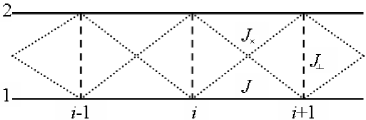
Figure 1: The two-leg ladder showing the couplings along the chains, rungs, and diagonals is displayed.

The frustrated two-leg ladder has been studied numerically using the Ising and dimer expansions Jd6 , the Lanczos diagonalization technique Jd6 ; Jd11 ; Jd4 ; Jd8 , and the density-matrix renormalization group (DMRG) Jd8 ; white1996 ; Jd5 ; Jd10 ; Jd3 . It has also been studied analytically using the bosonization Jd6 ; Jd13 , the valence-bond spin wave theory Jd7 , a non-perturbative effective-field theory Jd9 , the non-linear sigma model Jd12 , the reformulated weak-coupling field theory starykh2004 , and the Lieb-Mattis theorem hakobyan2007 . None of these analytical works addressed the issue of the phase diagram in all regimes including the weak, intermediate, and strong coupling limits. Within the BMFT, the phase diagram and its temperature dependence can be easily examined in all these regimes.

This paper is organized as follows. In Sec. II, we explain how the BMFT, which is based on the JW transformation in dimensions higher than one, is applied to our Hamiltonian. The Quantum and classical critical behaviours, and the spin susceptibility are discussed in Sec. III. In Sec. IV, conclusions are reported.

II Method

The JW transformation for the two-leg Heisenberg ladder is defined as Azz3

$$S_{i,j}^{-} = c_{i,j}e^{i\phi_{i,j}},\ \ \ S_{i,j}^{z}=n_{i,j}-1/2,\ \ \ \ n_{i,j}=c_{i,j}^{{\dagger}}c_{i,j},$$

$$\phi_{i,1} = \pi[\sum_{d=0}^{i-1}\sum_{f=1}^{2}n_{d,f}]\ \ {\rm\ for\ chain\ 1,}$$

$$\phi_{i,2} = \pi[\sum_{d=0}^{i-1}\sum_{f=1}^{2}n_{d,f}+n_{i,1}]\ \ {\rm\ for\ chain\ 2}.$$ (2)

The $c_{i,j}^{{\dagger}}$ operator creates a spinless fermion at site $(i,j)$, while $c_{i,j}$ annihilates one, and $n_{i,j}$ is the occupation number operator at that site. The phases $\phi_{i,j}$ are chosen so that at the the spin operators commutation relations are preserved.

After applying the JW transformation (II) to the Hamiltonian (1) we get

$$H =\frac{J}{2}\sum_{i}^{N}(c_{i,1}^{{\dagger}}e^{i\pi n_{i,2}}c_{i+1,1}+c_{i,2}^{{\dagger}}e^{i\pi n_{i+1,1}}c_{i+1,2}+\textrm{H.c.})+\frac{J_{\perp}}{2}\sum_{i}^{N}(c_{i,1}^{{\dagger}}c_{i,2}+\textrm{H.c.})$$ (3)

$$+\frac{J_{\times}}{2}\sum_{i}^{N}(c_{i,1}^{{\dagger}}e^{i\pi(n_{i,2}+n_{i+1,1})}c_{i+1,2}+c_{i+1,1}^{{\dagger}}c_{i,2}+\textrm{H.c.})+J\sum_{i}^{N}\sum_{j=1}^{2}(n_{i,j}-\frac{1}{2})(n_{i+1,j}-\frac{1}{2})$$

$$+J_{\perp}\sum_{i}^{N}(n_{i,1}-\frac{1}{2})(n_{i,2}-\frac{1}{2})+J_{\times}\sum_{i}^{N}[(n_{i,1}-\frac{1}{2})(n_{i+1,2}-\frac{1}{2})$$

$$+(n_{i+1,1}-\frac{1}{2})(n_{i,2}-\frac{1}{2})].$$

In BMFT, the interacting terms of the JW fermions are decoupled using the spin bond parameters. This approximation neglects fluctuations around the mean field points; $(O-\langle O\rangle)(O^{\prime}-\langle O^{\prime}\rangle)\approx 0$, where $O$ and $O^{\prime}$ are any operators which are quadratic in $c^{\dagger}$ and $c$ Azz2 . This yields

$$OO^{\prime}\approx\langle O\rangle O^{\prime}+O\langle O^{\prime}\rangle-\langle O\rangle\langle O^{\prime}\rangle.$$ (4)

To apply BMFT we introduce three mean-field bond parameters; $Q$ in the longitudinal direction, $P$ in the transverse direction, and $P^{\prime}$ along the diagonal. These can be interpreted as effective hopping energies for the JW fermions Azz1 in the longitudinal, transverse and diagonal directions, respectively:

$$Q=\langle c_{i,j}c_{i+1,j}^{{\dagger}}\rangle,\qquad P=\langle c_{i,j}c_{i,j+1}^{{\dagger}}\rangle,\qquad P^{\prime}=\langle c_{i+1,j}c_{i,j+1}^{{\dagger}}\rangle.$$ (5)

Keeping in mind that there is no long-range order Mermin so that $\langle S_{i,j}^{z}\rangle=\langle c_{i,1}^{{\dagger}}c_{i,1}\rangle-1/2=0$, the Ising quartic terms in equation (3) can be decoupled using the Hartree-Fock approximation (4), and the bond parameters (5) as follows:

$$\left(c_{i,1}^{{\dagger}}c_{i,1}\!-\!\frac{1}{2}\right)\left(c_{i+1,1}^{{\dagger}}c_{i+1,1}\!-\!\frac{1}{2}\right) \approx Qc_{i,1}^{{\dagger}}c_{i+1,1}+Q^{*}c_{i+1,1}^{{\dagger}}c_{i,1}+|Q|^{2},$$ (6)

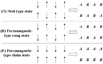
Figure 2: In the left panel, the three possible ground states of the system in the Ising limit, namely the Néel state, the ferromagnetic chain state, and the ferromagnetic rung state are drawn. In the right panel, the labeling of sublattices corresponding to the short-range spin orders that replace the long-range ones are shown for the Heisenberg limit.

for the Ising interaction along the chain 1. Similar equations can be obtained for the interactions along the other directions. Next, we write the Hamiltonian (3) using the three different spin configurations in the right panel of Fig. 2. These configurations are instantaneous (not static) configurations in which adjacent spins in any direction keep on average the same relative orientations with respect to each other, but fluctuate globally on a time scale determined by the strongest coupling constant so that any kind of long-range magnetic order is absent. These fluctuations are a consequence of the spin quantum fluctuations. The three competing configurations of Fig. 2 lead to three different quantum gapped spin liquid states, each characterized by its own short-range spin correlations and symmetry. We also choose to place an alternating phase of $\pi$ along the chains so that the phase per plaquette is $\pi$ Affleck . This phase configuration is used to get rid of the phase terms in the Hamiltonian. We also set $Q_{i,j}=Qe^{i\Phi_{i,j}}$ where $Q$ is site independent Azz5 . Here $\Phi_{i,j}$ is the phase of the bond along the chain; i.e., if $\phi_{i,j}=0$ on a given bond, then it is equal to $\pi$ on the adjacent ones. This is necessary in order to recover the proper result in the limit $J_{\times}$ and $J_{\perp}$ becoming zero, in which we get an energy spectrum comparable to that of des Cloiseaux and Pearson Cloiseaux for the spin excitation in a single Heisenberg chain, $E(k)=\frac{\pi}{2}J\left|\sin k\right|.$

For each state the Hamiltonian is written in the Nambu formalism and the matrix is diagonalized to obtain four eigenenergies (for each of the states). The details can be found in Ref. ramakko2007 . The eigenenergies for the N, F, and R-type states are given respectively by

$$E_{N}(k)\! \!=\! \!\pm\!J_{\times 1}\cos k\pm\sqrt{J_{1}^{2}\sin^{2}k+\frac{J_{\perp 1}^{2}}{4}},$$

$$E_{F}(k)\! \!=\! \!\pm J_{1}\cos k\pm\sqrt{J_{\times 1}^{2}\sin^{2}k+\frac{J_{\perp 1}^{2}}{4}},$$

$$E_{R}(k)\! \!=\! \!\pm\frac{J_{\perp 1}}{2}\pm\sqrt{J_{1}^{2}\sin^{2}k+J_{\times 1}^{2}\cos^{2}k},$$ (7)

where $J_{1}=J(1+2Q)$, $J_{\perp 1}=J_{\perp}(1+2P)$, and $J_{\times 1}=J_{\times}(1+2P^{\prime})$. The free energy per site is

$$F=JQ^{2}+\frac{J_{\perp}P^{2}}{2}+J_{\times}P^{\prime 2}-\frac{k_{B}T}{4N}\sum_{k}\sum_{p=1}^{4}\ln[1+e^{-\beta E_{p}(k)}],$$ (8)

where $E_{p}(k)$ is one of the four eigenenergies in any state. The minimization of the free energy with respect to the bond parameters leads to the following set of self-consistent equations:

$$Q = -\frac{1}{8NJ}\sum_{k}\sum_{p=1}^{4}\frac{\partial E_{p}(k)}{\partial Q}n_{F}[E_{p}(k)],$$

$$P = -\frac{1}{4NJ_{\perp}}\sum_{k}\sum_{p=1}^{4}\frac{\partial E_{p}(k)}{\partial P}n_{F}[E_{p}(k)],$$

$$P^{\prime} = -\frac{1}{8NJ_{\times}}\sum_{k}\sum_{p=1}^{4}\frac{\partial E_{p}(k)}{\partial P^{\prime}}n_{F}[E_{p}(k)],$$ (9)

which are solved numerically, except in the high-temperature regime, where analytical results are obtained.

III Results

The free (ground-state) energies of all three states are calculated as functions of the coupling constants and compared. From thermodynamic considerations the state with the lowest free energy is the stable one, and whenever free energies cross a phase transition takes place. Since only the ratios of the couplings are important we define $\alpha_{1}=J_{\perp}/J$ and $\alpha_{2}=J_{\times}/J$. In this way we have obtained the zero and finite temperature phase diagrams which can be seen in Fig. 3. The agreement between the Lanczos method data and our results is very good, a fact that indicates that the present mean-field treatment is acceptable. The line at $\alpha_{2}=1$ is exact and its placement is a consequence of the Hamiltonian symmetry with respect to exchanging $J$ and $J_{\times}$. The quantum phase transitions (zero temperature) found here using BMFT are first-order ones for all values of $\alpha_{2}$. As temperature increases the R-type state decreases in size. The sizes of the N-type and F-type phases increase with temperature. For any set of coupling values in the shaded region of Fig. 3b a classical (thermally induced) first order transition from the R-type state to one of the other states occurs ramakko2007 .

(a) (b)

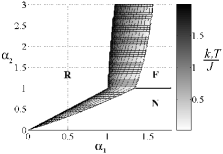
Figure 3: The zero-$T$ (a) and finite-$T$ (b) $(\alpha_{1},\alpha_{2})$-phase diagrams are shown. The zero-$T$ one is compared with the Lanczos-method Jd6 and the Ising limit. The boundaries are between the N-type state (N), R-type state (R), and the F-type state (F).

The uniform magnetic susceptibility $\chi(T)$ is calculated following the same method as Ref. Azz5 . It is plotted as a function of temperature in Fig. 4 . The Heisenberg model on a chain ($\alpha_{1}=0,\alpha_{2}=0$) is gapless whereas when $\alpha_{1}\neq 0$ and/or $\alpha_{2}\neq 0$ an energy gap opens up in the low-energy excitation. This is why at zero temperature $\chi\neq 0$ only for the chain, and an exponentially decreasing susceptibility is obtained for nonzero $\alpha_{1}$ or $\alpha_{2}$. For $\alpha_{1}=0.6$ and $\alpha_{2}=0.5$ there is a sudden transition from the R-type state to the N-type state at $k_{B}T/J=0.39$. For example, for $\alpha_{1}=1.25$ and $\alpha_{2}=2$ there is a sudden transition from the R-type state to the N-type state at $k_{B}T/J=0.64$. This sudden transition results in a discontinuity in $\chi$. These findings remain to be confirmed by others means.

(a) (b)

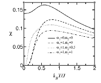
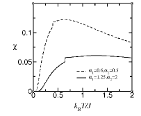
Figure 4: The uniform spin susceptibility $\chi(T)$ is plotted as a function of temperature for $h=0$ for several coupling constants.

IV Conclusion

In this talk, quantum and classical critical behaviours in the frustrated antiferromagnetic two-leg ladder were presented. The method of calculation, which is based on the Jordan-Wigner transformation and the bond-mean-field theory was explained. The zero-temperature phase diagram of this system was explained. It exhibits three quantum phases, characterized all by an energy gap and absence of magnetic order. These states are labeled Néel-type, Rung-type and Ferromagnetic-type chain states. Our zero-$T$ results agree well with existing numerical data. When temperature increases for some sets of coupling values, the system undergoes a phase transition from the R-type state to the N or F-type state at a finite temperature. The finite temperature phase diagram was explained as well. In it, the size of the R-type state becomes smaller while the F-type state and the N-type state increase in size with increasing temperature. Our theory predicts a discontinuity in the spin susceptibility at a finite temperature for the sets of couplings where the finite-$T$ transition occurs.

References

- (1) M. Azzouz, Phys. Rev. B 48, 6136 (1993).
- (2) B. Bock and M. Azzouz, Phys. Rev. B 64, 054410 (2001).
- (3) M. Azzouz, L. Chen, and S. Moukouri, Phys. Rev. B 50, 6233 (1994).
- (4) M. Azzouz, Phys. Rev. B 74, 174422 (2006).
- (5) B.W. Ramakko and M. Azzouz,Phys. Rev. B 76, 064419 (2007).
- (6) M. Azzouz and K.A. Asante, Phys. Rev. B 72, 094433 (2005).
- (7) Z. Weihong, V. Kotov, and J. Oitmaa, Phys. Rev. B 57, 11439 (1998).
- (8) M. Matsuda, K. Katsumata, R.S. Eccleston, S. Brehmer, and H.-J. Mikeska, J. Applied Phys. 87, 6271 (2000).
- (9) T. Sakai and N. Okazaki, Journal of Applied Physics 87, 5893 (2000).
- (10) H.-H. Hung, C.-D. Gong, Y.-C. Chen, and M.-F. Yang, cond-mat/0605719, (2006).
- (11) S.R. White, Phys. Rev. B 53, 52 (1996).
- (12) N. Zhu, X. Wang, and C. Chen, Phys. Rev. B 63, 012401 (2000).
- (13) T. Hakobyan, J.H. Hetherington, and M. Roger, Phys. Rev. B 63, 144433 (2001).
- (14) X.Q. Wang Mod. Phys. Lett. B 14, 327 (2000).
- (15) D. Allen, F.H.L. Essler, and A.A. Nersesyan, Phys. Rev. B 61, 8871 (2000).
- (16) Y. Xian, Phys. Rev. B 52, 12485 (1995).
- (17) D.C. Cabra, A. Dobry, and G.L. Rossini, Phys. Rev. B 63, 144408 (2001).
- (18) C-M Nedelcu, A. K. Kolezhuk, and H-J Mikeska, J. Phys.:Condens. Matter 12, 959 (2000).
- (19) O.A. Starykh and L. Balents, Phys. Rev. Lett. 93, 127202 (2004).
- (20) T. Hakobyan, cond-mat/0702148 (2007).
- (21) N.D. Mermin and H. Wagner, Phys. Rev. Lett. 17, 1133 (1966).
- (22) I. Affleck and J.B. Marston, Phys. Rev. B 37, 3774 (1988).
- (23) J. des Cloiseaux and J.J. Pearson, Phys. Rev. 128, 2131 (1962).