Single polaron properties of the breathing-mode Hamiltonian

Abstract

We investigate numerically various properties of the one-dimensional (1D) breathing-mode polaron. We use an extension of a variational scheme to compute the energies and wave-functions of the two lowest-energy eigenstates for any momentum, as well as a scheme to compute directly the polaron’s Green’s function. We contrast these results with results for the 1D Holstein polaron. In particular, we find that the crossover from a large to a small polaron is significantly sharper. Unlike for the Holstein model, at moderate and large couplings the breathing-mode polaron dispersion has non-monotonic dependence on the polaron momentum $k$. Neither of these aspects is revealed by a previous study based on the self-consistent Born approximation.

I Introduction

In a solid-state system, the interaction between a charge carrier and phonons (quantized lattice vibrations) leads to the formation of polarons. This mechanism is a key ingredient in the physics of the manganitesmanganite and, possibly, of the cuprates.cuprate ^,TomD There are various model Hamiltonians describing the coupling of the particle and bosonic degrees of freedom. The asymptotic limits of weak or strong coupling can be investigated analytically using perturbation theory, however the intermediate-coupling regime generally requires numerical simulations. Recently, investigations of basic model Hamiltonians have progressed rapidly thanks to the development of efficient analytical and computational tools, and we are now able to begin to study more and more realistic models.

The simplest electron-phonon coupling is described by the Holstein Hamiltonian.Holstein It is essentially the tight-binding model with an on-site energy proportional to the lattice displacement $X_{i}=\frac{1}{\sqrt{2M\Omega}}(b_{i}^{{\dagger}}+b_{i})$:

$$H_{H}=-t\sum_{<ij>}\left(c_{i}^{{\dagger}}c_{j}+c_{j}^{{\dagger}}c_{i}\right)+\Omega\sum_{i}b_{i}^{{\dagger}}b_{i}+g\sum_{i}n_{i}X_{i}$$ (1)

Here $c_{i}$ is the annihilation operator for an electron at site $i$ (since we only consider the single electron case, the spin is irrelevant and we drop its index in the following. We also set $\hbar=1$). $t$ is the hopping matrix, $n_{i}=c_{i}^{\dagger}c_{i}$. For the Einstein phonons, $b_{i}$ is the annihilation operator at site $i$, $\Omega$ is the frequency, $M$ is the atomic mass, and $g$ is the electron-phonon coupling strength. The model has been widely studied numerically by Monte-Carlo calculations,mc1 ^-mc12 variational methods,bonca ^-v18 and exact diagonalization.md1 ^-marsiglio Analytic approximations have also progressed over the years.a1 ; MA ; a2 ; a3

For some materials, a more appropriate model is provided by the breathing-mode Hamiltonian. For example, consider a half-filled 2D copper-oxygen plane of a parent cuprate compound. Injection of an additional hole should fill an oxygen $2p$ orbital. Due to hybridization between oxygen $2p$ and copper $3d_{x^{2}-y^{2}}$ orbitals, the hole resides in fact in a so-called Zhang-Rice singlet (ZRS) with a binding energy proportional to $-8t^{2}_{dp}$, where $t_{dp}$ is the hopping between neighboring O and Cu orbitals. The dynamics of the ZRS can be described by an effective one-band model with orbitals centered on the copper sub-lattice.ZR If lattice vibrations are considered, the motion of the lighter oxygen ions, which live on the bonds connecting Cu sites, are the most relevant. The hopping integral $t_{dp}$ and charge-transfer gap between Cu and O orbitals are now modulated as the oxygen moves closer or further from its neighboring Cu atom. Both the on-site energy and hopping integral are modulated in the effective one-band model, but the former has been shown to be dominantbr1 ^,br2 . The breathing-mode Hamiltonian describes the physics of the linear modulation of on-site energy.

While this breathing-mode model is motivated as a 2D model, in this work we investigate numerically only its 1D version, relevant, e.g. for CuO chains. In 1D we can investigate accurately and efficiently not only ground-state (GS) properties, but also some excited state properties. For the Holstein model, it was found that polaron properties are qualitatively similar in different dimensions,v6 ; a2 but with a sharper large-to-small polaron crossover in higher dimensions. We will show that a sharp crossover is already present in the 1D model, and we expect less dimensionality effects in the breathing-mode Hamiltonian.

The 1D breathing-mode Hamiltonian that we investigate here is described by:

$$H_{B}=-t\sum_{i}\left(c_{i}^{{\dagger}}c_{i+1}+c_{i+1}^{{\dagger}}c_{i}\right)+\Omega\sum_{i}b_{i+{1\over 2}}^{{\dagger}}b_{i+{1\over 2}}$$

$$+\frac{g}{\sqrt{2M\Omega}}\sum_{i}n_{i}\left(b_{i+{1\over 2}}^{{\dagger}}+b_{i+{1\over 2}}-b_{i-{1\over 2}}^{{\dagger}}-b_{i-{1\over 2}}\right)$$ (2)

The notation is the same as before, except that now the phonons live on an interlaced lattice. The difference between the two models is more apparent in momentum space. The Holstein model has constant coupling to all phonon modes

$$V_{H}=\frac{g}{\sqrt{N}\sqrt{2M\Omega}}\sum_{kq}c^{{\dagger}}_{k-q}c_{k}\left(b^{{\dagger}}_{q}+b_{-q}\right),$$

whereas the breathing-mode model has a coupling strength that increases monotonically with increasing phonon momentum

$$V_{B}=\frac{2ig}{\sqrt{N}\sqrt{2M\Omega}}\sum_{kq}\sin{\frac{q}{2}}c^{{\dagger}}_{k-q}c_{k}\left(b^{{\dagger}}_{q}+b_{-q}\right).$$

Here $N$ is the number of lattice sites, and becomes infinite in the thermodynamic limit. The momenta $k,q$ are restricted to the first Brillouin zone $(-\pi,\pi]$ (we take the lattice constant $a=1$).

While numerical and analytical studies of the Holstein polaron abound, there is much less known about models with $g(q)$ coupling. In particular, there is no detailed numerical study of the 1D breathing-mode model, apart from an exact diagonalization of a simplified t-J-breathing-mode model in restricted basis bed , and an investigation based on the self-consistent Born approximation scba , which is known to become inaccurate for intermediate and strong couplings. In this work, we study numerically various low-energy properties and the spectral function of the single polaron in the 1D breathing-mode Hamiltonian. The results are compared with the relevant results for the single Holstein 1D polaron, allowing us to contrast the behavior of the polarons in the two models. The article is organized as follows: in Sec. II we review relevant asymptotic results, and describe the numerical methods we use to calculate low-energy properties and the spectral functions for both models. In Sec. III we present our results, and in Sec. IV we present our conclusions.

II Methodology

II.1 Strong-coupling perturbation results

Perturbational results for the strong-coupling limit $g\gg t$ provide a good intuitive picture of the problem even for the intermediate coupling regime. In the absence of hopping, $t=0$, both Hamiltonians can be diagonalized by the Lang-Firsov transformationMahan

$$\tilde{O}=e^{S}Oe^{-S}.$$ (3)

Using

$$S_{H}=\frac{g}{\Omega\sqrt{2M\Omega}}\sum_{i}n_{i}(b_{i}^{{\dagger}}-b_{i}),$$

and

$$S_{B}=\frac{g}{\Omega\sqrt{2M\Omega}}\sum_{i}n_{i}(-b_{i-{1\over 2}}^{{\dagger}}+b_{i-{1\over 2}}+b_{i+{1\over 2}}^{{\dagger}}-b_{i+{1\over 2}})$$

respectively, the diagonal forms of the Hamiltonians are, in terms of the original (undressed) operators:

$$\tilde{H}_{H}=\tilde{T}_{H}+\Omega\sum_{i}b^{{\dagger}}_{i+{1\over 2}}b_{i+{1\over 2}}-\frac{g^{2}}{2M\Omega^{2}}\sum_{i}n_{i}^{2}$$ (4)

$$\tilde{H}_{B}=\tilde{T}_{B}+\Omega\sum_{i}b^{{\dagger}}_{i+{1\over 2}}b_{i+{1\over 2}}-\frac{2g^{2}}{2M\Omega^{2}}\sum_{i}n_{i}(n_{i}-n_{i+1})$$ (5)

where the kinetic energies are:

$${\tilde{T}}_{H}=-te^{-\frac{g^{2}}{2M\Omega^{3}}}\sum_{i}c_{i+1}^{{\dagger}}c_{i}e^{\frac{g(-b_{i+1}^{{\dagger}}+b_{i}^{{\dagger}})}{\Omega\sqrt{2M\Omega}}}e^{-\frac{g(-b_{i+1}+b_{i})}{\Omega\sqrt{2M\Omega}}}+h.c.$$

$$\tilde{T}_{B}= -te^{-3\frac{g^{2}}{2M\Omega^{3}}}\sum_{i}c_{i+1}^{{\dagger}}c_{i}e^{\frac{g}{\Omega\sqrt{2M\Omega}}(b_{i+{3\over 2}}^{{\dagger}}-2b_{i+{1\over 2}}^{{\dagger}}+b_{i-{1\over 2}}^{{\dagger}})}\times$$

$$e^{-\frac{g}{\Omega\sqrt{2M\Omega}}(b_{i+{1\over 2}}-2b_{i-{1\over 2}}+b_{i-{3\over 2}})}+h.c.$$

For a $d$-dimensional lattice, $\tilde{T}_{B}$ is modified by i) extra creation and annihilation operators of phonons in the direction transverse to hopping, and ii) change of the -3 factor in the exponent to $-(z+1),z=2d$. The third term in Eq. (4) and in Eq. (5) signifies that the mere presence of an electron would induce a lattice deformation, leading to the formation of a polaron to lower the system’s energy. For a single polaron, the lattice deformation energy is proportional to the number of nearest phonon sites (one for the Holstein model and $z$ for the breathing-mode model). For $t=0$, the ground-state energy is degenerate over momentum-space:

$$E^{(0)}_{H}(k)=-\frac{g^{2}}{2M\Omega^{2}}$$

$$E^{(0)}_{B}(k)=-z\frac{g^{2}}{2M\Omega^{2}}$$

Each model has three energy scales, therefore the parameter space can be characterized by two dimensionless ratios. It is natural to define the dimensionless (effective) coupling as the ratio of the lattice deformation energy to the free-electron ground-state energy $-zt$:

$$\lambda_{H}=\frac{g^{2}}{2M\Omega^{2}}\frac{1}{zt}$$ (6)

$$\lambda_{B}=\frac{g^{2}}{2M\Omega^{2}}\frac{1}{t},$$ (7)

where $z$ is also the number of nearest neighbors in the electron sublattice. It should be noted that since $\Omega\sim 1/\sqrt{M}$, the $\lambda$’s do not depend on the ion mass, $M$. $\lambda$ has been shown to be a good parameter to describe the large-to-small polaron crossover in the Holstein model. It will be shown in later sections that the definition also works well for the breathing-model model. The other parameter is the adiabatic ratio which appears naturally from the perturbation in $t$

$$\alpha=\frac{zt}{\Omega}.$$ (8)

Using standard perturbation theory, marsiglio the first-order corrections to the energy of the lowest state of momentum $k$ are:

$$E^{(1)}_{H}(k)=-2te^{-\alpha\lambda_{H}}\cos(k),$$ (9)

$$E^{(1)}_{B}(k)=-2te^{-\frac{3}{2}\alpha\lambda_{B}}\cos(k),$$ (10)

showing that the polaron bandwidth is exponentially suppressed in the strong coupling limit. As is well known, this is due to the many-phonons clouds created on the electron site (Holstein) or on the two phonon sites bracketing the electron site (breathing-mode model). As the polaron moves from one site to the next, the overlaps between the corresponding clouds become vanishingly small and therefore $t_{\rm eff}\rightarrow 0$. To first order in $t$, the suppression is stronger for the breathing-mode model simply because the overlap integral involves phonon clouds on 3 sites instead of just 2, as in the case for Holstein. The second-order corrections are:

$$E^{(2)}_{H}(k)=-2\frac{t^{2}}{\Omega}e^{-2\alpha\lambda_{H}}f_{H}(k,\alpha,\lambda_{H}),$$

$$E^{(2)}_{B}(k)=-2\frac{t^{2}}{\Omega}e^{-3\alpha\lambda_{B}}f_{B}(k,\alpha,\lambda_{B}).$$

The functions $f$ can be written in the form

$$f_{H,B}=A_{H,B}+B_{H,B}\cos(2k)$$

with

$$A_{H} = Ei(2\alpha\lambda_{H})-\ln(2\alpha\lambda_{H})-\gamma$$

$$B_{H} = Ei(\alpha\lambda_{H})-\ln(\alpha\lambda_{H})-\gamma$$

and

$$A_{B} = Ei(3\alpha\lambda_{B})-\ln(3\alpha\lambda_{B})-\gamma$$

$$B_{B} = Ei(2\alpha\lambda_{B})-2Ei(\alpha\lambda_{B})+\ln(\frac{\alpha\lambda_{B}}{2})+\gamma.$$

Here, $\gamma$ is the Euler-Mascheroni constant and $Ei(x)$ is the exponential integral with the series expansion

$$Ei(x)=\gamma+\ln(x)+\sum_{n=1}^{\infty}\frac{x^{n}}{n!n}.$$

The result can be further simplified in the limit $\alpha\lambda_{H},\alpha\lambda_{B}\gg 1$ using $\lim_{x->\infty}\sum_{n=1}^{\infty}\frac{x^{n}}{n!n}\sim\frac{e^{x}}{x}$. This leads to the simplified expressions:

$$E^{(2)}_{H}(k)\sim-2\frac{t^{2}}{\alpha\lambda_{H}}\left[\frac{1}{2}+e^{-\alpha\lambda_{H}}\cos(2k)\right]$$ (11)

$$E^{(2)}_{B}(k)\sim-2\frac{t^{2}}{\alpha\lambda_{B}}\left[\frac{1}{3}+\frac{e^{-\alpha\lambda_{B}}}{2}\cos(2k)\right]$$ (12)

Thus, the breathing-mode model’s ground state energy is slightly higher for any finite $t$. For the Holstein model, the dispersion is monotonic, since the second order $\cos(2k)$ contribution is suppressed more strongly than the first order $\cos(ka)$ contribution. However, a quick comparison between Eq. (10) and (12) shows that in the breathing-mode model, the second order $\cos(2k)$ contribution becomes dominant at large enough coupling. As a result, at strong couplings we expect the breathing-mode polaron energy to exhibit a maximum at a finite $k<\pi$, and then to fold back down.

II.2 Matrix computation

The computation method we use is a direct generalization of the method introduced by Bonca et al. for the Holstein model, in Ref. bonca, . This approach requires sparse matrix computations to solve the problem. Although expensive cpu and memory resources are required for this type of method, it gives us a systematic way to compute excited state properties, which would be more difficult to achieve using other numerical methods.

The idea is to use a suitable basis in which to represent the Hamiltonian as a sparse matrix. For the Holstein model, this basis contains states of the general formbonca

$$|S,K\rangle=\frac{1}{\sqrt{N}}\sum_{j}e^{iKj}c^{{\dagger}}_{j}\prod_{m\epsilon\{S\}}\frac{b_{j+m}^{{\dagger}n_{m}}}{\sqrt{n_{m}!}}|0\rangle,$$ (13)

where $K$ is the total momentum and S denotes a particular phonon configuration, with sets of $n_{m}$ phonons located at a distance $m$ away from the electron. For the Holstein model $m$ are integers, since the phonons are located on the same lattice as the electrons. The generalization for the breathing-mode is simple: here $m$ are half-integers, since here the phonons live on the interlaced sublattice. All states in either basis can be obtained by repeatedly applying the Hamiltonian to the free electron state which has all $n_{m}=0$. The possible matrix elements are $-te^{\pm iK}$, $\Omega n$, and $\pm\frac{g}{\sqrt{2M\Omega}}\sqrt{n}$, where $n$ are integers related to the numbers of phonons.

Since the Hilbert space of the problem is infinite, this basis must be truncated for computation. The original cut-off scheme in Ref. bonca, was optimized for computation of ground-state properties of the Holstein model, by restricting the number of matrix elements between any included state and the free-electron state. Getting the higher-energy states is more involved, as it is evident from Eq. (3) that each state $|\phi\rangle_{LF}$ in the Lang-Firsov basis correspond to a state

$$|\phi\rangle_{R}=e^{-S}|\phi\rangle_{LF}$$ (14)

in real space. With our choice for the $S$ operators, this reverse transformation induces a phonon coherent state structure at the electron site (Holstein), respectively the two bracketing phonon sites (breathing-mode). The phonon statistics of the coherent state obeys the Poisson distribution. In the anti-adiabatic regime $(zt>\Omega)$, the splitting due to the hopping (off-diagonal hopping matrix elements) is significant compared to the diagonal matrix elements proportional to $\Omega$. The underlying Lang-Firsov structure needs to be modeled by the hopping of the electron away from the coherent state structure created by the $e^{-S}$ operator. To capture these characteristics, the basis is divided into subspaces with fixed numbers of phonons. Each subspace is enlarged by the addition of states with phonons further and further away from the electron site (increase of maximum value of $m$ in Eq. (13)), until convergence is reached. This procedure allows for efficient generation of all basis states required to model the higher-energy states.

Matrices of dimension up to $10^{6}-10^{7}$ were needed to compute the two lowest-energy states accurately. These two states were calculated numerically using the Lanczos method with QR shift, ARPACK ; note1 which works efficiently for the low energy bound states.

The number of bytes required to store a $n\times n$ sparse complex matrix is roughly $n((16+4)m+4)$, where $m$ is the number of matrix elements per row. The number of bytes required to store a $n$-vector is $16n$. Therefore, an ordinary workstation can deal with $n\sim 10^{7}$, sufficient for our low-energy states computation. Cluster parallelization provides decent speed-up up to $n\sim 5\times 10^{7}$, above which communication costs proved to be too high due to the large matrix bandwidth, even after re-ordering. For the larger $n$ values used in the Green’s function calculation (see below), SMP machines with high memory-to-cpu ratio were used for efficient computation.

Table 1: Most-relaxed cut-off condition for the 1D breathing-mode polaron Green’s function computation.

Subspace’s # phonons	$|m|_{max}$	# States
1-11	22.5 - (# phonons)	17053356
12-13	10.5	16871582
14-15	9.5	28274774
16-17	8.5	33423071
18-20	7.5	41757650
21-30	5.5	42628080
31-40	4.5	38004428
41-50	3.5	12857573

Table 1 lists the most-relaxed cut-off condition we used to calculate the Green’s function (see next section) for the 1D breathing-mode model. Because the queue time is roughly independent of memory requirements, but is longer than the computation time on the SMP machines, we relaxed the cut-off condition rather roughly until convergence was observed. As a result, the size of these matrices is certainly much larger than it has to be.

II.3 Green’s function computation

Computation of higher-energy properties requires much larger matrices. The memory and fflops needed for such computations are formidable, especially to extensively investigate the multi-dimensional parameter space $(\lambda,\alpha,K)$. Furthermore, one characteristic of the single polaron problem is a continuum of states starting at one phonon quantum above the $K=0$ groundstate. Lanczos-type methods typically are problematic in dealing with bands of eigenvalues with small separation. Therefore, in order to study higher energy states, we calculate directly the Green’s function:dagotto

$$G(\omega,k)=\langle k|\frac{1}{\omega-H+i\eta}|k\rangle,$$ (15)

where $|k\rangle=c_{k}^{\dagger}|0\rangle$. This can be written as the solution of a linear system of equations:

$$G(\omega,k) = \langle k|y\rangle$$

$$(\omega-H+i\eta)|y\rangle = |k\rangle$$

One can iteratively tri-diagonalize H by the vanilla Lanczos process:demmel

$$H=QTQ^{{\dagger}}$$

$$(\omega+i\eta-T)Q^{{\dagger}}|y\rangle=Q^{{\dagger}}|k\rangle$$

If the RHS is of the form $[100...]^{T}$, Crammer’s rule can be used to express $G=\langle k|QQ^{{\dagger}}|y\rangle$ as a continuous fraction in terms of the matrix elements of the tri-diagonal matrix $(\omega+i\eta-T)$. In particular, this condition is achieved by picking the initial Lanczos vector to be $|k\rangle$. This method is efficient because it does not require the complete solution of the linear system nor of the eigenvalue problem. It is well known that this type of iterative process suffers from numerical instability, which leads to the loss of orthogonality in $Q$ and incorrect eigenvalue multiplicity in $T$. PRO We perform the vanilla Lanczos tri-diagonalization and re-orthogonalize each states in $Q$ against the starting vector $|k\rangle$ to validate the continuous fraction expansion. Then, numerical errors may come from the fact that $T$ may have the wrong eigenvalue multiplicity. However, this will not affect the location of poles in the spectral weight, i.e. the eigenenergies are accurate.

III Results

III.1 Low-energy states

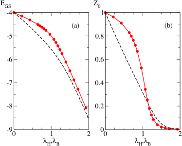
Figure 1: (color online) (a) GS energy and (b) GS $qp$ weight as a function of the corresponding dimensionless coupling parameter. The dashed line corresponds to the Holstein model, while the breathing-mode results are shown by circles (line is a guide to the eye). Parameters are $t=2,\Omega=1$.

The ground state energy $E_{GS}$ and quasiparticle ($qp$) weight $Z_{0}=|\langle\Phi_{GS}|c^{\dagger}_{k=0}|0\rangle|^{2}$, where $|\Phi_{GS}\rangle$ is the ground-state eigenfunction, are shown in Fig. 1 for the 1D breathing-mode and Holstein models. For a fixed value of $\alpha$, we see the expected crossover from a large polaron (at weak coupling $\lambda_{B,H}$) to a small polaron (at strong coupling $\lambda_{B,H}$), signaled by the collapse of the $qp$ weight.

The ground state energy of both models decreases monotonically with increasing coupling, but that of the Holstein polaron is lower. This is in agreement with the second order strong-coupling perturbation results in Eq. (11) and (12). Unlike the rather gradual decrease in the quasiparticle weight of the 1D Holstein polaron, the 1D breathing-mode polaron shows a large $Z_{0}$ at weak couplings, followed by a much sharper collapse at the crossover near $\lambda_{B}\approx 1$. The reason for the enhanced $Z_{0}$ at weak couplings is straightforward to understand. Here, the wave-function is well described by a superposition of the free electron and electron-plus-one-phonon states. Given the conservation of the total polaron momentum $K=0=k+q$ and the large electron bandwidth $t$, states with high electron and phonon momenta have high energies and thus contribute little to the weak-coupling polaron ground-state. On the other hand, the coupling $g(q)\sim\sin(q/2)$ to the low-energy states with low electron and phonon momenta is very small for the breathing-mode model. This explains the slower transfer of spectral weight at weak coupling for breathing-mode versus the Holstein polaron.

The energy (measured from $E_{GS}$) and $qp$ weight of the first excited $K=0$ state are shown in Fig. 2. For both models, at weak-coupling this state is precisely at $\Omega$ above the ground-state energy, at the lower edge of the polaron+one-phonon continuum. As the coupling increases above a critical value, a second bound state gets pushed below the continuum. This second bound state is absent in SCBA calculations.scba The separation between the two lowest energy states now first decreases and then increases back towards $\Omega$ as $\lambda_{H,B}\rightarrow\infty$. This behavior is well-known for the Holstein polaron.bonca The breathing-mode polaron shows the same qualitative behavior. Note that below the critical coupling, the computed energy of the first excited state is slightly larger than $\Omega$. The reason is a systematic error that can be reduced by increasing the number of one-phonon basis states, in order to better simulate the delocalized phonon that appears in this state. The $qp$ weight of the first excited state is zero below the critical coupling, due to the crossing between on-site and off-site phonon states.bonca

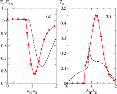
Figure 2: (color online) (a) Energy of the first excited $K=0$ state, measured from $E_{GS}$, and (b) its $qp$ weight. The dashed line corresponds to the Holstein model, while the breathing-mode results are shown by circles (line is a guide to the eye). Parameters are $t=2,\Omega=1$.

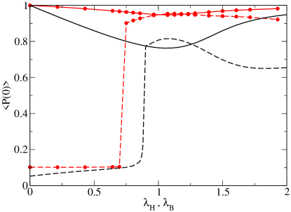
Figure 3: (color online) P(0) for $t=2,\Omega=1$ for the breathing-mode (red symbols) and Holstein (black line) models, respectively. The solid and dashed lines correspond to ground state and first excited state, respectively.

The nature of the these states is revealed by checking the locality of the phonon cloud. We define the projection operator

$$P(K)=\sum_{S_{local}}|S,K\rangle\langle S,K|$$

where the summation is over all states with $m_{H}=0$ and $m_{B}=\pm 0.5$ in Eq. (13). Comparison with Eq. (14) shows that this operator selects only basis states with phonons only on the electron site (Holstein) and only on the two phonon sites bracketing the electron site (breathing-mode). Fig. 3 shows the expectation value of this operator for the two lowest eigenstates of both models. For both ground-states $\langle P(0)\rangle\sim 1$, indicating that here most phonons are neariest to the electron. However, at weak coupling the first excited state (which is here the band-edge of the polaron + free phonon continuum) has $\langle P(0)\rangle\rightarrow 0$, precisely because the free phonon can be anywhere in the system. When the second bound states form, $\langle P(0)\rangle$ becomes large, showing that phonons in these states are primarily localized near the electron.bonca While there appears to be a crossing between the ground-state and first-excited state values, we emphasize that $P(K)$ measures the locality of the phonon cloud, not its structure.

Table 2: $\alpha_{n_{-},n_{+}}$ vs. $n_{+},n_{-}$ for the ground state

$t=2$ $\Omega=1$ $g=0$ $\Delta=0$ $n_{+}n_{-}$ $0$ $1$ $2$ $3$ 0 1.0000 0.0000 0.0000 0.0000 1 0.0000 0.0000 0.0000 0.0000 2 0.0000 0.0000 0.0000 0.0000 3 0.0000 0.0000 0.0000 0.0000 $t=2$ $\Omega=1$ $g=1.5$ $\Delta=1.05$ $n_{+}n_{-}$ $0$ $1$ $2$ $3$ 0 0.9150 0.0584 0.1372 -0.0477 1 -0.0584 -0.1681 0.0520 -0.0536 2 0.1372 -0.0520 0.0549 -0.3300 3 0.0477 -0.0536 0.0330 -0.0255 $t=2$ $\Omega=1$ $g=1.964$ $\Delta=1.964$ $n_{+}n_{-}$ $0$ $1$ $2$ $3$ 0 0.9876 -0.0509 0.0082 -0.0025 1 0.0509 -0.0100 0.0034 -0.0020 2 0.0082 -0.0034 0.0022 -0.0019 3 0.0025 -0.0020 0.0019 -0.0019

For the breathing-mode model, these results suggest the possibility to describe them using the on-site coherent-state structure. That is, a Lang-Firsov state with $n_{-}$ and $n_{+}$ number of phonons excited to the left and right of the electron site, mapped to real space by Eq. (14). We note that we are no longer in the strong coupling regime and the transformation cannot be determined by $g$ and $\Omega$ alone, therefore we seek an effective transformation with

$$\tilde{S}(\Delta)=S_{B}|_{\frac{g}{\Omega}=\Delta}$$

The computed eigenstates $|\phi\rangle$ are projected into such structure $\alpha_{n_{-},n_{+}}$ by

$$\frac{1}{\sqrt{N}}\sum_{l}e^{iKl}c_{l}^{\dagger}\sum_{n_{-},n_{+}=1}^{\infty}\alpha_{n_{-},n_{+}}\frac{(b_{l-{1\over 2}}^{\dagger})^{n_{-}}}{\sqrt{n_{-}!}}\frac{(b_{l+{1\over 2}}^{\dagger})^{n_{+}}}{\sqrt{n_{+}!}}|0\rangle$$

$$=e^{\tilde{S}(\Delta)}P(K)|\phi\rangle$$

Table 3: $\alpha_{n_{-},n_{+}}$ vs. $n_{+},n_{-}$ for the first-excited state

$t=2$ $\Omega=1$ $g=1.5$ $\Delta=1.05$ $n_{+}n_{-}$ $0$ $1$ $2$ $3$ 0 0.0228 -0.6515 0.0152 0.1151 1 0.6515 0.0062 0.1700 -0.0473 2 0.0152 -0.1700 0.0505 -0.0456 3 0.1151 -0.0473 0.0456 -0.0220 $t=2$ $\Omega=1$ $g=1.964$ $\Delta=1.964$ $n_{+}n_{-}$ $0$ $1$ $2$ $3$ 0 -0.0859 -0.6675 0.0630 -0.0164 1 0.6675 -0.0864 0.0246 -0.0120 2 0.0630 -0.0246 0.0134 -0.0099 3 0.0164 -0.0120 0.0099 -0.0089

Table  2 and 3 show the results of such projections for the ground state and for the first excited bound state. It is clear that they can be rather well described as $|GS\rangle\sim e^{-\tilde{S}(t,g,\Omega,K)}\frac{1}{\sqrt{N}}\sum_{l}e^{iKl}c_{l}^{\dagger}|0\rangle$, respectively $|1\rangle_{\rm bound}\sim e^{-\tilde{S}(t,g,\Omega,K)}\frac{1}{\sqrt{N}}\sum_{l}e^{iKl}c_{l}^{\dagger}(e^{i\theta}b_{l-{1\over 2}}^{\dagger}-e^{-i\theta}b_{l+{1\over 2}}^{\dagger})|0\rangle$ for some phase $\theta(t,g,\Omega,K)$ needed to satisfy time-reversal symmetry. These states no longer have definite parity symmetry like those of the Holstein model. The symmetry is broken by the anti-symmetric coupling term in the model. If the free-electron component is non-zero for an eigenstate, its components with odd/even number of phonons should have odd/even parity. For increasing momentum, this description is valid as long as the excited state remains bound, with energy less than $E_{GS}+\Omega$.

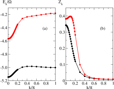
Figure 4: (color online) The $k$-dependent (a) energy and (b) $qp$ weight of the GS (circles) and first bound state (square) for the 1D breathing mode model, for $t=2,\Omega=1,\lambda_{B}=1.07$.

Fig. 4 shows momentum dependent energy and $qp$ weight for the two lowest eigenstates of the breathing-mode model, for an intermediate coupling strength $\lambda_{B}=1.07$. The polaron band has a maximum at $k\sim 0.4\pi$, in qualitative agreement with the strong-coupling perturbation theory results. This behavior is not captured by SCBA which is only accurate for low coupling strength.scba For the Holstein polaron, the polaron dispersion is a monotonic function of momentum.bonca Even though the $qp$ weights remain moderately high at zero momentum, the weights collapse towards zero with increasing momentum, similar to the well-known Holstein case. This is due to the fact that at large total momentum, the significant contribution to the eigenstate comes from states with at least one or more phonons. The free electron state has a large energy for large momentum, and contributes very little to the lowest energy eigenstates, so indeed $Z\rightarrow 0$.

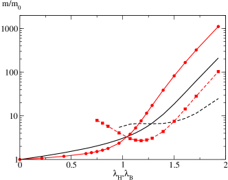
Figure 5: (color online) Ratio of effective polaron mass to that of the free electron. Circles and squares show breathing-mode results for GS and first bound state, respectively. The other lines correspond to the Holstein model GS (full) and second bound state (dashed). Parameters are $t=2,\Omega=1$.

The effective masses for the two lowest eigenstates of both models are shown in Fig. 5, as a function of $\lambda_{H,B}$. These were calculated from the second derivative of the energy at momentum $K=0$. For the GS of both models, the effective mass increases monotonically with $\lambda_{H,B}$. At weak couplings, the breathing-mode polaron is lighter than the Holstein polaron. As already discussed, this is due to the vanishingly weak coupling to low-momentum phonons. At strong coupling, however, the effective mass is larger for the breathing-mode polaron. This is in agreement with predictions of the strong-coupling perturbation theory, and results from the fact that the hopping of a breathing-mode polaron involves phonon clouds on $2z-1$ phonon sites, whereas hopping of a Holstein polaron involves phonons at only two sites.

The effective mass of the first excited state can only be defined once this state has split-off from the continuum. It has non-monotonic behavior, first decreasing and then increasing with increasing $\lambda_{H,B}$. This can be understood through the link of the effective mass and the $qp$ weight. In terms of derivatives of the self-energy $\Sigma(k,\omega)$, the effective mass $m^{*}$ is given by:

$${m^{*}\over m}=\left(1-\frac{\partial\Sigma}{\partial\omega}\right)\cdot\left(1+{m\over\hbar^{2}}\frac{\partial^{2}\Sigma}{\partial k^{2}}\right)^{-1},$$

where derivatives are evaluated at $K=0$ and at the corresponding eigenenergy. The first term is linked to the $qp$ weight, $Z=(1-\frac{\partial\Sigma}{\partial\omega})^{-1}$, so that $m^{*}\sim 1/Z$. As shown in Fig. 2(b), the $qp$ weight of the first excited state has non-monotonic behavior, leading to the non-monotonic behavior of the effective mass.

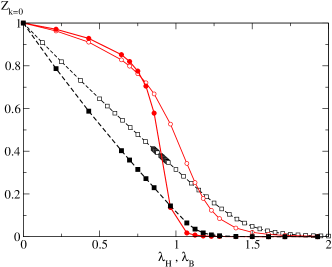
Figure 6: (color online) GS $qp$ weights for the breathing-mode (circles) and Holstein (squares) models. Full symbols correspond to $\alpha=8$. For comparison purposes, the empty symbols show the $\alpha=4$ results of Fig. 1(b). ($\Omega=1$)

All the results shown so far were for $\alpha=4$. For higher $\alpha$ (lower $\Omega$ and/or larger $t$), the difference between the two models can be grasped from Fig. 6. Similar to the Holstein model, the large-to-small polaron transition occurs at lower $\lambda$ for increasing $\alpha$.v6 ; a2 At weak and moderate coupling, the $qp$ weight and the effective mass (not shown) in the breathing-mode model are much less sensitive to an increase in $\alpha$, than is the case for the Holstein polaron. This suggests that breathing-mode polarons should be better charge carriers than the Holstein polarons, in this regime.

III.2 Spectral Function

Figure 7: The spectral function of the 1D breathing-mode model, on linear (left) and logarithmic (right) scales. The curves are shifted for better viewing, and correspond (top to bottom) to $\lambda_{B}=1.5;1.25;1.0$ and $0.75$. Vertical lines indicates $E_{GS}$ and $E_{GS}+\Omega$. $K=0,t=2,\Omega=1,\eta=0.004\Omega$.

The spectral function is proportional to the imaginary part of the Green’s function:

$$A(k,\omega)=-\frac{1}{\pi}\mbox{Im}G(k,\omega)$$ (16)

In terms of single electron eigenstates and eigenfunction $H|n\rangle=E_{n}|n\rangle$, we obtain the Lehmann representation:

$$A(k,\omega)=\sum_{n}|\langle n|c^{{\dagger}}_{k}|0\rangle|^{2}\delta(\omega-E_{n})$$

Of course, since we use a finite small $\eta$ in numerical calculations, the $\delta$-functions are replaced Lorentzians of width $\eta$ [see Eq. (15)]. We calculate the Green’s functions as discussed in the previous section.

Fig. 7 shows the spectral function for zero momentum as a function of energy. Results corresponding to four different coupling strengths $\lambda_{B}$ from near the crossover region are shown for the breathing-mode polaron. We note that there is always a continuum starting at one phonon quantum above the ground state energy. This is more clearly visible in the right panel, where the spectral weight is shown on a logarithmic scale, and vertical lines mark the position of the ground-state energy $E_{GS}$, respectively of $E_{GS}+\Omega$. As the coupling $\lambda_{B}$ increases, we see the appearance of the second bound state below the continuum. We only find at most one extra bound state in this energy range for all coupling strengths. As $\lambda_{B}$ increases, the spectral weight of the first continuum decreases dramatically. Other bound states form above it, followed by higher energy continua whose weight is also systematically suppressed. This is qualitatively similar to the behavior exhibited by Holstein polaron.a3

Figure 8: $A(k,\omega)$ vs $\omega$, for $K/\pi$=0; 0.25; 0.5; 0.75 and 1 (top to bottom) for intermediate coupling $t=2,\Omega=1,\lambda_{B}=1.25$. $\eta/4=\Delta E=0.001\Omega$. The height of the spectral weight is plotted in linear scale on the left and logarithmic scale on the right. The two vertical lines indicate $E_{GS}$ and $E_{GS}+\Omega$.

Fig. 8 illustrates the momentum dependence of the breathing-mode polaron’s spectral weight. The results correspond to a coupling above the critical value, where there is a second bound state. The majority of the spectral weight is transferred to much higher energies as the momentum increases, and a broad feature develops at roughly the position of the free-electron energy for that momentum. This spectral weight transfer is also qualitatively similar to what is observed for Holstein polarons. Our results have a high-enough resolution to clearly show the continuum at $E_{GS}+\Omega$ for all values of $K$. This is part of the kink-like structure reported in Ref. scba, . The logarithmic plot clearly reveals a non-monotonic dispersion of the ground-state like in Fig. 4, characteristic for the breathing-mode polaron.

Fig. 8 shows only one peak located between the ground-state and the polaron+one-phonon continuum, even though in fact we believe that there are more than one eigenstates within this region. We found, from eigenvalue computation, additional energy states below the continuum; however, computation of exact energy values requires prohibitively long compution time due to the clustering of eigenvalues. By observing the convergence behavior due to increasing basis size, we can conclude that additional bound states do exist below the continuum. The lack of their contribution to the spectral function can be understood by the fact that the single particle Green’s function only contains information about eigenstates with finite $qp$ weight, $|\langle\phi|c_{K}^{\dagger}|0\rangle|^{2}>0$, see Eq. (15). These eigenstates must have components corresponding to some Lang-Firsov eigenstate with no off-site phonons (Eq. (14)). Also, the wave-function of these states must have a peculiar space inversion symmetry: S-symmetric for all even-phonon-number components and P-symmetric for all odd-phonon-number components. The ground-state always satisfies this requirement, but above a critical coupling, only one other state below the phonon threshold satisfies this requirement.

IV Conclusions

In summary, we have reported here the first accurate numerical study of the 1D breathing-mode polaron. A previous studyscba based on the self-consistent Born approximation proves to be inadequate to describe correctly the behavior for medium and strong couplings, as expected on general grounds.

Comparison with the Holstein model results, which correspond to a coupling $g(q)=const.$, reveals some of the similarities and differences of the two models. The breathing-mode polaron is much more robust (has a much larger $qp$ weight, and less variation with parameters) at weak couplings. This is a direct consequence of the fact that coupling to low-momentum phonons, which is relevant here, becomes vanishingly small $g(q)\sim\sin(q/2)\rightarrow 0$. Similar behavior is expected for any other $g(q)$ model if $\lim_{q\rightarrow 0}g(q)\rightarrow 0$. On the other hand, at strong couplings the breathing-mode polaron is much heavier and has a lower $qp$ weight than the Holstein polaron. This also results from strong-coupling perturbation results, and is due to the fact that in order to move from site $i$ to site $i+1$, a small breathing-mode polaron must (i) create a new polaron cloud at site $i+\frac{3}{2}$; (ii) rearrange the polaron cloud at site $i+{1\over 2}$, so that its displacement is now pointing towards site $i+1$, not towards site $i$; and (iii) relax (remove) the phonon cloud at site $i-{1\over 2}$. This results in a suppressed polaron kinetic energy, and an enhanced effective mass. Because of the larger $Z$ at weak coupling, and the lower $Z$ at strong couplings, the crossover from large to small polaron is much sharper for the breathing-mode polaron. Another interesting observation is that the polaron dispersion becomes non-monotonic with momentum $k$ for medium and large couplings. This can be understood in terms of strong-coupling perturbation theory, which shows that the second-order $\cos(2k)$ correction is larger than the first-order $\cos(k)$ correction for large-enough couplings.

Similarities with the Holstein behavior regard the appearance of the polaron+free phonon continuum at $E_{GS}+\Omega$, and the appearance of a second bound state with finite $qp$ weight for large-enough couplings. The convergence of numerics points to the existence of additional bound states, whose absence from the spectral function can be explained by symmetry or missing free-electron componenets in the wavefunction; however, this issue is not fully settled. Also, the importance of such states for the physical properties is not known. The general aspect of the higher energy spectral weight at strong couplings, as a succession of bound states with large spectral weight and continua with less and less spectral weight, is also reminiscent of the Holstein polaron results.

Acknowledgments: We thank Jeremy Heyl for giving us permission to use his cluster. This work was supported by CFI (access to the clusters yew, westgrid and jmd), by NSERC, and by CIfAR Nanoelectronics and the Alfred P. Sloan Foundation (M.B.) and CIAR Quantum Materials (G.S.).

References

- (1) M. B. Salamon and M. Jaime, Rev. Mod. Phys. 73, 583 (2001).
- (2) K. M. Shen, F. Ronning, D. H. Lu, W. S. Lee, N. J. C. Ingle, W. Meevasana, F. Baumberger, A. Damascelli, N. P. Armitage, L. L. Miller, Y. Kohsaka, M. Azuma, M. Takano, H. Takagi, and Z.-X. Shen, Phys. Rev. Lett. 93, 267002 (2004).
- (3) T. Cuk, D. H. Lu, X. J. Zhou, Z.-X. Shen, T. P. Devereaux, N. Nagaosa, Phys. Stat. Sol. (b) 242, 1 (2005)
- (4) T. Holstein, Ann. Phys. (N.Y.) 8, 325 (1959).
- (5) F. Marsiglio, Phys. Rev. B 42, 2416 (1990).
- (6) H. DeRaedt and A. Lagendijk, Phys. Rev. Lett. 49, 1522 (1982).
- (7) H. DeRaedt, A. Lagendijk, Phys. Rev. B 27, 6097 (1983).
- (8) H. DeRaedt, A. Lagendijk, Phys. Rev. B 30, 1671 (1984).
- (9) P. Kornilovitch, J. Phys.: Condens. Matter 9, 10675 (1997).
- (10) P. E. Kornilovitch and E. R. Pike, Phys. Rev. B 55, R8634 (1997).
- (11) P. E. Kornilovitch, Phys. Rev. B 60, 3237 (1999).
- (12) P. E. Kornilovitch, Phys. Rev. Lett. 81, 5382 (1998).
- (13) M. Hohenadler, H. G. Evertz, and W. von der Linden, Phys. Status Solidi B 242, 1406 (2005).
- (14) M. Hohenadler, H. G. Evertz, and W. von der Linden, Phys. Rev. B 69, 024301 (2004).
- (15) N. V. Prokof’ev and B. V. Svistunov, Phys. Rev. Lett. 81, 2514 (1998).
- (16) A. Macridin, Ph.D. thesis, University of Groningen, http:// irs.ub.rug.nl/ppn/25013585X (2003).
- (17) J. Bonca, S. A. Trugman, I. Batistic, Phys. Rev. B 60, 1633 (1999).
- (18) A. H. Romero, D. W. Brown, and K. Lindenberg, Phys. Rev. B 59, 13728 (1999).
- (19) A. H. Romero, D. W. Brown, K. Lindenberg, Phys. Rev. B 60, 4618 (1999).
- (20) A. H. Romero, D. W. Brown, K. Lindenberg, Phys. Rev. B 60, 14080 (1999).
- (21) V. Cataudella, G. De Filippis, and G. Iadonisi, Phys. Rev. B 60, 15163 (1999).
- (22) V. Cataudella, G. De Filippis, and G. Iadonisi, Phys. Rev. B 62, 1496 (2000).
- (23) Li-Chung Ku, S. A. Trugman, and J. Bonca, Phys. Rev. B 65, 174306 (2002).
- (24) V. Cataudella, G. De Filippis, F. Martone, and C. A. Perroni, Phys. Rev. B 70, 193105 (2004).
- (25) G. De Filippis, V. Cataudella, V. Marigliano Ramaglia, and C. A. Perroni, Phys. Rev. B 72, 014307 (2005).
- (26) O. S. Barisic, Phys. Rev. B 65, 144301 (2002).
- (27) O. S. Barisic, Phys. Rev. B 69, 064302 (2004).
- (28) F. Marsiglio, Phys. Rev. B 42, 2416 (1990).
- (29) G. Wellein and H. Fehske, Phys. Rev. B 58, 6208 (1998).
- (30) A. S. Alexandrov, V. V. Kabanov, and D. K. Ray, Phys. Rev. B 49, 9915 (1994).
- (31) G. Wellein, H. R der, and H. Fehske, Phys. Rev. B 53, 9666 (1996).
- (32) G. Wellein and H. Fehske, Phys. Rev. B 56, 4513 (1997).
- (33) E. V. L. de Mello and J. Ranninger, Phys. Rev. B 55, 14872 (1997).
- (34) M. Capone, W. Stephan, and M. Grilli, Phys. Rev. B 56, 4484 (1997).
- (35) F. Marsiglio, Physica C 244, 21 (1995).
- (36) P. E. Kornilovitch, Euro. phys. Lett. 59, 735 (2002).
- (37) M. Berciu, PRL 97, 036402 (2006).
- (38) G. L. Goodvin, M. Berciu, G. A. Sawatzky, Phys. Rev. B 74, 245104 (2006).
- (39) M. Berciu and G. L. Goodvin, arXiv:0705.4154.
- (40) F. C. Zhang and T. M. Rice, Phys. Rev. B 37, 3759 (1988).
- (41) K. J. Szczepanski, K. W. Becker, Z. Phys. B 89, 327 (1992).
- (42) O. Rosch, O. Gunnarsson, Phys. Rev. Lett. 92, 146403 (2004).
- (43) D. Poilblanc, T. Sakai, D. J. Scalapino, W. Hanke, Europhys. Lett., 34 367 (1996).
- (44) C. Slezak, A. Macridin, G. A. Sawatzky, M. Jarrell, T. A. Maier, Phys. Rev. B 73 205122 (2006).
- (45) R.B. Lehoucq, D.C. Sorensen, C. Yang , ARPACK Users’ Guide: Solution of Large-scale Eigenvalue Problems with Implicitly Restarted Arnoldi Methods (SIAM, US, 1998).
- (46) We have reported a software bug in the parallel version of the ARPACK package, but the package has not been updated as of to date.
- (47) G. D. Mahan, Many-Particle Physics, (Plenum, New York, 1981).
- (48) E. Dagotto, Rev. Mod. Phys. 66, 3 (1994)
- (49) J. W. Demmel, Applied Numerical Linear Algebra, (SIAM, US, 1981).
- (50) H. Simon, Math. Comp. 42, 165 (1984).