Isolating Triggered Star Formation

Abstract

Galaxy pairs provide a potentially powerful means of studying triggered star formation from galaxy interactions. We use a large cosmological N-body simulation coupled with a well-tested semi-analytic substructure model to demonstrate that the majority of galaxies in close pairs reside within cluster or group-size halos and therefore represent a biased population, poorly suited for direct comparison to “field” galaxies. Thus, the frequent observation that some types of galaxies in pairs have redder colors than “field” galaxies is primarily a selection effect. We use our simulations to devise a means to select galaxy pairs that are isolated in their dark matter halos with respect to other massive subhalos (N$=2$ halos) and to select a control sample of isolated galaxies (N$=1$ halos) for comparison. We then apply these selection criteria to a volume-limited subset of the 2dF Galaxy Redshift Survey with M${}_{\rm B,j}\leq-19$ and obtain the first clean measure of the typical fraction of galaxies affected by triggered star formation and the average elevation in the star formation rate. We find that 24% (30.5 %) of these L^⋆ and sub-L^⋆ galaxies in isolated 50 (30) h^-1 kpc pairs exhibit star formation that is boosted by a factor of $\gtrsim 5$ above their average past value, while only 10% of isolated galaxies in the control sample show this level of enhancement. Thus, 14% (20 %) of the galaxies in these close pairs show clear triggered star formation. Our orbit models suggest that 12% (16%) of 50 (30) h^-1 kpc close pairs that are isolated according to our definition have had a close ($\leq$ 30 h^-1 kpc) pass within the last Gyr. Thus, the data are broadly consistent with a scenario in which most or all close passes of isolated pairs result in triggered star formation. The isolation criteria we develop provide a means to constrain star formation and feedback prescriptions in hydrodynamic simulations and a very general method of understanding the importance of triggered star formation in a cosmological context.

1. Introduction

Galaxy interactions and mergers help drive galaxy evolution. In the concordance $\Lambda$CDM cosmological model, nearly every galaxy has had a major merger at least once over cosmic time (e.g., Maller et al., 2006; Stewart et al., 2007). Major mergers and interactions consume available gas, producing stellar populations which subsequently redden with age (e.g., Larson & Tinsley, 1978; Kennicutt et al., 1987). Major mergers destroy disks, turning galaxies into spheroids (e.g., Toomre & Toomre, 1972), but also potentially creating large disk galaxies in gas-rich scenarios (e.g., Robertson et al., 2006). Close galaxy passes and minor mergers are even more frequent. These perturbations send gas into the centers of galaxies, where they may contribute to bulge components and even feed black holes (e.g., Kennicutt & Keel, 1984; Barnes & Hernquist, 1992; Mihos & Hernquist, 1996; Barton et al., 2000; Combes, 2001; Barton et al., 2001; Barton Gillespie et al., 2003; Kannappan, Jansen, & Barton, 2004; Kormendy & Kennicutt, 2004; Freedman Woods, Geller, & Barton, 2006; Lin et al., 2007; Alonso et al., 2007; Freedman Woods & Geller, 2007). In the hierarchical picture of galaxy formation, mergers play an even more important role during earlier epochs than they do today, possibly triggering the high star formation rates (Lowenthal et al., 1997; Kolatt et al., 1999; Somerville et al., 2001; Wechsler et al., 2001) observed in some “Lyman break” galaxies at $z\gtrsim 3$ (Steidel & Hamilton, 1992; Steidel et al., 1996) or luminous submillimeter galaxies (e.g., Chapman et al., 2005).

Existing detailed studies of galaxy interactions show that triggered star formation and morphological evolution can be very rapid and intense. However, we can only observe a “snapshot” of the evolution of galaxy pairs. With incomplete phase-space information, we do not know their true frequency, evolutionary timescales, orbits, or fates. Thus, we have neither a complete understanding of the frequency of interactions and mergers nor knowledge of their impact on galaxy evolution. Many processes such as ram pressure stripping, interaction with a cluster or group potential, or high-speed “harassment,” may also be very important in establishing the morphologies and stellar populations of galaxies, and in driving the relationships between morphology, color, and local environmental density (e.g., Gunn & Gott, 1972; Dressler, 1980; Postman & Geller, 1984; Moore et al., 1996; Blanton et al., 2005a).

Hydrodynamic simulations of galaxy interactions can make predictions for the expected star formation rate from any type of galactic collision (e.g., Barnes & Hernquist, 1992; Mihos & Hernquist, 1996; Springel, Di Matteo, & Hernquist, 2005; Cox et al., 2006; Perez et al., 2006a, b). However, these predictions are sensitive to prescriptions for baryonic physics that are highly uncertain. In particular, hydrodynamic simulations must rely on effective models for gas dynamics, cooling, and star formation that these simulations cannot hope to resolve. Uncertainties in these effective theories are an enormous problem for galaxy formation theory and detailed tests of these prescriptions are required. Unfortunately such tests are not simple; the full phase-space information is not known for many real systems. However, empirical, statistical studies of galaxy interactions and mergers — when combined with predictions of galaxy orbits in a now well-established cosmological model — hold promise for uncovering the role of interactions and mergers in galaxy evolution.

The first step in studying the effects of interactions and mergers is to identify systems that are undergoing these processes. Using morphological distortion as an indicator of galaxy interactions does yield a subset of the pairs that have definitely had a close pass. However, relying on tidal distortion leads to missed interacting pairs because (1) sensitivity to low-surface-brightness features is a strong function of seeing, depth, and redshift, (2) the morphological features are short-lived ($\sim$100 Myr), and (3) many of the features, like tidal tails, are resonance effects that only appear in prograde disk galaxy encounters (Toomre & Toomre, 1972). For a more complete census of the effects of interactions, it is important to select pairs or systems of galaxies based only on proximity in redshift and projected separation, then to use mock catalogs constructed from cosmological simulations to understand this selection.

Historically, studies of distorted galaxies and galaxies in pairs have been very revealing. The early stages of galaxy interactions can drive gas into the center of a progenitor galaxy and trigger an early episode of central star formation long before the final merger (e.g., Larson & Tinsley, 1978; Joseph et al., 1984; Kennicutt et al., 1987; Mihos & Hernquist, 1994, 1996). The strength of the optical emission line associated with this star formation correlates with the separation of the pair on the sky ($\Delta D$) and in redshift ($\Delta V$; Barton et al., 2000). The optically-detected star formation is strongest in the central few kpc, often dominating the optical light; in the case of a late-type spiral, it can also contribute substantially to the formation of a bulge (Tissera et al., 2002; Barton Gillespie et al., 2003). This process may be the primary mechanism for the formation of late-type bulges (Kannappan, Jansen, & Barton, 2004). Kewley et al. (2006) show that the metallicities of these galaxies provide a “smoking gun” for gas infall from the outskirts of the disks. Galaxies with (optically) strong central starbursts have metallicities that are lower than average for their luminosities, consistent with a starburst occurring in gas that was driven into the nucleus from the metal poor outskirts of the progenitor’s disk.

New, large redshift surveys such as the 2dFGRS (Colless et al., 2001) and Sloan Digital Sky Survey (York et al., 2000) provide a means of exploring ever-larger samples of galaxies in pairs, although these samples must be approached with caution because mechanical spectrograph constraints make them deficient in close pairs. The correlations between orbital parameters and star-forming properties of galaxies in pairs have been verified in both the 2dFGRS (Lambas et al., 2003), and the SDSS (Nikolic et al., 2004; Luo et al., 2007). However, the studies also appear to reveal unexpected phenomena including apparently suppressed star formation in widely-separated pairs and red tails in the color distributions of paired galaxies (Lambas et al., 2003; Alonso et al., 2004, 2006; Luo et al., 2007).

Using these empirical results to arrive at a true measure of the amount and timescales of triggered star formation is difficult. Pair samples are complex: they include some interlopers and are rich in galaxies in a variety of environments (e.g., Alonso et al., 2006; Soares, 2007). The progenitors of galaxy interactions come from a mixture of galaxy types (e.g., Focardi et al., 2006). In dense environments, many will have already experienced multiple close passes and mergers. They may have consumed or lost much of their gas, leaving little to form new stars. However, in sparser environments, the progenitors of the interaction may have had very few previous interactions. They may have large remaining gas reservoirs. Thus, the efficacy of an interaction in triggering star formation should depend in detail on the environment of the interacting galaxies.

Dense clusters of galaxies are straightforward to identify with confidence. However, the low-speed encounters that trigger star formation are extremely unlikely in these clusters. An understanding of tidally-triggered star formation requires accurate probes of isolated galaxies and sparse loose groups. Unfortunately, accurate environmental statistics are difficult to interpret precisely in this regime. Group-finding algorithms are effective at investigating environments (Huchra & Geller, 1982). However, even highly tuned group-finding algorithms construct false groups and miss group members (e.g., Yang et al., 2005; Gerke et al., 2005; Weinmann et al., 2006; Berlind et al., 2006; Koester et al., 2007). Nearest-neighbor and counts-in-cylinder statistics also have a large scatter (e.g., Berrier et al., 2007).

The use of mock galaxy catalogs based on numerical simulations of structure formation in the standard cosmology can help sort these issues out. Direct numerical simulation is difficult because obtaining the necessary resolution to be complete in close pairs while simultaneously modeling a large enough volume to reduce sample variance is computationally expensive. An alternative and proven method is to use an analytic model for dark matter halo substructure (so-called “subhalos”, e.g., Zentner & Bullock, 2003; Taylor & Babul, 2004; Zentner et al., 2005) in conjunction with an $N$-body simulation of a cosmologically-relevant volume. The analytic model treats halo substructure using a method that is approximate, but free of inherent resolution limits, and extends the effective numerical resolution in the simulated volume, ensuring completeness in the dense environments where many close pairs reside. The analytic model also allows for a quantification of shot-noise contributions to close-pair samples that may arise, for example, from the particulars of galaxy orbits and may be significant (Berrier et al., 2006). Such models have been developed and validated by comparison to direct $N$-body simulations in the regimes where the two techniques are commensurable (Zentner et al., 2005). Thus, the time is ripe to develop new methods aimed at understanding the detailed make-up of pairs of galaxies selected from redshift surveys.

We study mock catalogs constructed using the hybrid approach described briefly in the previous paragraph and extensively in Zentner et al. (2005) and Berrier et al. (2006). This approach has already succeeded in explaining the apparent lack of evolution in the close pair fraction observed in intermediate-redshift surveys (Lin et al., 2004; Berrier et al., 2006). In the present study, we focus on interpreting the star-forming properties of galaxies in pairs. With the complexities of the large-scale environments of pairs in mind, we explore the construction of appropriate samples and control samples for galaxies in pairs. In particular, we examine ways to isolate the immediate effects of triggered star formation from other environmental processes. Here, we apply the analysis to a volume-limited sample of galaxies in the 2dFGRS; however, the techniques we discuss are generally applicable to other studies of tight sub-groupings of galaxies.

In § 2 we describe the numerical methods and the observational data that we use. § 3 contains a description of the model predictions for the environments of galaxies in pairs; in this section we examine the problem of trying to construct a control sample of objects that are not in pairs. In § 4, we restrict to the most isolated pairs and individual galaxies and show that isolated pairs are almost purely dark matter halos containing N $=2$ galaxies inside their virial radii. The isolated galaxies we select are an appropriate control sample for the progenitors of an interaction. We examine galaxies in pairs in the 2dF Galaxy Redshift Survey (2dFGRS Colless et al., 2001) in § 5 and measure the amount of triggered star formation in isolated pairs relative to the control. We § 7 contains a brief description of the situation in more complex environments, and we conclude in § 8. In future papers, we plan to explore more complex environments in greater detail. The ultimate goal of this and similar studies is to isolate the effects of interactions and then re-integrate the results into a complete cosmological interaction history for galaxies, thus measuring the amount of galaxy evolution triggered by interactions and mergers.

2. The Models and the Data

The first step in our study is to construct mock catalogs of galaxies and study the environments of galaxies in projected, close-pair configurations in order to understand the selection of such objects. We use the information gleaned from the mock samples to aid in the interpretation of close pairs in the 2dFGRS. In this section, we describe the models used to produce mock catalogs and the observational data in turn.

2.1. Mock Galaxy Catalogs

Our model begins with a cosmological N-body simulation from which we extract positions and masses of host dark matter halos within a cosmological volume. We populate the host halos with subhalos using the method of Zentner et al. (2005). Our method for producing mock catalogs has been discussed in detail in Berrier et al. (2006). We provide a brief overview here, and refer the reader to Berrier et al. (2006) for a more detailed discussion.

Our numerical simulation was run with the Adaptive Refinement Tree N-body code (Kravtsov et al., 1997) in a standard $\Lambda$CDM cosmology with $\Omega_{m}=0.3$, $\Omega_{\Lambda}=0.7$, H₀ = 70 km s^-1 Mpc^-1, and $\sigma_{8}=0.9$. The simulation followed the evolution of $512^{3}$ particles in comoving box of $120$ h^-1 Mpc on a side, implying a particle mass of $m_{p}\simeq 1.1\times 10^{9}$ h ${}^{-1}M_{\odot}$. The simulation grid was refined down to a minimum cell size of $h_{\mathrm{peak}}\simeq 1.8$ h^-1 kpc on a side. The simulation was previously discussed in Tasitsiomi et al. (2004), Zentner et al. (2005), Allgood et al. (2006), and Wechsler et al. (2006). Host halos in the simulation were identified using a variant of the Bound Density Maxima algorithm (BDM, Klypin et al., 1999; Kravtsov et al., 2004). We define a halo virial radius as the radius of the sphere, centered on the density peak, within which the mean density is $\Delta_{v}(z)$ times the mean density of the universe, $\rho_{m}$. The virial overdensity $\Delta_{v}(z)$, is given by the spherical top-hat collapse approximation and we compute it using the fitting function of Bryan & Norman (1998). Host halos are identified as those halos whose centers do not lie within the virial radius of another halo.

In order to determine the substructure properties in each host dark matter halo, we model their mass accretion histories and track their substructure content using an analytic technique that exploits numerous simplifying approximations and several scaling relations derived from direct simulation (Zentner et al., 2005). For each host halo of mass $M$ at redshift $z$ in our simulation volume, we randomly generate a mass accretion history using the method of Somerville & Kolatt (1999). At each merger event, we assign an initial orbital energy and angular momentum to the infalling object according to the probability distributions for these quantities derived from cosmological $N$-body simulations (Zentner et al., 2005). Each accreted system becomes a subhalo at the time it is accreted. It is assigned a mass and a corresponding maximum circular velocity at this time, ${\rm V_{\rm max}}$$=$ ${\rm V_{in}}$ . We integrate the orbit of the subhalo in the potential of the main halo from the time of accretion until $z=0$. We model both tidal mass loss and internal heating of subhalos as well as dynamical friction using a modified form of the Chandrasekhar formula (Chandrasekhar, 1943) suggested by Hashimoto, Funato, & Makino (2003). As subhalos orbit within their hosts, they lose mass and their maximum circular velocities decrease as the profiles are heated by interactions. We remove galaxy subhalos from our catalogs once their maximum circular velocities drop below ${\rm V_{\rm max}}$$=80$ km s^-1. This rough criterion is used to mimic the dissolution of the observable galaxy as a result of these interactions.

This procedure produces a population of subhalos within each host dark matter halo in the volume. In fact, the procedure is statistical and relies on realizations of the small-scale density field and the orbital parameters for infalling structure. As such, each host may be assigned numerous different subhalo populations that differ in their detail due to realizing these statistical distributions with finite samples. We include such variations by producing four mock catalogs from four independently-realized subhalo populations for each host.

The next step is to map galaxies onto the host halo and subhalo populations in the model. Each subhalo has an associated ${\rm V_{in}}$ circular velocity that acts as a proxy for its luminosity and each host halo has a corresponding “central galaxy” with a ${\rm V_{in}}$= ${\rm V_{\rm max}}$. We assign luminosities to halos by matching volume number densities of galaxies between the simulation and the data; thus, we assume that luminosity is a monotonic function of ${\rm V_{in}}$. In Berrier et al. (2006), we compared the close pair fraction predicted by this method to close pair counts in the UZC and found good agreement if we associated galaxy luminosity in a one-to-one way with ${\rm V_{in}}$. We use this association throughout this paper. In addition to the work of Berrier et al. (2006) which shows the two-point correlation function extending down to $\sim$50 h^-1 kpc, a similar model has also been shown to reproduce the larger scale galaxy two-point correlation function as a function of luminosity, scale, and redshift (Conroy et al., 2006).

As discussed below, we focus on halos with ${\rm V_{in}}$ $>160.5$ km s^-1 in order to define a mock galaxy catalog with the same number density as the M${}_{\rm B,j}\leq-19$ population we consider from the 2dF survey. The numerical model predicts the number of galaxies with ${\rm V_{in}}$ $>160.5$ km s^-1 that occupy every host halo in the simulation, N. As discussed below, most galaxies in the simulation reside in halos by themselves, with N $=1$, but galaxies in highly-clustered regions tend to reside in massive host halos with multiple galaxies, N $\gtrsim 9$. In what follows we analyze the full simulation volume; thus, all results are appropriate for comparison to a volume-limited sample. In addition, we use all four mock catalogs constructed from the four, independent realizations of halo substructure for each host unless otherwise stated.

2.2. Pairs in the 2dF Survey

We examine star formation in pairs selected from the public 2dFGRS database (Colless et al., 2001). In contrast to previous studies of 2dFGRS pairs (e.g., Alonso et al., 2006), we construct a volume-limited sample with galaxies to $M_{Bj}$ = -19, assuming $\Omega_{\Lambda}$ = 0.7, $\Omega_{m}$ = 0.3, and $H_{0}$ = 70 km s^-1 Mpc^-1. The redshift range is from 0.010 to 0.0875. We restrict the study to two simple rectangles in the sky, with coordinates $148.97^{o}$ $\leq$ $\alpha$ $\leq$ $209.42^{o}$, $-4.78^{o}$ $\leq$ $\delta$ $\leq$ $2.21^{o}$ and $29.68^{o}$ $\leq$ $\alpha$ $\leq$ $50.94^{o}$, $-34.18^{o}$ $\leq$ $\delta$ $\leq$ $-25.32^{o}$. While these strips are relatively complete, there are some omitted regions near bright stars. We only select pairs from the portion of the sample not within 700 h^-1 kpc of the edges of the rectangles on the sky or within 1000 km s^-1 of our redshift limits in order to probe the full environments of our targeted objects.

The full sample covers a solid angle of 0.317 steradians and a volume of 1.79 x $10^{6}$ h^-3 Mpc³. Integrating the luminosity function reveals an expected object density of 0.0107 $\pm$ 0.0008 galaxies h³ Mpc^-3 to ${\rm M_{Bj}}$ = -19 (Croton et al., 2005); this density corresponds to a cutoff halo circular speed $V_{\rm in}$ = 160.5 km s^-1 in the simulation, which we use consistently throughout the paper. The targeted sample excluding the edges includes 22,601 galaxies, with 1,344 galaxies in close ($\lesssim 50$ h^-1 kpc) pairs.

The primary problem faced in our data analysis is survey incompleteness. Overall, the 2dFGRS is approximately $86\%$ complete (Cross et al., 2004). In a single observation, the 2dFGRS cannot distinguish objects closer than 25 arcseconds on the sky. At the minimum, median, and maximum redshift of galaxies in the volume-limited sample we consider, this fiber collision separation corresponds to 4.8, 23, and 28 h^-1 kpc, respectively. However, repeated measurements of the same field with different fiber configurations allow redshift measurements for some close pairs (Lambas et al., 2003; Alonso et al., 2004). In dense clusters, where galaxy pairs are preferentially found, there are often many more objects than fibers, leading to a differential incompleteness with environment that has been characterized by the 2dFGRS survey team (Colless et al., 2001). We use their tools to probe the effects of incompleteness in § 5.

Although it is not a primary focus of this work, we also verify the results of our study using the Sloan Digital Sky Survey DR4 (Adelman-McCarthy et al., 2006) NYU Value-Added Galaxy Catalog data (Blanton et al., 2005b). We construct volume-limited catalogs to M${}_{r}=-19+5\log{h}$ and M${}_{r}=-20+5\log{h}$ and consider both galaxies with measured and unmeasured redshifts. We use star formation indicators including the star formation rate per unit mass from Brinchmann et al. (2004). In general, the SDSS results are in qualitative agreement with the 2dF results we focus on here, but the use of $r$-band selection and of different star formation indicators introduce quantitative differences.

3. The Environments of Galaxy Pairs

To isolate triggered star formation from star formation that is not triggered by interactions, we must compare a well-defined pair sample to the appropriate control sample — typical examples of the immediate progenitors of the interaction. What types of galaxies appear in pairs? To answer this question, we investigate the environments of pairs selected in our simulated volume-limited redshift survey.

For each simulated “galaxy” (halo or subhalo) above our cutoff circular velocity in the model, we compute ${\rm D_{N}}$, the projected distance to the object’s nearest neighbor with $\Delta V$$\leq 1000$ km s^-1. We also measure N, and the total number of simulated galaxies that lie within the same host dark matter halo as the object. Typically, close pairs are defined based on small projected separations, $\Delta D$ $<30-100$ h^-1 kpc, with 50 h^-1 kpc a commonly used value (Barton et al., 2000; Lin et al., 2004; Berrier et al., 2006), within $\Delta V$$=1000$ km s^-1 of its neighbor. Because we have full three-dimensional information from the simulation, we can explore the true nature of the “apparent” pairs selected with this technique.

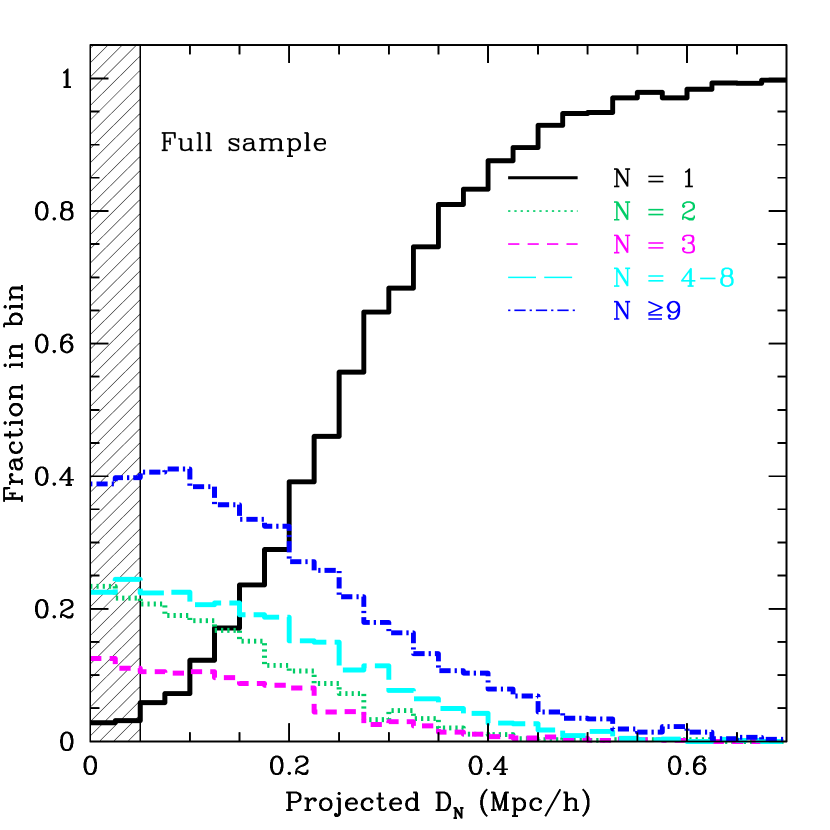
Figure 1.— The fraction of galaxies in the simulation with a total of N galaxies in their host halos as a function of ${\rm D_{N}}$, the projected distance to its nearest neighbor. For each galaxy in the mock catalog, we measure ${\rm D_{N}}$ within $\Delta V$$=1000$ km s^-1, and the total number of galaxies in its host halo, N. The different lines correspond to different bins of N, N $=1$ exactly (solid black), 2 (dotted green), 3 (dashed magenta), 4-8 (long-dashed cyan), and $\geq 9$ (dot-dashed blue) galaxies in the host halo. We shade the “pair zone,” galaxies with neighbors within 50 h^-1 kpc. Close pairs are preferentially found in very well-populated halos.

We begin our exploration of close pair selection in Figure 1. To construct this figure, we first compute ${\rm D_{N}}$ and N for each simulated galaxy, using the periodic boundary conditions, if necessary, to fully sample its environment. We then split the objects in each bin of ${\rm D_{N}}$ into subsets based on the multiplicities of the halos in which the objects reside, $N_{gal}(\mathrm{N}|\mathrm{D_{N}})$. The ranges of the N bins are shown in the labels of Fig. 1. Finally, at each value of projected nearest-neighbor separation, we computed the fraction of galaxies within that bin that are in the different subsets of N. Fig. 1 shows this fraction among five different bins of N as a function of ${\rm D_{N}}$. In each ${\rm D_{N}}$ bin, the sum of all fractions is 1. For reference, the shaded region indicates the 50 h^-1 kpc “pair zone.” We note that the x-axis, ${\rm D_{N}}$, is the directly measurable quantity from redshift survey data, while N is not directly measurable.

Fig. 1 immediately reveals a major issue in selecting appropriate control samples for galaxies in pairs. Pairs in the simulation reside in a highly skewed distribution of environments. In particular, pairs are vastly over-weighted toward galaxies that reside within well-populated host dark matter halos compared to the average. For example, galaxies with N $\geq 9$ comprise 39% of the pair sample but only 19% of the simulation as a whole. In contrast, while isolated (N=1) galaxies make up 56% of the simulation as a whole, only 3% of the apparent close pairs are actually isolated galaxies. These isolated galaxies in apparent pairs are interlopers according to the analysis of Berrier et al. (2006). The abundant pairs in cluster and large-group systems are not necessarily imminent mergers, nor are they necessarily even interacting directly with each other. Bailin et al. (2007) note a similar problem in the study of galactic satellite populations.

From a qualitative perspective, Figure 1 explains many past observations regarding the star-forming properties of galaxies in pairs. For example, pair samples previously analyzed in the 2dFGRS show an increased star formation rate relative to control samples at close separations ($\Delta D$$\lesssim 30$ h^-1 kpc) where the interaction has a dominant effect (Lambas et al., 2003). However, at larger separations where the interaction is less important ($100\lesssim{\rm\Delta D}\leq 200$ h^-1 kpc), the typical pairs exhibit less star formation than the field (e.g., Lambas et al., 2003; Alonso et al., 2004, 2006). In our model, these more widely-separated pairs are also in denser environments than the field: 36% are in N $\geq 9$-galaxy halos while only 19% are isolated. This depressed star formation in widely-separated pairs relative to the field results from the fact that galaxies living in more massive and populated systems have suppressed star formation on average.

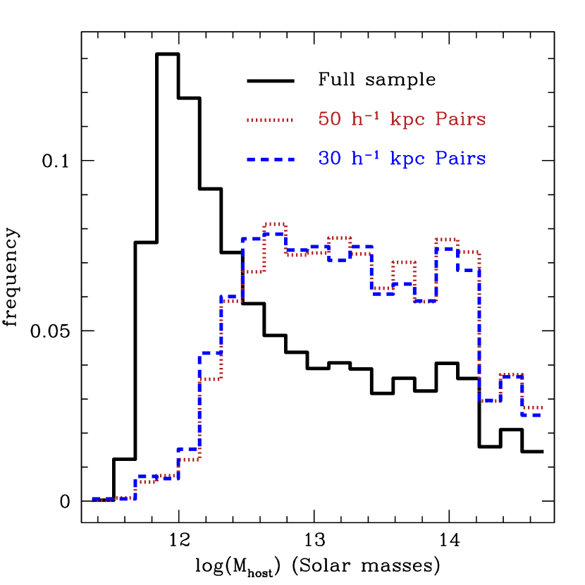
Figure 2.— The normalized distribution, ${\rm d}n/{\rm d}\log(M)$, of host halo masses for 50 h^-1 kpc pairs (dotted red), closer 30 h^-1 kpc pairs (dashed blue) and the full sample (solid black) in the simulation. Pairs reside in much more massive halos than typical “field” galaxies.

Because pairs are preferentially found in denser environments, the naive comparison of star formation rates between pairs and typical field galaxies will artificially underestimate any elevation in star formation rate that is directly triggered by an interaction. Fig. 2 shows the distribution of host halo masses for galaxies in close ($\Delta D$$\leq 50$ and 30 h^-1 kpc) pairs and the sample as a whole. This Figure emphasizes how skewed the environments actually are. The average host halo mass for the full sample is ${\rm<M_{\rm host}>=3.2\times 10^{13}}$ h${}^{-1}\ M_{\sun}$; for the close (50 h^-1 kpc) and closer (30 h^-1 kpc) samples of pairs it is 6.0 and 5.7$\times 10^{13}\ {\rm h^{-1}\ M}_{\sun}$, respectively. Moreover, the mode of the full sample, $\sim 10^{12}\ {\rm h^{-1}\ M}_{\sun}$, is almost completely depleted in the pair sample. The analysis of the SDSS by Weinmann et al. (2006) tracks the dependence of galaxy properties on host halo mass. We can use their results to understand the implications for galaxies in pairs, which are preferentially selected from higher-mass halos. According to their results the “average” color of a galaxy in an “average” halo hosting a pair would be $\sim$0.05 magnitudes redder in ${\rm g-r}$ color, have a specific star formation rate (e.g., Brinchmann et al., 2004) that is $\sim$20% lower, and have a late-type fraction that is $\sim$5% lower than the corresponding averages for the field. Thus, the suppressed star formation observed in some widely-separated galaxy pairs is not related to a single interaction, but is a selection effect associated with cluster and group processes that suppress star formation. This selection effect must be accounted for in a fair analysis of triggered star formation.

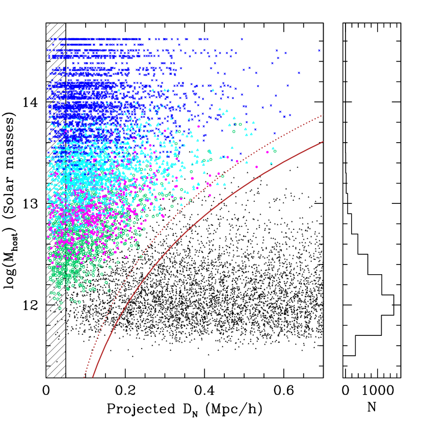
Figure 3.— The distribution of host halo mass as a function of distance to the nearest neighbor, ${\rm D_{N}}$, in the simulation for a single realization of the substructure model. (Left) For galaxies with at least one luminous neighbor within 700 h^-1 kpc and $\Delta V$$=1000$ km s^-1, we plot the log of the host halo mass as a function of projected distance to the nearest neighbor in the simulation. The point colors and types segregate galaxies based on halo occupation. We plot single-galaxy halos (solid black triangles), N $=2$ (open green circles), 3 (filled magenta circles), 4-8 (open cyan triangles), and $\geq 9$-galaxy halos (blue crosses). The solid red line is the virial radius of halos; the dotted red line is the virial radius reduced by a factor of $\sqrt{2/3}$ to account for the typical difference between projected and actual separation. (Right) We also plot the host mass histogram of the host halo of simulated galaxies with no neighbors within 700 h^-1 kpc.

Fig. 3 illustrates the nature of the differences between halos that host close pairs and “typical” dark matter halos. This figure plots galaxy host halo mass as a function of projected separation to its nearest neighbor up to 700 h^-1 kpc and within 1000 km s^-1 in our mock catalogs. The colors and point types segregate host halos based on N, the number of galaxies they host. The structure of this plot provides a very general means of viewing nearest-neighbor statistics. The isolated halos line up along the lower part of the plot; their locus is analogous to the “two-halo” term in the correlation function insofar as the pairs are projections of two coincidentally aligned host halos. The more massive and populated dark matter halos line up along the left vertical edge of the plot. Again, pairs are an extremely skewed population. In contrast, galaxies that are isolated within $\sim$400-500 h^-1 kpc are almost purely the only occupants in their lower-mass halos.

In summary, a comparison of the properties of typical pairs and typical isolated galaxies selected from the universe as a whole is not the appropriate comparison for isolating star formation triggered by galaxy interactions. The “field” is dominated by isolated, low-mass host halos with a mix of a few more luminous systems. Pairs are skewed, preferentially residing in higher-mass host halos. Thus, comparisons of the star-forming properties of pairs and the “field” do not isolate the effects of the recent interaction. The properties of close pairs reflect all of the other processes that occur in dense group and cluster environments that may act to suppress star formation during late-time interactions. As such, naive comparisons will dramatically underestimate the rise in star formation rate triggered by galaxy interactions. In the next section, we describe one means of constructing samples that better isolate the effects of galaxy interactions from other environment-related processes.

4. Isolating triggered star formation

Many different measures of large-scale environment have been developed to understand the properties of galaxies as a function of their surroundings. With the advent of redshift surveys, these studies have focused on group-finding algorithms (Huchra & Geller, 1982), nth nearest neighbor statistics (Dressler, 1980), and local galaxy count measures (e.g., Blanton et al., 2005a; Berrier et al., 2007). Here, we adopt ${\rm N_{700}}$, the number of neighboring galaxies within 700 h^-1 kpc on the sky and $\Delta V$$=1000$ km s^-1 in redshift of the galaxy in question (see Berrier et al., 2007). We note that our results are qualitatively insensitive to choices of environment statistic scale in the range of 700-1000 h^-1 kpc, but 700 h^-1 kpc yields a large enough sample of galaxies in pairs in the 2dFGRS (§ 5). The use of other statistics such as group-finding algorithms would yield somewhat different results, but the basic problem of separating dense systems from nearby but unassociated isolated dark matter halos remains.

Choosing galaxies with limited numbers of companions on $\sim$1 Mpc scale environments is an effective way to preferentially select galaxies in different types of dark matter halos (see Focardi et al., 2006). Fig. 4 shows the distribution of projected ${\rm D_{N}}$ as a function of host halo mass for the the restricted set of environments corresponding to galaxies with ${\rm N_{700}}$ $=1$. These are galaxies that have exactly one companion within 700 h^-1 kpc and 1000 km s^-1. This restriction is extremely clean and effective. Widely-separated pairs are almost exclusively isolated halos and the close pairs are almost purely N $=2$ systems. Fig. 5 shows the fraction of host halos of each type as a function of separation in this restricted sample and the corresponding host halo masses in the pairs and full distributions. The fraction of N $=2$ hosts goes from over 90% at the closest separations to a $50/50$ split of N $=1$ and N $=2$ halos at $\sim$175 h^-1 kpc, to nearly 100% N $=1$ halos beyond 400 h^-1 kpc.

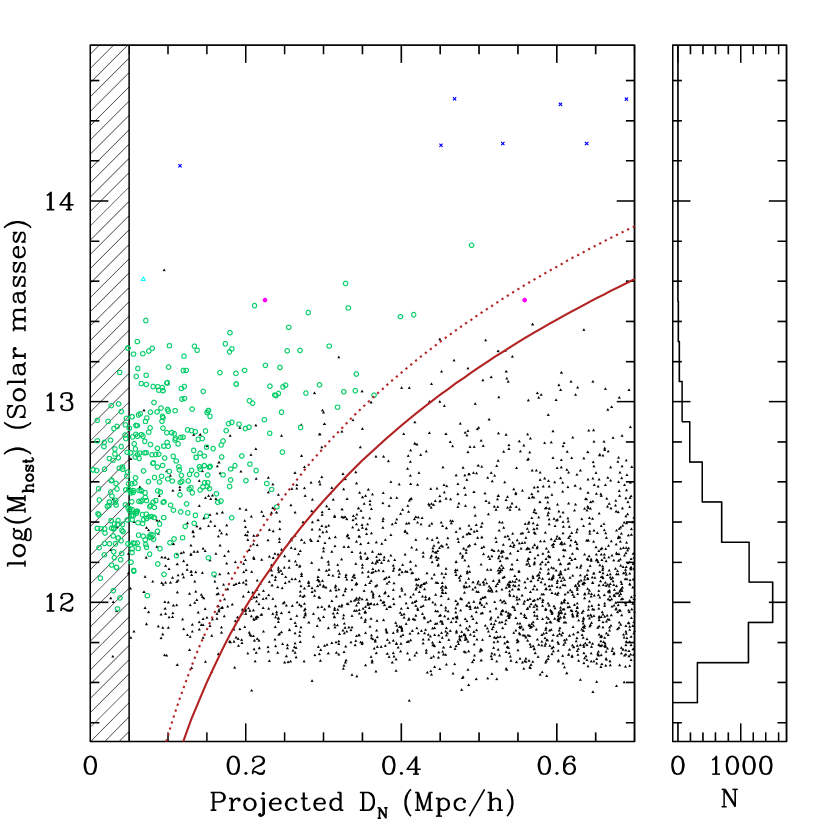
Figure 4.— The distribution of host halo mass as a function of distance to the nearest neighbor, ${\rm D_{N}}$, in the lowest-density environments for the objects in one realization of our mock galaxy catalogs. The points are the same as Fig. 3, but restricted to galaxies with exactly one neighbor within 700 h^-1 kpc and $\Delta V$$=1000$ km s^-1. At right, we plot the host mass histogram of galaxies with ${\rm N_{700}}$ $=0$, or a nearest neighbor distance ${\rm D_{N}}$ $\geq 700$ h^-1 kpc.

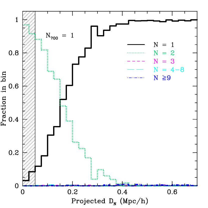
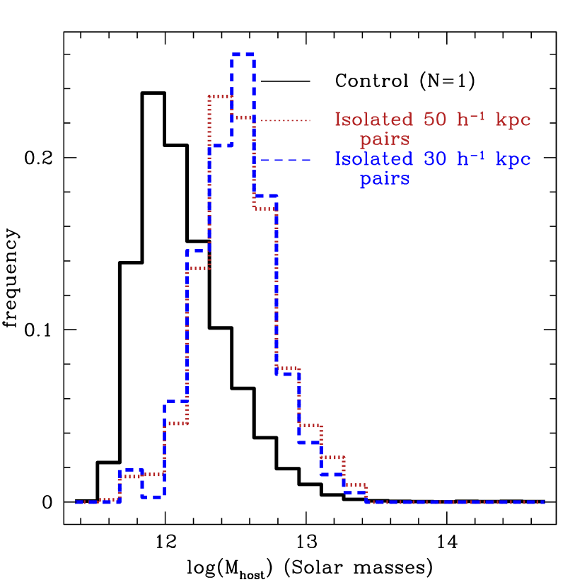
Figure 5.— The distribution of host halo masses and separations in low-density environments in our mock catalogs. We repeat Figs. 1 and 2 restricting to galaxies with ${\rm N_{700}}$ $=1$, or exactly one luminous neighbor within 700 h^-1 kpc. In the left panel, we plot the fraction of galaxies in hosts with a given number of members, N, as a function of the distance to the nearest neighbor within 1000 km s^-1. At right, we plot histograms, ${\rm d}n/{\rm d}\log(M)$, of host halo masses for the control sample of ${\rm N_{700}}$ $\leq 1$ galaxies with ${\rm D_{N}}$ $\geq 300$ h^-1 kpc (black, solid) and for $\leq 50$ h^-1 kpc pairs with no other neighbors within 700 h^-1 kpc (red, dotted) and similarly isolated $\leq 30$ h^-1 kpc pairs (blue dashed). The isolated pairs are twice as massive, on average, as the isolated control sample, implying that the control galaxies are likely the immediate progenitors of the pairs.

The key to the use of ultra-low-density environments is that the restriction provides an extremely clean sample of pairs in N $=2$ halos at small separations and a corresponding control sample of isolated galaxies. This allows us to remove any effects that may be due to numerous and repeated interactions in dense cluster environments and study the relative effect of individual interactions. The sample average masses are ${\rm<M_{\rm host}>=4.2}$ and ${3.9\times 10^{12}}$ h${}^{-1}\ M_{\sun}$, respectively, for the objects that could be identified as isolated 50 h^-1 kpc and 30 h^-1 kpc close pairs, and ${\rm<M_{\rm host}>=2.2\times 10^{12}}$ h${}^{-1}\ M_{\sun}$ for the simulated isolated galaxy sample with ${\rm D_{N}}$ $>300$ h^-1 kpc and ${\rm N_{700}}$ $=0$ or 1. The peaks in the distributions are offset by $\sim$0.5 dex. Thus, isolated close pair host halos are $\sim$2 – 3 times the typical masses of the isolated galaxy (N $=1$) sample, suggesting that the isolated galaxies are the appropriate immediate progenitors of the N $=2$ isolated close pairs. In the simulation, the subhalos we would identify observationally as isolated close pairs were accreted roughly 0-8 Gyr ago, with an average of 3.0 Gyr and a wide spread of $\sigma=1.5$ Gyr. For comparison, the dynamical timescales for these halos are of order $3$ Gyr.

As a guide to interpreting this isolated sample, consider a simple example. At present, the Milky Way and the Andromeda galaxy, viewed from most projections, would be black points on the right side of Fig. 4. They are both isolated with respect to luminous galaxies. However, as they move toward one another over the course of the next $\sim$few Gyr (Cox & Loeb, 2007), they will move to the left on the plot. Eventually their dark matter halos merge and they become an N $=2$ halo, at which time they will move diagonally toward the upper left and “turn green.” After perhaps 1-3 Gyr, the baryonic galaxies will completely coalesce; the system would then move horizontally to the right and “turn black” in the plot. Isolated systems like the Milky Way and Andromeda are the simplest units of interaction and the best laboratories to isolate the effects of interactions from other physical processes. In the next section, we find isolated pairs in the 2dFGRS and use the appropriate control and paired samples to isolate the effects of an interaction. As we show in § 7, the situation is much more complex in denser environments.

5. Measuring triggered star formation

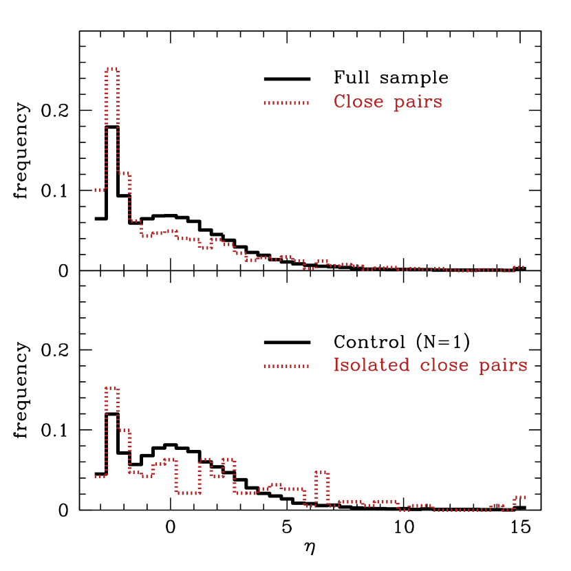
[b]

Figure 6.— Star-forming properties of 2dFGRS galaxies in pairs. (Top) We plot the distribution of $\eta$ for the volume-limited sample as a whole (solid, black) and for the close pairs sample (dotted, red) with ${\rm D_{N}}$ $\leq 50$ h^-1 kpc. Larger values of $\eta$ correspond to higher star formation rates (Madgwick et al., 2003). Relative to the sample as a whole, the pairs exhibit less star formation on average, as explained in Fig. 1 by the fact that they preferentially sample dense galactic environments. (Bottom) We also restrict to isolated close pairs (dotted, red) and a control sample of galaxies with a ${\rm N_{700}}$ $\leq 1$ and ${\rm D_{N}}$ $\geq 300$ h^-1 kpc distant on the sky. The model shows that the pairs are almost always in N $=2$ halos (93%) and that 99.5% of the control sample are in N $=1$ halos. Relative to the isolated “control” galaxies, the isolated pairs have more galaxies on both ends of the $\eta$ distribution.

In § 4, we demonstrate that the amount of triggered star formation occurring in the universe cannot be measured by comparing typical paired galaxies to typical field galaxies. Dense galactic environments are overrepresented in galaxies in pairs. However, the effects of an interaction can be identified independent from other environmental processes by examining isolated pairs and comparing them to isolated galaxies. Although isolated pairs are not the only environments in which triggered star formation is important, they are the simplest to identify and study.

Here, we use 2dF survey pairs to examine triggered star formation in galaxy pairs. The “full sample” is the full volume-limited sample that is far enough away from the edge of the survey to sample the environments of galaxies without bias. The “close pairs” sample is the subset of this full sample that has at least one companion within 50 h^-1 kpc and 1000 km s^-1. We focus on the clean measure of the effects of interactions described in § 4 by constructing the “isolated close pairs” sample of galaxies that have exactly one companion within 50 h^-1 kpc and 1000 km s^-1 and no others within 700 h^-1 kpc and 1000 km s^-1. We also construct the “control” sample where ${\rm N_{700}}$ $=0$ or 1 and the nearest neighbor is ${\rm D_{N}}$ $\geq 300$ h^-1 kpc away.

In the volume-limited sample of 41,239 galaxies, the “full sample” includes 22,601 galaxies that are not on the edges of the survey volume. There are 1344 galaxies in the “close pairs” sample, with spectroscopic companions within 50 h^-1 kpc and 1000 km s^-1; 191 of these paired galaxies are in isolated close ($\leq 50$ h^-1 kpc) pairs and 72 are in isolated closer ($\leq 30$ h^-1 kpc) pairs. The isolated control sample with ${\rm D_{N}}$ $\geq 300$ h^-1 kpc and ${\rm N_{700}}$ $=0$ or 1 includes 8564 galaxies.

We examine the star-forming properties of galaxies using the spectral parameter $\eta$, which Madgwick et al. (2002) derive from principal component analysis (PCA) of the 2dFGRS as a whole. Their PCA analysis shows that two-thirds of the variance in the 2dFGRS spectra in a volume-limited sample are contained in the first two projections. $\eta$ is directly measured from a combination of these two projections and is readily available in the 2dFGRS database. Madgwick et al. (2003) show that $\eta$ is closely related to both the H$\alpha$ equivalent width measured from spectra and to the stellar birthrate parameter, $b$, the present star formation rate of the galaxy divided by its average past star formation rate. Higher values of $\eta$ correspond directly to higher current star formation rates. Madgwick et al. (2003) use model spectral energy distributions with a wide variety of star formation histories to explore this correlation between $\eta$ and $b$.

In the top of Fig. 6 we plot the distribution of $\eta$ for the sample as a whole and all the close pairs. The pairs as a whole exhibit, on average, less overall star formation than the full volume-limited galaxy sample. The average for the full sample and the close pairs sample are $<\eta>=0.07$ and -0.22, respectively. Fig. 1 demonstrates why. In the model, most (56%) galaxies are alone in their dark matter halos. In $\leq 50$ h^-1 kpc pairs, however, nearly all (97%) of the galaxies are in denser systems, and often much denser systems. Because pairs preferentially reside in extremely dense environments, their star formation is suppressed except when they are strongly interacting.

As we demonstrate in § 4, the model predicts that 99.5% of the galaxies in the isolated control sample are alone in their dark matter halos and that 93% of the isolated pairs are in N $=2$ halos. Thus, the bottom of Fig. 6 provides us with a nearly direct measure of the effects of an interaction, by allowing us to compare the true progenitors (the N $=1$ “control”) of the paired (N $=2$) systems. A Kolmogorov-Smirnov test indicates that the control and close-pair $\eta$ distributions differ, with P${}_{\rm K-S}=6.1\times 10^{-4}$.

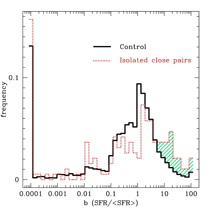
[b]

Figure 7.— Normalized star formation rates of 2dFGRS galaxies in pairs. We plot the distribution of $b$, the ratio of the current star formation rate to the average past star formation rate, inferred from $\eta$ (see Madgwick et al., 2003). We restrict to isolated close pairs (dotted, red) and a control sample of galaxies with ${\rm N_{700}}$ $\leq 1$ and ${\rm D_{N}}$ $\geq 300$ h^-1 kpc. A Kolmogorov-Smirnov test indicates that the control and close-pair $\eta$ distributions differ, with P${}_{\rm K-S}=6.1\times 10^{-4}$. Relative to the N $=1$ “control” galaxies, the isolated pairs have fewer galaxies forming stars at their historical average rate; pairs exhibit an excess of galaxies that are very deficient in star formation (5% excess with $b\leq 0.1$) and an excess of galaxies (green shaded region) with rates boosted by factors of $\gtrsim 5$ (14%) where the high-$b$ excess, or the shaded region, has an average $\left<b\right>\sim 30$.

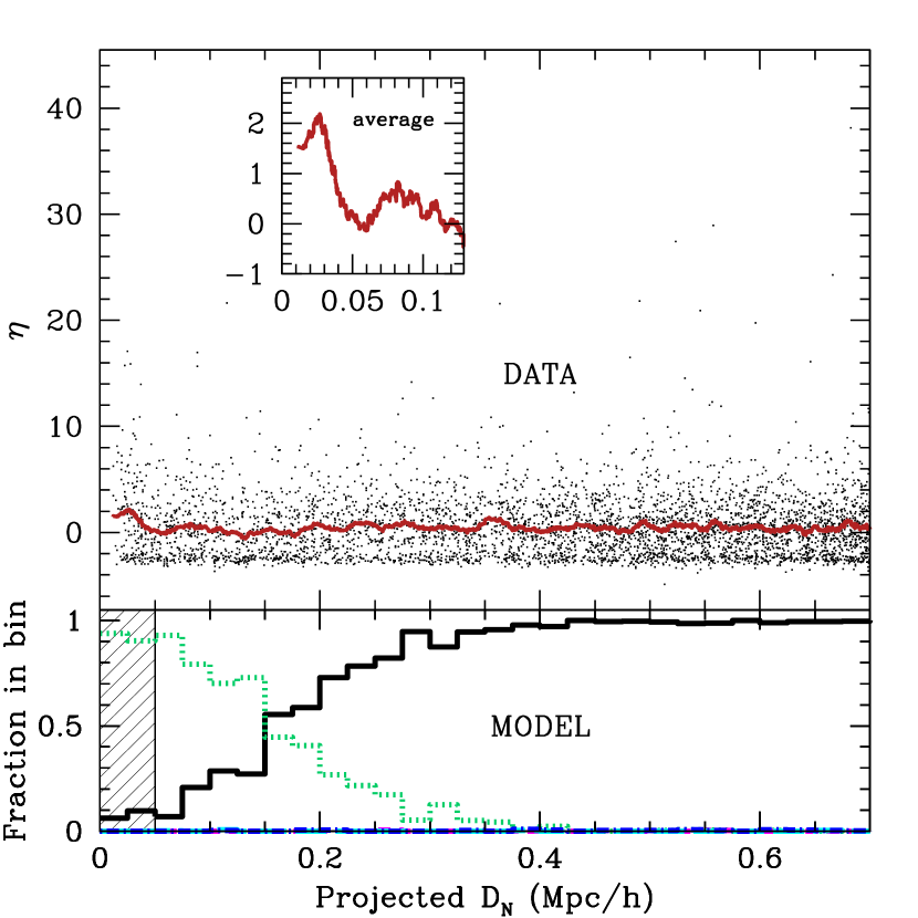
[b]

Figure 8.— Star formation as a function of distance to nearest neighbor in sparse environments. (Top) For the 2dFGRS sample with ${\rm N_{700}}$ $=1$, we plot $\eta$ as a function of separation to the nearest neighbor; the red line is the averaged smoothed by 100 points. The inset displays the average for ${\rm D_{N}}$ $\lesssim 0.13$ h^-1 Mpc, highlighting the signal of triggered star formation at ${\rm D_{N}}$ $\lesssim 0.03$ h^-1 Mpc. (Bottom) For the ${\rm N_{700}}$ $=1$ sample in the simulation, we plot the fraction of N $=1$ (solid, black) and N $=2$ (dotted, green) galaxies as a function of ${\rm D_{N}}$, as in Fig. 5.

In Fig. 7, we use the approximate values in Figure 7 of Madgwick et al. (2003) to convert $\eta$ into $b$, the ratio of the current star formation rate to the average past star formation rate, for the isolated control and isolated pairs samples only. Relative to the N $=1$ “control” galaxies, the isolated pairs have fewer galaxies forming stars at their historical average rate ($b\sim 1$). Pairs include an excess of low- and high-star-formation-rate galaxies. While 24% of the control sample are forming stars with $b<0.1$, 29% of the $<50$ h^-1 kpc pairs and 26% of the $<30$ h^-1 kpc are forming stars at these low rates; thus, 50 h^-1 kpc (30 h^-1 kpc) pairs have a 5% (2%) excess of slow (or non-) star formers.

At the high end of the star-formation rate distribution, 10% of the control (N $=1$) sample have rates boosted by $\gtrsim$ a factor of 5. In contrast, 50 h^-1 kpc (30 h^-1 kpc) pairs are boosted by $b\geq 5$ 24% (30.5%) of the time, for a 14% (20%) excess of high star formation rate galaxies. Binning the data with fine bins, weighting by $b$, and limiting the largest (extrapolated) boost to $b=100$, the high-$b$ ($b>5$) excess in the pairs, the shaded region in Fig. 7, has an average of $b\sim 31$ (34). In other words, statistically, this technique shows that for the population of pairs with triggered star formation, the average boost in the star formation rate over the average past rate in that galaxy is a factor of $\sim$30.

The error in the average boost due to triggered star formation is dominated by the scatter in the relationship between the physical parameter $b={\rm SFR/\left<SFR\right>}$ and the measured $\eta$. We estimate the error introduced by this scatter using a Monte-Carlo simulation. Madgwick et al. (2003) explore the scatter in the theoretical relationship between $b$ and $\eta$ using synthetic spectra with star formation histories predicted by semi-analytic models. For a typical distribution of star formation histories, this scatter is substantial. We adopt the 1-$\sigma$ scatter in the $\eta$-$b$ distribution in Madgwick et al. (2003) in our Monte Carlo simulation, drawing deviations at random from the average $b$ for a given (measured) $\eta$. We resample the entire $b$ distribution for the control, pair, and very close (30 h^-1 kpc) pair $\eta$ distributions and remeasure the weighted average boost of the excess strong star formers with $b>5$ in the pairs. Because the scatter of $b$ as a function of $\eta$ is much larger in the high-$b$ direction, the 1-$\sigma$ range of resulting values of the average boost of triggered star formation is 42 – 65 for the 50 h^-1 kpc pairs and 39 – 61 30 h^-1 kpc pairs. We conclude from this analysis that the large scatter between $b$ and $\eta$ results in a wide range of possible star formation boosts resulting from triggered star formation. This type of uncertainty would be typical for other popular parameterizations of star formation history derived from optical spectra, as well. Many optical spectral measures of star formation break down in the “bursty” star formation regime that is typical of interacting galaxies.

The excess fraction of starbursting galaxies is enhanced in even closer (30 h^-1 kpc) pairs, while the excess of low star formation rate galaxies is not. We explore the dependence of starbursting galaxies on separation further by dividing the data into bins based on ${\rm D_{N}}$. With 50 h^-1 kpc bins, only the ${\rm D_{N}}$ $\leq 50$ h^-1 kpc bin has a statistically significant excess of high-$b$ galaxies compared with the N $=1$ control; with 25 h^-1 kpc bins, only the ${\rm D_{N}}$ $\leq 50$ h^-1 bins show a significant excess.

6. Understanding the trends

These trends with separation on the sky have been noted previously by several authors using many different pair datasets (Barton et al., 2000; Lambas et al., 2003; Nikolic et al., 2004; Alonso et al., 2004, 2006; Lin et al., 2007). Thus, the fact that we reproduce them here is not surprising. However, as Figs. 1 and 5 show, all pair samples suffer from systematic environmental differences as a function of separation on the sky that are not directly related to interactions. Typical galaxy samples with no environmental controls are dominated by cluster galaxies at separations $\lesssim 200$ h^-1 kpc and field galaxies at separations $\gtrsim 200$ h^-1 kpc. Even the most isolated samples of pairs are dominated by pairs in N $=2$ halos at separations $\lesssim 200$ h^-1 kpc and by N $=1$ halos at separations $\gtrsim 200$ h^-1 kpc. Here, for the first time, we are uniquely poised to explore these effects and construct appropriate control samples using models.

Although we note that isolated galaxies in pairs are the simplest interactions to study and compare with isolated galaxies, they still may be affected by other processes. N $=2$ halos are often the result of the merger of two N $=1$ systems, but they can also result from an N $=3$ system after two of the three baryonic galaxies coalesce. An origin as a N $=3$ system is, however, much less likely for a given system. Although our models are not presently capable of tracking these mergers in detail, we note that the density of N $=3$ is only 8% of the density of N $=1$ systems. Thus, the simplest interpretation of the result in Fig. 7 is that the 5% excess of low-star-formation systems in the N $=2$ galaxies results from the fact that galaxies in N $=2$ halos are more likely than isolated galaxies to have experienced previous gas-consuming interactions, and that the 14% excess of strongly star-forming galaxies in N $=2$ halos results directly from recent interactions. Future investigation of these models will clarify this evolution.

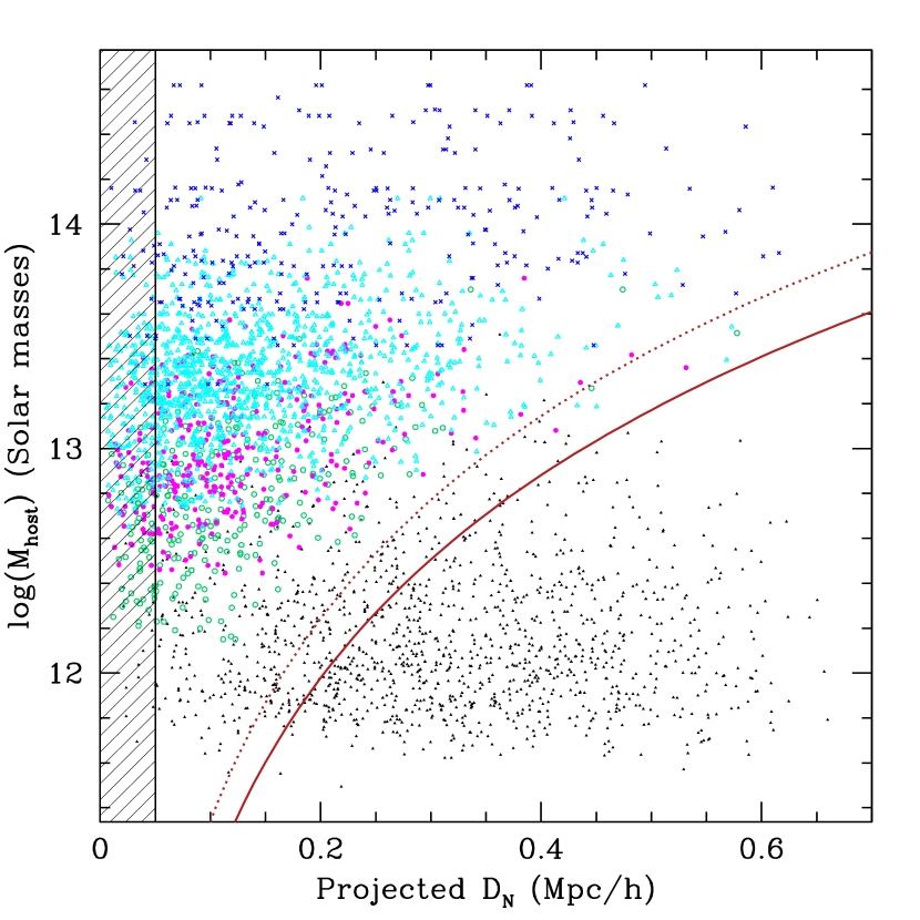
Figure 9.— Denser environments: the distribution of host halo mass as a function of distance to the nearest neighbor, ${\rm D_{N}}$, but restricted to galaxies with 3-8 neighbors within 700 h^-1 kpc and $\Delta V$$=1000$ km s^-1. The points are the same as Fig. 3.

Supporting this picture, the boosted star formation does not extend to all systems with N $=2$. In Fig. 8, we plot $\eta$ as a function of separation for the isolated (${\rm N_{700}}$ $=1$) sample. A high mean $\eta$ persists only out to $\sim$40-50 h^-1 kpc. However, the model plotted below the points for clarity shows that the N $=2$ halos dominate well past 100 h^-1 kpc. Thus, the boosted star formation at small separations results from the physical interaction and not merely the different mix of halo types at smaller separations. A boosted average star formation rate does not persist beyond a few tens of h^-1 kpc, probably because the strength of the star formation fades as the burst ages (see Barton et al., 2000; Barton Gillespie et al., 2003), and because the fraction of galaxies that have had a recent close pass is a strong function of ${\rm D_{N}}$.

The halo substructure model tracks close pericentric passages between satellites and the central galaxy in the dark matter host halo. These simulations show that for the isolated close pair galaxies in true N $=2$ systems, 12% of the $\leq$50 h^-1 kpc pairs and 16% of the $\leq$30 h^-1 kpc pairs have had a close pass with R${}_{\rm peri}<30$ h^-1 kpc within the last Gyr. In addition, 40% of the 50 h^-1 kpc pairs and 45% of the 30 h^-1 kpc pairs have had a pass with R${}_{\rm peri}<50$ h^-1 kpc within the last 1.2 Gyr. Thus, the 2dF data are consistent with a range of scenarios, including at its extremes, (1) the possibility that nearly all galaxies with $<30$ h^-1 kpc passes burst by an average factor of $\sim$30 for 1 Gyr, or (2) the possibility that $\lesssim$ half of the galaxies with $<50$ h^-1 kpc passes burst this much for $\sim$1.2 Gyr. If star formation continues for these long timescales, more widely-separated pairs will contain some systems with triggered star formation. However, the average star formation rate at wider separations is not affected because pairs that have had close passes are diluted. The model shows that only 3% of the true N $=2$ systems with separations $100<$ ${\rm D_{N}}$ $<200$ h ^-1 kpc have had a close ($<30$ h^-1kpc) pass within the last Gyr.

We will attempt further exploration of these scenarios in later work. However, preliminary analysis of Sloan Digital Sky Survey DR4 NYU Value-Added Galaxy Catalog data York et al. (2000); Blanton et al. (2005b); Adelman-McCarthy et al. (2006) — albeit with quite different star formation measures — suggests that the bursting fraction is a strong function of the cutoff luminosity of the sample studied. The fraction also depends in detail on the star formation measure and on the luminosity cutoff used for constructing the volume-limited sample, probably because star formation rate is a strong function of galaxy luminosity. Qualitatively, the results remain quite consistent between the 2dF and SDSS samples.

The optical spectra available in the 2dFGRS (and the SDSS) do not measure the amount of star formation that is embedded in dust clouds. Thus, the typical boost of the high-$b$ excess provides an approximate lower limit to the amount of triggered star formation in a close galaxy-galaxy pass. As Cox et al. (2006) demonstrate, high-resolution hydrodynamical simulations predict a wide range of star formation boosts from these close passes. Their models predict SFR boosts of 6 – 20 above a galaxy’s isolated star formation rate in prograde encounters during the $\sim$ Gyr between the first close pass and the final merger. Surprisingly, our estimate of $<b>\sim 30$ averaged over the galaxies that have triggered star formation exceeds this range. However, the uncertainties associated with the mapping between $\eta$ and $b$ are substantial. Thus, this 2dF analysis remains broadly consistent with the models described in Cox et al. (2006) and does not yet distinguish among them.

6.1. The effects of survey incompleteness

The 2dFGRS is not spectroscopically complete; the survey is especially deficient in close pairs. We examine the effects of incompleteness using the measured completeness of the sectors in which the galaxies fall, and the 2dF parameters “wsel,” a weighted measure of whether the ten nearest galaxies have high-quality redshifts, and “bjlim,” the limiting magnitude of the relevant sector (Colless et al., 2001; Norberg et al., 2002). Restricting the sample to sectors with known completeness $>90\%$ and with wsel $\geq 1.3$ and bjlim $\geq$19.35, we find a reduced isolated pairs sample with only 67 pair galaxies and 2132 control galaxies. As a result, a K-S test no longer reveals any statistical significance of the difference in $\eta$ distributions (P${}_{\rm K-S}=0.35$). Nevertheless, the differences in star-forming properties of the isolated control and isolated remain qualitatively unchanged: in the restricted control sample, 12% of the galaxies have $b>5$; in the restricted isolated pairs, 21% have $b>5$. Thus, contamination of the isolated control sample appears to have no significant effects on our results.

We further test the effects of redshift survey completeness by applying the same analysis to the SDSS DR4 sample (Blanton et al., 2005b; Adelman-McCarthy et al., 2006). Although the detailed results are beyond the scope of this paper, we are able to use SDSS to find a pure isolated pair sample and a pure control sample with SDSS. We construct these samples because we are able to exclude all systems with neighbors that have unmeasured redshifts. The measured excess of star formation in isolated pairs compared with the control sample, from SDSS depends sensitively on the cutoff luminosity of the volume-limited sample. This dependence arises because higher-luminosity galaxies have less star formation in general. Using H$\alpha$ equivalent width as a measure of star formation, the measured excess of pairs with EW(H$\alpha$) $\geq 25$ Å ranges from somewhat lower than the 2dF results we present here (4%) for a sample volume limited to M${}_{r}=-20+5\log{h}$ to 19% for a sample volume limited to M${}_{r}=-19+5\log{h}$. The 2dF luminosity limit corresponds to galaxies that are midway between these numbers. Thus, the 2dF and SDSS analyses agree qualitatively, and the fraction of galaxies in close pairs with triggered star formation increases when lower luminosity galaxies are included. The differences may result from the use of very different measures of star formation or from the use of galaxies in an intrinsically different luminosity range. However, this analysis suggests that “impurity” in the 2dF sample — the inclusion of galaxies and pairs that are not truly isolated — is not biasing our results significantly.

7. More complex environments

Isolated pairs of galaxies are the easiest systems to construct an appropriate control sample for. However, isolated pairs are by no means the only pairs that show evidence for triggered star formation. Alonso et al. (2006) show that $b$ still increases as pair separation on the sky decreases for close pairs in denser environments.

In Sec. 4, we describe the effectiveness of isolating the lowest-density environments to create an appropriate control sample for galaxies in isolated pairs. Unfortunately, the same type of technique does not work for higher-density environments. One cannot separate galaxies into a density bin and expect the non-pairs to be a good control sample for the pairs.

To illustrate this point, we restrict the sample to intermediate values of our environment statistic; in Fig. 9 we plot galaxies with $3\leq$ ${\rm N_{700}}$ $\leq 8$. As expected, isolated N $=1$ halos are missing from the 50 h^-1 kpc pairs sample (3.1%) but still constitute a significant fraction of the overall sample (31%). This result immediately illustrates the problem with breaking sets of galaxies into low, intermediate, and high-density samples and separating the pairs from these samples (e.g., Alonso et al., 2006). The close pairs have a completely different environmental mix from the rest of this intermediate-density sample. The mix is a strong function of distance to the nearest neighbor, and even the pairs reside in a huge range of hosts, from halos with N $=2$ galaxies to halos with N $>9$. However, as Alonso et al. (2006) show, pairs in dense environments do exhibit a rise in star formation rate with a very close encounter.

The ineffectiveness of comparing pairs and “control” galaxies in intermediate- or high-density environments is not merely a result of the exact technique we use. Group-finding algorithms can be tuned to lower the incompleteness and/or impurity rates on various scales (e.g., Yang et al., 2005; Gerke et al., 2005; Weinmann et al., 2006; Berlind et al., 2006; Koester et al., 2007), but these algorithms will always include isolated galaxies in denser systems from the control sample at a higher rate than they appear in the pairs. Because the distribution of star formation rates in isolated galaxies has a high-star-formation tail, their contamination will always lower the measured difference in star formation rate between paired and non-paired galaxies in loose groups. One effective approach in these environments is to estimate the contamination of N $=1$ galaxies to the sample of interest and to statistically subtract its contribution.

What is the appropriate control sample for pairs in dense environments? Even if one could identify the host halo mass and occupation of galaxies perfectly, this would still be a difficult question to answer. The immediate progenitors of pairs in dense environments can range from isolated galaxies that have just fallen into the system to galaxies that have been in a loose group for along time but are just encountering one another for the first time. Tracking the evolution of the orbits of subhalos in the models will reveal the progenitors of interactions in crowded environments, but that analysis is beyond the scope of the present paper.

8. Conclusion

Here, we use mock catalogs based on simulations of cosmological structure formation in the prevailing $\Lambda$CDM model to understand the properties of galaxies in pairs. We examine the typical host dark matter halos of galaxies in apparent pairs in the simulations and find that:

1. Our simulations show that galaxies in close pairs are preferentially located in cluster and group environments. As a result, typical close pairs are not ideal for understanding triggered star formation in galaxy-galaxy interactions. This result explains why galaxies in pairs can appear redder or can appear to have less star formation than the typical “field” galaxies. If the goal is to isolate the effects of a recent interaction, the “field” is not an appropriate control sample with which to compare typical galaxies in close pairs.

2. Using the simulations, we show that close pairs in the sparsest environments, with only one neighbor within 700 h^-1 kpc, provide the simplest situation for isolating the effects of an interaction. Close ($<50$ or $<30$ h^-1 kpc) isolated pairs are almost exclusively in N $=2$ halos (93%). Very isolated galaxies with at most one neighbor within 700 h^-1 kpc that is at least ${\rm D_{N}}$ $\geq 300$ h^-1 kpc away are almost exclusively in N $=1$ halos (99.5%). Thus, isolated field galaxies are the ideal control sample of the progenitors of isolated pairs.

3. We study isolated pairs and galaxies in a volume-limited sample of M${}_{\rm B,j}\leq-19$ galaxies from the 2dFGRS. Isolated pairs with $\Delta D$ $\leq 50$ h^-1 kpc ($\leq 30$ h^-1 kpc) show an excess of both strongly star-forming galaxies and of non-star-forming galaxies when compared to N $=1$ control sample. While 24% of the control sample is forming stars at $b\lesssim 0.1$ of its average past rate, 29% (26%) of the close pairs lack star formation to this extent. In addition, 24% (30.5%) of the pairs are forming stars at $b\gtrsim 5$ times their average past rate while only 10% of the control sample has rates this high. The rapidly-star-forming excess population in the pairs is almost certainly due to the direct effects of the interaction. However, we note that the fraction of galaxies undergoing triggered starbursts is a function of the limiting absolute magnitude of the sample because a much smaller fraction of more luminous galaxies are able to form stars at all.

4. For the isolated close galaxy pairs in the 2dFGRS, the galaxies with triggered star formation have an average star formation boost of $b=$ SFR/$\left<{\rm SFR}\right>\sim 30$.

5. The measurement of the optical boost of $b\sim 30$ for interactions in 2dFGRS is approximate, due in large part to the large scatter in relationship between star formation history and measured optical spectral parameters. The measure also excludes embedded star formation that is not detectable at optical wavelengths. Thus, it is an estimate of the lower limit to the boost in star formation rate caused by triggered star formation. This boost is higher than predictions derived for boosts from triggered star formation using hydrodynamic simulations (e.g., Cox et al., 2006), although the uncertainties are too large to rule out specific models at this stage.

6. By tracking orbits in the substructure model, we show that for the isolated close pair galaxies in true N $=2$ systems, only 12% (16 %) of the 50 (30) h^-1 kpc pairs have had a close pass with R${}_{\rm peri}<30$ h^-1 kpc within the last Gyr, and 40% (45%) have had a pass with R${}_{\rm peri}<50$ h^-1 kpc within the last 1.2 Gyr. Thus, the detection of triggered star formation in 14% (20%) of these L^⋆ and sub-L^⋆ systems in the 2dF data suggest that a large fraction of the galaxies that experience close passes respond with triggered star formation.

References

- Adelman-McCarthy et al. (2006) Adelman-McCarthy, J., Agueros, M. A., Allam, S.S., et al. 2006, ApJS, 162, 38
- Allgood et al. (2006) Allgood, B., Flores, R. A., Primack, J. R., Kravtsov, A. V., Wechsler, R. H., Faltenbacher, A., & Bullock, J. S. 2006, MNRAS, 367, 1781
- Alonso et al. (2007) Alonso, M. S., Lambas, D. G., Tissera, P., & Coldwell, G. 2007, MNRAS, 375, 1017
- Alonso et al. (2006) Alonso, M. S., Lambas, D. G., Tissera, P., & Coldwell, G. 2006, MNRAS, 367 1029
- Alonso et al. (2004) Alonso, M. S., Tissera, P. B., Coldwell, G., & Lambas D. G. 2004, MNRAS, 352, 1081
- Bailin et al. (2007) Bailin, J., Power, C., Norberg, P., Zaritsky, D., & Gibson, B. K. 2007, ArXiv e-prints, 706, arXiv:0706.1350
- Barnes & Hernquist (1992) Barnes, J. E., & Hernquist, L. 1992, ARA&A, 30, 705
- Barton et al. (2001) Barton, E. J., Geller, M. J., Bromley, B. C., van Zee, L., & Kenyon, S. J. 2001, AJ, 121, 625
- Barton et al. (2000) Barton, E. J., Geller, M. J., & Kenyon, S. J. 2000, ApJ, 530, 660
- Barton Gillespie et al. (2003) Barton Gillespie, E., Geller, M. J., & Kenyon, S. J. 2003, ApJ, 582, 668
- Berlind et al. (2006) Berlind, A. A., et al. 2006, ApJS, 167, 1
- Berrier et al. (2006) Berrier, J. C., Bullock, J. S., Barton, E. J., Guenther, H. D., Zentner, A. R., & Wechsler, R. H. 2006, ApJ, 652, 56
- Berrier et al. (2007) Berrier, H. G., et al. 2007, in preparation
- Blanton et al. (2005a) Blanton, M. R., Eisenstein, D., Hogg, D. W., Schlegel, D. J., & Brinkmann, J. 2005, ApJ, 629, 143
- Blanton et al. (2005b) Blanton, M. R., et al. 2005, AJ, 129, 2562
- Brinchmann et al. (2004) Brinchmann, J., Charlot, S., White, S. D. M., Tremonti, C., Kauffmann, G., Heckman, T., & Brinkmann, J. 2004, MNRAS, 351, 1151
- Bryan & Norman (1998) Bryan, G. L. & Norman, M. L. 1998, ApJ, 495, 80
- Chandrasekhar (1943) Chandrasekhar, S. 1943, ApJ, 97, 255
- Chapman et al. (2005) Chapman, S. C., Blain, A. W., Smail, I., & Ivison, R. J. 2005, ApJ, 622, 772
- Colless et al. (2001) Colless, M., et al. 2001, MNRAS, 328, 1039
- Combes (2001) Combes, F. 2001, in “Advanced Lectures on the Starburst-AGN Connection”, Proceedings of a conference held in Tonantzintla, Puebla, Mexico, 26-30 June, 2000. Eds. by I. Aretxaga, D. Kunth, & R. Mújica. Singapore: World Scientific, 2001., p.223
- Conroy et al. (2006) Conroy, C., Wechsler, R. H., & Kravtsov, A. V. 2006, ApJ, 647, 201
- Croton et al. (2005) Croton, D. J., et al. 2005, MNRAS, 356, 1155
- Cox & Loeb (2007) Cox, T. J., & Loeb, A. 2007, MNRAS, submitted arXiv:0705.1170v1 [astro-ph]
- Cox et al. (2006) Cox, T. J., Jonsson, P., Primack, J. R., & Somerville, R. S. 2006, MNRAS, submitted (astro-ph/0503201)
- Cross et al. (2004) Cross, N. J. G., et al. 2004, MNRAS, 349, 576
- Dressler (1980) Dressler, A. 1980, ApJ, 236, 351
- Freedman Woods, Geller, & Barton (2006) Freedman Woods, D., Geller, M. J., & Barton, E. J. 2006, AJ, 132, 197
- Freedman Woods & Geller (2007) Freedman Woods, D., & Geller, M. J.2007, AJ, submitted
- Focardi et al. (2006) Focardi, P., Zitelli, V., Marinoni, S., & Kelm, B. 2006, A&A, 456, 467
- Gerke et al. (2005) Gerke, B. F., et al. 2005, ApJ, 625, 6
- Gunn & Gott (1972) Gunn, J. E., & Gott, J. R., III 1972, ApJ, 176, 10
- Hashimoto, Funato, & Makino (2003) Hashimoto, Y., Funato, Y., & Makino, J. 2003, ApJ, 582, 196
- Huchra & Geller (1982) Huchra, J. P., Geller, M. J., 1982, ApJ, 257, 423
- Joseph et al. (1984) Joseph, R. D., Meikle, W. P. S., Robertson, N. A., & Wright, G. S. 1984, MNRAS, 209,111
- Kannappan, Jansen, & Barton (2004) Kannappan, S. J., Jansen, R. A., & Barton, E. J. 2004, AJ, 127, 1371
- Kennicutt & Keel (1984) Kennicutt, R. C., Jr., & Keel, W. C. 1984, ApJ, 279, 5
- Kennicutt et al. (1987) Kennicutt, R. C., Jr., Roettiger, K. A., Keel, W. C., van der Hulst, J. M., & Hummel, E. 1987, AJ, 93, 1011
- Kewley et al. (2006) Kewley, L. J., Geller, M. J., & Barton, E. J. 2006, AJ, 131, 2004
- Klypin et al. (1999) Klypin, A., Gottlöber, S., Kravtsov, A. V., & Khokhlov, A. M. 1999, ApJ, 516, 530
- Koester et al. (2007) Koester, B. P., et al. 2007, ApJ, 660, 221
- Kolatt et al. (1999) Kolatt, T. S., et al. 1999, ApJ, 523, L109
- Kormendy & Kennicutt (2004) Kormendy, J., & Kennicutt, R. C., Jr. 2004, ARA&A, 42, 603
- Kravtsov et al. (2004) Kravtsov, A. V., Berlind, A. A., Wechsler, R. H., Klypin, A. A., Gottlöber, S., Allgood, B., & Primack, J. R. 2004a, ApJ, 609, 35
- Kravtsov et al. (1997) Kravtsov, A. V., Klypin, A. A., & Khokhlov, A. M. 1997, ApJS, 111, 73
- Lambas et al. (2003) Lambas, D. G., Tissera, P. B., Alonso, M. S., & Coldwell, G. 2003, MNRAS, 346, 1189
- Larson & Tinsley (1978) Larson, R. B, & Tinsley, B. M. 1978, ApJ, 219, 46
- Lin et al. (2004) Lin, L., et al. 2004, ApJ, 617, L9
- Lin et al. (2007) Lin, L., et al. 2007, ApJ, 660, L51
- Lowenthal et al. (1997) Lowenthal, J. D., et al. 1997, ApJ, 481, 673
- Luo et al. (2007) Luo, Z.-J., Shu, C.-G., & Huang, J.-S. 2007, PASJ, in press
- Madgwick et al. (2002) Madgwick, D. S., et al. 2002, MNRAS, 333, 133
- Madgwick et al. (2003) Madgwick, D. S., Somerville, R., Lahav, O., & Ellis, R. 2003, MNRAS, 343, 871
- Maller et al. (2006) Maller, A. H., Katz, N., Kereš, D., Davé, R., & Weinberg, M. D. 2006, ApJ, 647, 763
- Mihos & Hernquist (1996) Mihos, J. C., & Hernquist, L. 1996, ApJ, 464, 641
- Mihos & Hernquist (1994) Mihos, J. C., & Hernquist, L. 1994, ApJ, 425, 13
- Moore et al. (1996) Moore, B., Katz, N., Lake, G., Dressler, A., & Oemler, A. 1996, Nature, 379, 613
- Nikolic et al. (2004) Nikolic, B., Cullen, H., & Alexander, P. 2004, MNRAS, 355, 874
- Norberg et al. (2002) Norberg, P., et al. 2002, MNRAS, 336, 907
- Perez et al. (2006a) Perez, M. J., Tissera, P. B., Lambas, D. G., & Scannapieco, C. 2006, A&A, 449, 23
- Perez et al. (2006b) Perez, M. J., Tissera, P. B., Scannapieco, C., Lambas, D. G., & de Rossi, M. E. 2006, A&A, 459, 361
- Postman & Geller (1984) Postman, M., & Geller, M. J. 1984, ApJ, 281, 95
- Robertson et al. (2006) Robertson, B., Bullock, J. S., Cox, T. J., Di Matteo, T., Hernquist, L., Springel, V., & Yoshida, N. 2006, ApJ, 645, 986
- Soares (2007) Soares, D. S. L. 2007, AJ, 134, 71
- Somerville et al. (2001) Somerville, R. S., Primack, J. R., & Faber, S. M. 2001, MNRAS, 320, 504
- Somerville & Kolatt (1999) Somerville, R. S. & Kolatt, T. S. 1999, MNRAS, 305, 1
- Springel, Di Matteo, & Hernquist (2005) Springel, V., Di Matteo, T., & Hernquist, L. 2005, MNRAS, 361, 776
- Steidel et al. (1996) Steidel, C. C., Giavalisco, M., Pettini, M., Dickinson, M., & Adelberger, K. L. 1996, ApJ, 462, L17
- Steidel & Hamilton (1992) Steidel, C. C., & Hamilton, D. 1992, AJ, 104, 941
- Stewart et al. (2007) Stewart, K., et al. 2007, in preparation
- Tasitsiomi et al. (2004) Tasitsiomi, A., Kravtsov, A. V., Wechsler, R. H., & Primack, J. R. 2004, ApJ, 614, 533
- Taylor & Babul (2004) Taylor, J. E. & Babul, A. 2004, MNRAS, 348, 811
- Tissera et al. (2002) Tissera, P. B., Domínguez-Tenreiro, R., Scannapieco, C., & Sáiz, A. 2002, MNRAS, 333, 327
- Toomre & Toomre (1972) Toomre, A., & Toomre, J. 1972, ApJ, 178, 623
- Wechsler et al. (2006) Wechsler, R. H., Zentner, A. R., Bullock, J. S., Kravtsov, A. V., & Allgood, B. 2006, ApJ, 652, 71
- Wechsler et al. (2001) Wechsler, R. H., Somerville, R. S., Bullock, J. S., Kolatt, T. S., Primack, J. R., Blumenthal, G. R., & Dekel, A. 2001, ApJ, 554, 85
- Weinmann et al. (2006) Weinmann, S. M., van den Bosch, F. C., Yang, X., & Mo, H. J. 2006, MNRAS, 266, 2
- Yang et al. (2005) Yang, X., Mo, H. J., van den Bosch, F. C., & Jing, Y. P. 2005, MNRAS, 356, 1293
- York et al. (2000) York, D. G., Adelman, J., Anderson, J.E., et al. 2000, AJ, 120, 1579
- Zentner et al. (2005) Zentner, A. R., Berlind, A. A., Bullock, J. S., Kravtsov, A. V., & Wechsler, R. H. 2005, ApJ, 624, 505
- Zentner & Bullock (2003) Zentner, A. R. & Bullock, J. S. 2003, ApJ, 598, 49