Optimal control of molecular electronics by femtosecond laser pulses

Abstract

Combining the features of molecular wires and femtosecond laser pulses gives the unique opportunity to optically switch electron currents in molecular devices with very high speed. Based on a weak-coupling approximation between wire and leads a quantum master equation for the population dynamics and the electric current through the molecular wire has been developed which allows for arbitrary time-dependent laser fields interacting with the wire. This formalism is combined with the theory of optimal control. For a tight-binding approximation of the wire we show how to compute the laser pulses to switch the current through the wire on and off. With this approach the desired pattern of the current in time can be chosen in an almost arbitrary fashion.

The field of molecular electronics and especially of molecular wires has attracted much interest recently, experimentally as well as theoretically nitz03a ; ghos04 . In scattering theories one usually uses the Landauer-Büttiker formula butt86 which was first developed for steady-state situations and later extended to deal with time-dependent fields meir92 ; wing93 , applying non-equilibrium Green’s functions. In a different class of approaches one treats the coupling of the wire to the leads perturbatively kohl04a ; li05 ; cui05 ; ovch05a ; wela05a ; harb06 . Some of these treatments utilize knowledge from the field of dissipative quantum dynamics and derive quantum master equations (QMEs) to describe the current through a molecular wire. But instead of coupling the system, i.e. the wire, as usual to a bosonic heat bath it is now coupled to a fermionic particle reservoir with which it can exchange particles. The obtained QMEs easily allow us to apply external optical fields which influence the dynamics in a direct manner by changing the wire part but also in an indirect way by influencing the wire-lead coupling. For monochromatic fields the Floquet theory has been employed lehm02 ; tikh02b ; lehm03a ; kohl04a . We use a technique in the field of dissipative quantum dynamics in which a special parameterization of the so-called spectral density of the reservoir leads to a set of coupled equations for a primary and several auxiliary density matrices. This formalism allows for an arbitrary time dependence of the laser pulses meie99 .

For cw-laser light it was shown lehm03a that, within a simple tight-binding model, the time-averaged current through a molecular wire could be suppressed choosing the right amplitude of the field. This is known as the phenomenon of coherent destruction of tunneling (CDT) and was first discovered in two-level systems gros91 . Recently we demonstrated klei06b ; li07a that one can also suppress the current using short Gaussian laser pulses. The maximum amplitude of these pulses has to fulfill the same conditions as for a cw-laser pulse. Though the current can be suppressed the shape of the current pattern in time cannot be controlled easily.

Lately an optimal control theory (OCT) for time-independent targets has been extended to control target states which are distributed in time kais04 ; kais05 or which are time-dependent serb05 . In this Letter we apply the OCT to molecular wires with a small number of sites. After selecting a time-dependent current target, one utilizes OCT to optimize the time-dependent control field. Under the influence of this field, indeed a current which is similar to the predefined current pattern is obtained. Although we concentrate on the topic of molecular wires here, the techniques described below can, in principle, be applied to coupled quantum dots as well.

The time-dependent Hamiltonian of the investigated molecular junction is separated into the relevant system $H_{S}(t)$, mimicking the wire, and reservoirs $H_{R}$ modeling the leads

$$H(t)=H_{S}(t)+H_{F}(t)+H_{R}+H_{SR}$$ (1)

with wire-lead coupling $H_{SR}$. Denoting the creation (annihilation) operator at site $n$ by $c^{\dagger}_{n}$ ($c_{n}$) the tight-binding description of the electrons in the molecular wire reads

$$H_{S}(t) = \sum_{n}\varepsilon_{n}c_{n}^{\dagger}c_{n}-\Delta\sum_{n}(c_{n}^{\dagger}c_{n+1}+c_{n+1}^{\dagger}c_{n})~{}.$$ (2)

The first term describes the on-site energies and the second term the nearest-neighbor hopping. For simplicity electron spin and interaction have been neglected since they will not qualitatively change the optimal control scenario. Denoting the dipole operator which will be detailed below by $\mu{}$, the coupling between the wire and the laser field $E(t)$ reads

$$H_{F}(t)=-\mu{}E(t)~{}.$$ (3)

The environment of the wire consists of two electronic leads that are modeled by two independent reservoirs of uncorrelated electrons in thermal equilibrium. For each lead, the Hamiltonian $H_{R}$ is given by $H_{R}=\sum_{q}\omega_{q}b_{q}^{\dagger}b_{q}$ with $b_{q}^{\dagger}$ creating and $b_{q}$ annihilating an electron in the corresponding reservoir mode $|q\rangle$ with energy $\omega_{q}$. We set $\hbar\equiv 1$. In further derivations we will only refer to the left lead but the formalism has to be applied as well to the right lead coupled to the last site $N$ of the wire. The coupling of the left electronic lead with the first site of the wire is given by

$$H_{SR}=\sum_{x=1}^{2}K_{x}\Phi_{x}=\sum_{q}(V_{q}c_{1}^{\dagger}b_{q}+V_{q}^{*}b_{q}^{\dagger}c_{1})$$ (4)

with $\Phi_{1}=\sum_{q}V_{q}b_{q}$, $\Phi_{2}=\sum_{q}V_{q}^{*}b_{q}^{\dagger}$, $K_{1}=c_{1}^{\dagger}$, $K_{2}=c_{1}$, and a wire-lead coupling strength $V_{q}$ for each reservoir mode.

Starting with the time-convolutionless approach, a time-local QME based on a second-order perturbation theory in the molecule-lead coupling has been developed for the reduced density matrix $\rho(t)$ of the molecule wela05a ; klei06b

$$\frac{\partial\rho(t)}{\partial t}=-i\mathcal{L}_{S}(t)\rho(t)-i\mathcal{L}_{F}\rho(t)-D(t)\rho(t)~{},$$ (5)

$$D(t)\rho(t) = \sum_{xx^{\prime}}\left[K_{x}\Lambda_{xx^{\prime}}(t)\rho(t)-\Lambda_{xx^{\prime}}(t)\rho(t)K_{x}\right.$$ (6)

$$\left.-K_{x}\rho(t)\widehat{\Lambda}_{xx^{\prime}}(t)+\rho(t)\widehat{\Lambda}_{xx^{\prime}}(t)K_{x}\right]$$

with auxiliary operators for the wire-lead coupling

$$\Lambda_{xx^{\prime}}(t) = \int_{t_{0}}^{t}\mathrm{d}t^{\prime}C_{xx^{\prime}}(t-t^{\prime})U_{S}(t,t^{\prime})K_{x^{\prime}}$$ (7)

$$\widehat{\Lambda}_{xx^{\prime}}(t) = \int_{t_{0}}^{t}\mathrm{d}t^{\prime}C_{x^{\prime}x}^{*}(t-t^{\prime})U_{S}(t,t^{\prime})K_{x^{\prime}}~{}.$$ (8)

Here we employed the definitions $U_{S}(t,t^{\prime})=T_{+}\exp\left\{-i\int_{t^{\prime}}^{t}\mathrm{d}\tau\left(\mathcal{L}_{S}(\tau)+\mathcal{L}_{F}(\tau)\right)\right\}$, $\mathcal{L}_{S}(\tau)=[H_{S}(\tau),\bullet]$, $\mathcal{L}_{F}(\tau)=[H_{F}(\tau),\bullet]$ with the time-ordering operator $T_{+}$ and the reservoir correlation functions $C_{xx^{\prime}}(t)$. For later convenience we also introduce $\mathcal{L}_{\mu}{}=[\mu{},\bullet]$. Using the electron number operator $N_{l}=\sum_{q}c_{q}^{\dagger}c_{q}$ of the left lead with the summation performed over the reservoir degrees of freedom yields

$$I_{l}(t)=e\frac{\mathrm{d}}{\mathrm{d}t}\mathrm{tr}\,\{N_{l}\rho(t)\}=\mathrm{tr}\left\{\mathcal{I}_{l}(t)\rho(t)\right\}$$ (9)

with the current operator

$$\mathcal{I}_{l}(t)\rho(t) = e\left[c_{1}^{\dagger}\Lambda_{12}(t)\rho(t)-c_{1}^{\dagger}\rho(t)\widehat{\Lambda}_{12}(t)\right.$$ (10)

$$\left.+c_{1}\rho(t)\widehat{\Lambda}_{21}(t)-c_{1}\Lambda_{21}(t)\rho(t)\right]$$

and the elementary charge $e$. This equation describes the current $I_{l}(t)$ from the left lead into the molecule. A similar expression holds for $I_{r}(t)$ from the right lead into the molecule. As in a steady-state situation, the net transient current can be defined as $I(t)=(I_{l}(t)-I_{r}(t))/2$. In addition, we define the net current operator $\mathcal{I}(t)=(\mathcal{I}_{l}(t)-\mathcal{I}_{r}(t))/2$.

Aim of this study is to determine laser pulses that result in a predefined effect on the current through the molecular wire. This is achieved by extremizing a control functional. Using techniques developed previously for time-dependent targets kais06 ; koch04 we define as part of the functional the difference between a preselected current pattern $P(t)$ and the current obtained from the QME

$$J_{0}(E)=\int\mathrm{d}t\,\left\{P(t)-\mathrm{tr}\left[\mathcal{I}(t)\rho(t)\right]\right\}^{2}.$$ (11)

To this we add a second part which shall ensure convergence pala03 ; koch04 ; xu04

$$J(E)=J_{0}(E)+\frac{\lambda}{2}\int\limits_{t_{0}}^{t_{f}}\mathrm{d}t\,\frac{\left(E(t)-\tilde{E}(t)\right)^{2}}{s(t)}$$ (12)

with $\tilde{E}(t)$ being the laser field of the previous iteration step. The penalty parameter $\lambda$ is a Lagrange multiplier. Introducing the time-dependent function $s(t)$ we avoid a sudden switch-on and switch-off behavior of the control field at the beginning and the end of the propagation time. In the present study either a Gaussian or a squared sine function has been employed. The numerical results are rather independent of the actual choice.

In order to calculate the extremum of the functional (12), the functional derivative has to vanish kais06 :

$$\frac{\delta J(E)}{\delta E(t)}=0=\frac{\delta J_{0}(E)}{\delta E(t)}+\frac{\lambda}{2}\frac{\delta}{\delta E(t)}\int\mathrm{d}t\frac{(E(t)-\tilde{E}(t))^{2}}{s(t)}.$$ (13)

Using the time-evolution operator $U(t,t^{\prime},E)=T_{+}\exp\left\{-i\int_{t^{\prime}}^{t}d\tau\left[\mathcal{L}_{S}(\tau)+\mathcal{L}_{F}(\tau)-iD(\tau)\right]\right\}$ together with $\rho(t)=U(t,t_{0},E)\rho(t_{0})$, one gets

$$E(t) = \tilde{E}(t)-\frac{s(t)}{\lambda}\mathrm{tr}_{S}\left\{\chi(t)\left[i\mathcal{L}_{\mu}{}\rho(t)-\frac{\delta D(t)}{\delta E(t)}\rho(t)\right]\right\}$$ (14)

$$-\frac{s(t)}{\lambda}\mathrm{tr}\left\{\frac{\delta\mathcal{O}(t)}{\delta E(t)}\rho(t)\right\}$$

with the operators

$$\chi(t) = \int_{t}^{t_{f}}\mathrm{d}\tau\,\mathcal{O}(\tau)U(\tau,t,E),$$ (15)

$$\mathcal{O}(\tau) = 2\left\{\mathrm{tr}\left[\mathcal{I}(\tau)\rho(\tau)\right]-P(\tau)\right\}\mathcal{I}(\tau)~{}.$$ (16)

The functional derivatives $\delta D/\delta E$ and $\delta\mathcal{O}/\delta E$ are straightforward to evaluate but lengthy and will be given elsewhere. For the operator $\chi(t)$ one can derive a QME

$$\frac{\partial\chi(t)}{\partial t}=-i\mathcal{L}_{S}(t)\chi(t)-i\mathcal{L}_{F}(t)\chi(t)+\overline{D}(t)\chi(t)-\mathcal{O}(t)$$ (17)

where the inhomogeneous term $\mathcal{O}(t)$ reflects the time-distributed target state. The wire-lead coupling operator $\overline{D}(t)$ in this QME is given by

$$\overline{D}(t)\chi(t) = \sum_{xx^{\prime}}\left[\chi(t)K_{x}\Lambda_{xx^{\prime}}(t)-K_{x}\chi(t)\Lambda_{xx^{\prime}}(t)\right.$$ (18)

$$\left.-\widehat{\Lambda}_{xx^{\prime}}(t)\chi(t)K_{x}+\widehat{\Lambda}_{xx^{\prime}}(t)K_{x}\chi(t)\right]~{}.$$

While Eq. (5) is propagated forward in time, Eq. (17) is propagated backward in time. These two equations can now be solved in an iterative fashion. One starts with an equilibrated state on the wire $\rho(0)$ at time $t_{0}=0$ which is unchanged during the iterative process and chooses an initial guess for the field $E(t)$. The density matrix $\rho(t)$ is propagated forward from initial time $t=t_{0}$ to final time $t=t_{f}$ using $E(t)$. In a second step, one obtains a new field $E(t)$ from Eq. (14), in order to propagate the target operator $\chi(t)$ backward from final time $t=t_{f}$ to initial time $t=t_{0}$. One stores the field $E(t)$ as $\tilde{E}(t)$ for the next step, in which we again calculate $E(t)$ and propagate $\rho(t)$ from $t_{0}$ to $t_{f}$ with the initial condition $\rho(t_{0})$. This scheme is repeated iteratively until convergence. As discussed in Ref. serb05, some of the density matrices and fields can be stored during the iterative process to save computational effort.

For the calculations shown below we consider a wire consisting of two sites without spin, equal site energies $\varepsilon_{1}=\varepsilon_{2}$, intersite coupling $\Delta=0.1$ eV, and a dipole operator $\mu{}=(c_{1}^{\dagger}c_{1}-c_{2}^{\dagger}c_{2})/2$. A bias $V_{b}=0.4$ eV symmetric with respect to the site energies $\varepsilon_{n}$ determines the Fermi energies $\varepsilon_{F,l}=\varepsilon_{1}+V_{b}/2$ and $\varepsilon_{F,r}=\varepsilon_{2}-V_{b}/2$ which describe the occupation of the reservoir modes. The coupling between the wire and the leads is almost in the wide-band limit and the maximum coupling strength is 0.1 $\Delta$. For the first and third example below $\lambda$ was set to 0.003 and for the second calculation to 0.0006.

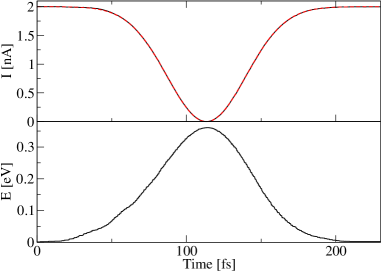
Figure 1: Target current $P(t)$ (dashed) and calculated current $I(t)$ (solid) in the upper panel. The control field $E(t)$ is shown in the lower panel.

As a first simple example of current control we consider a case in which the current is initially constant and the goal is to suppress the current following a Gaussian shape in time. In Fig. 1 the current target $P(t)$ is shown together with the obtained current and the corresponding laser field $E(t)$. Until the initial time $t_{0}$ = 0 the laser field is turned off and the system is equilibrated, i.e. in a steady state leading to a time-independent current. As can be seen the optimal control current matches the target very well. The optimal laser field is slightly asymmetric and its maximum occurs a few femtoseconds before the minimum of the current. This is in agreement with the earlier observation klei06b ; li07a that a Gaussian shaped envelope of the laser field leads to a slightly asymmetric current pattern with a minimum delayed by a few femtoseconds.

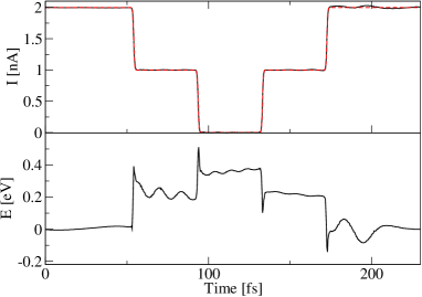
Figure 2: Same as in Fig. 1 for a different control target.

In the second example the complexity of the control task is increased. As shown in Fig. 2 the current target $P(t)$ is a symmetric double step function and the goal is achieved by the optimal control algorithm rather accurately. Only at the last step there is some visible deviation between target and achieved current. The optimized laser field in the lower panel of Fig. 2 also shows step-like features but additionally oscillations and peaks. In contrast to the previous control target, the rapidly changing target current pattern requires larger changes in the electric field. To compensate the effect of these large peaks on the current at later times, additional oscillations of the field are needed to achieve constant values of the current at the plateaus.

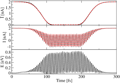
Figure 3: A control target including a highly oscillating pattern. The control target (dashed) and the achieved current (solid) are displayed in the middle panel while in the top panel an average over five oscillatory periods is shown. The control field is given in the lowest part of the figure.

In many experimental setups the laser field has a high carrier frequency and a more slowly varying envelope function. To mimic such a scenario we created a target for the current which consists of a fast oscillating pattern with $\omega=1$ eV modulated by a slowly varying envelope function, namely a current depletion of half-Gaussian form, a constant part, and again a half-Gaussian shape for the increasing current. This pattern together with the current achieved by the optimal control algorithm is shown in the middle panel of Fig. 3. Despite the rapidly varying target function the goal is accurately achieved. Similar to previous studies of CDT we also calculated a mean current which is determined by averaging the current over a few cycles of the carrier frequency, here 5 periods. This procedure can of course be performed for the target as well as for the shaped current and the results are shown in the top panel of Fig. 3. As can be seen the average current is suppressed nicely in such a scenario.

In previous studies lehm03a ; klei06b ; li07a CDT was utilized to suppress the current which is possible for certain values of the amplitude $A$ of the laser field: The fraction $A/\omega$ has to be equal to a zero of the zeroth-order Bessel function. In the present case the maximal value of the field is about $A/\omega=0.8$ which is certainly far off a zero of the zeroth-order Bessel function. Therefore the present current depletion cannot be explained by CDT.

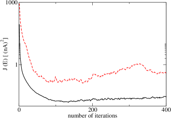
Figure 4: The value of the control function $J(E)$. Solid for the step function as shown in Fig. 2 and dashed for the symmetric Gaussian shape in Fig. 3.

The convergence of the iterative control algorithm for the second and third example is displayed in Fig. 4. It shows how the value of $J$ decreases with increasing number of iterations. For a simple target like a step function, $J$ decreases very fast and then gets more or less constant. In contrast for a complex target with a fast oscillating function, it decreases not so fast in the beginning and later even increases slightly. To further decrease the control function one could increase the Langrange parameter $\lambda$ for large iteration numbers.

In conclusion, we have demonstrated that it is theoretically possible to achieve a time-dependent pattern of the current through a molecular junction. The optimized current can be obtained using an optimal control field. Although we used a simplified model for a molecular wire the present investigation shows that it is worthwhile to study the combination of molecular wires and optimal control theory on the femtosecond time scale, theoretically as well as experimentally. In experiment feedback coherent control for complex systems has been successful brix03 so that an experimental implementation of the ideas described above might be feasible in the future.

The authors would like to thank the Deutsche Forschungsgemeinschaft for financial support within SPP 1243.

References

- (1) A. Nitzan and M. A. Ratner, Science 300, 1384 (2003).
- (2) A. W. Ghosh, P. S. Damle, S. Datta, and A. Nitzan, MRS Bull. 6, 391 (2004).
- (3) M. Büttiker, Phys. Rev. Lett. 57, 1761 (1986).
- (4) Y. Meir and N. S. Wingreen, Phys. Rev. Lett. 68, 2512 (1992).
- (5) N. S. Wingreen, A.-P. Jauho, and Y. Meir, Phys. Rev. B 48, 8487 (1993).
- (6) S. Kohler, J. Lehmann, and P. Hänggi, Phys. Rep. 406, 379 (2005).
- (7) X. Q. Li et al., Phys. Rev. B 71, 205304 (2005).
- (8) P. Cui, X.-Q. Li, J. Shao, and Y. J. Yan, Phys. Lett. A 357, 449 (2006).
- (9) I. V. Ovchinnikov and D. Neuhauser, J. Chem. Phys. 122, 024707 (2005).
- (10) S. Welack, M. Schreiber, and U. Kleinekathöfer, J. Chem. Phys. 124, 044712 (2006).
- (11) U. Harbola, M. Esposito, and S. Mukamel, Phys. Rev. B 74, 235309 (2006).
- (12) J. Lehmann, S. Kohler, P. Hänggi, and A. Nitzan, Phys. Rev. Lett. 88, 228305 (2002).
- (13) A. Tikhonov, R. D. Coalson, and Y. Dahnovsky, J. Chem. Phys. 117, 567 (2002).
- (14) J. Lehmann, S. Camalet, S. Kohler, and P. Hänggi, Chem. Phys. Lett. 368, 282 (2003).
- (15) C. Meier and D. J. Tannor, J. Chem. Phys. 111, 3365 (1999).
- (16) F. Grossmann, T. Dittrich, P. Jung, and P. Hänggi, Phys. Rev. Lett. 67, 516 (1991).
- (17) U. Kleinekathöfer, G.-Q. Li, S. Welack, and M. Schreiber, Europhys. Lett. 75, 139 (2006).
- (18) G.-Q. Li, M. Schreiber, and U. Kleinekathöfer, EPL 79, 27006 (2007).
- (19) A. Kaiser and V. May, J. Chem. Phys. 121, 2528 (2004).
- (20) A. Kaiser and V. May, Chem. Phys. Lett. 405, 339 (2005).
- (21) I. Serban, J. Werschnik, and E. K. U. Gross, Phys. Rev. A 71, 053810 (2005).
- (22) A. Kaiser and V. May, Chem. Phys. 320, 95 (2006).
- (23) C. P. Koch, J. P. Palao, R. Kosloff, and F. Masnou-Seeuws, Phys. Rev. A 70, 013402 (2004).
- (24) J. P. Palao and R. Kosloff, Phys. Rev. A 68, 062308 (2003).
- (25) R. Xu, Y. J. Yan, Y. Ohtsuki, and Y. Fujimura, J. Chem. Phys. 120, 6600 (2004).
- (26) T. Brixner and G. Gerber, ChemPhysChem 4, 418 (2003).