Phase field model of interfaces in single-component systems derived from classical density functional theory

Abstract

Phase field models have been applied in recent years to grain boundaries in single-component systems. The models are based on the minimization of a free energy functional, which is constructed phenomenologically rather than being derived from first principles. In single-component systems the free energy is a functional of a “phase field”, which is an order parameter often referred to as the crystallinity in the context of grain boundaries, but with no precise definition as to what that term means physically. We present a derivation of the phase field model by Allen and Cahn from classical density functional theory first for crystal-liquid interfaces and then for grain boundaries. The derivation provides a clear physical interpretation of the phase field, and it sheds light on the parameters and the underlying approximations and limitations of the theory. We suggest how phase field models may be improved.

I Introduction

The classical density functional theory (DFT) advanced by Haymet and Oxtoby Haymet and Oxtoby (1981); Oxtoby and Haymet (1982) was developed to describe crystal-liquid interfaces. In this paper we will show how this theory may be approximated in a transparent way to derive phase field models of crystal-liquid and grain boundary interfaces in single-component systems. We will also discuss how classical DFT may be applied to grain boundaries in single-component systems. At specified temperature and chemical potential, atoms at the boundary are free to rearrange themselves to accommodate a fixed change of crystal orientation on either side of the boundary. In principle DFT provides an exact treatment of these defects at the atomic level within a grand canonical ensemble. The application of DFT to grain boundaries is of considerable interest in itself as an alternative to grand canonical Monte Carlo simulations and molecular dynamics simulations.

Grain boundaries in single-component systems have been modeled using phase field approaches, most recently by Carter and coworkers Kobayashi et al. (2000); Tang et al. (2006) and Nestler and Wheeler Nestler and Wheeler (2002). All of these studies make use of an Allen-Cahn type free energy functional, obtained in the case of Carter et al. after first integrating out an “orientation field”. These models are based on the minimization of a free energy, which is constructed phenomenologically, referring to symmetries, relevant physical parameters, effective interactions etc., rather than being derived from first principles. The free energy is a functional of a “phase field”, which is an order parameter often referred to as the “crystallinity” in the context of grain boundaries. The crystallinity is interpreted as a measure of the local degree of structural order, but with no attempt to define it more precisely.

Our aim in this paper is to derive a phase field model for crystal-liquid interfaces and grain boundaries in single-component systems from classical density functional theory, providing not only a clear physical interpretation of the phase field, but also an exposition of the various approximations along the way. The mapping also enables us to identify limitations of phase field modeling of interfaces, and to suggest how it may be improved.

We begin by outlining classical DFT and its application by Haymet and Oxtoby to crystal-liquid interfaces, noting key assumptions. While this derivation focuses on a thermodynamic self-consistency equation, applying the same procedure directly to the grand potential leads to the Allen-Cahn equation and subsequently to a phase field model for grain boundaries recently introduced by Carter et al.. Kobayashi et al. (2000). An interesting by-product of the derivation of a phase field model for grain boundaries is the result that the energy and width of a boundary are both predicted to be reduced when there is a short common vector in the reciprocal lattices of both crystals.

II Classical density functional theory

Following an integration over the momentum degrees of freedom, the canonical partition sumHansen and McDonald (2006) in $d$ dimensions for $N$ identical classical particles at positions $\mathbf{r}_{1},\ldots,\mathbf{r}_{N}\in\Omega$, where $\Omega$ is an arbitrarily large volume, interacting via a potential $V_{N}(\mathbf{r}_{1},\ldots,\mathbf{r}_{\mathbf{n}})$ in an external potential $U(\mathbf{r})$ is

$$Z_{N}=\frac{1}{N!}\Lambda^{-dN}\int_{\Omega}\!\!d^{d}\mathrm{r}_{1}\ldots d^{d}\mathrm{r}_{N}\ \exp\left(-\beta\big{(}V_{N}(\mathbf{r}_{1},\ldots,\mathbf{r}_{\mathbf{n}})+\sum_{i=1}^{N}U(\mathbf{r}_{i})\big{)}\right),$$ (1)

where

$$\Lambda=\left(\frac{\beta h^{2}}{2m\pi}\right)^{1/2}$$ (2)

is the de Broglie thermal wave length. The Laplace transform of the canonical partition sum is the grand canonical partition sum

$$\mathcal{Z}=\sum_{N=0}^{\infty}e^{\beta\mu N}Z_{N}\ .$$ (3)

This suggests the introduction of the dimensionless one-body local potential, not to be confused with the effective one-particle potential introduced later:

$$u(\mathbf{r})=\beta\mu-\beta U(\mathbf{r}).$$ (4)

The dimensionless grand potential, $\mathcal{W}=\mathcal{W}[u]=-\ln\mathcal{Z}$, is then a functional of the local potential $u$ only, apart from the implicit dependence on the interaction potential, and the temperature which is assumed to be constant.

Introducing an operator $\hat{\rho}_{N}(\mathbf{r};\mathbf{r}_{1},\ldots,\mathbf{r}_{\mathbf{n}})=\sum_{i}\delta(\mathbf{r}-\mathbf{r}_{i})$ reveals that the particle density, which is the ensemble average $\left\langle\cdot\right\rangle\!$ of this operator, is given by functional differentiation of the grand potential with respect to the local potential

$$\rho([u];\mathbf{r})=\left\langle\hat{\rho}_{N}(\mathbf{r};\mathbf{r}_{1},\ldots,\mathbf{r}_{\mathbf{n}})\right\rangle\!=-\frac{\delta\mathcal{W}[u]}{\delta u(\mathbf{r})}.$$ (5)

This can be seen by rewriting $\beta\mu N-\beta\sum_{i=1}^{N}U(\mathbf{r}_{i})$ as $\int_{\Omega}\mathchoice{\!\!\mathrm{d}^{d}r\,}{\!\mathrm{d}^{d}r\,}{\!\mathrm{d}^{d}r\,}{\!\mathrm{d}^{d}r\,}u(\mathbf{r})\hat{\rho}_{N}(\mathbf{r};\ldots)$ in the grand canonical partition sum.

Taking a Legendre transform, the free energy

$$\mathcal{F}[\rho]=\mathcal{W}[u]+\int_{\Omega}\mathchoice{\!\!\mathrm{d}^{d}r^{\prime}\,}{\!\mathrm{d}^{d}r^{\prime}\,}{\!\mathrm{d}^{d}r^{\prime}\,}{\!\mathrm{d}^{d}r^{\prime}\,}\rho(\mathbf{r}^{\prime})u(\mathbf{r}^{\prime})$$ (6)

produces the conjugates of the cumulants of the density, in particular

$$u(\mathbf{r})=u([\rho];\mathbf{r})=\frac{\delta}{\delta\rho(\mathbf{r})}\mathcal{F}[\rho].$$ (7)

The free energy of an ideal, i.e. non-interacting system, where $V_{N}\equiv 0$, can be integrated,

$$\mathcal{F}_{\text{\tiny id.}}[\rho]=\int_{\Omega}\mathchoice{\!\!\mathrm{d}^{d}r\,}{\!\mathrm{d}^{d}r\,}{\!\mathrm{d}^{d}r\,}{\!\mathrm{d}^{d}r\,}\rho(\mathbf{r})\left(\ln(\Lambda^{d}\rho(\mathbf{r}))-1\right)$$ (8)

and immediately gives rise to the barometric formula $\rho(\mathbf{r})_{\text{\tiny id.}}=\Lambda^{-d}\exp(u_{\text{\tiny id.}}(\mathbf{r}))$. In an ideal system, the external potential necessary to produce a given density profile is found simply by inverting the barometric formula. For a given density profile $\rho$ observed in an interacting particle system, one can calculate the local potential that would be needed in an ideal system, $u_{\text{\tiny id.}}$, to produce the same density profile. The difference between the local potential, $u$, operating in the interacting system, and the ideal local potential is the effective one particle potential $C([\rho];\mathbf{r})$, defined as

$$C([\rho];\mathbf{r})=u_{\text{\tiny id.}}([\rho];\mathbf{r})-u([\rho];\mathbf{r})=\ln(\Lambda^{d}\rho(\mathbf{r}))-u([\rho];\mathbf{r}).$$ (9)

In other words, an ideal system with local potential $u+C$ has the same density profile $\rho$ as the interacting system with local potential $u$.

Similarly, one defines the excess free energy

$$-\Phi[\rho]=\mathcal{F}[\rho]-\mathcal{F}_{\text{\tiny id.}}[\rho],$$ (10)

and finds by differentiation

$$\frac{\delta}{\delta\rho(\mathbf{r})}\Phi[\rho]=C([\rho];\mathbf{r}).$$ (11)

Further differentiation of the effective one-particle potential produces higher order correlation functions. In particular, the direct correlation function $C^{(2)}([\rho];\mathbf{r},\mathbf{r}^{\prime})$ is defined as

$$C^{(2)}([\rho];\mathbf{r},\mathbf{r}^{\prime})\equiv\frac{\delta^{2}}{\delta\rho(\mathbf{r})\delta\rho(\mathbf{r}^{\prime})}\Phi[\rho]\ .$$ (12)

Eq. (12) immediately suggests an expansion of the excess free energy about a reference state, which in the following will be the infinite homogeneous liquid with constant density $\rho_{0}$,

$$\Phi[\rho]=\Phi[\rho\equiv\rho_{0}]+\int_{\Omega}\mathchoice{\!\!\mathrm{d}^{d}r\,}{\!\mathrm{d}^{d}r\,}{\!\mathrm{d}^{d}r\,}{\!\mathrm{d}^{d}r\,}C([\rho\equiv\rho_{0}];\mathbf{r})(\rho(\mathbf{r})-\rho_{0})+\frac{1}{2}\int_{\Omega}\mathchoice{\!\!\mathrm{d}^{d}r\,}{\!\mathrm{d}^{d}r\,}{\!\mathrm{d}^{d}r\,}{\!\mathrm{d}^{d}r\,}\;\mathchoice{\!\!\mathrm{d}^{d}r^{\prime}\,}{\!\mathrm{d}^{d}r^{\prime}\,}{\!\mathrm{d}^{d}r^{\prime}\,}{\!\mathrm{d}^{d}r^{\prime}\,}C^{(2)}([\rho\equiv\rho_{0}];\mathbf{r},\mathbf{r}^{\prime})(\rho(\mathbf{r})-\rho_{0})(\rho(\mathbf{r}^{\prime})-\rho_{0})+\ldots$$ (13)

We use this expansion below to derive features of the crystal phase from the reference system.

Using the Ornstein-Zernike equation Hansen and McDonald (2006) the Fourier transform $c(\mathbf{k})$ of the two-point direct correlation function over a domain with volume $V^{\prime\prime}$ in a translationally invariant system, see Eq. (23), can be directly related to the structure factor $S(\mathbf{k})$

$$S(\mathbf{k})=\left(1-\rho_{0}V^{\prime\prime}c(\mathbf{k})\right)^{-1}\ ,$$ (14)

so that the direct correlation function has a direct physical and experimental meaning. It is, in fact, the only link to experiment, which raises the question of how it is possible that a perturbation theory about a liquid can describe features of a crystal. For example, one might doubt that the tetrahedral structure of crystalline silicon could be predicted from the two point direct correlation function of liquid silicon, which has an average coordination number of $6$. On the other hand, the functional $C^{(2)}([\rho];\mathbf{r},\mathbf{r}^{\prime})$, i.e. the direct correlation function including its functional dependence on the density within the entire system, contains all information about higher order correlations through functional differentiation. In Eq. (13) $C^{(2)}$ is evaluated only at $\rho(\mathbf{r})\equiv\rho_{0}$, so the full functional dependence is suppressed. A key assumption of the theory is that by a judicious choice of $\rho_{0}$ the expansion in Eq. (13) can be made acceptable. This debate has appeared prominently in the literature Ramakrishnan and Yussouff (1979). On a more technical level, the functional Taylor series Eq. (13) may have a finite “radius of convergence” in $\rho(\mathbf{r})-\rho_{0}$, not extending beyond the liquid phase, not least because a phase transition introduces singularities.

III Application to interfaces

In all that follows the approximations are based on the two point direct correlation function $C^{(2)}([\rho\equiv\rho_{0}];\mathbf{r},\mathbf{r}^{\prime})$, which is a function only of the separation $|\mathbf{r}-\mathbf{r}^{\prime}|$ in a homogeneous system. To ease notation, the homogeneous, infinite reference liquid will be denoted by subscript $0$, instead of explicitly carrying the argument $\rho\equiv\rho_{0}$. In this notation, the one-particle potential of the reference system, which is assumed to be homogeneous and to have vanishing local potential $u(\mathbf{r})\equiv u_{0}=\beta\mu$, is related to its density by

$$C_{0}=\ln(\Lambda^{d}\rho_{0})-\beta\mu$$ (15)

consistent with Eq. (9).

We use the reference system to calculate features of an interfacial system (distinguished by subscript $i$) for a given local potential $u_{i}(\mathbf{r})$, which amounts to finding a root $\rho_{i}(\mathbf{r})$ of $u_{i}=\delta\mathcal{F}_{i}[\rho]/\delta\rho$. Equivalently one can minimize the functional

$$\widetilde{\mathcal{W}}([\rho],[u_{i}])=\mathcal{F}_{i}[\rho]-\int_{\Omega}\mathchoice{\!\!\mathrm{d}^{d}r\,}{\!\mathrm{d}^{d}r\,}{\!\mathrm{d}^{d}r\,}{\!\mathrm{d}^{d}r\,}u_{i}(\mathbf{r})\rho(\mathbf{r})$$ (16)

with respect to $\rho$. At the minimum $\rho\equiv\rho_{i}$ and $\widetilde{\mathcal{W}}([\rho_{i}],[u_{i}])$ reduces to the grand potential, as seen in Eq. (6). For a vanishing local potential in the interfacial system $u_{i}\equiv\beta\mu$. The expansion in Eq. (13) together with Eq. (15), Eq. (8) and Eq. (10), is the starting point for the DFT used by Haymet and Oxtoby Haymet and Oxtoby (1981):

$$\widetilde{\mathcal{W}}([\rho_{i}],[u_{i}\equiv\beta\mu]) = \int_{\Omega}\mathchoice{\!\!\mathrm{d}^{d}r^{\prime}\,}{\!\mathrm{d}^{d}r^{\prime}\,}{\!\mathrm{d}^{d}r^{\prime}\,}{\!\mathrm{d}^{d}r^{\prime}\,}\left[\ln\left(\rho_{i}(\mathbf{r}^{\prime})/\rho_{0}\right)-1\right]\rho_{i}(\mathbf{r}^{\prime})-\Phi_{0}+\int_{\Omega}\mathchoice{\!\!\mathrm{d}^{d}r^{\prime}\,}{\!\mathrm{d}^{d}r^{\prime}\,}{\!\mathrm{d}^{d}r^{\prime}\,}{\!\mathrm{d}^{d}r^{\prime}\,}C_{0}\rho_{0}$$

$$-\frac{1}{2}\int_{\Omega}\mathchoice{\!\!\mathrm{d}^{d}r^{\prime}\,}{\!\mathrm{d}^{d}r^{\prime}\,}{\!\mathrm{d}^{d}r^{\prime}\,}{\!\mathrm{d}^{d}r^{\prime}\,}\!\!\int_{\Omega}\mathchoice{\!\!\mathrm{d}^{d}r^{\prime\prime}\,}{\!\mathrm{d}^{d}r^{\prime\prime}\,}{\!\mathrm{d}^{d}r^{\prime\prime}\,}{\!\mathrm{d}^{d}r^{\prime\prime}\,}C^{(2)}_{0}(|\mathbf{r}^{\prime\prime}-\mathbf{r}^{\prime}|)\left(\rho_{i}(\mathbf{r}^{\prime})-\rho_{0}\right)\left(\rho_{i}(\mathbf{r}^{\prime\prime})-\rho_{0}\right).$$

It is worth stressing that the only approximation made so far is the truncation of the functional Taylor series Eq. (13) at second order.

To derive the results of [Haymet and Oxtoby, 1981; Oxtoby and Haymet, 1982] one requires that $\widetilde{\mathcal{W}}$ differentiated with respect to $\rho_{i}$ vanishes. Using $C^{(2)}_{0}(\mathbf{r})=C^{(2)}_{0}(-\mathbf{r})=C^{(2)}_{0}(|\mathbf{r}|)$ this produces the self-consistency equation

$$0=\ln\rho_{i}(\mathbf{r})/\rho_{0}-\int_{\Omega}\mathchoice{\!\!\mathrm{d}^{d}r^{\prime}\,}{\!\mathrm{d}^{d}r^{\prime}\,}{\!\mathrm{d}^{d}r^{\prime}\,}{\!\mathrm{d}^{d}r^{\prime}\,}C^{(2)}_{0}(|\mathbf{r}-\mathbf{r}^{\prime}|)\left(\rho_{i}(\mathbf{r}^{\prime})-\rho_{0}\right),$$ (18)

which can also be obtained by expanding the effective one particle potential in a functional Taylor series. It is very difficult to find a root $\rho_{i}$ for this equation satisfying particular boundary conditions far from the interface.

Physically, it is very appealing to represent the density in a pseudo-Fourier sum Haymet and Oxtoby (1981); Ramakrishnan and Yussouff (1979)

$$\rho_{i}(\mathbf{r})=\rho_{0}\left(1+\sum_{\mathbf{n}}\mu_{\mathbf{n}}(\mathbf{r})e^{\imath\mathbf{k}_{\mathbf{n}}\mathbf{r}}\right)$$ (19)

with reciprocal lattice vectors $\mathbf{k}_{\mathbf{n}}$ indexed by $\mathbf{n}\in\mathbb{Z}^{d}$. For simplicity we have assumed the crystal has a monatomic basis. In crystals with more than one atom in the basis there will be additional phase factors in the pseudo-Fourier expansion. At a crystal-liquid interface there is only one crystal lattice, but at a grain boundary there is one set of reciprocal lattice vectors for each crystal, and the expansion in Eq. (19) is over the union of reciprocal lattice vectors of the two crystals. In the following derivation we will not make use of any specific properties of $\{\mathbf{k}_{\mathbf{n}}\}$ other than its discreteness and completeness (see Eq. (27)), as well as its orthogonality (see Eq. (24)), which all necessitate a finite Fourier domain, introduced in Eq. (20) as the volume $V$. For grain boundaries it follows that the derivation applies only to cases where a three-dimensional coincidence site lattice (CSL) Sutton and Balluffi (1995) exists with a reasonably small unit cell.

Owing to the spatial dependence of the coefficients $\mu_{\mathbf{n}}(\mathbf{r})$, Eq. (19) is not a true Fourier sum. However, it can accommodate every density $\rho_{i}(\mathbf{r})$, even if the density is not periodic. While the spatial dependence has, a priori, the unfortunate consequence that individual coefficients $\mu_{\mathbf{n}}(\mathbf{r})$ cannot be calculated by projecting $\rho_{i}(\mathbf{r})$ onto the functions $e^{-\imath\mathbf{k}_{\mathbf{n}}\mathbf{r}}$, the spatial dependence of the coefficients can be thought of as a means to separate length scales. The atomic-scale density variations are captured by the exponential $\exp(\imath\mathbf{k}_{\mathbf{n}}\mathbf{r})$, while more gradual changes in density are captured by $\mu_{\mathbf{n}}(\mathbf{r})$. We discuss below how the $\mu_{\mathbf{n}}(\widetilde{\mathbf{r}})$ for different $\widetilde{\mathbf{r}}$ can be obtained by taking a local Fourier integral within a volume $V(\widetilde{\mathbf{r}})$,

$$\mu_{\mathbf{n}}(\widetilde{\mathbf{r}})\rho_{0}=V^{-1}\int_{V(\widetilde{\mathbf{r}})}\!\!\!\mathchoice{\!\!\mathrm{d}^{d}r\,}{\!\mathrm{d}^{d}r\,}{\!\mathrm{d}^{d}r\,}{\!\mathrm{d}^{d}r\,}\rho_{i}(\mathbf{r})e^{-\imath\mathbf{k}_{\mathbf{n}}\mathbf{r}}\quad\text{ for }\quad n\neq 0$$ (20)

and $\rho_{0}(1+\mu_{\mathbf{0}}(\widetilde{\mathbf{r}}))=V^{-1}\int_{V(\widetilde{\mathbf{r}})}\mathchoice{\!\!\mathrm{d}^{d}r\,}{\!\mathrm{d}^{d}r\,}{\!\mathrm{d}^{d}r\,}{\!\mathrm{d}^{d}r\,}\rho_{i}(\mathbf{r})$. Here $V(\widetilde{\mathbf{r}})$ denotes the domain the integral is running over, a parallelepiped of volume $V$ which is a unit cell of the coincidence site lattice or a multiple thereof.

Using the new representation Eq. (19) in the self-consistency equation (18) and expanding the $\mu_{\mathbf{n}}(\mathbf{r}^{\prime})$ about $\mathbf{r}$ gives for Eq. (18)

$$\ln\left(1+\sum_{\mathbf{n}}\mu_{\mathbf{n}}(\mathbf{r})e^{\imath\mathbf{k}_{\mathbf{n}}\mathbf{r}}\right)=V^{\prime\prime}\rho_{0}\sum_{\mathbf{n}}e^{\imath\mathbf{k}_{\mathbf{n}}\mathbf{r}}\left[\mu_{\mathbf{n}}(\mathbf{r})c(\mathbf{k}_{\mathbf{n}})-\imath(\nabla_{\mathbf{r}}\cdot\nabla_{\mathbf{k}})\mu_{\mathbf{n}}(\mathbf{r})c(\mathbf{k}_{\mathbf{n}})-\frac{1}{2}(\nabla_{\mathbf{r}}\cdot\nabla_{\mathbf{k}})^{2}\mu_{\mathbf{n}}(\mathbf{r})c(\mathbf{k}_{\mathbf{n}})+\ldots\right]$$ (21)

where

$$\int_{\Omega}\mathchoice{\!\!\mathrm{d}^{d}r^{\prime}\,}{\!\mathrm{d}^{d}r^{\prime}\,}{\!\mathrm{d}^{d}r^{\prime}\,}{\!\mathrm{d}^{d}r^{\prime}\,}C^{(2)}_{0}(|\mathbf{r}-\mathbf{r}^{\prime}|)e^{-\imath\mathbf{k}(\mathbf{r}-\mathbf{r}^{\prime})}=V^{\prime\prime}c(\mathbf{k})$$ (22)

has been used, based on the definition

$$c(\mathbf{k})=V^{\prime\prime-1}\int_{V^{\prime\prime}}\!\!\mathchoice{\!\!\mathrm{d}^{d}r^{\prime\prime}\,}{\!\mathrm{d}^{d}r^{\prime\prime}\,}{\!\mathrm{d}^{d}r^{\prime\prime}\,}{\!\mathrm{d}^{d}r^{\prime\prime}\,}e^{-\imath\mathbf{k}\mathbf{r}^{\prime\prime}}C^{(2)}_{0}(\mathbf{r}^{\prime\prime})\ .$$ (23)

The central idea is that $V^{\prime\prime}$ is so large that $C^{(2)}$ vanishes outside this volume and that $\Omega$ is sufficiently large that the failure of Eq. (22) due to the shift by $\mathbf{r}$ when writing Eq. (22) as Eq. (23) is negligible.

So far, only two approximations have been made, the functional Taylor series of the excess free energy and the Taylor series for the pseudo-Fourier coefficients $\mu_{\mathbf{n}}$. It is perhaps not surprising that Eq. (21) remains just as intractable as Eq. (18), which becomes obvious by taking a Fourier transform over the domain $V(\widetilde{\mathbf{r}})$ centered at $\widetilde{\mathbf{r}}\in\Omega$ on both sides of Eq. (21):

$$V^{-1}\int_{V(\widetilde{\mathbf{r}})}\!\!\!\mathchoice{\!\!\mathrm{d}^{d}r\,}{\!\mathrm{d}^{d}r\,}{\!\mathrm{d}^{d}r\,}{\!\mathrm{d}^{d}r\,}e^{-\imath\mathbf{k}_{\mathbf{m}}\mathbf{r}}\ln\left(1+\sum_{\mathbf{n}}\mu_{\mathbf{n}}(\mathbf{r})e^{\imath\mathbf{k}_{\mathbf{n}}\mathbf{r}}\right)=\\ V^{-1}\int_{V(\widetilde{\mathbf{r}})}\!\!\!\mathchoice{\!\!\mathrm{d}^{d}r\,}{\!\mathrm{d}^{d}r\,}{\!\mathrm{d}^{d}r\,}{\!\mathrm{d}^{d}r\,}e^{-\imath\mathbf{k}_{\mathbf{m}}\mathbf{r}}V^{\prime\prime}\rho_{0}\sum_{\mathbf{n}}e^{\imath\mathbf{k}_{\mathbf{n}}\mathbf{r}}\left[\mu_{\mathbf{n}}(\mathbf{r})c(\mathbf{k}_{\mathbf{n}})-\imath(\nabla_{\mathbf{r}}\cdot\nabla_{\mathbf{k}})\mu_{\mathbf{n}}(\mathbf{r})c(\mathbf{k}_{\mathbf{n}})-\frac{1}{2}(\nabla_{\mathbf{r}}\cdot\nabla_{\mathbf{k}})^{2}\mu_{\mathbf{n}}(\mathbf{r})c(\mathbf{k}_{\mathbf{n}})+\ldots\right].$$ (24)

The problem is the $\mathbf{r}$-dependence of the coefficients $\mu_{\mathbf{n}}(\mathbf{r})$ which renders the orthogonality of the exponentials on the right hand side unexploitable. On the other hand, the representation in Eq. (19) has not yet been fully exploited, in particular, no use has been made so far of the many degrees of freedom in the parametrization.

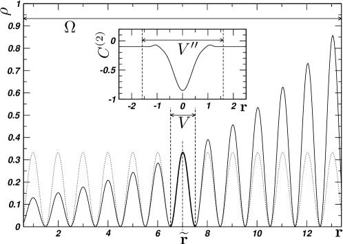
Figure 1: Cartoon of a local Fourier transform. The full line shows the actual density profile $\rho(\mathbf{r})$ within a system of size $\Omega$ parameterized by an expression like Eq. (19) which contains a space dependent pseudo-Fourier coefficient. A Fourier transform taken over the small region $V$ marked by the dashed lines around $\widetilde{\mathbf{r}}$, produces coefficients that reproduce the density locally (shown as thick line) and can be continued periodically throughout the system (dotted line). The inset shows the two point direct correlation function $C^{(2)}(\mathbf{r})$ which drops to a negligible value outside the domain $V^{\prime\prime}$.

Haymet and Oxtoby achieved a separation of length scales by utilizing the parametrization Eq. (19). Firstly, they introduced a family of density profiles indexed by $\widetilde{\mathbf{r}}$,

$$\rho(\mathbf{r};\widetilde{\mathbf{r}})=\rho_{0}\left(1+\sum_{\mathbf{n}}\mu_{\mathbf{n}}(\widetilde{\mathbf{r}})e^{\imath\mathbf{k}_{\mathbf{n}}\mathbf{r}}\right)\ ,$$ (25)

which coincides with Eq. (19) for $\widetilde{\mathbf{r}}=\mathbf{r}$. Secondly, they replace $\mu_{\mathbf{n}}(\mathbf{r})$ by $\mu_{\mathbf{n}}(\widetilde{\mathbf{r}})$ in Eq. (21), requiring that the $\mu_{\mathbf{n}}(\widetilde{\mathbf{r}})$ at fixed $\widetilde{\mathbf{r}}$ are solutions of a slightly different problem,

$$\ln\left(1+\sum_{\mathbf{n}}\mu_{\mathbf{n}}(\widetilde{\mathbf{r}})e^{\imath\mathbf{k}_{\mathbf{n}}\mathbf{r}}\right)=V^{\prime\prime}\rho_{0}\sum_{\mathbf{n}}e^{\imath\mathbf{k}_{\mathbf{n}}\mathbf{r}}\left[\mu_{\mathbf{n}}(\widetilde{\mathbf{r}})c(\mathbf{k}_{\mathbf{n}})-\imath(\nabla_{\mathbf{r}}\cdot\nabla_{\mathbf{k}})\mu_{\mathbf{n}}(\widetilde{\mathbf{r}})c(\mathbf{k}_{\mathbf{n}})-\frac{1}{2}(\nabla_{\mathbf{r}}\cdot\nabla_{\mathbf{k}})^{2}\mu_{\mathbf{n}}(\widetilde{\mathbf{r}})c(\mathbf{k}_{\mathbf{n}})+\ldots\right],$$ (26)

and therefore

$$V^{-1}\int_{V(\widetilde{\mathbf{r}})}\!\!\!\mathchoice{\!\!\mathrm{d}^{d}r\,}{\!\mathrm{d}^{d}r\,}{\!\mathrm{d}^{d}r\,}{\!\mathrm{d}^{d}r\,}e^{-\imath\mathbf{k}_{\mathbf{m}}\mathbf{r}}\ln\left(1+\sum_{\mathbf{n}}\mu_{\mathbf{n}}(\widetilde{\mathbf{r}})e^{\imath\mathbf{k}_{\mathbf{n}}\mathbf{r}}\right)=\\ V^{-1}\int_{V(\widetilde{\mathbf{r}})}\!\!\!\mathchoice{\!\!\mathrm{d}^{d}r\,}{\!\mathrm{d}^{d}r\,}{\!\mathrm{d}^{d}r\,}{\!\mathrm{d}^{d}r\,}e^{-\imath\mathbf{k}_{\mathbf{m}}\mathbf{r}}V^{\prime\prime}\rho_{0}\sum_{\mathbf{n}}e^{\imath\mathbf{k}_{\mathbf{n}}\mathbf{r}}\left[\mu_{\mathbf{n}}(\widetilde{\mathbf{r}})c(\mathbf{k}_{\mathbf{n}})-\imath(\nabla_{\mathbf{r}}\cdot\nabla_{\mathbf{k}})\mu_{\mathbf{n}}(\widetilde{\mathbf{r}})c(\mathbf{k}_{\mathbf{n}})-\frac{1}{2}(\nabla_{\mathbf{r}}\cdot\nabla_{\mathbf{k}})^{2}\mu_{\mathbf{n}}(\widetilde{\mathbf{r}})c(\mathbf{k}_{\mathbf{n}})+\ldots\right]\\ =V^{\prime\prime}\rho_{0}\left[\mu_{\mathbf{m}}(\widetilde{\mathbf{r}})c(\mathbf{k}_{\mathbf{m}})-\imath(\nabla_{\mathbf{r}}\cdot\nabla_{\mathbf{k}})\mu_{\mathbf{m}}(\widetilde{\mathbf{r}})c(\mathbf{k}_{\mathbf{m}})-\frac{1}{2}(\nabla_{\mathbf{r}}\cdot\nabla_{\mathbf{k}})^{2}\mu_{\mathbf{m}}(\widetilde{\mathbf{r}})c(\mathbf{k}_{\mathbf{m}})+\ldots\right],$$ (27)

corresponding to Eq. (24). For a complete, discrete set of reciprocal lattice vectors $\{\mathbf{k}_{\mathbf{n}}\}$ Eq. (27) is equivalent to Eq. (26); in other words, Eq. (26) is implied by Eq. (27) only if (27) applies to the entire set of reciprocal lattice vectors.

The solutions of Eq. (27) for each fixed $\widetilde{\mathbf{r}}$ are periodic density profiles (see Fig. 1) of systems in a certain periodic external potential and it is plausible to assume that solutions in the form $\mu_{\mathbf{n}}(\widetilde{\mathbf{r}})$ exist. Moreover, Eq. (26) evaluated at $\widetilde{\mathbf{r}}=\mathbf{r}$ coincides with Eq. (21), so that any set of solutions of Eq. (27) also represents a solution of Eq. (24). In other words, Haymet and Oxtoby construct a family of physical systems parameterized by $\widetilde{\mathbf{r}}$ in an external potential, the density profiles of which are given by $\mu_{\mathbf{n}}(\widetilde{\mathbf{r}})$ and can be used to construct a solution of the interfacial problem Eq. (24) by evaluating Eq. (25) at $\widetilde{\mathbf{r}}=\mathbf{r}$.

Because Eq. (27) can also be obtained by assuming in Eq. (24) the $\mu_{\mathbf{n}}(\mathbf{r})$ vary so little within $V(\widetilde{\mathbf{r}})$ they can be replaced by $\mu_{\mathbf{n}}(\widetilde{\mathbf{r}})$ (see Eq. (20)), going from Eq. (24) to Eq. (27) is equivalent to a separation of length scales. This separation of length scales validates Eq. (20). It is illustrated in Fig. 1, where the Fourier coefficient $\mu_{\mathbf{n}}(\widetilde{\mathbf{r}})$ obtained by taking a Fourier integral over a small domain centered at $\widetilde{\mathbf{r}}$, gives rise to a density profile that can be periodically continued throughout the system, but coincides almost perfectly with the actual density $\rho_{i}(\mathbf{r})$ within $V(\widetilde{\mathbf{r}})$.

Small $V$ are desirable so that the separation of length scales as encapsulated in Eq. (20) applies with no or only small corrections. For a grain boundary, the volume $V$ is a unit cell of the CSL, so that large $\Sigma$ boundaries are expected to be less reliably treated. Similarly, small $V^{\prime\prime}$ are desirable so that the expansion in Eq. (21) has only small corrections, which implies that shorter-ranged direct correlation functions are easier to handle in this formalism. The size of both volumes is to be compared to the scale on which $\mu_{\mathbf{n}}(\mathbf{r})$ change.

We see in Eq. (27) that the separation of length scales embodied in Eq. (25) simplifies the original equation (24) dramatically by enabling the orthogonality of the functions $\exp(\imath\mathbf{k}_{\mathbf{n}}\mathbf{r})$ to be exploited. Instead of finding roots $\mu_{\mathbf{n}}(\mathbf{r})$ for all $\mathbf{k}_{\mathbf{n}}$ and all $\mathbf{r}\in\Omega$ of the original integral equation Eq. (24) simultaneously, the integro-differential equation Eq. (27) can in principle be integrated, as both sides are local in $\widetilde{\mathbf{r}}$. As shown in ref. [Oxtoby and Haymet, 1982], the $\mu_{\mathbf{n}}(\mathbf{r})$ can be considered positions of particles in a (complicated) potential at “time” $\mathbf{r}$ projected on the interface normal. In DFT, the next steps would consist in determining the necessary degrees of freedom, incorporating all symmetries and prescribing a procedure to find the roots $\mu_{\mathbf{n}}(\widetilde{\mathbf{r}})$ for every $\mathbf{n}$ and $\widetilde{\mathbf{r}}$.

IV Derivation of phase field models

IV.1 Crystal-liquid interfaces

We will now build on the approximations, expansions and parameterizations described in the previous section to derive an Allen-Cahn phase field model for crystal-liquid interfaces from the grand-potential Eq. (III). In the next sub-section we will derive a phase field model for grain boundaries.

The grand potential $\widetilde{\mathcal{W}}$ in the form Eq. (III) is reparameterized using Eq. (19) and the integrals over $\Omega$ rewritten as $\int_{\Omega}\mathchoice{\!\!\mathrm{d}^{d}r^{\prime}\,}{\!\mathrm{d}^{d}r^{\prime}\,}{\!\mathrm{d}^{d}r^{\prime}\,}{\!\mathrm{d}^{d}r^{\prime}\,}=\int_{\Omega}\mathchoice{\!\!\mathrm{d}^{d}\widetilde{r}\,}{\!\mathrm{d}^{d}\widetilde{r}\,}{\!\mathrm{d}^{d}\widetilde{r}\,}{\!\mathrm{d}^{d}\widetilde{r}\,}V^{-1}\!\!\int_{V(\widetilde{\mathbf{r}})}\mathchoice{\!\!\mathrm{d}^{d}r^{\prime}\,}{\!\mathrm{d}^{d}r^{\prime}\,}{\!\mathrm{d}^{d}r^{\prime}\,}{\!\mathrm{d}^{d}r^{\prime}\,}$:

$$\widetilde{\mathcal{W}}([\rho_{i}],[u_{i}\equiv\beta\mu]) = \int_{\Omega}\mathchoice{\!\!\mathrm{d}^{d}\widetilde{r}\,}{\!\mathrm{d}^{d}\widetilde{r}\,}{\!\mathrm{d}^{d}\widetilde{r}\,}{\!\mathrm{d}^{d}\widetilde{r}\,}V^{-1}\!\!\!\int_{V(\widetilde{\mathbf{r}})}\!\mathchoice{\!\!\mathrm{d}^{d}r^{\prime}\,}{\!\mathrm{d}^{d}r^{\prime}\,}{\!\mathrm{d}^{d}r^{\prime}\,}{\!\mathrm{d}^{d}r^{\prime}\,}\left(\ln\left(1+\sum_{\mathbf{n}}\mu_{\mathbf{n}}(\mathbf{r}^{\prime})e^{\imath\mathbf{k}_{\mathbf{n}}\mathbf{r}^{\prime}}\right)-1\right)\rho_{0}\left(1+\sum_{\mathbf{n}}\mu_{\mathbf{n}}(\mathbf{r}^{\prime})e^{\imath\mathbf{k}_{\mathbf{n}}\mathbf{r}^{\prime}}\right)-\Phi_{0}$$

$$+\int_{\Omega}\mathchoice{\!\!\mathrm{d}^{d}r^{\prime}\,}{\!\mathrm{d}^{d}r^{\prime}\,}{\!\mathrm{d}^{d}r^{\prime}\,}{\!\mathrm{d}^{d}r^{\prime}\,}C_{0}\rho_{0}-\frac{1}{2}\rho_{0}^{2}\int_{\Omega}\mathchoice{\!\!\mathrm{d}^{d}\widetilde{r}\,}{\!\mathrm{d}^{d}\widetilde{r}\,}{\!\mathrm{d}^{d}\widetilde{r}\,}{\!\mathrm{d}^{d}\widetilde{r}\,}\ V^{-1}\!\!\!\int_{V(\widetilde{\mathbf{r}})}\!\mathchoice{\!\!\mathrm{d}^{d}r^{\prime}\,}{\!\mathrm{d}^{d}r^{\prime}\,}{\!\mathrm{d}^{d}r^{\prime}\,}{\!\mathrm{d}^{d}r^{\prime}\,}\int_{\Omega}\mathchoice{\!\!\mathrm{d}^{d}r^{\prime\prime}\,}{\!\mathrm{d}^{d}r^{\prime\prime}\,}{\!\mathrm{d}^{d}r^{\prime\prime}\,}{\!\mathrm{d}^{d}r^{\prime\prime}\,}C^{(2)}_{0}(\mathbf{r}^{\prime\prime}-\mathbf{r}^{\prime})\sum_{\mathbf{n}\mathbf{m}}\mu_{\mathbf{n}}(\mathbf{r}^{\prime})\mu_{\mathbf{m}}(\mathbf{r}^{\prime\prime})e^{\imath(\mathbf{k}_{\mathbf{n}}\mathbf{r}^{\prime}+\mathbf{k}_{\mathbf{m}}\mathbf{r}^{\prime\prime})}$$

As in the calculation of the Fourier coefficients of $C^{(2)}$, see Eq. (23), the equality between the single integral over $\Omega$ and the double integral over individual volumes $V(\widetilde{\mathbf{r}})$ centered at $\widetilde{\mathbf{r}}$ ignores surface terms and holds only in the limit of infinite or periodic $\Omega$, because the volume $V(\widetilde{\mathbf{r}})$ at a point $\widetilde{\mathbf{r}}$ close to the surface of $\Omega$ might not be fully within $\Omega$. After expanding the coefficients $\mu_{\mathbf{m}}(\mathbf{r}^{\prime\prime})$ about $\mathbf{r}^{\prime}$ and using the definition Eq. (23) (in the notation $\nabla_{k}c(-\mathbf{k}_{\mathbf{m}})=\nabla_{k}|_{-\mathbf{k}_{\mathbf{m}}}c(\mathbf{k})$ and noting that $c(-\mathbf{k})=c(\mathbf{k})$ etc. ) the last triple integral becomes

$$V^{\prime\prime}\int_{\Omega}\mathchoice{\!\!\mathrm{d}^{d}\widetilde{r}\,}{\!\mathrm{d}^{d}\widetilde{r}\,}{\!\mathrm{d}^{d}\widetilde{r}\,}{\!\mathrm{d}^{d}\widetilde{r}\,}V^{-1}\!\!\!\int_{V(\widetilde{\mathbf{r}})}\!\mathchoice{\!\!\mathrm{d}^{d}r^{\prime}\,}{\!\mathrm{d}^{d}r^{\prime}\,}{\!\mathrm{d}^{d}r^{\prime}\,}{\!\mathrm{d}^{d}r^{\prime}\,}\sum_{\mathbf{n}\mathbf{m}}\mu_{\mathbf{n}}(\mathbf{r}^{\prime})\left[\mu_{\mathbf{m}}(\mathbf{r}^{\prime})c(\mathbf{k}_{\mathbf{m}})-\imath(\nabla_{\mathbf{r}}\cdot\nabla_{\mathbf{k}})\mu_{\mathbf{m}}(\mathbf{r}^{\prime})c(\mathbf{k}_{\mathbf{m}})-\frac{1}{2}(\nabla_{\mathbf{r}}\cdot\nabla_{\mathbf{k}})^{2}\mu_{\mathbf{m}}(\mathbf{r}^{\prime})c(\mathbf{k}_{\mathbf{m}})+\ldots\right]e^{\imath(\mathbf{k}_{\mathbf{n}}+\mathbf{k}_{\mathbf{m}})\mathbf{r}^{\prime}}$$ (29)

which is very similar to the right-hand side of Eq. (21). Assuming a perfect separation of length scales, so that the $\mu_{\mathbf{n}}(\mathbf{r}^{\prime})$ do not change within the volume of a unit cell $V$, allows us to replace $\mu_{\mathbf{n}}(\mathbf{r}^{\prime})$ by $\mu_{\mathbf{n}}(\widetilde{\mathbf{r}})$ within the integrals over $V(\widetilde{\mathbf{r}})$ and to make use of the orthogonality of the exponentials, so that $\widetilde{\mathcal{W}}$ becomes

$$\widetilde{\mathcal{W}}([\rho_{i}],[u_{i}\equiv\beta\mu])$$

$$= \int_{\Omega}\mathchoice{\!\!\mathrm{d}^{d}\widetilde{r}\,}{\!\mathrm{d}^{d}\widetilde{r}\,}{\!\mathrm{d}^{d}\widetilde{r}\,}{\!\mathrm{d}^{d}\widetilde{r}\,}V^{-1}\!\!\!\int_{V(\widetilde{\mathbf{r}})}\!\mathchoice{\!\!\mathrm{d}^{d}r^{\prime}\,}{\!\mathrm{d}^{d}r^{\prime}\,}{\!\mathrm{d}^{d}r^{\prime}\,}{\!\mathrm{d}^{d}r^{\prime}\,}\left(\ln\left(1+\sum_{\mathbf{n}}\mu_{\mathbf{n}}(\widetilde{\mathbf{r}})e^{\imath\mathbf{k}_{\mathbf{n}}\mathbf{r}^{\prime}}\right)-1\right)\rho_{0}\left(1+\sum_{\mathbf{n}}\mu_{\mathbf{n}}(\widetilde{\mathbf{r}})e^{\imath\mathbf{k}_{\mathbf{n}}\mathbf{r}^{\prime}}\right)$$

$$-\Phi_{0}+\int_{\Omega}\mathchoice{\!\!\mathrm{d}^{d}r^{\prime}\,}{\!\mathrm{d}^{d}r^{\prime}\,}{\!\mathrm{d}^{d}r^{\prime}\,}{\!\mathrm{d}^{d}r^{\prime}\,}C_{0}\rho_{0}$$

$$-\frac{1}{2}\rho_{0}^{2}V^{\prime\prime}\int_{\Omega}\mathchoice{\!\!\mathrm{d}^{d}\widetilde{r}\,}{\!\mathrm{d}^{d}\widetilde{r}\,}{\!\mathrm{d}^{d}\widetilde{r}\,}{\!\mathrm{d}^{d}\widetilde{r}\,}\sum_{\mathbf{n}}\mu_{-\mathbf{n}}(\widetilde{\mathbf{r}})\left[\mu_{\mathbf{n}}(\widetilde{\mathbf{r}})c(\mathbf{k}_{\mathbf{n}})-\imath(\nabla_{\mathbf{r}}\cdot\nabla_{\mathbf{k}})\mu_{\mathbf{n}}(\widetilde{\mathbf{r}})c(\mathbf{k}_{\mathbf{n}})-\frac{1}{2}(\nabla_{\mathbf{r}}\cdot\nabla_{\mathbf{k}})^{2}\mu_{\mathbf{n}}(\widetilde{\mathbf{r}})c(\mathbf{k}_{\mathbf{n}})+\ldots\right]$$

This is the final result for the grand potential. Differentiating with respect to $\mu_{-\mathbf{j}}(\widehat{\mathbf{r}})$ gives

$$\frac{\delta}{\delta\mu_{-\mathbf{j}}(\widehat{\mathbf{r}})}\widetilde{\mathcal{W}}([\rho_{i}],[u_{i}\equiv\beta\mu]) = V^{-1}\int_{V(\widehat{\mathbf{r}})}\mathchoice{\!\!\mathrm{d}^{d}r^{\prime}\,}{\!\mathrm{d}^{d}r^{\prime}\,}{\!\mathrm{d}^{d}r^{\prime}\,}{\!\mathrm{d}^{d}r^{\prime}\,}\rho_{0}e^{\imath\mathbf{k}_{-\mathbf{j}}\mathbf{r}^{\prime}}\ln\left(1+\sum_{\mathbf{n}}\mu_{\mathbf{n}}(\widehat{\mathbf{r}})e^{\imath\mathbf{k}_{\mathbf{n}}\mathbf{r}^{\prime}}\right)$$

$$-\rho_{0}^{2}V^{\prime\prime}\left[\mu_{\mathbf{j}}(\widehat{\mathbf{r}})c(\mathbf{k}_{\mathbf{j}})-\imath(\nabla_{\mathbf{r}}\cdot\nabla_{\mathbf{k}})\mu_{\mathbf{j}}(\widehat{\mathbf{r}})c(\mathbf{k}_{\mathbf{j}})-\frac{1}{2}(\nabla_{\mathbf{r}}\cdot\nabla_{\mathbf{k}})^{2}\mu_{\mathbf{j}}(\widehat{\mathbf{r}})c(\mathbf{k}_{\mathbf{j}})+\ldots\right]$$

using, again, $c(\mathbf{k}_{\mathbf{j}})=c(\mathbf{k}_{-\mathbf{j}})$, $\nabla_{k}c(\mathbf{k}_{\mathbf{j}})=-\nabla_{k}c(\mathbf{k}_{-\mathbf{j}})$ etc. and $\mathbf{k}_{-\mathbf{j}}=-\mathbf{k}_{\mathbf{j}}$. Moreover, we made use of

$$\frac{\delta}{\delta f(x)}\int\mathchoice{\!\!\mathrm{d}y\,}{\!\mathrm{d}y\,}{\!\mathrm{d}y\,}{\!\mathrm{d}y\,}f^{\prime}(y)g(y)=-g^{\prime}(x)$$ (32)

which is obtained by ignoring surface term in an integration by parts. This is particularly important when trying to include into a functional the first derivatives, $\nabla_{\mathbf{r}}\mu_{\mathbf{n}}(\mathbf{r})$, reminiscent of a Rayleigh friction term in a mechanical interpretation.

Eq. (IV.1) is to be compared to Eq. (27), the original result by Haymet and Oxtoby, which is reproduced by Eq. (IV.1) by requiring $\frac{\delta}{\delta\mu_{-\mathbf{j}}(\widehat{\mathbf{r}})}\widetilde{\mathcal{W}}\equiv 0$. The time evolution of $\mu_{\mathbf{j}}(\widehat{\mathbf{r}})$ is usually set equal to that derivative,

$$\dot{\mu}_{\mathbf{j}}(\widehat{\mathbf{r}})=-M\frac{\delta}{\delta\mu_{\mathbf{j}}(\widehat{\mathbf{r}})}\widetilde{\mathcal{W}}$$ (33)

with mobility $M$ (which can be absorbed into the definition of time), driving the system to the above mentioned root. This is precisely the mechanism used in many phase field models.

Further simplifications are needed to write the grand potential Eq. (IV.1) in Allen-Cahn form. The set of independent amplitudes $\mu_{\mathbf{n}}(\widetilde{\mathbf{r}})$ is replaced by a single scaling amplitude $\phi(\widetilde{\mathbf{r}})$ by writing

$$\mu_{\mathbf{n}}(\widetilde{\mathbf{r}})=\phi(\widetilde{\mathbf{r}})\mu^{0}_{\mathbf{n}}$$ (34)

with constant amplitudes $\mu^{0}_{\mathbf{n}}$ chosen to represent a crystalline phase, so that $\phi(\widetilde{\mathbf{r}})=1$ corresponds to the crystalline phase, while $\phi(\widetilde{\mathbf{r}})=0$ suppresses all structure, corresponding to a liquid with density $\rho_{0}$. The field $\phi$ therefore is to be interpreted as the order parameter, proportional to the local amplitude of the atomic density waves, i.e. $\phi$ is the crystallinity. The common amplitude $\phi(\widetilde{\mathbf{r}})$ is necessarily real, because $\rho$ being real implies $\mu_{\mathbf{n}}(\mathbf{r})^{*}=\mu_{-\mathbf{n}}(\mathbf{r})$ and together with $\mu_{\mathbf{n}}^{0*}=\mu_{-\mathbf{n}}^{0}$ (see below) we therefore have $\phi(\widetilde{\mathbf{r}})^{*}=\phi(\widetilde{\mathbf{r}})$.

Collecting all local contributions in the density $w(\phi(\mathbf{r}))$, the grand potential Eq. (IV.1) simplifies to

$$\widetilde{\mathcal{W}}([\phi]) = \int_{\Omega}\mathchoice{\!\!\mathrm{d}^{d}r\,}{\!\mathrm{d}^{d}r\,}{\!\mathrm{d}^{d}r\,}{\!\mathrm{d}^{d}r\,}w(\phi(\mathbf{r}))$$

$$+\frac{1}{2}\rho_{0}^{2}V^{\prime\prime}\int_{\Omega}\mathchoice{\!\!\mathrm{d}^{d}\widetilde{r}\,}{\!\mathrm{d}^{d}\widetilde{r}\,}{\!\mathrm{d}^{d}\widetilde{r}\,}{\!\mathrm{d}^{d}\widetilde{r}\,}\sum_{\mathbf{n}}\phi(\widetilde{\mathbf{r}})\mu^{0}_{-\mathbf{n}}\left[\imath(\nabla_{\mathbf{r}}\cdot\nabla_{\mathbf{k}})\phi(\widetilde{\mathbf{r}})\mu^{0}_{\mathbf{n}}c(\mathbf{k}_{\mathbf{n}})+\frac{1}{2}(\nabla_{\mathbf{r}}\cdot\nabla_{\mathbf{k}})^{2}\phi(\widetilde{\mathbf{r}})\mu^{0}_{\mathbf{n}}c(\mathbf{k}_{\mathbf{n}})\right]$$

which can be simplified further by ignoring the surface terms of the integral $\int\mathchoice{\!\!\mathrm{d}^{d}\widetilde{r}\,}{\!\mathrm{d}^{d}\widetilde{r}\,}{\!\mathrm{d}^{d}\widetilde{r}\,}{\!\mathrm{d}^{d}\widetilde{r}\,}\phi(\widetilde{\mathbf{r}})\nabla_{\mathbf{r}}\phi(\widetilde{\mathbf{r}})$ so that the remaining integral containing derivatives of $\phi(\mathbf{r})$ has the structure

$$\int_{\Omega}\mathchoice{\!\!\mathrm{d}^{d}\widetilde{r}\,}{\!\mathrm{d}^{d}\widetilde{r}\,}{\!\mathrm{d}^{d}\widetilde{r}\,}{\!\mathrm{d}^{d}\widetilde{r}\,}\phi(\widetilde{\mathbf{r}})\sum_{\mathbf{n}}\mu^{0}_{-\mathbf{n}}\mu^{0}_{\mathbf{n}}(\nabla_{\mathbf{r}}\cdot\nabla_{\mathbf{k}})^{2}\phi(\widetilde{\mathbf{r}})c(\mathbf{k}_{\mathbf{n}})\ .$$ (36)

To simplify this expression, the set of reciprocal lattice vectors $\mathbf{k}_{\mathbf{n}}$ in the sum must be reduced. We use the index $\mathbf{n}^{0}$ to indicate that we are considering only a subset $\{\mathbf{k}_{\mathbf{n}^{0}}\}$ of all possible reciprocal lattice vectors $\{\mathbf{k}_{\mathbf{n}}\}$. In the simplest approximation, the set is reduced to the set comprising only the shortest (non-vanishing) reciprocal lattice vectors, $\{\mathbf{k}_{\mathbf{n}^{0}}\}$. This set $\{\mathbf{k}_{\mathbf{n}^{0}}\}$ forms a “star” which means that elements of this set are related by point symmetry operations of the reciprocal lattice (for further details see the Appendix, Subsection LABEL:sec:stars), so that the star is invariant under these operations. If the real-space lattice is FCC, for example, the reciprocal lattice is BCC and the eight nearest neighbor reciprocal lattice vectors $1\,1\,1$, $\overline{1}\,1\,1$, …, $\overline{1}\,\overline{1}\,\overline{1}$ form the star of shortest length vectors. By including only the shortest reciprocal lattice vectors the symmetry and lattice constant of the crystalline structure are described correctly by the truncated Fourier expansion. The approximation can be systematically improved by including stars of longer reciprocal lattice vectors.

Symmetry requires that all coefficients $\mu^{0}_{\mathbf{n}^{0}}$ as introduced in Eq. (34) associated with any of the vectors $\mathbf{k}_{\mathbf{n}^{0}}$ within the same star have equal magnitude. Inversion symmetry in the real-space lattice ensures that $\mu^{0}_{-\mathbf{n}^{0}}=\mu^{0}_{\mathbf{n}^{0}}$, if we impose that the center of inversion coincides with a site. Since $\mu^{0*}_{\mathbf{n}^{0}}=\mu^{0}_{-\mathbf{n}^{0}}$ by reality of $\rho$, all $\mu^{0}_{\mathbf{n}^{0}}$ are real and therefore equal, $\mu^{0}_{\mathbf{n}^{0}}=\mu_{0}$. It is this equality which is needed to simplify Eq. (36), by allowing us to place $\mu^{0}_{-\mathbf{n}}\mu^{0}_{\mathbf{n}}$ in front of the remaining sum, which is dealt with in the following.

The direct correlation function of the bulk liquid is isotropic, $c(\mathbf{k})=\tilde{c}(|\mathbf{k}|)$, so that the second derivative with respect to wave-vector components $1\leq\alpha\leq d$ and $1\leq\beta\leq d$ in Eq. (36) can be written as

$$\partial_{k_{\alpha}}\partial_{k_{\beta}}c(\mathbf{k})=\frac{\delta_{\alpha\beta}}{|\mathbf{k}|}\tilde{c}^{\prime}(|\mathbf{k}|)-\frac{k_{\alpha}k_{\beta}}{|\mathbf{k}|^{3}}\tilde{c}^{\prime}(|\mathbf{k}|)+\frac{k_{\alpha}k_{\beta}}{|\mathbf{k}|^{2}}\tilde{c}^{\prime\prime}(|\mathbf{k}|)\ .$$ (37)

In a sum of the form

$$\sum_{\mathbf{k}_{\mathbf{n}^{0}}}(\nabla_{\mathbf{r}}\cdot\nabla_{\mathbf{k}})^{2}\phi(\widetilde{\mathbf{r}})c(\mathbf{k}_{\mathbf{n}^{0}})=\sum_{\mathbf{k}_{\mathbf{n}^{0}}}\sum_{\alpha=1}^{d}\sum_{\beta=1}^{d}\partial_{k_{\alpha}}\partial_{k_{\beta}}\partial_{\widetilde{x}_{\alpha}}\partial_{\widetilde{x}_{\beta}}\phi(\widetilde{\mathbf{r}})c(\mathbf{k}_{\mathbf{n}^{0}})\\ =\sum_{\mathbf{k}_{\mathbf{n}^{0}}}\sum_{\alpha,\beta}^{d}\left(\frac{\delta_{\alpha\beta}}{|\mathbf{k}_{\mathbf{n}^{0}}|}\tilde{c}^{\prime}(|\mathbf{k}_{\mathbf{n}^{0}}|)-\frac{k_{\mathbf{n}^{0},\alpha}k_{\mathbf{n}^{0},\beta}}{|\mathbf{k}_{\mathbf{n}^{0}}|^{3}}\tilde{c}^{\prime}(|\mathbf{k}_{\mathbf{n}^{0}}|)+\frac{k_{\mathbf{n}^{0},\alpha}k_{\mathbf{n}^{0},\beta}}{|\mathbf{k}_{\mathbf{n}^{0}}|^{2}}\tilde{c}^{\prime\prime}(|\mathbf{k}_{\mathbf{n}^{0}}|)\right)\partial_{\widetilde{x}_{\alpha}}\partial_{\widetilde{x}_{\beta}}\phi(\widetilde{\mathbf{r}})\ ,$$ (38)

where the $\mathbf{k}_{\mathbf{n}^{0}}$ run over all elements of the star $\{\mathbf{k}_{\mathbf{n}^{0}}\}$, the contributions of off-diagonal elements, $\alpha\neq\beta$, vanish after taking the summation over the star $\mathbf{k}_{\mathbf{n}^{0}}$, if one assumes a cubic crystal system. Only the diagonal elements remain and by symmetry each Cartesian component contributes $\sum_{\{\mathbf{k}_{\mathbf{n}^{0}}\}}k_{\alpha}^{2}=(q/d)|\mathbf{k}|^{2}$, where $q=|\{\mathbf{k}_{\mathbf{n}^{0}}\}|$ is the cardinality of the star, i.e. the number of elements in $\{\mathbf{k}_{\mathbf{n}^{0}}\}$. The dimension $d$ is the dimension of the space spanned by the star. For example, the $8$ nearest neighbors in a BCC lattice (the reciprocal lattice of an FCC lattice) would have $q=8$ and $d=3$.

The proof of this simplification is based on the Great Orthogonality Theorem of group theory Inui et al. (1996) as detailed in the Appendix. The assumption of cubic symmetry ensures that there is always a three-dimensional, unitary, irreducible representation of the point group. The assumption can be lifted if one allows for anisotropic terms (see the Appendix, Subsection LABEL:sec:stars), reflecting the anisotropy of the lattice. In the following, we consider only cubic crystal systems.

The sum in the integrand of Eq. (36) now becomes

$$\sum_{\mathbf{k}_{\mathbf{n}^{0}}}\phi(\widetilde{\mathbf{r}})\mu^{0}_{-\mathbf{n}^{0}}(\nabla_{\mathbf{r}}\cdot\nabla_{\mathbf{k}})^{2}\phi(\widetilde{\mathbf{r}})\mu^{0}_{\mathbf{n}^{0}}c(\mathbf{k}_{\mathbf{n}^{0}}) = \left(\frac{q(d-1)}{|\mathbf{k}_{0}|d}\tilde{c}^{\prime}(|\mathbf{k}_{0}|)+\frac{q}{d}\tilde{c}^{\prime\prime}(|\mathbf{k}_{0}|)\right)\mu_{0}^{2}\phi(\widetilde{\mathbf{r}})\nabla_{\mathbf{r}}^{2}\phi(\widetilde{\mathbf{r}})$$

$$= -\epsilon_{\mathbf{k}_{0}}\phi(\widetilde{\mathbf{r}})\nabla_{\mathbf{r}}^{2}\phi(\widetilde{\mathbf{r}})\ ,$$

where we have used $|\mathbf{k}_{0}|$ to denote the magnitude of any member of the star $\{\mathbf{k}_{\mathbf{n}^{0}}\}$, and we have introduced the coupling $\epsilon_{\mathbf{k}_{0}}$ defined as

$$\epsilon_{\mathbf{k}_{0}}=-\left(\frac{q(d-1)}{|\mathbf{k}_{0}|d}\tilde{c}^{\prime}(|\mathbf{k}_{0}|)+\frac{q}{d}\tilde{c}^{\prime\prime}(|\mathbf{k}_{0}|)\right)\mu_{0}^{2}\ .$$ (40)

The expression for $\epsilon_{\mathbf{k}_{0}}$ simplifies further because the structure factor Eq. (14) usually peaks at the shortest reciprocal lattice vectorRamakrishnan and Yussouff (1979), so that $\tilde{c}^{\prime}$ vanishes and $\tilde{c}^{\prime\prime}<0$. In that case

$$\epsilon_{\mathbf{k}_{0}}=\frac{q}{d}|\tilde{c}^{\prime\prime}(|\mathbf{k}_{0}|)|\mu_{0}^{2}\ .$$ (41)

which enters the grand potential Eq. (IV.1) as follows

$$\widetilde{\mathcal{W}}_{\text{AC}}([\phi])=\int_{\Omega}\mathchoice{\!\!\mathrm{d}^{d}r\,}{\!\mathrm{d}^{d}r\,}{\!\mathrm{d}^{d}r\,}{\!\mathrm{d}^{d}r\,}\left(w(\phi(\mathbf{r}))+\frac{1}{4}\rho_{0}^{2}V^{\prime\prime}\epsilon_{\mathbf{k}_{0}}\left(\nabla_{\mathbf{r}}\phi(\mathbf{r})\right)^{2}\ \right)\ ,$$ (42)

ignoring surface contributions again. Functional differentiation of Eq. (42) with respect to the phase field $\phi(\mathbf{r})$ then reproduces the Allen-Cahn equation Boettinger et al. (2002)

$$\dot{\phi}=-M\left(\frac{dw}{d\phi}-\frac{1}{2}\rho_{0}^{2}V^{\prime\prime}\frac{g}{d}|\tilde{c}^{\prime\prime}(|\mathbf{k}_{0}|)|\mu_{0}^{2}\nabla_{\mathbf{r}}^{2}\phi(\mathbf{r})\right)$$ (43)

in which the relaxational assumption

$$\frac{\delta}{\delta\phi}\widetilde{\mathcal{W}}=-M\frac{d}{dt}\phi\ ,$$

(with mobility $M$) has been made to drive $\widetilde{\mathcal{W}}[\phi]$ to a minimum with respect to $\phi$.

The above analysis may be improved by including more stars of reciprocal lattice vectors than just the shortest. Indeed, the entire reciprocal lattice can be decomposed into disjoint stars without double-counting. The sum over more than one star $\{\mathbf{k}_{\mathbf{n}^{0}}\}$ produces an effective coupling

$$\epsilon=\sum_{\{\mathbf{k}_{\mathbf{n}^{0}}\}}\epsilon_{\mathbf{k}_{\mathbf{n}^{0}}}$$ (44)

replacing $\epsilon_{\mathbf{k}_{0}}$ in Eq. (42).

IV.2 Grain boundaries

As noted in Section LABEL:sec:App_to_Ints we confine ourselves to misorientations where there is a CSL with a relatively small three-dimensional unit cell to ensure that the finite Fourier domain $V(\mathbf{r})$ in the separation of length scales (see Eq. (20)) does not lead to significant errors. In practice this limits the treatment to grain boundaries in cubic lattices, where such CSLs arise frequently.

In the simplest treatment of a grain boundary we consider one set of shortest length reciprocal lattice vectors in each crystal, which we call $\mathbb{S}_{l}=\{\mathbf{k}^{l}_{\mathbf{n}^{0}}\}$ and $\mathbb{S}_{r}=\{\mathbf{k}^{r}_{\mathbf{n}^{0}}\}$ for the left and right crystals respectively. Again, both these sets form stars, see Appendix, Subsection LABEL:sec:stars, and they are related by the rotation that generates the misorientation in the bicrystal. The atomic densities deep in the left and right crystals are described by density waves with wave vectors that are elements of these stars, and with equal amplitudes $\mu^{l}_{\mathbf{n}^{0}}=\mu^{l}_{0}$ and $\mu^{r}_{\mathbf{n}^{0}}=\mu^{r}_{0}$ respectively, similar to the situation in the crystal-liquid interface. That does not mean, however, that all wave-vectors have non-zero amplitudes: For example, if a wave-vector in the right star is not also member of the left star, then its amplitude $\mu^{l}_{\mathbf{n}^{0}}$ vanishes identically by symmetry. Amplitudes are non-zero and equal within the respective stars. Again, it is this equality that is used in the following to simplify the expressions.

In the spirit of Eq. (34), we approximate the spatial dependence of the amplitudes $\{\mu_{\mathbf{n}^{0}}(\widetilde{\mathbf{r}})\}$ by introducing a phase field $\phi(\widetilde{\mathbf{r}})$ for the grain boundary in the form

$$\mu_{\mathbf{n}^{0}}(\widetilde{\mathbf{r}})=\left(1-\phi(\widetilde{\mathbf{r}})\right)\mu^{l}_{\mathbf{n}^{0}}+\phi(\widetilde{\mathbf{r}})\mu^{r}_{\mathbf{n}^{0}}\ .$$ (45)

To satisfy the boundary conditions far from the boundary plane $\phi(\widetilde{\mathbf{r}})$ must vary from $0$ deep in the left-hand crystal to $1$ deep in the right-hand crystal. But this form of $\{\mu_{\mathbf{n}^{0}}(\widetilde{\mathbf{r}})\}$ does not allow for density waves which have non-zero amplitudes only in the grain boundary core, thereby restricting the degrees of freedom available to the system. There is no such restriction in place at the starting point of the derivation, Eq. (IV.1), which included, in principle, all $\mathbf{k}$-vectors of the direct sum of the two stars, i.e. the entire “DSC lattice” Sutton and Balluffi (1995).

At closer inspection, the parameterization (45) of $\mu_{\mathbf{n}^{0}}(\widetilde{\mathbf{r}})$ makes a slightly different use of the “crystallinity” $\phi(\widetilde{\mathbf{r}})$, as it forces the system to be, on average, a superposition of both crystalline lattices: As one is gradually “switched off”, the other is gradually “switched on”, so that $\phi(\widetilde{\mathbf{r}})$ is the crystallinity of the right lattice and $1-\phi(\widetilde{\mathbf{r}})$ is the crystallinity of the left lattice. Reciprocal lattice vectors common to both lattices are predicted by Eq. (45) to be constant throughout the bicrystal, if $\mu_{0}^{l}=\mu_{0}^{r}$. Even if $\mu_{0}^{l}\neq\mu_{0}^{r}$ the parameterization (45) disallows the possibility of a disordered grain boundary structure where all the $\{\mu_{\mathbf{n}^{0}}(\widetilde{\mathbf{r}})\}$ are locally zero. To resolve this problem, an alternative form of Eq. (45) is needed, for example $\mu_{\mathbf{n}^{0}}=(1/2)\phi\left((1+\phi)\mu^{l}_{\mathbf{n}^{0}}+(1-\phi)\mu^{r}_{\mathbf{n}^{0}}\right)$ with $\phi$ varying from $-1$ to $1$. Yet, by continuity such a form would force the grain boundary to be disordered somewhere Tang et al. (2006). In the following, we will use Eq. (45), which leads to the Allen-Cahn equation in a natural way.

To see how the two different stars enter, the following derivation is presented in some detail. Inserting Eq. (45) in Eq. (IV.1) produces the sum

$$\sum_{\mathbf{k}_{\mathbf{n}^{0}}}\left[\left(1-\phi(\widetilde{\mathbf{r}})\right)\mu^{l}_{\mathbf{n}^{0}}+\phi(\widetilde{\mathbf{r}})\mu^{r}_{\mathbf{n}^{0}}\right]\left(\nabla_{\mathbf{r}}\cdot\nabla_{\mathbf{k}}\right)^{2}\left[\left(1-\phi(\widetilde{\mathbf{r}})\right)\mu^{l}_{\mathbf{n}^{0}}+\phi(\widetilde{\mathbf{r}})\mu^{r}_{\mathbf{n}^{0}}\right]c(\mathbf{k}_{\mathbf{n}}^{0})$$ (46)

which can be rewritten as four sums,

$$\begin{array}[]{rlrll}&\sum_{\mathbf{k}_{\mathbf{n}^{0}}}&\left(1-\phi\right)\mu^{l}_{\mathbf{n}^{0}}&\left(\nabla_{\mathbf{r}}\cdot\nabla_{\mathbf{k}}\right)^{2}&\left(1-\phi\right)\mu^{l}_{\mathbf{n}^{0}}\\ +&\sum_{\mathbf{k}_{\mathbf{n}^{0}}}&\left(1-\phi\right)\mu^{l}_{\mathbf{n}^{0}}&\left(\nabla_{\mathbf{r}}\cdot\nabla_{\mathbf{k}}\right)^{2}&\phi\mu^{r}_{\mathbf{n}^{0}}\\ +&\sum_{\mathbf{k}_{\mathbf{n}^{0}}}&\phi\mu^{r}_{\mathbf{n}^{0}}&\left(\nabla_{\mathbf{r}}\cdot\nabla_{\mathbf{k}}\right)^{2}&\left(1-\phi\right)\mu^{l}_{\mathbf{n}^{0}}\\ +&\sum_{\mathbf{k}_{\mathbf{n}^{0}}}&\phi\mu^{r}_{\mathbf{n}^{0}}&\left(\nabla_{\mathbf{r}}\cdot\nabla_{\mathbf{k}}\right)^{2}&\phi\mu^{r}_{\mathbf{n}^{0}}\ .\end{array}$$ (47)

In the grand potential these sums are integrated over all space, see Eq. (36). A term of the form $\phi(\nabla_{\mathbf{r}}\cdot\nabla_{\mathbf{k}})^{2}(1-\phi)$ therefore equals $(1-\phi)(\nabla_{\mathbf{r}}\cdot\nabla_{\mathbf{k}})^{2}\phi$ following integration by parts and ignoring surface terms, which in turn equals $-\phi(\nabla_{\mathbf{r}}\cdot\nabla_{\mathbf{k}})^{2}\phi$ after ignoring surface terms again. The first sum in (47), for example, then reads

$$\begin{array}[]{rlrll}&\sum_{\mathbf{k}_{\mathbf{n}^{0}}}&\left(1-\phi\right)\mu^{l}_{\mathbf{n}^{0}}&\left(\nabla_{\mathbf{r}}\cdot\nabla_{\mathbf{k}}\right)^{2}&\left(1-\phi\right)\mu^{l}_{\mathbf{n}^{0}}\\ =&\sum_{\mathbf{k}_{\mathbf{n}^{0}}}&\phi\mu^{l}_{\mathbf{n}^{0}}&\left(\nabla_{\mathbf{r}}\cdot\nabla_{\mathbf{k}}\right)^{2}&\phi\mu^{l}_{\mathbf{n}^{0}}\\ =&\sum_{\mathbb{S}_{l}}&\phi\mu^{l}_{\mathbf{n}^{0}}&\left(\nabla_{\mathbf{r}}\cdot\nabla_{\mathbf{k}}\right)^{2}&\phi\mu^{l}_{\mathbf{n}^{0}}\end{array}$$ (48)

where the last equality is due to the coefficients $\mu^{l}_{\mathbf{n}^{0}}$ vanishing for those $\mathbf{k}$-vectors that are not member of the left star. For those $\mathbf{k}$-vectors that are members, on the other hand, the corresponding coefficients $\mu^{l}_{\mathbf{n}^{0}}$ are all equal to $\mu^{l}_{0}$, which can be placed outside the sum. Applying the same procedure to all four sums in Eq. (47), gives

$$\sum_{\mathbb{S}_{l}\cup\mathbb{S}_{r}}\left[\left(1-\phi(\widetilde{\mathbf{r}})\right)\mu^{l}_{\mathbf{n}^{0}}+\phi(\widetilde{\mathbf{r}})\mu^{r}_{\mathbf{n}^{0}}\right]\left(\nabla_{\mathbf{r}}\cdot\nabla_{\mathbf{k}}\right)^{2}\left[\left(1-\phi(\widetilde{\mathbf{r}})\right)\mu^{l}_{\mathbf{n}^{0}}+\phi(\widetilde{\mathbf{r}})\mu^{r}_{\mathbf{n}^{0}}\right]$$

$$= \ \mu_{0}^{l\,2}\sum_{\mathbb{S}_{l}}\phi(\widetilde{\mathbf{r}})(\nabla_{\mathbf{r}}\cdot\nabla_{\mathbf{k}})^{2}\phi(\widetilde{\mathbf{r}})+\mu_{0}^{r\,2}\sum_{\mathbb{S}_{r}}\phi(\widetilde{\mathbf{r}})(\nabla_{\mathbf{r}}\cdot\nabla_{\mathbf{k}})^{2}\phi(\widetilde{\mathbf{r}})-2\mu_{0}^{l}\mu_{0}^{r}\sum_{\mathbb{I}}\phi(\widetilde{\mathbf{r}})(\nabla_{\mathbf{r}}\cdot\nabla_{\mathbf{k}})^{2}\phi(\widetilde{\mathbf{r}})\ .$$

The intersection $\mathbb{I}=\mathbb{S}_{l}\cap\mathbb{S}_{r}$ contains the reciprocal lattice vectors common to both stars, for which the product $\mu^{l}_{\mathbf{n}^{0}}\mu^{r}_{\mathbf{n}^{0}}$ is non-zero. The intersection is assumed to be itself a star (see the Appendix, Subsection LABEL:sec:stars for details). To Eq. (IV.2) the simplification based on the Great Orthogonality Theorem (see the Appendix) can be applied. Because the space spanned by $\mathbb{I}$ is potentially only a sub-vector vector space of $\mathbb{R}^{d}$, a projection matrix $P_{\mathbb{I}}$ needs to be introduced, which projects any vector of $\mathbb{R}^{d}$ to this sub-vector space. For the cubic systems we are focusing on here, this sub-vector space has either dimension $d_{\mathbb{I}}=0$ in which case $P_{\mathbb{I}}=0$, or $d_{\mathbb{I}}=d$ in which case $P_{\mathbb{I}}=\mathbf{1}$ is the identity matrix, or $d_{\mathbb{I}}=1$ in which case one spatial direction, say $z$, can be chosen to coincide with the common direction. Using the Great Orthogonality Theorem, Eq. (IV.2) becomes

$$\sum_{\mathbb{S}_{l}\cup\mathbb{S}_{r}}\left[\left(1-\phi(\widetilde{\mathbf{r}})\right)\mu^{l}_{\mathbf{n}^{0}}+\phi(\widetilde{\mathbf{r}})\mu^{r}_{\mathbf{n}^{0}}\right]\left(\nabla_{\mathbf{r}}\cdot\nabla_{\mathbf{k}}\right)^{2}\left[\left(1-\phi(\widetilde{\mathbf{r}})\right)\mu^{l}_{\mathbf{n}^{0}}+\phi(\widetilde{\mathbf{r}})\mu^{r}_{\mathbf{n}^{0}}\right]c(\mathbf{k}_{\mathbf{n}^{0}})$$

$$= \ (\mu_{0}^{l\,2}+\mu_{0}^{r\,2})\phi(\widetilde{\mathbf{r}})\left(\frac{q(d-1)}{|\mathbf{k}_{0}|d}\tilde{c}^{\prime}(|\mathbf{k}_{0}|)+\frac{q}{d}\tilde{c}^{\prime\prime}(|\mathbf{k}_{0}|)\right)\nabla_{\mathbf{r}}^{2}\phi(\widetilde{\mathbf{r}})$$ (50)

$$-2\mu_{0}^{l}\mu_{0}^{r}\phi(\widetilde{\mathbf{r}})\left(\frac{q_{\mathbb{I}}}{|\mathbf{k}_{0}|}\tilde{c}^{\prime}(|\mathbf{k}_{0}|)\nabla_{\mathbf{r}}^{2}-\frac{q_{\mathbb{I}}}{|\mathbf{k}_{0}|d_{\mathbb{I}}}\tilde{c}^{\prime}(|\mathbf{k}_{0}|)\nabla_{\mathbf{r}}P_{\mathbb{I}}\nabla_{\mathbf{r}}+\frac{q_{\mathbb{I}}}{d_{\mathbb{I}}}\tilde{c}^{\prime\prime}(|\mathbf{k}_{0}|)\nabla_{\mathbf{r}}P_{\mathbb{I}}\nabla_{\mathbf{r}}\right)\phi(\widetilde{\mathbf{r}})\ ,$$

where the stars $\mathbb{S}_{l}$ and $\mathbb{S}_{r}$ each contain $q$ elements, $\mathbb{I}$ contains $q_{\mathbb{I}}$ elements, and $d_{\mathbb{I}}$ is the dimension of the space spanned by $\mathbb{I}$. The two terms in Eq. (50) have the same prefactor if $\mu_{0}^{l}=\mu_{0}^{r}=\mu_{0}$, which is a physically sensible choice we adopt henceforth.

Suppose there is no misorientation between the crystal lattices. Then there is no grain boundary and Eq. (50) should reduce to zero. With no misorientation we would have $\mathbb{S}_{l}=\mathbb{S}_{r}=\mathbb{I}$, so that $q_{\mathbb{I}}=q$, $d_{\mathbb{I}}=d$ and $P_{\mathbb{I}}=\mathbf{1}$. Substitution of these values into the right hand side of Eq. (50) shows that it does indeed vanish.

We identify in Eq. (50) an isotropic coupling term in which

$$\epsilon_{i}=-2\mu_{0}^{2}\left(\frac{q(d-1)}{|\mathbf{k}_{0}|d}\tilde{c}^{\prime}(|\mathbf{k}_{0}|)+\frac{q}{d}\tilde{c}^{\prime\prime}(|\mathbf{k}_{0}|)\right)+2\mu_{0}^{2}\left(\frac{q_{\mathbb{I}}}{|\mathbf{k}_{0}|}\tilde{c}^{\prime}(|\mathbf{k}_{0}|)\right)$$ (51)

multiplies $-\phi(\widetilde{\mathbf{r}})\nabla_{\mathbf{r}}^{2}\phi(\widetilde{\mathbf{r}})$. There is also an possibly anisotropic coupling term multiplying $-\phi(\widetilde{\mathbf{r}})\nabla_{\mathbf{r}}P_{\mathbb{I}}\nabla_{\mathbf{r}}\phi(\widetilde{\mathbf{r}})$:

$$\epsilon_{a}=2\mu_{0}^{2}\left(-\frac{q_{\mathbb{I}}}{|\mathbf{k}_{0}|d_{\mathbb{I}}}\tilde{c}^{\prime}(|\mathbf{k}_{0}|)+\frac{q_{\mathbb{I}}}{d_{\mathbb{I}}}\tilde{c}^{\prime\prime}(|\mathbf{k}_{0}|)\right)\ .$$ (52)

This last term is not necessarily anisotropic, because for the particular choice of stars, $P_{\mathbb{I}}$ might be $0$ or the identity. In a cubic system, if $P_{\mathbb{I}}$ is non-zero and non-trivial for a given pair of stars, it is equal to any non-zero, non-trivial $P_{\mathbb{I}}$ produced by any other pair of stars. If the approximation is improved by adding further pairs of stars, they will all generate the same types of terms, namely either multiplying $\nabla_{\mathbf{r}}^{2}$ or $\nabla_{\mathbf{r}}P_{\mathbb{I}}\nabla_{\mathbf{r}}$.

The resulting grand potential has again square gradient form

$$\widetilde{\mathcal{W}}_{\text{AC}}([\phi])=\int_{\Omega}\mathchoice{\!\!\mathrm{d}^{d}r\,}{\!\mathrm{d}^{d}r\,}{\!\mathrm{d}^{d}r\,}{\!\mathrm{d}^{d}r\,}\left(w(\phi(\mathbf{r}))+\frac{1}{4}\rho_{0}^{2}V^{\prime\prime}\left(\epsilon_{i}\left(\nabla_{\mathbf{r}}\phi(\mathbf{r})\right)^{2}+\epsilon_{a}\nabla_{\mathbf{r}}\phi(\mathbf{r})P_{\mathbb{I}}\nabla_{\mathbf{r}}\phi(\mathbf{r})\right)\right)\ ,$$ (53)

We note the difference in sign for the two couplings, Eq. (51) and Eq. (52), which becomes most obvious when $\tilde{c}^{\prime}=0$. Thus, we have shown that common reciprocal lattice vectors reduce the square gradient term in the interfacial energy, resulting in a lower interfacial energy and a smaller interfacial width, the characteristic scale of which is given by the coupling $\epsilon_{i}+\epsilon_{a}$, which has the dimension of a length squared. The smaller this coupling, the smaller the penalty for rapid changes in $\phi$. The amount of the reduction by common reciprocal lattice vectors depends on the magnitude of the second derivative $\tilde{c}^{\prime\prime}(|\mathbf{k}_{0}|)$, which decreases with increasing $|\mathbf{k}_{0}|$. Thus the shorter the common reciprocal lattice vectors the larger their influence on the width and energy of the boundary. The influence of common reciprocal lattice vectors on the boundary energy has been known for a long time Sutton and Balluffi (1995), but we are not aware that their influence on the boundary width has been noted before.

V Discussion

In this paper we have shown how the classical density functional theory of Haymet and Oxtoby may be modified to produce an Allen-Cahn type free energy functional first for crystal-liquid interfaces and then for grain boundaries. For both types of interface the phase field is identified with the amplitudes of atomic density waves, providing a physical interpretation of the “crystallinity” of phenomenological phase field models.

Let us consider first the approximations that were required to derive an Allen-Cahn free energy functional from classical density functional theory. To obtain Eq. (21) only two approximations were made. Firstly, the excess free energy functional was expanded and the resulting series was truncated at the second order term, see Eq. (III). Secondly the Taylor series for $\mu_{\mathbf{n}}(\mathbf{r}^{\prime})$ about $\mathbf{r}$ in Eq. (21) was also truncated at the second order term. In principle both these expansions may be taken to higher order terms, although not without a significant increase in complexity. This would be the natural way to extend a phase field model to higher order terms with parameters related to fundamental quantities such as higher order correlation functions.

The key step which lead to equation (IV.1) for the grand potential $\widetilde{\mathcal{W}}$, and eventually to a phase field model, was the separation of length scales. However, this was not an approximation as we discussed after Eq. (27).

The approximations mentioned so far were those of classical density functional theory of crystal-liquid interfaces as implemented by Haymet and Oxtoby. To obtain a phase field model for a crystal-liquid interface two further approximations were necessary. Firstly, the spatial dependence of all $\mu_{\mathbf{n}}(\mathbf{r})$ was assumed to be described by a single field, the “phase field” $\phi(\mathbf{r})$. While classical density functional theory naturally handles a larger set of density waves with independent amplitudes $\mu_{\mathbf{n}}$, phase field modeling in single-component systems to date has considered only a single order parameter, which we have identified as being proportional to the local amplitude of the atomic density waves. The obvious deficiency is the highly restricted nature of the configurational phase space made available to the crystal-liquid interface. When the same approach is adopted for a grain boundary, see Eq. (45), the restrictions are even more severe. Secondly, all $\mu_{\mathbf{n}^{0}}^{l}$ and $\mu_{\mathbf{n}^{0}}^{r}$ within a star are assumed to be identical and real, which suppresses any relative phase factor of the density waves. For example, if there were a rigid translation of one crystal relative to the other on either side of the grain boundary this would lead to complex density wave amplitudes in one crystal. The simplistic assumption made in Eq. (IV.2) eliminates the possibility of any rigid body relative translation.

It is clear that there are quite severe limitations of current phase field models of grain boundaries in single-component systems, at least when they are interpreted in the framework of classical density functional. Can we use DFT to indicate how these phase field models may be improved? We have already seen that going beyond the second order term in the expansion Eq. (III) will introduce higher order correlation functions and hence more information about structure and bonding. Indeed, going to at least third order correlation functions would seem to be necessary in covalent crystals such as silicon. This would introduce higher order terms in the grand potential Eq. (IV.1) and in the Allen-Cahn free energy functional Eq. (42) with parameters that are directly related to the higher order correlation functions. But perhaps the most obvious and pressing improvement would be the introduction of a second independent phase field to describe the amplitudes of two sets of density waves, one for each crystal. Far from the interface the crystal structures are related by a rotation. If we also wish to be able to predict a relative rigid body translation between the crystals, with components parallel and perpendicular to the interface, it will be necessary to allow the density wave amplitudes of one crystal to be complex.

Appendix A Summing over a star

In this Appendix, we derive the equations based on the Great Orthogonality Theorem, as used in Eq. (IV.1) and (50). In particular, we will identify their prerequisites and possible extensions.

The aim is to simplify expressions of the form

$$\sum_{\alpha\beta}\sum_{\mathbf{k}_{\mathbf{n}^{0}}}k_{\mathbf{n}^{0},\alpha}k_{\mathbf{n}^{0},\beta}v_{\alpha}w_{\beta}=\sum_{\alpha\beta}M_{\alpha\beta}v_{\alpha}w_{\beta}$$ (54)

where we may interpret $M_{\alpha\beta}$ as an element of a matrix $M$. Introducing bra and ket notation for convenience the matrix $M$ can be expressed as,

$$\sum_{\mathbf{k}_{\mathbf{n}^{0}}}\left|\mathbf{k}_{\mathbf{n}^{0}}\right\rangle\left\langle\mathbf{k}_{\mathbf{n}^{0}}\right|=M\ .$$ (55)

In Eqns. (54) and (55) the sums run over a set of vectors $\{\mathbf{k}_{\mathbf{n}^{0}}\}\subset\mathbb{R}^{d}$ of equal length, which, for the time being, we will call a “star”. This term will be defined properly in the next section.

The star is picked from the reciprocal lattice, and it is expected to display some point group symmetries of this lattice, in the sense that these point group operations effect only a permutation of members of the star, so that the star itself remains invariant. We assume that the star under consideration is invariant under a group of order $g$, which has a unitary, irreducible representation $\{U_{n}\}$, $n=1,\dots,g$, and that this representation has the same dimension $d$ as the vectors that make up the star. Acting with $U_{n}$ from the left and with $U_{n}^{\dagger}$ from the right on both sides of Eq. (55) merely amounts to a permutation of the summands, because of the invariance of the star. Therefore $M$ commutes with any group element,

$$U_{n}MU_{n}^{\dagger}=M\ ,$$ (56)

so that $\sum_{n}U_{n}MU_{n}^{\dagger}=gM$ and therefore

$$gM_{kl}=\sum_{n}^{g}\sum_{i,j}^{d}(U_{n})_{ki}M_{ij}(U_{n}^{\dagger})_{jl}=(\operatorname{Tr}M)\frac{g}{d}\delta_{kl}$$ (57)

where in the last equality we have used the Great Orthogonality Theorem (for unitary representations),

$$\sum_{n}^{g}(U_{n})_{ki}(U_{n}^{\dagger})_{jl}=\frac{g}{d}\delta_{kl}\delta_{ij}\ .$$ (58)

By construction, the trace $\operatorname{Tr}M$ is the sum over the squares of the moduli of all vectors in the star, which all have the same length, which we call $|\mathbf{k}_{0}|$. So, if the cardinality of the star is $q$, then $\operatorname{Tr}M=q|\mathbf{k}_{0}|^{2}$ and one finally arrives at the general result

$$\sum_{\mathbf{k}_{\mathbf{n}^{0}}}k_{\mathbf{n}^{0},\alpha}k_{\mathbf{n}^{0},\beta}=\frac{q}{d}|\mathbf{k}_{0}|^{2}\delta_{\alpha\beta}$$ (59)

provided there exists a group under which the star is invariant and for which there is a unitary, irreducible representation of the same dimension as the vectors that make up the star.

The fact that the Great Orthogonality Theorem applies only to irreducible representations of the group is a limitation of the above derivation, which motivates the following extension. By construction, the rank of the matrix $M$ is $d$, which is the dimension of the vector space the $\mathbf{k}_{\mathbf{n}^{0}}$ are taken from. A priori, it is unknown whether there exists a group under which the star is invariant and that has an irreducible, unitary representation with dimension $d$. Eq. (59) applies only if a suitable group and a suitable representation exists.

If the star spans a sub vector space of dimension $d^{\prime}$ less than $d$, one cannot expect that it is invariant under a representation with dimension $d$. For example, the star $\mathbb{K}_{1}=\{1\,0\,0,0\,1\,0,\overline{1}\,0\,0,0\,\overline{1}\,0\}$ is not invariant under any irreducible three-dimensional representation of any group, because it will always contain some group elements that will rotate the star out of the $xy$-plane in which all members of the star are located. So, Eq. (59) cannot apply to $\mathbb{K}_{1}$.

On the other hand, considering only the two-dimensional sub vector space spanned by $\mathbb{K}_{1}$ (the $xy$ plane), the star $\mathbb{K}_{2}=\{1\,0,0\,1,\overline{1}\,0,0\,\overline{1}\}$ derived from $\mathbb{K}_{1}$ by appropriate projection, is invariant under some unitary, irreducible representations of $C_{4v}$, some of which have dimension $2$ (and some have dimension $1$). Of course, the original star $\mathbb{K}_{1}$ is also invariant under some three-dimensional representations of $C_{4v}$, but none of them is irreducible.

If a star is contained entirely in a vector space of dimension $d^{\prime}<d$, its members can be expressed in $d$-dimensional space as

$$\left|\mathbf{k}_{\mathbf{n}^{0}}\right\rangle=OB\left|\mathbf{k}^{\prime}_{\mathbf{n}^{0}}\right\rangle\qquad\text{and}\qquad\left\langle\mathbf{k}_{\mathbf{n}^{0}}\right|=\left\langle\mathbf{k}^{\prime}_{\mathbf{n}^{0}}\right|B^{\dagger}O^{\dagger}$$ (60)

where $O$ is an arbitrary rotation matrix of rank $d$, $B$ is a $d\times d^{\prime}$ projection matrix with $B_{ij}=\delta_{ij}$ and $\left|\mathbf{k}^{\prime}_{\mathbf{n}^{0}}\right\rangle$ is a vector in $\mathbb{R}^{d^{\prime}}$. The matrix $B$ increases the number of elements in the vector from $d^{\prime}$ to $d$ and the rotation matrix $O$ rotates the resulting vector to an arbitrary position. The vectors $\{\left|\mathbf{k}^{\prime}_{\mathbf{n}^{0}}\right\rangle\}$ also form a star, now in the sub-vector space $\mathbb{R}^{d^{\prime}}$, so that

$$\sum_{\mathbf{k}^{\prime}_{\mathbf{n}^{0}}}\left|\mathbf{k}^{\prime}_{\mathbf{n}^{0}}\right\rangle\left\langle\mathbf{k}^{\prime}_{\mathbf{n}^{0}}\right|=\frac{q}{d^{\prime}}|\mathbf{k}^{\prime}_{0}|^{2}\mathbf{1}$$ (61)

if there exists a group under which the star $\{\left|\mathbf{k}^{\prime}_{\mathbf{n}^{0}}\right\rangle\}$ is invariant, and which has a (unitary) irreducible representation of dimension $d^{\prime}$. Therefore

$$\sum_{\mathbf{k}_{\mathbf{n}^{0}}}\left|\mathbf{k}_{\mathbf{n}^{0}}\right\rangle\left\langle\mathbf{k}_{\mathbf{n}^{0}}\right|=\frac{q}{d^{\prime}}|\mathbf{k}_{0}|^{2}(OBB^{\dagger}O^{\dagger})$$ (62)

using $|\mathbf{k}_{0}|=|\mathbf{k}^{\prime}_{0}|$ and applying $OB$ on Eq. (61) from the left and $B^{\dagger}O^{\dagger}$ from the right. The matrix $(OBB^{\dagger}O^{\dagger})=P$ (rotate, remove element, rotate back) projects a vector in $R^{d}$ onto the vector space isomorphic to $R^{d^{\prime}}$. For example

$$P=\left(\begin{array}[]{rrr}1&0&0\\ 0&1&0\\ 0&0&0\end{array}\right)$$ (63)

for the star $\mathbb{K}_{1}$ introduced above, using its representation in the $xy$ plane, $\mathbb{K}_{2}$. The construction of the vectors $\mathbf{k}_{\mathbf{n}^{0}}$ from $\mathbf{k}^{\prime}_{\mathbf{n}^{0}}$ in Eq. (60) represents an important limitation: At first sight, Eq. (62) seems to apply to every star that has some degree of symmetry. However, not every star can be written in the form Eq. (60). For example, $\mathbb{K}_{3}=\{1\,0\,1,0\,1\,1,\overline{1}\,0\,1,0\,\overline{1}\,1\}$ has a $C_{4v}$ symmetry, but this star spans the entire $\mathbb{R}^{d}$ and so there is no star $\{\left|\mathbf{k}^{\prime}_{\mathbf{n}^{0}}\right\rangle\}\subset\mathbb{R}^{d^{\prime}}$ that would fulfill Eq. (60) with $d^{\prime}<d$.

In a more compact form, the general result is

$$\sum_{\mathbf{k}_{\mathbf{n}^{0}}}k_{\mathbf{n}^{0},\alpha}k_{\mathbf{n}^{0},\beta}=\frac{q}{d^{\prime}}|\mathbf{k}_{0}|^{2}P_{\alpha\beta}\ ,$$ (64)

provided there exists an unitary, irreducible representation of a group under which the star $\{\left|\mathbf{k}_{\mathbf{n}^{0}}\right\rangle\}\subset\mathbb{R}^{d}$ is invariant, with a dimension $d^{\prime}$ identical to that of the space spanned by the star. Furthermore, if $d^{\prime}=d$, then $P$ reduces to the identity. Eq. (64) can be used in the form

$$\sum_{\alpha\beta}\sum_{\mathbf{k}_{\mathbf{n}^{0}}}k_{\mathbf{n}^{0},\alpha}k_{\mathbf{n}^{0},\beta}\partial_{\widetilde{x}_{\alpha}}\partial_{\widetilde{x}_{\beta}}=\frac{q}{d^{\prime}}|\mathbf{k}_{0}|^{2}\sum_{\alpha\beta}P_{\alpha\beta}\partial_{\widetilde{x}_{\alpha}}\partial_{\widetilde{x}_{\beta}}=\frac{q}{d^{\prime}}|\mathbf{k}_{0}|^{2}\nabla_{\widetilde{x}}P\nabla_{\widetilde{x}}$$ (65)

which leads to Eq. (50).

A.1 Definition of a star

So far in this Appendix a star has been defined as any set of $k$-vectors of equal length. We now adopt the standard definition of a star, which will enforce the conditions required for Eq. (59) or (64) to apply: A star is generated from an initial vector by applying all symmetry operations in the form of a unitary, irreducible representation of the point group of the lattice in the appropriate coordinate system. This representation is chosen so that the lattice itself is invariant under its action, so that the star represents a finite subset of the lattice. The star generated is highly degenerate, giving rise to the so-called “little groups”.

There are two important caveats: Firstly, only cubic crystals have point group symmetries with three-dimensional irreducible representations. Secondly, the intersection of two stars does not necessarily have a irreducible with a dimension equal to that of the space spanned by the intersection. Generally, both points can be addressed in the same way, namely by decomposing stars or the intersection thereof into smaller stars which then have the required properties. But that produces additional projection matrices, so that, for example, the isotropic $\nabla_{\widetilde{\mathbf{r}}}^{2}$ terms in Eq. (IV.1) and (50) split into multiple terms with different projections of the form $\nabla_{\widetilde{\mathbf{r}}}P\nabla_{\widetilde{\mathbf{r}}}$.

All the cubic point groups, and only the cubic point groups, have three-dimensional, unitary, irreducible representations, and the intersection of any two stars generated by one of these representations is either empty, one-dimensional, or it coincides with both stars. For cubic crystals all equations derived above apply without restrictions, producing an isotropic term and a anisotropic one with a single, preferred direction.

References

- Haymet and Oxtoby (1981) A. D. J. Haymet and D. W. Oxtoby, J. Chem. Phys. 74, 2559 (1981).
- Oxtoby and Haymet (1982) D. W. Oxtoby and A. D. J. Haymet, J. Chem. Phys. 76, 6262 (1982).
- Kobayashi et al. (2000) R. Kobayashi, J. A. Warren, and W. C. Carter, Physica D 140, 141 (2000).
- Tang et al. (2006) M. Tang, W. C. Carter, and R. M. Cannon, Phys. Rev. B 73, 024102 (2006).
- Nestler and Wheeler (2002) B. Nestler and A. A. Wheeler, Comp. Phys. Comm. 147, 230 (2002).
- Hansen and McDonald (2006) J.-P. Hansen and I. R. McDonald, Theory of simple liquids (Academic Press, London, UK, 2006).
- Ramakrishnan and Yussouff (1979) T. V. Ramakrishnan and M. Yussouff, Phys. Rev. B 19, 2775 (1979).
- Sutton and Balluffi (1995) A. P. Sutton and R. W. Balluffi, Interfaces in crystalline materials (Oxford University Press, New York, NY, 1995).
- Inui et al. (1996) T. Inui, Y. Tanabe, and Y. Onodera, Group Theory and Its Applications in Physics (Springer-Verlag, Berlin Heidelberg New York, 1996), 2nd ed.
- Boettinger et al. (2002) W. J. Boettinger, J. A. Warren, C. Beckermann, and A. Karma, Ann. Rev. Mater. Res. 32, 163 (2002).
- Tinkham (1964) M. Tinkham, Group theory and quantum mechanics (McGraw-Hill, New York, NY, 1964).