Nuclear matter in the crust of neutron stars derived from realistic NN interactions

Abstract

Properties of inhomogeneous nuclear matter are evaluated within a relativistic mean field approximation using density dependent coupling constants. A parameterization for these coupling constants is presented, which reproduces the properties of the nucleon self-energy obtained in Dirac Brueckner Hartree Fock calculations of asymmetric nuclear matter but also provides a good description for bulk properties of finite nuclei. The inhomogeneous infinite matter is described in terms of cubic Wigner-Seitz cells, which allows for a microscopic description of the structures in the so-called “pasta-phase” of nuclear configurations and provides a smooth transition to the limit of homogeneous matter. The effects of pairing properties and finite temperature are considered. A comparison is made to corresponding results employing the phenomenological Skyrme Hartree-Fock approach and the consequences for the Thomas-Fermi approximation are discussed.

I Introduction

One of the main goals of microscopic nuclear structure calculations, which are based on realistic models for the nucleon-nucleon (NN) interactions, is to obtain a reliable prediction for the equation of state of nuclear matter under the extreme conditions, which one has to consider for astrophysical scenarios like a supernova or objects like a neutron star. For that purpose one considers NN interactions, which are adjusted to describe the properties of two nucleons in the vacuum, i.e. the NN phase shifts, and tries to develop a many-body theory which yields a good description for the bulk properties of “normal” nuclear matter, the saturation point of symmetric nuclear matter and properties of finite nuclei. A theory, which is able to link such a realistic NN interaction to the properties of nuclear matter at normal densities, should provide reliable results for the properties of nuclear matter at higher densities, temperatures and isospin-asymmetries, as they occur in the astrophysical objects mentioned abovebal1 .

A basic problem of such nuclear structure investigations is the existence of strong tensor short-range components in such a realistic NN interaction, which makes it necessary to account for corresponding correlations in the nuclear wave-function. In fact, simple Hartree-Fock or mean-field calculations using such realistic NN interactions yield unbound nucleiher1 . Rather powerful many-body techniques have been developed to account for correlations beyond the mean-field approximation and using rather sophisticated Monte-Carlo techniques one is able to derive the properties of light nuclei from such realistic NN interactionspieper02 . In order to obtain a good agreement with the experimental data, however, one has to introduce a three-body force.

An additional three-body force is also required, if one wants to reproduce the saturation point of symmetric nuclear matter within a non-relativistic many-body approach based on realistic NN interactions. On the other hand, however, it is known already for more than 15 years that the consideration of relativistic features, as it is done e.g. in the Dirac Brueckner Hartree Fock (DBHF) approximation yields results for the saturation point of symmetric nuclear matter, which are very close to the empirical dataanast ; brock ; malf1 ; weigel .

This success is based on the relativistic structure of the NN interaction, a feature which is also present in the phenomenology of the Walecka modelserot . The NN interaction in this model is described in terms of the exchange of a scalar meson, $\sigma$, and a vector meson $\omega$. Calculating the nucleon self-energy, $\Sigma$, from such a meson exchange model within a mean-field (Hartree) approximation, one finds that the $\omega$ exchange yields a component $\Sigma^{0}$, which transforms under a Lorentz transformation like the time-like component of a vector, while the scalar meson exchange yields a contribution $\Sigma^{s}$, which transforms like a scalar. Inserting this self energy into the Dirac equation for a nucleon in the medium of nuclear matter leads to single-particle energies, which are as small as the empirical value of -50 MeV. This small binding effect, however, results from a strong cancellation between the repulsive $\Sigma^{0}$ and the attractive $\Sigma^{s}$ component. As has recently been shown in plohl06 the appearence of these two large and cancelling scalar and vector fields in matter is not only a consequence of Dirac phenomenology but has a deeper foundation in the structure of the nucleon-nucleon force, i.e. it is intimitely connected to the spin-orbit force in vacuum NN scattering. The scalar component $\Sigma^{s}$, which is conveniently described in terms of an effective Dirac mass, leads to a significant enhancement of the small component of the Dirac spinors in the nuclear medium. It is this density-dependence of the Dirac spinors, which is responsible for the fine-tuning in the nuclear structure calculation, which is necessary to obtain the empirical saturation point. Non-relativistic studies, which cannot account for this feature, may include this effect in terms of a three-body force. Moreover, the excitation of anti-nucleons, automatically included in the relativistic formalism, gives rise to a class of three-body forces (Z-graphs) which have to added in the non-relativistic formalism. Doing so, the saturation points from non-relativistic Brueckner calculations are shifted towards their relativistic counterparts Li:2006gr .

A neutron star, however, cannot completely be described in terms of homogeneous nuclear matter in $\beta$-equilibrium at various densities. The crust of such a neutron star in particular is a challenge for theoretical nuclear structure physics as it incorporates the transition from isolated nuclei via a crystal-like structure of quasi-nuclei embedded in a sea of neutrons to phase of homogeneous baryon matter. These intermediate structures have been described by means of the Wigner-Seitz (WS) cell approximation employing the Thomas-Fermi approximation based on a purely phenomenological energy-density functional. Such calculations predicted a variety of geometrical structures: Spherical quasi-nuclei, which are favored at small densities, merge with increasing density to strings, which then may cluster to parallel plates and so on. These geometrical structures have been the origin for the popular name of this phase: Pasta phase.

A step towards a more microscopic study has been made by performing self-consistent Hartree-Fock calculations based on effective nucleon-nucleon interactions like the density-dependent Skyrme forcessk1 ; sk2 . Such calculations have been performed by Bonche and Vautherinbv81 and by a few other groups. These studies show that shell effects have a significant influence on details like the proton fraction of the baryonic matter in the inhomogeneous phaseMontani:2004 . They also provide the basis for a microscopic investigation of pairing phenomena, excitation modes and response functions as well as the effects of finite temperature.

Such self-consistent calculations for inhomogeneous matter have typically been performed assuming a WS cell of spherical shape. This geometry, however, does not support the description of triaxial structures, which are typical for the pasta phase. Furthermore the transition to homogeneous matter cannot be described in a satisfactory manner within such a spherical WS cellMontani:2004 .

Therefore cubic WS cells have recently been considered for Hartree-Fock calculations using effective Hamiltonians like the Skyrme forcesGoegelein:2007 . These effective Hamiltonians, however, are of purely phenomenological origin. They are adjusted to describe nuclear matter at normal density and finite nuclei. Therefore one cannot expect any predictive power of such calculations if one extends its region of application to higher densities, large proton-neutron asymmetries and finite temperatures.

Therefore in the present work we will perform relativistic mean field calculations employing a model for the Lagrangian, which is based on microscopic DBHF calculations using realistic NN interactions. Attempts to derive an effective Lagrange density by fitting density-dependent coupling constants in such a way that a mean-field calculation reproduces details of a DBHF calculation have been made beforeSchiller:2001 ; Hofmann:2001 . The calculations presented here are based on DBHF calculations of van Dalen et al.vanDalen:2007 for asymmetric nuclear matter. These results for the DBHF calculations for homogeneous asymmetric nuclear matter have successfully been used in bulk studies of neutron starsKlaehn:2006 . Therefore we have tried to ensure that the effective mean field parameterization reproduces the properties of the equation of state derived from this DBHF calculations at high densities with good accuracy. Furthermore we introduce a small correction term, which ensures that the mean-field calculations yield a good description of binding energy and radii of finite nuclei as well. In this way we obtain an effective field theory, which is based on a realistic model for the NN interaction in the vacuum, reproduces the details of microscopic DBHF calculations for asymmetric nuclear matter at high densities and yields good agreement with the empirical data for the saturation point of asymmetric nuclear matter as well as bulk properties of finite nuclei. Therefore the resulting parameterization should be a good candidate to determine a reliable equation of state for baryonic matter in a large interval of densities.

Using this Lagrangian we will present results of relativistic mean-field calculations in Cartesian WS cells considering a range of densities in which the transition from isolated nuclei to homogeneous matter occurs. Special attention will be paid to the effects of finite temperature on the formation of the geometrical structures.

After this introduction section 2 contains a short review of the Density Dependent Relativistic Mean Field (DDRMF) approach and its application to the description of infinite matter as well as finite nuclear systems and baryonic structures in a Cartesian WS cell. The parameterization of the density dependent coupling constants and the fit to the DBHF results is described in section 3. Results for the inhomogeneous structures, which are typical for the crust of neutron stars are presented in section 3. Special emphasis is made to explore the effects of finite temperature and the differences as compared to studies using a purely phenomenological Skyrme forces.

II The DDRMF Approach

The Density Dependent Relativistic Mean Field (DDRMF) approach is an effective Field theory of interacting mesons and nucleons. Following the usual notation we consider scalar ($\sigma,\delta$) and vector mesons ($\omega,\rho$), which with respect to the isospin correspond to isoscalar ($\sigma,\omega$) and isovector ($\delta,\rho$), respectively. The Lagrangian density consists of three parts: the free baryon Lagrangian density $\mathcal{L}_{B}$, the free meson Lagrangian density $\mathcal{L}_{M}$ and the interaction Lagrangian density $\mathcal{L}_{\text{int}}$:

$$\mathcal{L}=\mathcal{L}_{B}+\mathcal{L}_{M}+\mathcal{L}_{\text{int}},$$ (1)

which take the explicit form

$$\begin{split}\mathcal{L}_{B}=\,&\bar{\Psi}(\,i\gamma_{\mu}\partial^{\mu}-M)\Psi,\\ \mathcal{L}_{M}=\,&{\textstyle\frac{1}{2}}\sum_{\iota=\sigma,\delta}\Big{(}\partial_{\mu}\Phi_{\iota}\partial^{\mu}\Phi_{\iota}-m_{\iota}^{2}\Phi_{\iota}^{2}\Big{)}\\ &-{\textstyle\frac{1}{2}}\sum_{\kappa=\omega,\rho,\gamma}\Big{(}\textstyle{\frac{1}{2}}F_{(\kappa)\mu\nu}\,F_{(\kappa)}^{\mu\nu}-m_{\kappa}^{2}A_{(\kappa)\mu}A_{(\kappa)}^{\mu}\Big{)},\\ \mathcal{L}_{\text{int}}=\,&-g_{\sigma}\bar{\Psi}\Phi_{\sigma}\Psi-g_{\delta}\bar{\Psi}\boldsymbol{\tau}\boldsymbol{\Phi}_{\delta}\Psi\\ &-g_{\omega}\bar{\Psi}\gamma_{\mu}A_{(\omega)}^{\mu}\Psi-g_{\rho}\bar{\Psi}\boldsymbol{\tau}\gamma_{\mu}\boldsymbol{A}_{(\rho)}^{\mu}\Psi\\ &-e\bar{\Psi}\gamma_{\mu}{\textstyle\frac{1}{2}}(1+\tau_{3})A_{(\gamma)}^{\mu}\Psi,\end{split}$$ (2)

with the field strength tensor $F_{(\kappa)\mu\nu}=\partial_{\mu}A_{(\kappa)\nu}-\partial_{\nu}A_{(\kappa)\mu}$ for the vector mesons. In the above Lagrangian density the nucleon field consisting of Dirac–spinors in isospin space is denoted by $\Psi$ and the nucleon rest mass by $M=938.9$ MeV. The scalar meson fields are $\Phi_{\sigma}$ and $\boldsymbol{\Phi}_{\delta}$, the vector meson fields $A_{(\omega)}$ and $\boldsymbol{A}_{(\rho)}$. Bold symbols denote vectors in the isospin space acting between the two species of nucleons. The mesons have rest masses $m_{\kappa}$ for each meson $\kappa$ and couple to the nucleons with the strength of the coupling constants $g_{\kappa}$. The electromagnetic field $A_{(\gamma)}$ couples to the nucleons by the electron charge $e^{2}=4\pi\alpha$ where $\alpha$ is the fine structure constant. Notations are taken from Bjorken_Drell:1964 : $x=x^{\mu}$ and $x_{\mu}$ denote the contravariant and covariant vectors in space-time, $\gamma^{\mu}$ the Dirac $\gamma$ matrices and $\boldsymbol{\tau}$ consists of the isospin Pauli matrices $\tau_{k}$.

Allowing for a density dependence of the baryon–meson vertices improves the capability of the model significantly, since it enables the latter to assimilate the self–energies of a Dirac–Brueckner–Hartree–Fock calculation. This means that the coupling constants $g_{\kappa}$ depend on a density $\rho(\bar{\Psi},\Psi)$ obtained from the nucleon field $\Psi$. In the literature we find a dependence on the scalar density or on the vector density Fuchs:1995 . It turned out that the dependence on the zero component of the vector density, the baryon density $\rho=\operatorname{Tr}(\bar{\Psi}\gamma_{0}\Psi)$, is the most suitable one since it describes finite nuclei better and has a natural connection to the vertices in the DBHF calculations Hofmann:2001 . The functions for the various couplings are specified later together with the associated parameter set.

Applying the variational principle to the Lagrangian we obtain a Dirac equation for the nucleons and Klein–Gordon and Proca equations for the meson fields Fritz:1994 .

Due to density dependent vertices the variation principle changes to

$$\frac{\delta\mathcal{L}}{\delta\bar{\Psi}}=\frac{\partial\mathcal{L}}{\partial\bar{\Psi}}+\frac{\partial\mathcal{L}}{\partial\rho}\frac{\delta\rho}{\delta\bar{\Psi}},$$ (3)

where the second expression creates the so called rearrangement contribution $\Sigma_{R}$ to the self–energies of the nucleon field. These rearrangement contributions contribute only to the zero component of the vector self–energy. Including these additional contributions we denote the Dirac equation for the nucleonic single–particle wave function $\psi_{\alpha}$ in Hartree approximation

$$\big{(}\boldsymbol{\alpha}\boldsymbol{p}+(\Sigma_{0}+\Sigma_{R})+\beta(M+\Sigma_{S})\big{)}\,\psi_{\alpha}=\epsilon_{\alpha}\,\psi_{\alpha},$$ (4)

where the self–energy contributions read

$$\Sigma_{S} =g_{\sigma}\Phi_{\sigma}+g_{\delta}\Phi_{\delta}\tau_{3},$$

$$\Sigma_{0} =g_{\omega}A^{(\omega)}_{0}+g_{\rho}A_{0}^{(\rho)}\tau_{3}+e\,\frac{1}{2}(1-\tau_{3})A_{0}^{(\gamma)},$$ (5)

and the rearrangement self–energy contribution $\Sigma_{R}$ is obtained by

$$\Sigma_{R}=\Big{(}\frac{\partial g_{\sigma}}{\partial\rho}\Phi_{\sigma}\rho^{s}+\frac{\partial g_{\delta}}{\partial\rho}\boldsymbol{\Phi}_{\delta}\rho_{3}^{s}+\frac{\partial g_{\omega}}{\partial\rho}\gamma_{\mu}A^{(\omega)}_{0}\rho+\frac{\partial g_{\rho}}{\partial\rho}\boldsymbol{A}^{(\rho)}_{0}\rho_{3}\Big{)}.$$ (6)

The various densities are obtained from the nucleon single–particle wave functions in the ”no–sea” approximation as

$$\rho^{s}(\boldsymbol{x}) = \sum_{\alpha}\eta_{\alpha}\,\bar{\psi}_{\alpha}(\boldsymbol{x})\psi_{\alpha}(\boldsymbol{x})$$

$$\rho^{s}_{3}(\boldsymbol{x}) = \sum_{\alpha}\eta_{\alpha}\,\bar{\psi}_{\alpha}(\boldsymbol{x})\tau_{3}\psi_{\alpha}(\boldsymbol{x})$$

$$\rho(\boldsymbol{x}) = \sum_{\alpha}\eta_{\alpha}\,\bar{\psi}_{\alpha}(\boldsymbol{x})\gamma_{0}\psi_{\alpha}(\boldsymbol{x})$$

$$\rho_{3}(\boldsymbol{x}) = \sum_{\alpha}\eta_{\alpha}\,\bar{\psi}_{\alpha}(\boldsymbol{x})\gamma_{0}\tau_{3}\psi_{\alpha}(\boldsymbol{x})$$

$$\rho^{(em)}(\boldsymbol{x}) = \sum_{\alpha}\eta_{\alpha}\,\bar{\psi}_{\alpha}(\boldsymbol{x}){\textstyle\frac{1}{2}}(1-\tau_{3})\psi_{\alpha}(\boldsymbol{x})\ \ [-\rho_{e}(\boldsymbol{x})].$$ (7)

where $\rho^{s}$ is the scalar density, $\rho$ the baryon density, $\rho^{s}_{3}$ the scalar isovector density, $\rho_{3}$ the vector isovector density, and $\rho^{(em)}$ the charge density. The occupation factors $\eta_{\alpha}$ have to be determined from the desired scheme of occupation.

Neglecting retardation effects the Klein-Gordon equations reduce to inhomogeneous Helmholtz equations with source terms Fritz:1994

$$(-\Delta+m_{\sigma}^{2})\,\Phi_{\sigma} =-g_{\sigma}\,\rho^{s}$$

$$(-\Delta+m_{\delta}^{2})\,\Phi_{\delta} =-g_{\delta}\,\rho^{s}_{3}$$

$$(-\Delta+m_{\omega}^{2})\,A_{0}^{(\omega)} =\quad g_{\omega}\,\rho$$

$$(-\Delta+m_{\rho}^{2})\,A_{0}^{(\rho)} =\quad g_{\rho}\,\rho_{3}$$

$$-\Delta\,A_{0}^{(\gamma)} =\quad e\,\rho^{(em)},$$ (8)

from which the self–energy contributions (II) are obtained. The Dirac equation for the nucleons (4), the evaluation of the resulting densities (II), these meson field equations (II) and the calculation of the resulting self–energy contributions(II) form a set of equations, which have to be solved in a self–consistent way.

II.1 Nuclear Matter

In nuclear matter the electromagnetic field is neglected and translational invariance is assumed. The Dirac spinors $u(k,s,i)$ with momentum $k$, spin $s$ and isospin $i$ are solutions of the following Dirac equation:

$$[\boldsymbol{\gamma}\cdot\boldsymbol{k}^{\ast}+m_{i}^{\ast}]u(k,s,i)=\gamma_{0}E_{i}^{\ast}u(k,s,i),$$ (9)

where the starred quantities are defined by

$$m_{i}^{\ast} = M+\Sigma_{S,i}(k),$$

$$E_{i}^{\ast} = E(k)-\Sigma_{0,i}(k),$$ (10)

and the on-shell condition reads

$${E^{\ast}_{i}}^{2}=\boldsymbol{k}^{2}+{m_{i}^{\ast}}^{2}.$$ (11)

The positive energy solutions of the Dirac equation (9) are obtained in straight analogy to the results for the free case by

$$u(k,s,i)=\left(\frac{E^{\ast}_{i}+m^{\ast}_{i}}{2E^{\ast}_{i}}\right)^{1/2}\begin{pmatrix}1\\ \frac{\boldsymbol{\sigma}\cdot\boldsymbol{k_{i}^{\ast}}}{E^{\ast}_{i}+m^{\ast}_{i}}\end{pmatrix}\chi_{1/2}(s)\chi_{1/2}(i),$$ (12)

where the spinors $\chi_{1/2}(s)$ and $\chi_{1/2}(i)$ account for spin and isospin projection.

From these spinors the vector and scalar densities for protons and neutrons can easily be calculated in infinite matter as

$$\rho^{s}_{i} = \frac{1}{\pi^{2}}\int\eta_{i}(k)\,k^{2}\,dk\,\frac{m_{i}^{\ast}}{E_{i}(k)^{\ast}},$$

$$\rho_{i} = \frac{1}{\pi^{2}}\int\eta_{i}(k)\,k^{2}\,dk.$$ (13)

The energy density $\mathcal{E}$ and the pressure $P$ are obtained from the energy–momentum tensor

$$\mathcal{E}=\langle T^{00}\rangle = \frac{1}{\pi^{2}}\sum_{i=p,n}\int\eta_{i}(k)\,k^{2}\,dk\,\sqrt{k^{2}+m_{i}^{\ast^{2}}}$$ (14)

$$+\frac{1}{2}\sum_{i=p,n}\left(\Sigma_{S,i}\,\rho_{i}^{s}+\Sigma_{0,i}\,\rho_{i}\right)$$

$$P=\frac{1}{3}\sum_{j=1}^{3}\langle T^{jj}\rangle = \frac{1}{3\pi^{2}}\sum_{i=p,n}\int\eta_{i}(k)\,dk\,\frac{k^{4}}{\sqrt{k^{2}+m_{i}^{\ast^{2}}}}$$ (15)

$$+\Sigma_{R}\,\rho+\frac{1}{2}\sum_{i=p,n}\left(-\Sigma_{S,i}\,\rho_{i}^{s}+\Sigma_{0,i}\,\rho_{i}\right).$$

Rearrangement does not contribute to the energy density but it modifies the pressure, which coincides with the corresponding thermodynamical relation.

The entropy density $\mathcal{S}$ is obtained as

$$\mathcal{S}=-\frac{1}{\pi^{2}}\sum_{i=p,n}\int\eta_{i}(k)\,k^{2}\,dk\left[f_{i}(k)\,\ln(f_{i}(k))+(1-f_{i}(k))\,\ln(1-f_{i}(k))\right],$$ (16)

where $f_{i}(k)$ are the thermal occupation probabilities. Note that $\eta_{i}$ and $f_{i}$ may differ, e.g. if pairing is introduced in the finite temperature BCS formalism. The energy density $\mathcal{E}$ and the entropy density $\mathcal{S}$ yield the free energy density

$$\mathcal{F}=\mathcal{E}-T\mathcal{S}$$ (17)

and the thermodynamic potential

$$\Omega=\mathcal{E}-T\mathcal{S}-\mu_{p}\rho_{p}-\mu_{n}\rho_{n}.$$ (18)

Minimizing the thermodynamic potential $\Omega$ for fixed meson fields we obtain the chemical potentials

$$\mu_{i}=\varepsilon_{F,i}+\Sigma_{0,i}+\Sigma_{R}$$ (19)

from the Fermi energy $\varepsilon_{F,i}=E_{i}^{\ast}(k_{F,i})$ and the thermal occupation factors in the ”no-sea” approximation

$$f_{i}(k)=\frac{1}{1+\exp[(E_{i}^{\ast}-\varepsilon_{F,i})/T]},\ \ \ i=p,n.$$ (20)

The Fermi momenta $k_{F,i}$ for protons and neutrons have to be determined from the given proton and neutron densities (see eq. II.1). A self–consistent calculation including densities, Fermi momenta, effective masses and the self–energy contributions for protons and neutrons yields all described quantities.

II.2 Finite Systems

For finite nuclei and the description of nuclear matter in a Wigner–Seitz cell (WS) the Dirac equation (4) and the meson field equations (II) are solved in spatial representation. The numerical procedure to solve the Dirac equation in the cubic box is the same as in Goegelein:2007 with an extension of the code to allow for the density-dependent coupling constants. Pairing correlations are included like in Montani:2004 ; Goegelein:2007 . To be able to perform consistent finite temperature calculations the finite temperature BCS formalism (FT-BCS) has been included in the code which allows the simultaneous evaluation of pairing and finite temperature effects.

According to Goodman Goodman:1981 the normal and anomalous occupation factors of the Hartree–Fock single particle states are obtained in the FT-BCS approach as

$$\eta_{\alpha} = (1-2f_{\alpha})v_{\alpha}^{2}+f_{\alpha},$$

$$\zeta_{\alpha} = (1-2f_{\alpha})\,u_{\alpha}v_{\alpha},$$ (21)

where $v_{\alpha}$ and $u_{\alpha}$ denote the usual quasi–particle occupation factors and $f_{\alpha}$ the thermal occupation factors

$$f_{\alpha}=\frac{1}{1+\exp[E_{\alpha}/T]}$$ (22)

depending on the quasi–particle energy $E_{\alpha}=\sqrt{(\varepsilon_{\alpha}-\varepsilon_{F,i})^{2}+\Delta_{\alpha}^{2}}$, where $\varepsilon_{\alpha}$ are the single–particle energies and $\Delta_{\alpha}$ the state–depending pairing gap.

The normal occupation $\eta$ modifies the densities (II) and (II.1), while the anomalous occupation factors enter into the anomalous density

$$\chi(\mathbf{r})={\textstyle\frac{1}{2}}\sum_{\alpha}\,\zeta_{\alpha}\left|\psi_{\alpha}(\mathbf{r})\right|^{2}.$$ (23)

The local gap function based on a density dependent pairing force $V$ of zero range

$$\Delta(\mathbf{r})=-V(\mathbf{r})\,\chi(\mathbf{r}),$$ (24)

modifies the state–dependent pairing gaps

$$\Delta_{\alpha}=\int d^{3}\mathbf{r}\ \Delta(\mathbf{r})\,\left|\psi_{\alpha}(\mathbf{r})\right|^{2}.$$ (25)

These pairing gaps $\Delta_{\alpha}$ are evaluated in a self–consistent procedure fixing the Fermi energies for protons and neutrons $\varepsilon_{F,i}$ by the corresponding particle number conditions

$$N=\sum_{\alpha}\eta_{\alpha}.$$ (26)

Finally the the pairing energy $E_{pair}$ is obtained from the state dependent pairing gaps

$$E_{pair}=\frac{1}{2}\sum_{\alpha}\Delta_{\alpha}\zeta_{\alpha}.$$ (27)

The center of mass correction which gives a significant contribution to the binding energy of light nuclei is treated in the usual harmonic oscillator approximation like in Hofmann:2001

$$E_{cm}=-\frac{3}{4}\hbar\omega$$ (28)

with $\hbar\omega=41\,A^{-1/3}$ MeV.

The total ground state energy includes the center of mass correction, the pairing energy and the energy of the relativistic mean field

$$E_{0}=E_{RMF}+E_{pair}+E_{cm},$$ (29)

where the Hartree ground state energy is obtained from the Dirac Hamiltonian corresponding to the Lagrangian density (1) similar to Fritz:1994 . Considering the rearrangement and the single–particle energies the ground state energy is calculated by

$$\begin{split}E_{RMF}=&\sum_{\alpha}\eta_{\alpha}\varepsilon_{\alpha}-\int d^{3}r\,\Sigma_{R}(\boldsymbol{r})\,\rho(\boldsymbol{r})\\ &-\frac{1}{2}\sum_{i=p,n}\int d^{3}r\left[\Sigma_{S,i}(\boldsymbol{r})\,\rho^{s}_{i}(\boldsymbol{r})+\Sigma_{0,i}(\boldsymbol{r})\,\rho_{i}(\boldsymbol{r})\right].\end{split}$$ (30)

III Density Dependent Parameterization from DBHF Theory

In this section we will describe the parameterization of density dependent coupling constants to be used in the DDRMF approach, which is based on the DBHF calculations for homogeneous asymmetric nuclear matter of van Dalen et al.vanDalen:2007 , which employ the meson exchange interaction model OBEPA of the Bonn potentialsbrock . The aim is to obtain a parameterization, which accurately reproduces the results of the DBHF calculations at high densities but also provides a good description of bulk properties of finite nuclei. This should lead to an equation of state covering a very broad range of densities as e.g. in Refs. Shen:1998a ; Shen:1998b .

A first attempt to translate the results of DBHF calculations in terms of density-dependent coupling constants would be to consider the scalar ($\Sigma_{{\mathrm{s}},i}$) and vector contributions ($\Sigma_{{0},i}$) for protons and neutrons calculated in the DBHF approximation for asymmetric nuclear matter of a density $\rho$ and proton - neutron asymmetry $\rho_{3}$ and equate these self-energy terms with the corresponding mean-field expressions. This leads to the following expressions for the effective coupling constants for the $\sigma$, $\omega$, $\delta$, and $\rho$ mesons:

$$\left(\frac{g_{\sigma}(\rho,\rho_{3})}{m_{\sigma}}\right)^{2}=-\frac{1}{2}\frac{\Sigma_{{\mathrm{s}},p}(k_{\mathrm{F}p})+\Sigma_{{\mathrm{s}},n}(k_{\mathrm{F}n})}{\rho^{s}},$$ (31)

$$\left(\frac{g_{\omega}(\rho,\rho_{3})}{m_{\omega}}\right)^{2}=-\frac{1}{2}\frac{\Sigma_{{0},p}(k_{\mathrm{F}p})+\Sigma_{{0},n}(k_{\mathrm{F}n})}{\rho},$$ (32)

$$\left(\frac{g_{\delta}(\rho,\rho_{3})}{m_{\delta}}\right)^{2}=-\frac{1}{2}\frac{\Sigma_{{\mathrm{s}},p}(k_{\mathrm{F}p})-\Sigma_{{\mathrm{s}},n}(k_{\mathrm{F}n})}{\rho^{s}_{3}},$$ (33)

$$\left(\frac{g_{\rho}(\rho,\rho_{3})}{m_{\rho}}\right)^{2}=-\frac{1}{2}\frac{\Sigma_{{0},p}(k_{\mathrm{F}p})-\Sigma_{{0},n}(k_{\mathrm{F}n})}{\rho_{3}},$$ (34)

with $\rho^{s}=\rho^{s}_{p}+\rho^{s}_{n}$, $\rho=\rho_{p}+\rho_{n}$, $\rho^{s}_{3}=\rho^{s}_{p}-\rho^{s}_{n}$, and $\rho_{3}=\rho_{p}-\rho_{n}$, where

$$\rho^{s}_{i}=\frac{2}{(2\pi)^{3}}\int_{0}^{k_{Fi}}d^{3}{k}\frac{m^{*}_{i}}{\sqrt{{m^{*}_{i}}^{2}+k^{2}}}$$ (35)

and

$$\rho_{i}=\frac{2}{(2\pi)^{3}}\int_{0}^{k_{Fi}}d^{3}{k}=\frac{k_{Fi}^{3}}{3\pi^{2}}$$ (36)

are, respectively, the scalar and vector density of particle $(i=n,p)$. In contrast to widely used RMF theories we explicitly include the scalar isovector meson $\delta$ since this provides a mechanism to account for the differences in the scalar self-energies and the corresponding effective Dirac masses for protons and neutrons in asymmetric matterSchiller:2001 . Following Ref. Dejong:1998 the inclusion of the $\delta$ meson in the DDRMF theory has important consequences for the dynamics of neutron-rich nuclei. In addition, this meson is important for astrophysical applications since the dense asymmetric matter gets softer, which means that the pressure rises more slowly for larger densities.

The expressions of eqs. (31)-(34) identify coupling constants, which depend on the density $\rho$ and the proton - neutron asymmetry ($\rho_{3}$) Since, however, the dependence of the coupling functions turns out to be weak (see e.g. Schiller:2001 ; vanDalen:2004b ; vanDalen:2007 ), we have ignored this dependence on $\rho_{3}$ to keep the DDRMF functional as simple as possible.

The fact that a kind of renormalization is required when DBHF results are mapped on Relativistic Mean Field (RMF) theory has already been pointed out in Ref. Hofmann:2001 ; vanDalen:2007 . The reason is that two essential differences exist between DBHF and RMF concerning the structure of the self energy. First, the DBHF self energy terms explicitly depend on the momentum of the particle, a feature which is absent in RMF. This reflects the non-locality of the DBHF self-energy terms, which originates from the Fock exchange terms but also from non-localities in the underlying NN interaction. Since this explicit momentum dependence of the DBHF self energy components is generally weak Gross:1999 ; vanDalen:2004b , we will ignore this non-locality effects and always consider the DBHF self-energy terms calculated at the corresponding Fermi momenta $k_{Fi}$ as already expressed in eqs. (31)-(34).

Secondly, the appearance of a spatial contribution of the vector self energy $\Sigma_{V}$ in the DBHF theory, which is not present in the RMF model. The $\Sigma_{V}$ component originates from Fock exchange contributions which are not present in the RMF theory. For an accurate reproduction of the DBHF energy functional the spatial $\Sigma_{V}$ component has to be included in a proper way. The effects of the the $\Sigma_{V}$ component in the Dirac equation for homogeneous nuclear matter can be absorbed into a renormalization of the scalar and time like vector component of the self-energy. This leads to an effective Dirac mass, which has to be identified with the RMF effective mass, i.e.

$$\tilde{m}^{*}_{i}=\frac{M+\Sigma_{{\mathrm{s}},i}(k_{Fi})}{1+\Sigma_{{\mathrm{v}},i}(k_{Fi})}=M+\Sigma^{RMF}_{{\mathrm{s}},i}.$$ (37)

This leads to the renormalized scalar self energy component

$$\Sigma^{RMF}_{{\mathrm{s}},i}=\frac{\Sigma_{{\mathrm{s}},i}(k_{Fi})-M\Sigma_{{\mathrm{v}},i}(k_{Fi})}{1+\Sigma_{{\mathrm{v}},i}(k_{Fi})}.$$ (38)

In a corresponding way the following expression for the renormalized vector self energy component is obtained

$$\Sigma^{RMF}_{{\mathrm{0}},i}=\Sigma_{{0},i}(k_{Fi})-\frac{\Sigma_{{\mathrm{v}},i}(k_{Fi})[3E_{Fi}\rho_{i}+\tilde{m}^{*}_{i}\rho_{i}^{s}]}{4\rho_{i}}.$$ (39)

These renormalized self-energy components are now inserted into eqs. (31)-(34) to obtain the renormalized density dependent coupling functions.

The density dependent isoscalar couplings are obtained from eqs. (31)-(34) using the symmetric nuclear data ($\beta=0.0$) up to a density of $0.5$ fm^-3, whereas the isovector ones are obtained using the neutron matter data of the DBHF calculations in Ref. vanDalen:2007 .

In order to make this parameterization easily accessible, we have fixed the masses of the mesons to the corresponding masses in the underlying free NN interaction (see table 1) and parameterized the density dependence of the coupling constants by

$$g_{\kappa}(\rho_{B})=a_{\kappa}+\big{[}b_{\kappa}+d_{\kappa}x^{3}\big{]}\exp(-c_{\kappa}x),$$ (40)

where $x=\rho_{B}/\rho_{0}$, and $\rho_{0}$ = 0.16 fm^-3 is the saturation density of symmetric nuclear matter. The values obtained for the fit of the coupling functions are summarized in table 1.

$\kappa$	$J^{P}$	I	$m$ [MeV]	$a_{\kappa}$	$b_{\kappa}$	$c_{\kappa}$	$d_{\kappa}$
$\sigma$	$0^{+}$	0	550	$7.7868$	$2.58637$	$2.32431$	$3.11504$
$\omega$	$1^{-}$	0	782.6	$9.73684$	$2.26377$	$7.05897$	-
$\delta$	$0^{+}$	1	983	$0.503759$	$2.68849$	$6.7193$	$0.403927$
$\rho$	$1^{-}$	1	769	$4.56919$	$5.45085$	$1.20926$	-

Table 1: Parameter set from DBHF by van Dalen et al. vanDalen:2007 for the density dependent relativistic mean field approach.

Employing these functions in a DDRMF calculation of finite nuclei, we obtained binding energies and radii, which are too small as compared to the empirical data. This is in line with the observation that also the underlying DBHF calculations for symmetric nuclear matter yield a saturation density, which is too large as compared to the empirical result (see table 2). In order to cure these problems, we have considered a slight reduction of the coupling constant for the $\omega$ meson at densities around the saturation density in a form:

$$g_{\omega,cor}(\rho_{B})=g_{\omega}(\rho)-a_{cor}\exp\Big{(}-\Big{[}\frac{\rho-\rho_{0}}{b_{cor}}\Big{]}^{2}\Big{)}.$$ (41)

Adjusting the parameters of this correction to $a_{cor}$ = 0.014 and $b_{cor}$ = 0.035 fm^-3, we obtain an improvement for the saturation density of nuclear matter (see table 2) a rather good description for energies and radii of finite nuclei (see table 3). The lighter nuclei are a little too much bound but the binding energies for heavy nuclei are well reproduced. The charge radii $r_{c}$ show a good agreement for the lighter nuclei whereas for the heavy nuclei the radii are a little too small.

		DBHF	DDRMF
$\rho_{sat}$	[MeV]	$0.181$	$0.166$
$E/A$	[MeV]	$-16.15$	$-16.23$
$K$	[MeV]	$230$	$335$
$a_{s}$	[MeV]	$34.36$	$29.92$

Table 2: Nuclear matter properties obtained in the different models. The DDRMF model includes the correction from renormalization.

		${}^{16}O$	${}^{40}Ca$	${}^{48}Ca$	${}^{90}Zr$	${}^{208}Pb$
$E/A$	[MeV]	$-8.35$	-8.73	-8.73	-8.74	-7.87
$E/A$ exp.	[MeV]	-7.98	-8.55	-8.67	-8.71	-7.87
$r_{c}$	[fm]	2.78	3.44	3.45	4.17	5.31
$r_{c}$ exp.	[fm]	2.74	3.48	3.47	4.27	5.50

Table 3: Results for closed shell nuclei applying the DDRMF parameterization from the DBHF results. Experimental values are taken from Hofmann:2001 .

In table 2 the nuclear matter properties of the DBHF calculations are compared to those of the DDRMF using the adjustment of $g_{\omega}$ according to eq.(41). Due to this adjustment the nuclear matter properties are slightly changed around the saturation point. The saturation density is shifted to a lower value so it is even closer to the experimental value. The energy per nucleon $E/A$ of symmetric nuclear matter is fairly well reproduced but the compression modulus $K$ is rising due to the fit procedure. In this context it is worth to mention that RMF fits to finite nuclei require relatively high compression modulus K of about 300 MeV Ring:1996 . EoSs with a stiff high density behavior stand, however, in contrast to the information extracted from heavy ion reactions Sturm:2001 . Note, however, that the correction for the $\omega$ coupling function is restricted to densities around $\rho_{0}$ and should not affect the high density behavior of the EoS.

The symmetry energy coefficient $a_{s}$ is decreased by about 4 MeV compared to the DBHF results. This reduction of the symmetry energy is connected to the decrease of the saturation density as the two values are read of at essentially different densities. These changes should not affect the astrophysical properties of the model in the high density region, what is important to be able to reproduce the heavy neutron stars. Moreover, the value of $a_{s}\simeq 30$ MeV at $\rho_{sat}=0.166~{}{\rm fm}^{-3}$ agrees well with the presently favored experimental value of $a_{s}\simeq 31\pm 1$ MeV Khoa:2005ze .

IV Results and Discussion

In this section we are going to discuss results of density dependent relativistic mean field calculations (DDRMF) employing the parameterization of effective coupling constants as described in subsection (III). Pairing correlations are included in terms of the BCS approximation assuming a density dependent zero-range pairing force, which has already been used in earlier investigations Montani:2004 ; Goegelein:2007 .

The calculations are performed in a cubic Wigner Seitz (WS) cell. The origin of the coordinate system is put in the center of the box and we assume the density profiles to be symmetric under reflection on the $x=0$, $y=0$ and $z=0$ planes. Therefore we can restrict the calculation to a cubic box of length $R$ in each direction, so that the ”size” of this box $R$ in each direction is half the length of the WS cell. This box size $R$ has been adjusted to minimize the total energy per nucleon for the density under consideration.

All calculations which we discuss in this section for charge neutral matter containing protons, electrons and neutrons in $\beta$–equilibrium. This implies that the chemical potentials of these species obey

$$\mu_{n}=\mu_{p}+\mu_{e}.$$ (42)

We start our discussion by exploring the existence of geometrical structures in the density distribution of protons and neutrons, which are typical for the “pasta-phase” in the crust of neutron stars. For that purpose we display such density distributions obtained from DDRMF calculations at zero temperature in the panels on the left hand side of Fig. 1.

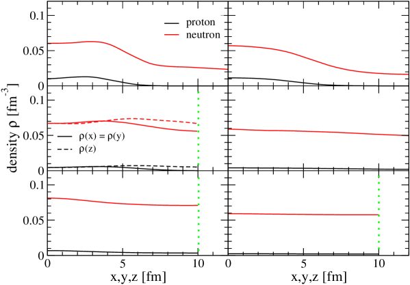
Figure 1: (Color online) Density distributions resulting from density dependent relativistic mean field (DDRMF) calculations for protons (black color) and neutrons (red color) as a function of Cartesian coordinates $x,y,z$. The panels in the left column refer to zero temperature calculations at the densities 0.020 fm^-3 (top), 0.057 fm^-3, and 0.067 fm^-3 (bottom), while those in the right column are obtained for the temperature $T=5$ MeV at the densities 0.018 fm^-3 (top), 0.044 fm^-3, and 0.057 fm^-3.

The top panel in the left column represents a nuclear structure at a baryonic density of 0.020 fm^-3 at zero temperature. In this case the density profiles are identical in all three Cartesian directions. In the center a quasi–nuclear of the WS cell droplet structure is formed with a neutron sea between these quasi–nuclei.

 

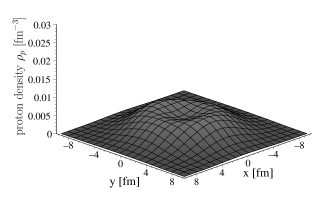
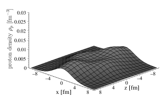
Figure 2: Proton density distribution in the $z=0$ and the $y=0$ plane for the density dependent relativistic mean field (DDRMF) calculation at an average density of $\rho=0.057$ fm${}^{-}3$.

Increasing the baryonic density to $\rho$ = 0.057 fm^-3, we obtain the second panel in the left column of Fig. 1. In this case the proton density shows almost the same value along one axis, which is chosen to be the $z$–direction (dashed curves), while it drops to zero, if the values for $x$ and $y$ tend towards $R$. Here we find a so–called rod or Spaghetti-shape structure for the proton density distribution. Note, however, that the density distribution is not as simple as these names rod-structure or Spaghetti-structure suggest. This can be seen from the complete density-distribution in the $y=0$ (or $x=0$, which is identical for this geometry), as it is displayed in Fig. 2. There is a dip in the center of the quasi-nuclear structure and the density distributions exhibit a structure, which is close to those of nuclei with strong prolate deformations, which are aligned and touch each other along the $z$-axis.

 

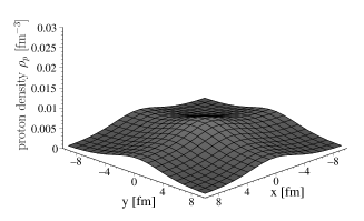
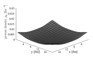
Figure 3: Proton density distribution in the $z=0$ plane for the density dependent relativistic mean field (DDRMF) calculation at an average density of $\rho=0.067$ fm${}^{-}3$. The surface plot on the left shows the density distribution with the origin in the center, while in one on the right hand side the origin is shifted to the corner.

At larger densities the density distributions show again the same distribution along the axis in all Cartesian directions. It is still slightly enhanced in the center and drops only by a small amount from the center to the boundary of the cell. An example of such a structure at the baryon density of 0.067 fm^-3 is displayed in Fig. 1 in the bottom panel of the left column. However, the proton density distribution in the $z=0$ plane displayed on the left in Fig. 3 provides a more detailed picture of the geometric structures at this density: The proton density drops along the diagonals, which implies that the regions of high densities in the center of the WS cells are connected by arms along the Cartesian axes. From this point of view this structure may be called a grid structure. If, however, the coordinates are shifted in such a way, that the centers of the quasi-nuclei are in the corners of the box as it is displayed in Fig. 3 on the right, one finds that this structure can also be interpreted as a bubble structure. Summarizing we observe a grid structure with bubbles in between, which provides a last step of a smooth transition to homogeneous matter.

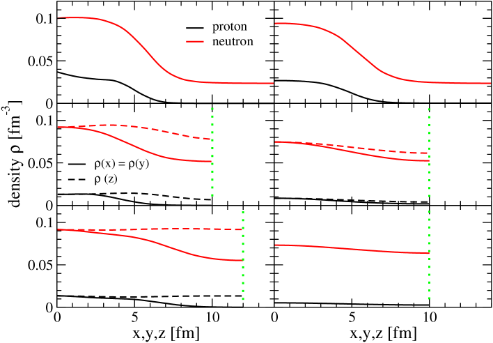
Figure 4: (Color online) Comparison of density distributions at finite temperature with those at zero temperature resulting from Skyrme HF calculations for protons (black color) and neutrons (red color) as a function of Cartesian coordinates $x,y,z$. The panels in the left column refer to $T=0$ MeV calculations at the average densities 0.0271 fm^-3 (top), 0.0565 fm^-3, and 0.0625 fm^-3 (bottom), while those in the right column are obtained for $T=5$ MeV at the baryon densities 0.0273 fm^-3 (top), 0.0545 fm^-3, and 0.0648 fm^-3.

These kind of geometrical structures and others have also been obtained in a recent investigation employing the Skyrme Hartree–Fock approach Goegelein:2007 . Some typical results for the density profiles at zero temperature are presented in the left column of Fig. 4. These examples represent a droplet structure ($\rho$ = 0.027 fm^-3, top panel), a rod-structure with a reduced density at $z=R$ as compared to $z=0$ ($\rho$ = 0.0565 fm^-3, middle panel) and a rod-structure with constant densities along the $z$-axis ($\rho$ = 0.0625 fm^-3, bottom panel)

Comparing the DDRMF results of Fig. 1 with these density distributions obtained from non–relativistic Skyrme calculations, we see that in case of Skyrme Hartree–Fock calculations the different structures are more pronounced. Also we observe a slab structure in the Skyrme Hartree–Fock approach, which is absent in the DDRMF calculations. This differences may originate from the finite range of the NN interaction in the DDRMF approach as compared to the zero-range forces of the Skyrme model.

In both cases we find that the microscopic calculations in a Cartesian WS cell for densities in the range of 0.01 fm^-3 to 0.1 fm^-3 lead to quite a variety of shapes and quasi-nuclear structures with smooth transitions in between, which may be characterized as quasi–nuclei, rod structures, slab structures, which are all embedded in a sea of neutrons and, finally, the homogeneous matter. In the left part of table 4 the densities, at which the transitions from one shape to the other occur at $T=0$, are listed for Skyrme HF calculations as well as for the density dependent relativistic mean field approach.

	Skyrme		DDRMF		Skyrme		DDRMF
	HF	TF	H	TF	HF	TF	H	TF
droplet–rod	0.042	0.066	0.057	0.048	0.040	0.048	0.044	0.045
rod–slab	0.070	0.078	-	-	-	-	-	-
slab–homogeneous	0.080	0.085	0.064	0.061	0.065	0.048	0.044	0.045
	T = 0				T = 5 MeV

Table 4: Comparison of densities at which shape transitions occur using the Skyrme and the density dependent relativistic mean field (DDRMF) approach. Results are compared, employing the microscopic Hartree–Fock (HF), the mean-field or Hartree (H) and the Thomas–Fermi (TF) approximation. Results displayed in the left part of the table refer to a temperature of $T=0$, whereas those listed in the right part were obtained for $T=5$ MeV. All entries are presented in fm^-3.

Performing DDRMF calculations at the finite temperature $T=5$ MeV we obtain for neutrons and protons density distributions as displayed in the right column in Fig. 1. Inspecting these plots, it is clear that the geometrical structures observed for $T=0$ persist to some extent also at finite temperatures as large as $T=5$ MeV. It is also obvious, however, that finite temperature effects tend to dissolve these structures: The structures in the right column at corresponding or even lower densities are less pronounced than those in the left column of Fig. 1. The same features can also be observed for the Skyrme Hartree–Fock approach, as can be seen from Fig. 4.

The transition densities for all calculations in the WS cell at a temperature of $T=5$ MeV are summarized in the right part table 4. If we compare the Skyrme HF transition densities at $T=5$ MeV with the zero temperature results, the transition densities are lower at finite temperature and the slab structure disappears. The results obtained from the DDRMF approach do not any more show a rod structure, but the transition from the droplet structure to homogeneous matter occurs via a grid structure, which can be regarded as transition to the homogeneous phase like in the zero temperature case.

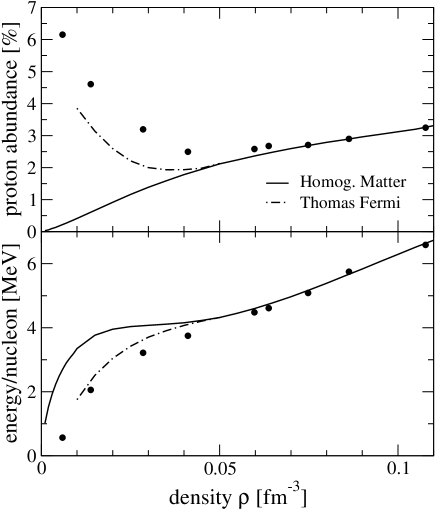
Figure 5: Proton–abundances and energy per nucleon resulting from density dependent relativistic mean-field calculations (DDRMF) at different densities. The results evaluated in cubic Wigner Seitz cells (circles) are compared to those of homogeneous infinite matter (solid lines) and corresponding Thomas–Fermi calculations (dashed lines).

A comparison of the proton abundances and the energy per nucleon obtained within the DDRMF model in a Wigner–Seitz cell for zero temperature are displayed in Fig. 5. The solid lines represents the homogeneous matter results, while the circles display the results obtained from the microscopic density dependent relativistic mean field calculation in the cubic box. At densities larger than about 0.08 fm^-3 the proton abundances and energies coincide for homogeneous matter and the microscopic calculation, which implies that for densities larger than 0.08 fm^-3 the formation of inhomogeneous structures does not provide any gain in energy for baryonic matter in $\beta$-equilibrium. For lower densities, however, the non–homogeneous structures provide a gain in binding energy up to 1.7 MeV per nucleon. These quasi-nuclear structures, embedded in a sea of neutron matter, are also responsible for the enhancement of proton abundances at small global densities: the protons are constrained to the regions of enhanced densities.

One can try to simulate these features resulting from the non–homogeneous structures using the Thomas–Fermi approximation. Like in a Ref. Goegelein:2007 we want to compare the DDRMF results with the Thomas–Fermi calculation based on a local density approximation of the energy density for homogeneous nuclear matter. In our Thomas–Fermi (TF) calculations we use a parameterization for the density distributions like in Oyamatsu:2007

$$\rho_{i}(r)=\begin{cases}(\rho_{i}^{in}-\rho_{i}^{out})\left[1-\left(\frac{r}{R_{i}}\right)^{t_{i}}\right]^{3}+\rho_{i}^{out},&r<R_{i}\\ \rho_{i}^{out},&R_{i}\leq r,\ \ \ \ i=p,n,\end{cases}$$ (43)

where the central density $\rho_{i}^{in}$, the peripheral density $\rho_{i}^{out}$, the structure radius $R_{i}$ and an exponent $t_{i}$ are the variational parameters completed by the box-size $R$ and the proton abundance. As an alternative a Wood–Saxon type density parameterization has been considered, but it turned out that the results are comparable and only the surface energy constant $F_{0}$ has to be readjusted. For the description of rod–shape quasi–nuclear structures cylindrical coordinates are used to parameterize the dependence of the densities on the radial coordinate in a way corresponding to eq.(43). In the case of quasi–nuclear structures in form of slab–shapes these parameterizations are considered for the dependence of the densities on the Cartesian $z$-coordinate.

Assuming those density distributions, the TF energy is calculated as a sum of the bulk energy, i.e. the integrated nuclear–matter energy densities, the Coulomb energy, plus the contribution of a surface term of the form Oyamatsu:2007 ; Oyamatsu:1993

$$E_{\text{surf}}=F_{0}\,\int_{\text{WS-cell}}d^{3}r\,\left|\boldsymbol{\nabla}\rho\right|^{2}\,.$$ (44)

The parameters of the density distribution in(43) are varied to minimize the energy of the system under consideration. The Parameter $F_{0}$ for the surface energy term in (44) has been adjusted in such a way that the TF calculation reproduces the experimental binding energy of the nucleus ${}^{208}Pb$, which has also been reproduced in the DDRMF calculation. This adjustment leads to a value for $F_{0}$ of 61.0 MeV fm⁵, which is rather similar to the value of 68.3 MeV fm⁵, derived in Goegelein:2007 for Skyrme HF case.

Such TF calculations lead to non–homogeneous structures similar to those calculated in DDRMF and we obtain transitions between the various shapes at the densities, which are listed in table 4. Comparing the Thomas–Fermi results to the one obtained from the microscopic DDRMF calculations in Fig. 5 in the density range below 0.05 fm^-3 it is observed that the proton abundance from the Thomas–Fermi calculations are lower and the energy is larger as obtained from the corresponding microscopic DDRMF results. The surface energy constant $F_{0}$ may be readjusted to reproduce the microscopic DDRMF results for the nuclear structures in $\beta$–equilibrium. This leads to a value of $F_{0}$, which is only about half the value for $F_{0}$ derived from the fit to the properties of ²⁰⁸Pb. This suggests to consider a surface constant $F_{0}$, which depends on the isospin asymmetry of the system. This feature is very similar to the one observed applying the Skyrme Hartree–Fock approachGoegelein:2007 .

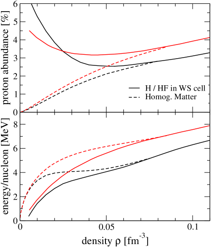
Figure 6: (Color online) Comparison of proton abundances and energy per nucleon obtained from DDRMF (black color) and Skyrme Hartree–Fock calculations (red color). Solid lines are obtained from a polynomial fit to the DDRMF or the Skyrme Hartree–Fock calculation in the cubic Wigner–Seitz cell, while dashed lines represent the results for homogeneous infinite nuclear matter.

To enable further explorations on the differences between the predictions for the “pasta-phase” derived from DDRMF and Skyrme HF calculations, results of those two approaches for the energy per nucleon and the proton abundances are directly compared in Fig 6 The results of both models show a similar overall behavior and both predict a transition to the homogeneous phase at a density of about 0.08 fm^-3. Looking into details, however, one finds rather interesting differences: The energy per nucleon is larger for the Skyrme calculation at all densities considered in Fig 6. This is in line with the fact that the Skyrme force SLy4, which we have used here, yields a parameter for the symmetry energy $a_{S}$ of 32 MeVchabanat , which is larger than the one derived from DDRMF (see table 2). Note, however, that the symmetry energy coefficient is determined at saturation density, whereas here we are comparing structures at half the saturation density and below. A larger symmetry energy at those small density would also explain the larger proton abundances obtained in the Skyrme approach.

The energy gain due to the formation of non–homogeneous structures is slightly larger for the Skyrme approach at medium densities of 0.02 to 0.08 fm^-3. This is in line with our observation made in the discussion above, that the geometrical structures determined in Skyrme HF are typically more pronounced than those extracted from DDRMF. At very small densities the DDRMF leads to a larger gain in energy forming non–homogeneous matter distributions. At these densities the DDRMF calculations in the WS cell also predict a larger proton abundance than the Skyrme approach.

The parameters of the Skyrme interaction have only been adjusted to the data of finite nuclei and the saturation point of symmetric matter, i.e. data of nuclear systems at normal densities and proton-neutron asymmetries. The parameterization of the DDRMF on the other side also reproduces those data but is furthermore based on a realistic NN interaction. Therefore, we trust in the predictions of the DDRMF approach for this region of small densities and large proton-neutron abundances more than in those based on the Skyrme Hamiltonian.

Finally, we are going to discuss the effects of finite temperature. For that purpose Fig. 7 displays results for proton abundances and the energy per nucleon evaluated in the DDRMF approach at a temperature of $T=5$ MeV. The lower panel in Fig. 7 shows two curves: the energy per nucleon (upper curve) and the free energy per nucleon (lower curve). Comparing with the results obtained from zero temperature DDRMF calculations we recognize that the results for $T=5$ show a minimum for the energy per nucleon at a density of about 0.05 fm^-3, while the zero temperature results show no minimum. However, the free energy, which is the energy of consideration, is lower than the energy in the $T=0$ case and rises with a larger slope, which means that the finite temperature increases the pressure derived from the free energy.

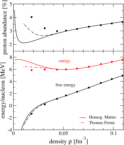
Figure 7: Proton abundances and energy per nucleon resulting from density dependent relativistic mean field calculations at the temperature $T=5$ MeV. The results evaluated in cubic Wigner–Seitz cells (circles) are compared to those of homogeneous infinite matter (solid lines).

The energies resulting from the DDRMF calculations, which allow for non–homogeneous structure yield a gain in energy for densities below 0.05 fm^-3. This means that a temperature of 5 MeV lowers the critical density for the formation of local structures from 0.08 fm^-3 at $T=0$ to 0.05 fm^-3 at $T=5$ MeV. At values below this critical density, the gain in the free energy at finite temperature turns out to be considerably smaller than in the zero temperature limit. This reflects the feature that finite temperature effects tend to suppress the formation of density fluctuations. Note, that these small differences between the free energy of the homogeneous and inhomogeneous structures is to quite some extent due to the enhancement of the entropy in the inhomogeneous case. We observe the same features in Skyrme HF calculations at finite temperature. Finite temperature also reduces the variety of geometrical shapes in the Skyrme HF as well as in the DDRMF approach (see table 4).

Fig. 7 also displays results from Thomas-Fermi calculations. In this case the temperature dependence is contained only in the the bulk contribution, i.e. the integrated nuclear–matter energy densities calculated at the finite temperature. The parameter for the surface energy $F_{0}$ is still adjusted to reproduce the properties of ²⁰⁸Pb at $T=0$. As discussed above one could now try to fit this constant $F_{0}$ in such a way that we reproduce results for the energy, the free energy and proton abundances of the DDRMF approach. This readjustment leads to a value of 27 MeV fm⁵ for the parameterization of eq.(43). The value is lower by about 15% compared to the corresponding one at zero temperature. Hence a slight reduction of the surface energy constant $F_{0}$ could improve the Thomas–Fermi approach at finite temperature.

V Conclusion

Density dependent relativistic mean field (DDRMF) calculations have been performed to study the structure of baryonic matter in $\beta$-equilibrium with electrons in a region of densities between 0.01 and 0.1 nucleons fm^-3. A parameterization of the density dependent meson-nucleon coupling constants has been developed, which is based on microscopic Dirac Brueckner Hartree Fock (DBHF) calculations and reproduces the saturation point of nuclear matter as well as the bulk properties of finite nuclei. Since this parameterization yields a good description of normal nuclei, i.e. baryonic matter at normal density and small proton - neutron asymmetries but is also based on a realistic interaction which describes the scattering of two nucleons in the vacuum, it should give more reliable results for the baryonic structure at small densities and large proton-neutron asymmetries than corresponding calculations, which are based on purely phenomenological Hamiltonians like the Skyrme forces. The parameterization of the coupling constants in terms of analytic functions makes it easily accessible.

The DDRMF calculations are performed for zero temperature as well as finite temperature in a periodic lattice of Wigner-Seitz (WS) cells of cubic shape. Pairing correlations are taken into account within the framework of the finite temperature BCS approximation assuming a density-dependent pairing force of zero range.

At densities below 0.08 nucleons fm^-3 the DDRMF approach predicts non-homogeneous structures, which are similar to those predicted by Thomas-Fermi or Skyrme Hartree-Fock calculations for the “pasta-phase” of matter in the crust of neutron stars. The structures obtained in the DDRMF calculations, however, are typically less pronounced than the corresponding structures resulting from Skyrme Hartree–Fock calculations. This may be a consequence of the finite range of the interaction in DDRMF as compared to the zero-range Skyrme forces. Also it turns out that the gain in energy due to the formation of non–homogeneous density distributions is slightly smaller in the DDRMF as compared to Skyrme HF. Also the DDRMF yields a smaller symmetry energy at the low densities, which provides smaller proton abundances.

The effects of finite temperature tend to reduce the disposition of the baryonic matter to form non–homogeneous structures. This is driven by the larger entropy of the non–homogeneous matter as compared to the homogeneous phase. This leads to a reduction of the critical density for the formation of non–homogeneous structures. It drops from 0.08 nucleons fm^-3 at $T=0$ to 0.05 nucleons fm^-3 at $T=5$ MeV. At densities below the critical densities, the gain in the free energy of the non–homogeneous as compared to the homogeneous realization is smaller and the resulting geometrical structures are less pronounced in the case of finite temperature.

An attempt has been made to reproduce the results of the microscopic Skyrme HF and DDRMF calculation by means of the Thomas-Fermi (TF) approximation. Main features like the critical densities for the formation of geometrical structures of various shapes, the energies and the proton abundances can be reproduced, if one considers a parameter for the surface term, which is reduced with increasing proton asymmetry and with temperature.

This work has been supported by the European Graduate School “Hadrons in Vacuum in Nuclei and Stars” (Basel, Graz, Tübingen), which obtains financial support by the DFG and received support from the GSI project TUEMUE and by the Spanish Ministry of Education and Science under grant no. SB-2005-0131.

References

- (1) M. Baldo, Nuclear Methods and the Nuclear Equation of State, Int. Rev. of Nucl. Phys, Vol. 9 (World Scientific, Singapore, 1999).
- (2) H. Müther and A. Polls, Prog. Part. Nucl. Phys. 45, 243 (2000).
- (3) S.C. Pieper, K. Varga, and R.B. Wiringa, Phys. Rev. C 66, 044310 (2002).
- (4) M.R. Anastasio, L.S. Celenza, W.S. Pong, and C.M. Shakin, Phys. Rep. 100, 327 (1983).
- (5) R. Brockmann and R. Machleidt, Phys. Rev. C 42, 1965 (1990).
- (6) B. Ter Haar and R. Malfliet, Phys. Rep. 149, 207 (1987).
- (7) H. Huber, F. Weber, and M.K. Weigel, Phys. Lett. B 317, 485 (1993).
- (8) B.D. Serot and J.D. Walecka, Adv. Nucl. Phys. 16, 1 (1986).
- (9) O. Plohl and C. Fuchs, Phys. Rev. C 74, 034325 (2006).
- (10) Z. H. Li, U. Lombardo, H. J. Schulze, W. Zuo, L. W. Chen and H. R. Ma, Phys. Rev. C 74, 047304 (2006).
- (11) T.H.R. Skyrme, Nucl. Phys. 9, 615 (1959).
- (12) D. Vautherin and D.M. Brink, Phys. Rev. C5, 626, (1972).
- (13) P. Bonche and D. Vautherin, Nucl Phys. A372, 496 (1981).
- (14) F. Montani, C. May, and H. Müther, Phys. Rev. C 69, 065801 (2004).
- (15) P. Gögelein and H. Müther, Phys. Rev. (2007) in print.
- (16) E. Schiller and H. Müther, Eur. Phys. J. A11, 15 (2001).
- (17) F. Hofmann, C.M. Keil, and H. Lenske, Phys. Rev. C 64, 034314 (2001).
- (18) E.N.E. van Dalen, C. Fuchs, and A. Faessler, Eur. Phys. J. A 31, 29 (2007).
- (19) T. Klähn, D. Blaschke, S. Typel, E.N.E. van Dalen, A. Faessler, C. Fuchs, T. Gaitanos, H. Grigorian, A. Ho, E.E. Kolomeitsev, M. C. Miller, G. Röpke, J. Trümper,D. N. Voskresensky, F. Weber, and H. H. Wolter, Phys. Rev. C 74, 035802 (2006).
- (20) J.D. Bjorken and S.D. Drell, Relativistic Quantum Mechanics, McGraw-Hill, New York, 1964.
- (21) C. Fuchs, H. Lenske, and H.H. Wolter, Phys. Rev. C 52, 3043 (1995).
- (22) R. Fritz and H. Müther, Phys. Rev. C 49, 633 (1994);R. Fritz, Ph-D thesis, Tübingen (1994).
- (23) A.L. Goodman, Nucl. Phys. A352, 30 (1981).
- (24) H. Shen, H. Toki, K. Oyamatsu, K. Sumiyoshi, Nucl. Phys. A637, 435 (1998).
- (25) H. Shen, H. Toki, K. Oyamatsu, K. Sumiyoshi, Prog. Theor. Phys. 100, 1013 (1998).
- (26) F. de Jong and H. Lenske, Phys. Rev. C 58, 890 (1998).
- (27) E.N.E. van Dalen, C. Fuchs, and A. Faessler, Nucl. Phys. A744, 227 (2004).
- (28) T. Gross-Boelting, C. Fuchs, and Amand Faessler, Nucl. Phys. A648, 105 (1999).
- (29) P. Ring, Prog. Part. Nucl. Phys. 37, (1996) 193.
- (30) C. Sturm et al. [KaoS Coll.], Phys. Rev. Lett. 86, 39 (2001); C. Fuchs, A. Faessler, E. Zabrodin, and Y.M. Zheng, Phys. Rev. Lett. 86, 1974 (2001); C. Fuchs, Prog. Part. Nucl. Phys. 56, 1 (2006).
- (31) D. T. Khoa, W. von Oertzen, H. G. Bohlen and S. Ohkubo, J. Phys. G 33, R111 (2007); D. T. Khoa et al., Nucl. Phys. A 759, 3 (2005)
- (32) K. Oyamatsu and K. Iida, Phys. Rev. C75, 015801 (2007).
- (33) K. Oyamatsu, Nucl. Phys. A561, 431 (1993).
- (34) E. Chabanat, P. Bonche, P. Haensel, J. Meyer, and R. Schaeffer, Nucl. Phys. A 635, 231 (1998).