Lattice study of monopoles in the Electroweak theory

Abstract:

We investigated numerically properties of Nambu monopoles in lattice Electroweak theory at realistic values of $\alpha$ and $\theta_{W}$. Our choice of parameters of lattice Lagrangian corresponds to large values of the Higgs boson mass $M_{H}>2M_{W}$. We find that the density of Nambu monopoles cannot be predicted by the choice of the initial parameters of Electroweak theory and should be considered as the new external parameter of the theory. We also investigate the difference between the versions of Electroweak theory with the gauge groups $SU(2)\otimes U(1)$ and $SU(2)\otimes U(1)/Z_{2}$. We do not detect any difference at $\alpha\sim\frac{1}{128}$. However, such a difference appears in the strong coupling region and is related to the properties of monopoles constructed of the hypercharge field.

1 Introduction

The qualitative lattice investigation of the properties of Nambu monopoles[1] in the Standard Model has been performed both at zero and finite temperatures in the unphysical region of large coupling constants in [2]. Nambu monopoles are found to be condensed in the symmetric phase of lattice theory (and above the Electroweak transition in the finite temperature theory). Here we continue this investigation for realistic values of the renormalized coupling constants ($\alpha\sim 1/128$ and $\theta_{W}=\pi/6$) within the zero temperature theory.

Earlier we considered the appearance of an additional discrete symmetry in the fermion sector of the Standard Model[2, 3, 4]. This additional symmetry allows to define Standard Model with the gauge group $SU(3)\times SU(2)\times U(1)/{\cal Z}$, where ${\cal Z}$ is equal to $Z_{6}$, or to one of its subgroups: $Z_{3}$ or $Z_{2}$. The emergence of $Z_{6}$ symmetry in technicolor models was considered in [5].

Here we use two lattice realizations of the Electroweak theory: with the gauge groups $SU(2)\times U(1)/Z_{2}$, and $SU(2)\times U(1)$, respectively.

2 Lattice models under investigation

We consider lattice Weinberg - Salam Model in quenched approximation. The model contains the gauge field ${\cal U}=(U,\theta)$, where $\quad U\in SU(2),\quad e^{i\theta}\in U(1)$ are realized as link variables. The potential for the scalar field is considered in its simplest form [2] in the London limit, i.e., in the limit of infinite bare Higgs mass. From the very beginning we fix the unitary gauge.

For the case of $SU(2)\times U(1)/Z_{2}$ symmetric model we chose the action of the form

$$S_{g} = \beta\!\!\sum_{\rm plaquettes}\!\!((1-\mbox{${\small\frac{1}{2}}$}\,{\rm Tr}\,U_{p}\cos\theta_{p})+\mbox{${\small\frac{1}{2}}$}(1-\cos 2\theta_{p}))+$$ (1)

$$+\gamma\sum_{xy}(1-Re(U^{11}_{xy}e^{i\theta_{xy}})),$$

where the plaquette variables are defined as $U_{p}=U_{xy}U_{yz}U_{wz}^{*}U_{xw}^{*}$, and $\theta_{p}=\theta_{xy}+\theta_{yz}-\theta_{wz}-\theta_{xw}$ for the plaquette composed of the vertices $x,y,z,w$.

For the case of the conventional $SU(2)\times U(1)$ symmetric model we use the action

$$S_{g} = \beta\!\!\sum_{\rm plaquettes}\!\!((1-\mbox{${\small\frac{1}{2}}$}\,{\rm Tr}\,U_{p})+3(1-\cos\theta_{p}))+$$ (2)

$$+\gamma\sum_{xy}(1-Re(U^{11}_{xy}e^{i\theta_{xy}})).$$

In both cases the bare Weinberg angle is $\theta_{W}=\pi/6$, which is close to its experimental value. The renormalized Weinberg angle is to be calculated through the ratio of the lattice masses: ${\rm cos}\,\theta_{W}=M_{W}/M_{Z}$. The bare electromagnetic coupling constant $\alpha$ is expressed through $\beta$ as $\alpha=1/4\pi\beta$. However, the renormalized coupling extracted from the potential for infinitely heavy fermions differs from this simple expression, as will be shown in the next sections.

3 The results

3.1 Phase diagram

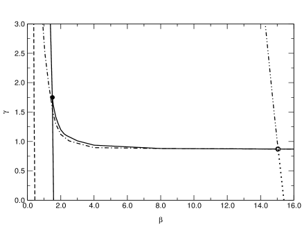
Figure 1: The phase diagrams of the models in the $(\beta,\gamma)$-plane.

The phase diagrams of the two models under consideration are presented in figure $1$. The dashed vertical line represents the phase transition in the $SU(2)\otimes U(1)$-symmetric model. This is the confinement-deconfinement phase transition corresponding to the $U(1)$ constituents of the model. The same transition for the $SU(2)\otimes U(1)/Z_{2}$-symmetric model is represented by the solid vertical line. The dashed horizontal line corresponds to the transition between the broken and symmetric phases of model A. The continuous horizontal line represents the same transition in model B. Interestingly, in the $SU(2)\otimes U(1)/Z_{2}$ model both transition lines meet, forming a triple point. Much attention was paid to this fact in [2].

Real physics is commonly believed to be achieved within the phases of the two models situated in the right upper corner of Fig. $1$. The double-dotted-dashed vertical line on the right-hand side of the diagram represents the line, where the renormalized $\alpha$ is constant and equal to $1/128$.

All simulations were performed on lattices of sizes $8^{4}$ and $16^{4}$. Several points were checked using a lattice $24^{4}$. In general we found no significant difference between the mentioned lattice sizes.

3.2 The masses

The following variables are considered as creating a $Z$ boson and a $W$ boson, respectively: $Z_{xy}=Z^{\mu}_{x}\;={\rm sin}\,[{\rm Arg}U_{xy}^{11}+\theta_{xy}]$, $W_{xy}=W^{\mu}_{x}\,=\,U_{xy}^{12}e^{i\theta_{xy}}$. In order to evaluate the masses of the $Z$-boson and Higgs boson we use the zero - momentum correlators: $\sum_{\bar{x},\bar{y}}\langle\sum_{\mu}Z^{\mu}_{x}Z^{\mu}_{y}\rangle\sim e^{-M_{Z}|x_{0}-y_{0}|}+e^{-M_{Z}(L-|x_{0}-y_{0}|)}$, $\sum_{\bar{x},\bar{y}}\langle H_{x}H_{y}\rangle\sim e^{-M_{H}|x_{0}-y_{0}|}+e^{-M_{H}(L-|x_{0}-y_{0}|)}+const$. In lattice calculations we used three different operators that create Higgs bosons: $H_{x}=\sum_{y}|W_{xy}|^{2}$, $H_{x}=\sum_{y}Z^{2}_{xy}$, and $H_{x}=\sum_{y}Re(U^{11}_{xy}e^{i\theta_{xy}})$. In all cases $H_{x}$ is defined at the site $x$, the sum $\sum_{y}$ is over its neighboring sites $y$.

After fixing the unitary gauge, lattice Electroweak theory becomes a lattice $U(1)$ gauge theory. The $U(1)$ gauge field is $A_{xy}=A^{\mu}_{x}\;=\,[-{\rm Arg}U_{xy}^{11}+\theta_{xy}]\,{\rm mod}\,2\pi$. The usual Electromagnetic field is $A_{\rm EM}=A+Z^{\prime}-2\,{\rm sin}^{2}\,\theta_{W}Z^{\prime}$, where $Z^{\prime}=[{\rm Arg}U_{xy}^{11}+\theta_{xy}]{\rm mod}2\pi$.

The $W$ boson field is charged with respect to the $U(1)$ symmetry. Therefore we fix the lattice Landau gauge in order to investigate the $W$ boson propagator. The lattice Landau gauge is fixed via minimizing (with respect to the $U(1)$ gauge transformations) of the following functional: $F=\sum_{xy}(1-\cos(A_{xy})).$ Then we extract the mass of the $W$ boson from the correlator $\sum_{\bar{x},\bar{y}}\langle\sum_{\mu}W^{\mu}_{x}(W^{\mu}_{y})^{\dagger}\rangle\sim e^{-M_{W}|x_{0}-y_{0}|}+e^{-M_{W}(L-|x_{0}-y_{0}|)}$ The renormalized Weinberg angle is to be calculated through the ratio of the lattice masses: ${\rm cos}\,\theta_{W}=M_{W}/M_{Z}$.

In the region $\beta\in(10,20)$, $\gamma\in(1,2)$ we found no difference between the two versions of lattice Electroweak theory. Therefore, we omit mentioning to what particular model the considered quantity belongs in this region of coupling constants.

$W$-boson and $Z$-boson masses are found to change very slowly with the variation of $\beta$. The dependence on $\gamma$ seems to be stronger. Both gauge boson masses grow with the decrease of $\gamma$. We evaluate both masses of $W$- and $Z$-bosons to be $0.23\pm 0.02$ at $\gamma=1,\beta=15$. We cannot calculate the renormalized Weinberg angle at this point with reasonable accuracy.

Unfortunately, the statistical errors do not allow us to calculate the Higgs boson mass with a reasonable accuracy. Our data only allow us to draw the conclusion that $M_{H}$ is larger than $2M_{W}$.

3.3 The renormalized coupling

The bare constant $\alpha=e^{2}/4\pi$ (where $e$ is the electric charge) can be easily calculated in our lattice model. It is found to be equal to $1/(4\pi\beta)$. Therefore, its physical value $\alpha(M_{Z})\sim 1/128$ could be achieved at values of $\beta$ in some vicinity of $10$. This naive guess is, however, to be corrected by the calculation of the renormalized coupling constant $\alpha_{R}$. We perform this calculation using the potential for infinitely heavy external fermions. We consider Wilson loops for the right-handed external leptons: ${\cal W}^{\rm R}_{\rm lept}(l)=\langle{\rm Re}\,\Pi_{(xy)\in l}e^{2i\theta_{xy}}\rangle.$ Here $l$ denotes a closed contour on the lattice. We consider the following quantity constructed from the rectangular Wilson loop of size $r\times t$: ${\cal V}(r)=\lim_{t\rightarrow\infty}\frac{{\cal W}(r\times t)}{{\cal W}(r\times(t+1))}.$ At large enough distances we expect the appearance of the Coulomb interaction ${\cal V}(r)=-\frac{\alpha_{R}}{r}+const.$

The renormalized coupling constant $\alpha$ is found to be close to the realistic value $\alpha(M_{Z})=1/128$ along the line represented in Fig. $1$. Actually, a linear dependence of the potential for infinitely heavy right-handed leptons on $1/r$ is observed already for $r=1$. Therefore we treat this constant as $\alpha_{R}(1/a)=\alpha_{R}(100{\rm GeV})\sim\alpha_{R}(M_{Z})$.

3.4 Nambu monopole density and percolation probability

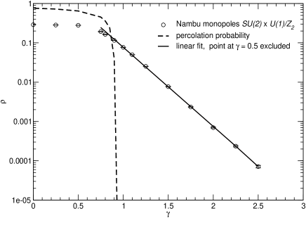
Figure 2: Nambu monopole density and percolation probability as a function of $\gamma$ along the line of constant $1/\alpha_{R}=128$.

According to [6] the worldlines of the quantum Nambu monopoles could be extracted from the field configurations as follows:

$$j_{Z}=\delta\Sigma=\frac{1}{2\pi}{}^{*}d([dZ^{\prime}]{\rm mod}2\pi)$$ (3)

(The notations of differential forms on the lattice [7] are used here.) The monopole density is defined as $\rho=\left\langle\frac{\sum_{\rm links}|j_{\rm link}|}{4L^{4}}\right\rangle,$ where $L$ is the lattice size.

In order to investigate the condensation of monopoles we use the percolation probability $\Pi(A)$. It is the probability that two infinitely distant points are connected by a monopole cluster (for more details of the definition see, for example, [8]). In Fig. $5$ we show Nambu monopole density and percolation probability as a function of $\gamma$ along the line of constant renormalized $\alpha_{R}=1/128$. It is clear from Fig. $5$ that the percolation probability is the order parameter of the transition from the symmetric to the broken phase. In order to compare the position of the transition between the symmetric and broken phases with the point where percolation probability vanishes, we investigate the susceptibility $\chi=\langle H^{2}\rangle-\langle H\rangle^{2}$ extracted both from $H_{Z}=\sum_{y}Z^{2}_{xy}$ and $H_{W}=\sum_{y}|W|^{2}_{xy}$ .

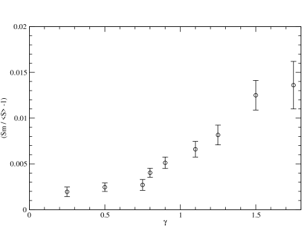
Figure 3: Plaquette action near monopole trajectories along the line of constant $1/\alpha_{R}=128$.

The monopole worldline lives on the dual lattice. Each point of the worldline is surrounded by a three - dimensional hypercube of the original lattice. We measure the plaquette part of the action $S^{\rm mon}_{p}$ on the plaquettes that belong to those $3$-dimensional hypercubes (normalized by the number of such plaquettes). The excess of the plaquette action near monopole worldlines over the mean plaquette part of the action $S_{p}$ is denoted by $\Delta S_{p}=\frac{1}{S_{p}}(S^{\rm mon}_{p}-S_{p}).$ Very roughly $\Delta S_{p}$ can be considered as measuring the magnetic energy (both $SU(2)$ and $U(1)$), which is carried by Nambu monopoles.

We also measure $S^{\rm mon}_{l}$, which is the part of the action $S^{\rm mon}_{l}$ on the links of the original lattice that connect vertices of the two incident $3$-dimensional hypercubes mentioned above. The excess of this link action near monopole worldlines over the mean link part of the action $S_{l}$ is denoted by $\Delta S_{l}=\frac{1}{S_{l}}(S^{\rm mon}_{l}-S_{l}).$ For the simplicity of the calculations we get only one of the $8$ links that connect incident hypercubes. The magnetic energy $\Delta S_{p}$ carried by Nambu monopole is presented in Fig. $7$. The behavior of both $\Delta S_{p}$ and $\Delta S_{l}$ shows that a quantum Nambu monopole may indeed be considered as a physical object.

3.5 Evaluation of the lattice spacing

The physical scale is given in our lattice theory by the value of the $W$-boson mass $M^{phys}_{W}\sim 80$ GeV. Therefore the lattice spacing is evaluated to be $a\sim[80{\rm GeV}]^{-1}M_{W}$, where $M_{W}$ is the $W$ boson mass in lattice units.

The real continuum physics should be approached along the the line of constant $\alpha_{R}=\frac{1}{128}$, i.e. along the line of constant physics (at this point we omit consideration of $\theta_{W}$ as according to our estimates it does not vary crucially along this line). We investigated the dependence of the ultraviolet cutoff $\Lambda=a^{-1}=(80~{}{\rm GeV})/M_{W}$ on $\gamma$ along the line of constant physics. It occurs that $\Lambda$ is increasing slowly along this line with decreasing $\gamma$ and achieves the value $350\pm 30$ GeV at the transition point between the physical Higgs phase and the symmetric phase. According to our results this value does not depend on the lattice size. This means that the largest achievable value of the ultraviolet cutoff is equal to $350\pm 30$ GeV if the potential for the Higgs field is considered in the London limit.

Our lattice study also demonstrates another peculiar feature of Electroweak theory. If we are moving along the line of constant $\alpha=1/128$, then the Nambu-monopole density decreases with increasing $\gamma$ (for $\gamma>1$). Its behavior is approximated with a nice accuracy by the simple formula: $\rho\sim e^{2.08-4.6\gamma}.$

Naively one may think that the density should decrease with increasing ultraviolet cutoff. However, it occurs that the situation is inverse. This means that the density of Nambu-monopoles is not fixed by the initial values of the coupling constants and should be considered as an additional parameter of Electroweak theory.

4 Conclusions

We investigated lattice Electroweak theory numerically at realistic values of the coupling constants and for Higgs mass larger than $2M_{W}$. We found that the two definitions of the theory (with the gauge groups $SU(2)\otimes U(1)/Z_{2}$ and $SU(2)\otimes U(1)$, rescpectively) do not lead to different predictions at these values of the couplings.

Our investigation of the line of constant physics for the infinite bare self coupling of the Higgs field allows us to draw the conclusion that the values of lattice spacings smaller than $(350\pm 30{\rm GeV})^{-1}$ cannot be achieved in principle for this choice of the potential for the Higgs field.

The action density near the Nambu monopole worldlines is found to exceed the density averaged over the lattice in the physical region of the phase diagram. This shows that Nambu monopoles can indeed be considered as physical objects. Their percolation probability is found to be an order parameter for the transition between the symmetric and broken phases. According to our numerical data the density of Nambu monopoles in the continuum theory cannot be predicted by the choice of the usual parameters of the Electroweak theory and should be considered as a new external parameter of the theory.