Spatial image of reaction area from scattering. I:
$SO_{\mu}(2.1)$ algebra formalism.

Abstract

We develop general formalism of how to relate scattering amplitudes for exclusive processes to spatial image of target hadron. More precisely we show how to determine the spatial distribution of outgoing particles in the space of so-called nearest approach parameter. This parameter characterizes the position in the coordinate space the place where the final particle is produced.

I Introduction

Famous experiment by Hofstadter et al. hofstadter demonstrated that hadrons are not point-like particles and they have non-trivial spatial structure. Recently interest to the spatial images of hadrons was revived with development of the theory of hard exclusive processes, which can be systematically studied using formalism of Generalized Parton Distributions (GPDs) (for reviews see reviewGPDs ). It was demonstrated Budkard that GPDs provide an information about spatial distribution of partons in the transverse plane.

In the present paper we develop general formalism of how to relate scattering amplitudes for exclusive processes to spatial image of target hadron. More precisely we show how to determine the spatial distribution of outgoing particles in the space of so-called nearest approach parameter. This parameter characterizes the position in the coordinate space the place where the final particle is produced.

One-particle states of a free relativistic particle are defined by the 10-parametric group of motion of Minkowski space, which is given by generators of the Poincare group: $M_{\mu\nu}$ and $P_{\nu}$. States can be specified by choosing one or another subgroup. It was found that for description of deep inelastic processes it is useful to consider the "infinite momentum frame" Soper1 ; Soper2 . We remind briefly necessary for this paper ingredients.

The three following generators of the Poincare group:

$$B_{1}=\frac{1}{\sqrt{2}}(K_{1}+J_{2})~{},~{}B_{2}=\frac{1}{\sqrt{2}}(K_{2}-J_{1})~{},~{}J_{3}~{},$$ (1)

with

$$K_{i}=M_{i0}~{}~{},~{}~{}\epsilon_{ijk}J_{k}=M_{ij}~{},$$

satisfy the system of commutation relations:

$$\begin{split}&[B_{1},B_{2}]=0~{},\\ &[J_{3},B_{1}]=iB_{2}~{},\\ &[J_{3},B_{2}]=-iB_{1}~{},\\ &[B^{2}_{1}+B^{2}_{2},J_{3}]=0~{},\\ &[p_{i},B_{j}]=i\delta_{ij}p^{+}~{},\\ &[p^{+},B_{i}]=[p^{+},J_{3}]=0~{}.\end{split}$$ (2)

Here $p_{i}$ is the operator of 3-momentum, $p^{+}=\frac{1}{\sqrt{2}}(p_{0}+p_{3})$. The above commutation relations imply that generators $B_{1}$, $B_{2}$ and $J_{3}$ form the $E(2)$ algebra. Casimir operator of this algebra is $B^{2}=B^{2}_{1}+B^{2}_{2}$ . Because of the last commutation relation, this algebra can be realized in the three-dimension momentum space restricted by the condition $p^{+}=const$ on states $|\vec{\lambda},p^{+}\rangle$. These states satisfy equations:

$$\begin{split}&B^{2}|\vec{\lambda},p^{+}\rangle=\lambda^{2}|\vec{\lambda},p^{+}\rangle~{},\\ &B_{1}|\vec{\lambda},p^{+}\rangle=\lambda_{1}|\vec{\lambda},p^{+}\rangle~{},\\ &B_{2}|\vec{\lambda},p^{+}\rangle=\lambda_{2}|\vec{\lambda},p^{+}\rangle~{},\\ &\lambda^{2}=\lambda_{1}^{2}+\lambda_{2}^{2}~{}.\end{split}$$ (3)

Operators $B_{1}$  , $B_{2}\$, $B^{2}$  on the $p^{+}=const$ surface have complicated expression. However in the limiting case of $p_{\bot}/p\ll 1$ the corresponding operators are given by simple expression:

$$B_{1}=-ip^{+}\frac{\partial}{\partial p_{1}}~{},~{}B_{2}=-ip^{+}\frac{\partial}{\partial p_{2}}~{}.$$ (4)

Substituting these operators into equations (3), we obtain the following expression for the corresponding wave function in momentum representation:

$$\langle\vec{p}_{\bot},p^{+}|\vec{\lambda},p^{+}\rangle=\exp\left(i\frac{\vec{p}_{\bot}\cdot\vec{\lambda}}{p^{+}}\right)~{}.$$ (5)

Now if we introduce dimensional parameter

$$\vec{b}=\frac{\vec{\lambda}}{p^{+}}~{},$$

than the wave function (5) has the form of the eikonal kernel in the plane of impact parameter $\vec{b}$. It allows us to interpret in the infinite momentum frame the eigenstates of the algebra (2) $|\vec{\lambda},p^{+}\rangle$, as the states with fixed spatial position in the transverse plane Andrianov ; Huszar . In the infinite momentum frame the transformation from the transverse momentum to the transverse position representation is reduced to simple two-dimensional Fourier transformation (see eq. (5)). That is the transformation which relates the GPDs to the parton distributions in the spatial transverse plane Budkard . Note that such interpretation is possible only in the infinite momentum space, in order to ensure the condition $p_{\perp}/p\ll 1$. For the hard exclusive processes the latter condition corresponds to the condition $t/Q^{2}\ll 1$, here $t$ is the 4-momentum transfer squared and $Q^{2}$ is the hard scale for the process. First, in experiments the ratio $t/Q^{2}$ can be not be not very small and corrections to the eikonal picture can be sizeable. Secondly, the simple two-dimensional Fourier transform can not be used to obtain spatial distributions of partons for hard processes with large transverse momentum transfer (like hadron form factors, wide angle Compton scattering, etc. wide ) Therefore our aim here is to develop general formalism which would allow "spatial imaging" of hadrons in arbitrary reference frame.

We consider another subalgebra of Poincare group. This is subalgebra of operators:

$$d_{i}=\frac{1}{p^{2}}M_{ij}p_{j}~{}.$$ (6)

It is realized on the surface $p^{2}=const$ . Below we analyze in detail this algebra and use it for description and building one particle states with defined quantum numbers.

II Operator of the nearest approach

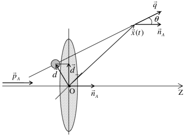
Figure 1: A classical trajectory $\vec{X}(t)$ of an asymptotically free particle with momentum $\vec{q}$ is proceeded into reaction area, is characterized by a vector of maximal approach $\vec{d}$ to the select point "O". In the labor frame this point is a center of target, in the center mass frame it is a meeting point of beams.

Let us consider a trajectory of a free spinless particle, which moves with arbitrary initial conditions (Fig.1) Vall1 :

$$X_{i}(t)=\frac{q_{i}}{\sqrt{\vec{q}^{2}+m^{2}}}(t-t_{0})+\xi_{i}~{},~{}i=1,2,3~{},$$ (7)

with $\vec{q}$ - momentum of the particle , $m$ - mass of the particle. A distance between the particle and the coordinate origin "O"  is

$$D(t)=(\vec{X}(t)\vec{X}(t))^{\frac{1}{2}}~{}.$$

At some moment of time $t=\tau$ the distance $D(\tau)$ has a minimal value. The time $\tau$ is defined by the extremum condition:

$$\frac{d}{dt}D(t)\Big{|}_{t=\tau}=\frac{1}{D(t)}\Big{(}X_{i}(t)\frac{d}{dt}X_{i}(t)\Big{)}\Big{|}_{t=\tau}=0~{}.$$ (8)

Using (7) , we obtain:

$$\begin{split}\tau&=t_{0}-\frac{(\vec{u}\vec{\xi})}{u^{2}}~{},\\ u_{i}&=\frac{q_{i}}{\sqrt{\vec{q}^{2}+m^{2}}}~{}.\end{split}$$ (9)

Substituting $t=\tau$ into $D(t)$, we get the following expression for components of the vector of the nearest approach $d_{i}$:

$$d_{i}=X_{i}(\tau)=-\frac{u_{i}}{u^{2}}(\vec{u}\vec{\xi})+\xi_{i}~{}.$$ (10)

Let us introduce the operator of orbital momentum $L_{k}\ ,\ k=1,2,3$, in usual way:

$$L_{k}=\varepsilon_{klm}\xi_{l}q_{m}~{}.$$ (11)

Then the expression (10) can be rewritten as:

$$d_{i}=\frac{1}{q^{2}}\varepsilon_{ijk}q_{j}L_{k}=\frac{1}{q^{2}}M_{ij}q_{j}~{}.$$ (12)

We see that for each classical trajectory $\vec{X}(t)$ of an asymptotically free particle, which moves out from the reaction area with momentum $\vec{q}$, we can find the vector $\vec{d}$ of the nearest approach of the trajectory to the point "O". We can interpret this vector as an effective coordinate of the particle creation region.

Note that for the process reversed in time, the vector $\vec{d}$ corresponds to the impact parameter. The impact parameter is useful for geometrical interpretation of scattering which is based on the eikonal approximation for the scattering amplitude. In the eikonal approximation the states with definite impact parameter of the initial particle are defined as semi-classical approximation of states with definite orbital momentum. The impact parameter representation is a good toll for studying diffractive processes, see e.g Predazzi . However for the small value of impact parameter semi-classical approach is not valid. It is especially clearly seen from the uncertainty principle: the states with finite momentum and infinitesimal impact parameter are forbidden. So, there are significant quantum effects in the region of small impact parameters. Also a calculation of matrix elements of $\mathrm{S}$-matrix needs consistent quantum-mechanical definition of states. In this case it is a state with a define value of the $\vec{d}$.

III Quantum description of the nearest approach parameter.

Using a standard quantization procedure based on the canonical commutation relations:

$$[\xi_{i}\ q_{j}]=\imath\delta_{ij},$$

we get a system of commutation relations:

$$\begin{split}d_{i}&=\frac{1}{q^{2}}(\varepsilon_{ijk}q_{j}L_{k}-iq_{i})~{},\\ d_{i}&=(d_{i})^{+}\ \ ,\ \ [d_{i}q^{2}]=0~{},\\ [d_{i}L_{j}]&=-i\varepsilon_{ijk}d_{k}~{},\\ [L_{i}L_{j}]&=i\varepsilon_{ijk}L_{k}~{},\\ [d_{i}d_{j}]&=\frac{-i}{q^{2}}\varepsilon_{ijk}L_{k}~{},\\ [d_{i}q_{j}]&=i\delta_{ij}-\frac{i}{q^{2}}q_{i}q_{j}~{},\\ [d_{i},q_{j}q_{k}]&=i\delta_{ij}q_{k}+i\delta_{ik}q_{j}-\frac{2i}{q^{2}}q_{i}q_{j}q_{k}~{},\\ .......&.............\textrm{ etc.}\end{split}$$ (13)

We see that operators $d_{i}$ and $L_{j}$ form algebra of $SO(3,1)$ group on the sphere $q^{2}=const$. Corresponding Casimir operator of this algebra becomes a number:

$$\hat{C}=d^{2}-\frac{1}{q^{2}}L^{2}\equiv\frac{1}{q^{2}}~{}.$$

Operators $d_{1}\ ,\ d_{2}\ ,\ L_{3}$ form a nontrivial subalgebra:

$$\begin{split}[d_{1}d_{2}]&=-\frac{i}{q^{2}}L_{3}~{},\\ [d_{1}L_{3}]&=-id_{2}~{},\\ [d_{2}L_{3}]&=id_{1}~{}.\end{split}$$ (14)

This is algebra of $SO(2,1)$ group. Its properties are investigated and presented in details in monograph Vilenkin2 . This group is non compact and it has three series of unitary representations in space of quadratically integrated functions: general, non compact and discreet. Casimir operator of this algebra is:

$$\hat{K}=d^{2}_{\perp}-\frac{1}{q^{2}}L_{3}^{2}\ \ ,\ \ d^{2}_{\perp}=d_{1}^{2}+d_{2}^{2}\ \ ,\ [d_{1,2}\hat{K}]=0\ ,\ [d_{3}\hat{K}]\neq 0~{}.$$ (15)

We interpret the eigenvalue of this operator $\hat{K}$ in the continuous spectrum as a quantum-mechanic generalization of a squared effective distance of the created particle, as it was defined above. Here we note, that relations (14) suppose a definite choice of the $z$ direction. We link this direction with direction of the momentum of projectile particle $\vec{p}_{A}$ .

A realization of the algebra (14) is connected closely to the geometrical properties of the transverse momentum space - the space on which this algebra is realized. Let us consider unitary transformations of the momentum space generated by the generators $d_{1}$ and $d_{2}$ Vall2 :

$$\begin{split}q_{i}^{\prime}&=e^{-i\vec{p}\cdot\vec{d}}q_{i}e^{i\vec{p}\cdot\vec{d}}\ \ ,\ \ i=1,2~{},\\ \vec{p}=p\vec{n}\ ,\ \vec{n}&=(\cos\varphi\ ,\ \sin\varphi)\ ,\ \vec{n}\cdot\vec{d}=n_{1}d_{1}+n_{2}d_{2}\ \ ,\ -\infty<p<+\infty~{}.\end{split}$$ (16)

If we differentiate this relations in respect to $p$, we get the following Lee equation for $q_{i}^{\prime}$:

$$\begin{split}\frac{dq_{i}^{{}^{\prime}}}{dp}&=n_{i}-\frac{\vec{n}\cdot\vec{q}_{\bot}^{{}^{\prime}}}{q^{2}}q_{i}^{{}^{\prime}}\ \ ,\ \ i=1,2~{},\\ &q_{i}^{{}^{\prime}}(p=0)=q_{i}~{}.\end{split}$$ (17)

This equation can be easily integrated:

$$q_{i}^{{}^{\prime}}=\frac{q_{i}+\left(q\sinh(\frac{p}{q})+\vec{n}\cdot\vec{q}_{\bot}\cosh(\frac{p}{q})-\vec{n}\cdot\vec{q}_{\bot}\right)n_{i}}{\cosh(\frac{p}{q})+\frac{(\vec{n}\cdot\vec{q}_{\bot})}{q}\sinh(\frac{p}{q})}\ \ ,\ \ i=1,2~{}.$$ (18)

It is convenient to introduce new parameter $\vec{\kappa}$ related to the parameter $\vec{p}$ by:

$$\vec{\kappa}=q\vec{n}\ \tanh\left(\frac{p}{q}\right)~{},$$ (19)

then we have:

$$q^{\prime}_{i}=\Big{(}\big{[}1+\frac{(\vec{\kappa}\vec{q})(1-B)}{\kappa^{2}}\big{]}\ \kappa_{i}+B\,q_{i}\Big{)}\Big{(}1+\frac{(\vec{\kappa}\vec{q})}{q^{2}}\Big{)}^{-1}\ \equiv\vec{q}\oplus\vec{\kappa}~{},$$ (20)

with

$$B=\sqrt{1-\frac{\kappa^{2}}{q^{2}}}~{}.$$

We can see from (20) , that the $SO(2,1)$ motion of the transverse momentum space is the nonlinear transformation. The operation $\oplus$ is not a group operation. Because of a product of two such operations contains not only the resulting operation $\oplus$, but also a rotation. But the operation $\oplus$ has a set of group properties. In particular, transformations (20) posses the invariant interval $ds$ :

$$\begin{split}ds^{2}&=G_{ik}\ dq_{i}dq_{k}~{},\\ G_{ik}&=\frac{q^{2}}{q_{3}^{2}}\left(\delta_{ik}+\frac{q_{i}q_{k}}{q_{3}^{2}}\right)\ \ ,\ \ i,k=1,2~{},\\ q_{3}^{2}&=q^{2}-q_{\bot}^{2}~{}.\end{split}$$ (21)

Ricci tensor corresponding to the metric tensor $G_{ik}$ has the form:

$$R_{ik}=-\frac{1}{q_{3}^{2}}\left(\delta_{ik}+\frac{q_{i}q_{k}}{q_{3}^{2}}\right)~{}.$$ (22)

The corresponding scalar curvature is:

$$R=-\frac{2}{q^{2}}~{}.$$ (23)

We see that the transverse momentum plane which is obtaine by transformations (20) from fixed $\vec{q}_{\bot}$ by changing parameter $\vec{\kappa}$ in the region $|\vec{\kappa}|^{2}\leq q^{2}$, is the space with constant negative curvature.

Let us now show that transformations (20) does not change the sign of $q_{3}$, i.e. forward ($q_{3}>0$) and backward ($q_{3}<0$) semi-spheres are invariant subspaces. Applying the transformation (16) to $q_{3}$ we get another Lee equation:

$$\frac{dq_{3}^{{}^{\prime}}}{dp}=-\frac{\vec{n}\cdot\vec{q}_{\bot}^{{}^{\prime}}}{q^{2}}\ q_{3}^{{}^{\prime}}\ \ ,\ \ q_{3}^{{}^{\prime}}(p=0)=q_{3}~{}.$$ (24)

Integrating it we obtain:

$$q_{3}^{{}^{\prime}}=q_{3}\ \exp\left\{-\int\frac{\vec{n}\cdot\vec{q}_{\bot}^{{}^{\prime}}}{q^{2}}dp\right\}~{}.$$ (25)

On the other hand, from (18) we can conclude that:

$$\vec{n}\cdot\vec{q}_{\bot}^{{}^{\prime}}=\frac{q\sinh(\frac{p}{q})+\vec{n}\cdot\vec{q}_{\bot}\cosh(\frac{p}{q})}{\cosh(\frac{p}{q})+\frac{\vec{n}\cdot\vec{q}_{\bot}}{q}\sinh(\frac{p}{q})}~{}.$$ (26)

Substituting this expression to (25) and integrating it we arrive at:

$$q_{3}^{{}^{\prime}}=q_{3}\ \left(1+\frac{\vec{\kappa}\cdot\vec{q}_{\bot}}{q^{2}}\right)^{-1}\left(1-\frac{\kappa^{2}}{q^{2}}\right)^{\frac{1}{2}}~{}.$$ (27)

Combining this expression and relation (20), finally we get:

$$\frac{q_{3}^{{}^{\prime}}}{\sqrt{q^{2}-q_{\bot}^{{}^{\prime}2}}}=\frac{q_{3}}{\sqrt{q^{2}-q_{\bot}^{2}}}=\frac{q_{3}}{|q_{3}|}=\textrm{inv}~{}.$$ (28)

The consequence of this invariance is appearance of the signature in amplitudes (cross-sections) which corresponds to creating of the particle $C$ to the forward or backward semi-sphere.

At the end of this section we note that nonlinear transformations (20) can be linearized in the three-dimension space on hyperboloid. Indeed, if we introduce new variables $u_{0},u_{1},u_{2}$:

$$u=(u_{0},u_{1},u_{2})\ \ ,\ u_{0}=\frac{q}{q_{3}}\ ,\ \vec{u}=\frac{\vec{q}_{\bot}}{q_{3}}\ \ ,\ \ u^{2}=u_{0}^{2}-u_{1}^{2}-u_{2}^{2}=1~{},$$ (29)

than the transformations (20) can be written in these variables as:

$$u^{{}^{\prime}}=\Lambda(\vec{\kappa})u~{},$$ (30)

with the transformation matrix $\Lambda(\vec{\kappa})$:

$$\Lambda(\vec{\kappa})=\frac{1}{B}\left(\begin{array}[]{ccc}1&\displaystyle\frac{\kappa_{1}}{q}&\displaystyle\frac{\kappa_{2}}{q}\\ \\ \displaystyle\frac{\kappa_{1}}{q}&B+\displaystyle\frac{1-B}{\kappa^{2}}\kappa_{1}^{2}&\displaystyle\frac{1-B}{\kappa^{2}}\kappa_{1}\kappa_{2}\\ \\ \displaystyle\frac{\kappa_{2}}{q}&\displaystyle\frac{1-B}{\kappa^{2}}\kappa_{1}\kappa_{2}&B+\displaystyle\frac{1-B}{\kappa^{2}}\kappa_{2}^{2}\end{array}\right)$$ (31)

$${\rm Det}(\Lambda(\vec{\kappa}))=1\ \ ,\ \ B=\left(1-\frac{\kappa^{2}}{q^{2}}\right)^{\frac{1}{2}}~{}.$$

IV Representation of $SO_{\mu}(2,1)$ algebra in the transverse momentum space

Let us obtain group basic functions, which realize states with a define value of the Casimir operator (15) and definite value of the third projection of orbital momentum $L_{3}$. For that we introduce spherical coordinates in the momentum space:

$$q_{1}=q\sin\theta\cos\varphi~{},$$

$$q_{2}=q\sin\theta\sin\varphi~{},$$

$$q_{3}=q\cos\theta~{}.$$

Using an explicit expression for operators $d_{i}\ ,\ L_{3}$, we obtain:

$$d_{1} = \frac{i}{q}\Big{(}\cos\varphi\cos\theta\frac{\partial}{\partial\theta}-\frac{\sin\varphi}{\sin\theta}\frac{\partial}{\partial\varphi}-\sin\theta\cos\varphi\Big{)}~{},$$ (32)

$$d_{2} = \frac{i}{q}\Big{(}\sin\varphi\cos\theta\frac{\partial}{\partial\theta}+\frac{\cos\varphi}{\sin\theta}\frac{\partial}{\partial\varphi}-\sin\theta\sin\varphi\Big{)}~{},$$

$$L_{3} = -i\frac{\partial}{\partial\varphi}~{}.$$

The Casimir operator is:

$$\hat{K}=\frac{-1}{q^{2}}\Bigg{(}\cos^{2}\theta\frac{\partial^{2}}{\partial\theta^{2}}+\Big{(}\frac{\cos\theta}{\sin\theta}-3\cos\theta\sin\theta\Big{)}\frac{\partial}{\partial\theta}+\frac{\cos^{2}\theta}{\sin^{2}\theta}\frac{\partial^{2}}{\partial\varphi^{2}}-2\cos^{2}\theta\Bigg{)}~{}.$$ (33)

Let us consider a system of equations:

$$\hat{K}\Psi=b^{2}\Psi\ \ ,\ \ L_{3}\Psi=m\Psi~{}.$$ (34)

To make analysis simpler we consider first special case of $m=0$. For this case we have only one ordinary differential equation:

$$(1-x^{2})^{2}\ \frac{d^{2}f}{dx^{2}}+\frac{(1-x^{2})^{2}}{x}\frac{df}{dx}+4q^{2}b^{2}f=0~{},$$ (35)

with

$$\Psi(\theta)=\frac{1}{\cos\theta}f(\theta),\ \ x=\tan\frac{\theta}{2}~{}.$$ (36)

This equation can be reduced to the Riemann equation. The point $\theta=\pi/2$ is the singular point of equation (35). Regular and continuous solution for the region $0\leq\theta<\pi/2$ is the so called cones function:

$$\begin{split}\Psi(\theta)=&\frac{1}{\cos\theta}P_{-1/2+i\mu}\left(\frac{1}{\cos\theta}\right)\ \ ,\ \ 0\leq\theta<\pi/2\\ &\mu=\left(q^{2}b^{2}-1/4\right)^{1/2}\ \ ,\ \ q^{2}b^{2}\geq 1/4~{},\end{split}$$ (37)

with $P_{\nu}(z)$ – the Legendre functions.

To find the solution in the backward semi-sphere $\pi/2\leq\theta<\pi$, we note that equation (35) is invariant under the transformation $x\rightarrow 1/x$, which corresponds to transformation $\cos\theta\rightarrow-\cos\theta$. So, regular and continuous solution in the region $\frac{\pi}{2}<\theta\leq\pi$ has the following form:

$$\Psi(\theta)=-\frac{1}{\cos\theta}P_{-1/2+i\mu}\left(-\frac{1}{\cos\theta}\right)\ \ ,\ \ \frac{\pi}{2}<\theta\leq\pi~{}.$$ (38)

Finally, combining (37) and (38) we obtain:

$$\Psi(\vec{q}_{\bot})=\frac{q}{\sqrt{q^{2}-q_{\bot}^{2}}}P_{-1/2+i\mu}\left(\frac{q}{\sqrt{q^{2}-q_{\bot}^{2}}}\right)\ \ ,\ \ q_{\bot}=q\sin\theta\ \ ,0\leq\theta\leq\pi~{}.$$ (39)

There is an important physical constraint on the spectrum of the operator $\hat{K}$:

$$b^{2}\geq\frac{1}{4q^{2}}~{}.$$ (40)

This constraint follows from the Heisenberg uncertainty principle – a particle with fixed fixed energy can not be created in the region of the coordinate transverse plane of arbitrary small radius.

The generalization for case $m\neq 0$ is simple, the solution of Eqs. (34) has the form:

$$\begin{split}\Psi(\theta,\varphi)=&\frac{1}{|\cos\theta|}P_{-1/2+i\mu}^{|m|}\left(\frac{1}{|\cos\theta|}\right)e^{im\varphi}\ \ ,\ \ 0\leq\theta\leq\pi\ \ ,\ \ 0\leq\varphi\leq 2\pi~{},\\ &\mu=\left(q^{2}b^{2}-1/4\right)^{1/2}\ \ ,\ \ q^{2}b^{2}\geq 1/4\ \ ,\ \ m=0,\pm 1,\pm 2,...~{}.\end{split}$$ (41)

The set of functions (41) forms complete and normalizable basis. The decomposition of functions in this basis is known as Fock-Meller expansion and for case $m=0$ it was investigated by V.A.Fock Fok .

For the scattering problem, we are interested in, only the plane wave on $SO_{\mu}(2,1)$ group are relevant. These plane waves correspond to the main series of irreducible representations on the group function space, this series is generated by $\oplus$ operation (20). The situation is similar to a problem of building of a relativistic configurational space on Lorentz group $SO(3,1)$. In our case the role of coordinate operators is played by motion generators in the momentum space. The momentum space is represented on positive part of the two-sheet hyperboloid $E^{2}-q^{2}=m^{2}$. This problem was solved in Refs. Kadyshevskii ; Vilenkin1 . It was shown, that the relativistic configurational space conjugate to the momentum space in Fourie-transformation mean. In our case the role of the unitary transformation kernel from $x$ to $q$ -space is played by the plain waves on hyperboloid, so called Shapiro’s functions Shapiro . These functions implements the main series of unitary representation $SO(3,1)$ group.

We do not give detailed calculations, we just discuss main step. Let the state $\psi(\vec{q}_{\bot})$ diagonalizes an operator $(\vec{n}\vec{d}_{\bot})$ , with $\vec{n}$ is a vector perpendicular to the momentum $\vec{p}_{A}$:

$$(\vec{n}\vec{d}_{\bot})\ \psi(\vec{q}_{\bot})=\textrm{const}\ \psi(\vec{q}_{\bot})~{}.$$ (42)

Now, using the transformation (20) we obtain that function

$$f(\vec{q}_{\bot})=\sqrt{1-\frac{q^{2}_{\bot}}{q^{2}}}\ \psi(\vec{q}_{\bot})$$ (43)

satisfies the following functional equation:

$$f(\vec{q}_{\bot}\oplus\vec{\kappa})\ =f(\vec{q}_{\bot})\cdot f(\vec{\kappa})~{}.$$ (44)

Usual plain waves $\exp\left(i\vec{q}_{\bot}\cdot\vec{b}\right)$ correspond to translations of the Euclidean plain for the case when $\oplus$ operation is just a sum operation.

Obviously, the relation (44) is not satisfied for arbitrary $\vec{\kappa}$ , but only for lines of a coordinate grid in the momentum space. Let $\kappa_{i}=\kappa_{i}(t)$ be a parametric representation of those lines. We can assume without loss of generality that:

$$\kappa_{i}(t=0)=0\ \ ,\ \ \left(\frac{d\kappa_{i}}{dt}\right)_{t=0}=n_{i}\ \ ,\ \ n^{2}=1\ \ ,\ \ i=1,2~{}.$$ (45)

Expanding the equation (44) in the vicinity of the point $\kappa_{i}=0$ and using that:

$$\left(\frac{dq_{i}^{{}^{\prime}}}{d\kappa_{k}}\right)_{\vec{\kappa}=0}=\delta_{ik}-\frac{q_{i}q_{k}}{q^{2}}~{},$$ (46)

we obtain the following equation for $f(\vec{q}_{\bot})$:

$$(\delta_{ik}-x_{i}x_{k})n_{k}\frac{\partial f}{\partial x_{i}}=2i\beta f~{},$$ (47)

with

$$x_{i}=\frac{q_{i}}{q}\ \ ,\ \ \left(\frac{\partial f}{x_{k}}\right)_{\vec{x}=0}=-i\alpha_{k}\ \ ,\ \ \beta=\frac{1}{2}(\vec{\alpha}\cdot\vec{n})\ \ ,\ \ i,k=1,2~{}.$$

It is a differential equation in partial derivative of the first order. Its solution is determined up to arbitrary function of the scalar $\zeta$ defined as:

$$\zeta=\frac{1-x^{2}}{(1-z)^{2}}\ \ ,\ z=\frac{\vec{n}\cdot\vec{q}_{\bot}}{q}~{}.$$

The constant $\beta$ is arbitrary as well. This arbitrariness is fixed by the condition that the function $\psi(\vec{q}_{\bot})$ must be the eigenfunction of the Casimir operator $\hat{K}$:

$$\hat{K}\psi(\vec{q}_{\bot})=b^{2}\psi(\vec{q}_{\bot})~{}.$$ (48)

Eventually this gives the corresponding equation for the function $f$:

$$(x_{i}x_{k}-\delta_{ik})\frac{\partial^{2}f}{\partial x_{i}\partial x_{k}}+2\vec{x}\cdot\frac{\partial f}{\partial\vec{x}}-\frac{b^{2}q^{2}}{1-x^{2}}f=0~{}.$$ (49)

The system of equations (47) and (49) is equivalent to the system (42) and (48). Its solution gives us the basis functions of plane waves type. Let us introduce the notation:

$$\psi(\vec{q}_{\bot})\equiv\xi(\vec{q_{\bot}},\vec{\mu})~{},$$

with $\vec{n}$ - the two-dimension elementary vector, introduced in equation (42), $\vec{\mu}=\vec{n}\mu$.   $\mu$ was defined in (37). The final result is the following:

$$\begin{split}\xi(\vec{q_{\bot}},\vec{\mu})&=\frac{q}{\sqrt{q^{2}-q^{2}_{\bot}}}\left(\frac{q-\vec{n}\cdot\vec{q_{\bot}}}{\sqrt{q^{2}-q^{2}_{\bot}}}\right)^{-\frac{1}{2}+i\mu}\\ &=u_{0}(u\cdot n)^{-\frac{1}{2}+i\mu}\ \ ;\ \ (u\cdot n)=u_{0}-\vec{u}\cdot\vec{n}\\ &=u_{0}\left[u_{0}-\sqrt{u_{0}^{2}-1}\cos(\varphi-\theta)\right]^{-\frac{1}{2}+i\mu}~{},\\ &\vec{q_{\bot}}=(q_{\bot}\cos\varphi\ ,\ q_{\bot}\sin\varphi)\ \ ,\ \ \vec{n}=(\cos\theta,\sin\theta)~{},\\ &n=(1,\vec{n})\ \ ,\ \ n^{2}=n_{0}^{2}-\vec{n}^{\ 2}=0~{},\end{split}$$ (50)

with $n$ - a three dimensional light-like vector on hyperboloid.

From the relation (43) between $f$ and $\psi$ it follows that:

$$f\equiv f(\vec{q_{\bot}},\vec{\mu})=(u\cdot n)^{-\frac{1}{2}+i\mu}~{}.$$ (51)

This is the two dimensional Shapiro function Shapiro . Its form has universal form, because the irreducible representation of $SO(m,1)$ group is realized by the same function only with a dimension of hyperboloid vectors $n$ and $u$ equals to $m+1$.

The function $f(\vec{q_{\bot}},\vec{\mu})$ has simple asymptotic expansion for $(q_{\bot}/q)\ll 1\ \ ,\ (1/q^{2}b^{2})\ll 1$:

$$f(\vec{q_{\bot}},\vec{\mu})=e^{i\vec{b}\cdot\vec{q}_{\bot}}\left(1+O\left(\frac{q_{\bot}}{q}\right)+O\left(\frac{1}{q^{2}b^{2}}\right)\right)\ \ ,\ \ \vec{b}=\vec{n}b~{}.$$ (52)

It shows us a link between plain waves on $SO_{\mu}(2,1)$ group and its analogon on $E(2)$ group. We see that the parameter $\vec{b}$ corresponds to the "impact parameter" in the infinite momentum frame, e.g. Budkard ; Diehl . The formulae we derive generalize the "impact parameter" to arbitrary frame and can be used in whole range $q^{2}b^{2}\geq 1/4$. Generically, the equations for arbitrary frame can be obtain from the equations in the infinite momentum frame by the change the transformation kernel:

$$\exp(i\vec{q}_{\bot}\cdot\vec{b})\ \rightarrow\xi(\vec{q}_{\bot},\vec{\mu})~{},$$

and one has to introduce $|\vec{\mu},q\rangle_{SO_{\mu}(2.1)}$ state instead $|\vec{b},q^{+}\rangle_{E(2)}$. Also these changes solve the problem of direct and reverse transformations $(\vec{q}_{\bot})\rightleftarrows(\vec{b})$, which is connected with a finiteness of the range for $q_{\bot}$ at fixed $E_{q}$ or $p^{+}$.

Here we show one more relation, usual for plane waves on the Euclidean plane and on the surface defined by (20). As it is shown in Beitman :

$$\int\limits_{0}^{2\pi}d\theta\ f(\vec{q_{\bot}},\vec{\mu})=2\pi P_{-1/2+\mathrm{i}\mu}(\frac{q}{\sqrt{q^{2}-q^{2}_{\bot}}})~{},$$ (53)

with $\theta$ - direction angle of vector $\vec{n}$. Now we use Fock expansion Fok :

$$P_{-1/2+\mathrm{i}\mu}(\cosh\alpha)=\sqrt{\frac{\alpha}{\sinh\alpha}}\left\{J_{0}(\mu\alpha)+\frac{1}{8\mu}\left(\coth\alpha-\frac{1}{\alpha}\right)J_{1}(\mu\alpha)+......\right\}~{}.$$ (54)

Substituting (52) and (54) to equality (53) and taking limit $(q_{\bot}/q)\ll 1\ \ ,\ (1/q^{2}b^{2})\ll 1$, we get a relation well-known from the eikonal formalism

$$\int\limits_{0}^{2\pi}d\theta\ e^{i\vec{b}\cdot\vec{q}_{\bot}}=2\pi J_{0}(bq_{\bot})~{}.$$ (55)

A system of functions $\xi(\vec{q_{\bot}},\vec{\mu})$ form a complete orthogonal system independently on the forward and the backward semi-spheres ($q_{3}=\pm\sqrt{q^{2}-q_{\bot}^{2}}$):

$$\frac{1}{(2\pi)^{2}}\int\xi(\vec{q_{\bot}},\vec{\mu})\ \bar{\xi}(\vec{q_{\bot}},\vec{\mu}^{\prime})\ \mathrm{d}\Omega_{\vec{q}}=\frac{1}{\tanh(\pi\mu)}\ \delta^{(2)}(\vec{\mu}-\vec{\mu}^{\prime})\quad\textrm{--orthogonality}~{},$$ (56)

$$\frac{1}{(2\pi)^{2}}\int\xi(\vec{q_{\bot}},\vec{\mu})\ \bar{\xi}(\vec{q_{\bot}}^{\prime},\vec{\mu})\ \mathrm{d}\Omega_{\vec{\mu}}=q(q^{2}-q^{2}_{\bot})^{\frac{1}{2}}\ \delta^{(2)}(\vec{q_{\bot}}-\vec{q_{\bot}}^{\prime})\quad\textrm{--compliteness}~{},$$ (57)

with:

$$\mathrm{d}\Omega_{\vec{q}}=\frac{1}{q\sqrt{q^{2}-q^{2}_{\bot}}}\ \mathrm{d}\vec{q_{\bot}}\ ,\quad\mathrm{d}\Omega_{\vec{\mu}}=\tanh(\pi\mu)\ \mathrm{d}\vec{\mu}~{},$$ (58)

$$\quad\vec{\mu}=(\mu\cos\theta,\mu\sin\theta)\ ,\ \ \delta^{2}(\vec{\mu}-\vec{\mu}^{\prime})=\frac{1}{\mu}\ \delta(\mu-\mu^{\prime})\ \delta(\theta-\theta^{\prime})~{}.$$

Any function $F(\vec{q})$ can be decomposed unambiguously in the $\xi(\vec{q_{\bot}},\vec{\mu})$ basis for forward semi-sphere $q_{3}>0$, as a $SO_{\mu}(2,1)$ group function (or independently for $q_{3}<0$):

$$\begin{split}F(\vec{q})=\int\xi(\vec{q_{\bot}},\vec{\mu})\ C(\vec{\mu})\ \mathrm{d}\Omega_{\vec{\mu}}~{},\\ C(\vec{\mu})=\frac{1}{(2\pi)^{2}}\int\bar{\xi}(\vec{q_{\bot}},\vec{\mu})F(\vec{q})\ \mathrm{d}\Omega_{\vec{q}}~{}.\end{split}$$ (59)

These relations allow us to build N-particles Fock space, where one particle in state with the fixed spatial parameter $\vec{\mu}$.

V Fock space on $SO_{\mu}(2.1)$ group

Now let us consider the process, where one of the created particles is in the state with a definite spatial parameter $\vec{\mu}$ and with a definite value of energy $\mathrm{E_{q}}$ and with a definite sign of projection of $z$-momentum. We denote it as:

$$|\vec{\mu},q,\epsilon\rangle\ ;\ \quad\epsilon=\pm 1\ \textrm{--sign of projection}~{}.$$ (60)

In the same way we write state with a definite value of the transverse momentum $\vec{q}_{\bot}$, with a definite value of energy $\mathrm{E_{q}}$, with a definite sign of projection of the $z$-momentum. We denote it as :

$$|\vec{q}\rangle^{\pm}=|\vec{q}_{\bot},q_{3}=\pm\sqrt{q^{2}-q_{\bot}^{2}}\rangle$$ (61)

with

$$|\vec{q}\rangle=a^{+}(\vec{q})|0\rangle\ \ ,\ \ [a(\vec{q})\ a^{+}(\vec{p})]=\delta(\vec{q}-\vec{p})~{}.$$ (62)

These two types of states are related to each other by the following transformation on the sphere $q^{2}=\mathrm{const}$, see eqs. (60) and (61):

$$\langle\vec{q}_{\bot},\epsilon\sqrt{q^{2}-q_{\bot}^{2}}|=\int\xi(\vec{q_{\bot}},\vec{\mu})\langle\vec{\mu},q,\epsilon|\ \mathrm{d}\Omega_{\vec{\mu}}~{},$$ (63)

$$\langle\vec{\mu},q,\epsilon|=\frac{1}{(2\pi)^{2}}\int\bar{\xi}(\vec{q_{\bot}},\vec{\mu})\langle\vec{q}_{\bot},\epsilon\sqrt{q^{2}-q_{\bot}^{2}}|\ \mathrm{d}\Omega_{\vec{q}}~{}.$$

It is consequence of completeness and orthogonal properties of functions $\xi(\vec{q_{\bot}},\vec{\mu})$.

The integral relation is correct for a arbitrary function $F(\vec{q})$:

$$\int F(\vec{q})\ \mathrm{d}\vec{q}=\int q^{2}dq\ \mathrm{d}\Omega\ F(\vec{q})=\sum\limits_{\epsilon=\pm 1}\int q^{2}dq\ \mathrm{d}\Omega_{\vec{q}}\ F(\vec{q}_{\bot},\epsilon\sqrt{q^{2}-q_{\bot}^{2}})~{},$$ (64)

$$\mathrm{d}\Omega=sin\theta d\theta d\varphi\ \ ,\ \mathrm{d}\Omega_{\vec{q}}=\frac{1}{q\sqrt{q^{2}-q^{2}_{\bot}}}\ \mathrm{d}\vec{q_{\bot}}~{}.$$

Using this relation and representation (63) we obtain for the unit operator in the one- particle Fock space:

$$\begin{split}\hat{\mathrm{I}}&=\int|\vec{q}\rangle\langle\vec{q}|\ \mathrm{d}\vec{q}=\\ &=\sum\limits_{\epsilon=\pm 1}\int q^{2}dq\ \mathrm{d}\Omega_{\vec{q}}\ |\vec{q}_{\bot},\epsilon\sqrt{q^{2}-q_{\bot}^{2}}\rangle\langle\vec{q}_{\bot},\epsilon\sqrt{q^{2}-q_{\bot}^{2}}|=\\ &=(2\pi)^{2}\sum\limits_{\epsilon=\pm 1}\int q^{2}dq\ \mathrm{d}\Omega_{\vec{\mu}}\ |\vec{\mu},q,\epsilon\rangle\langle\vec{\mu},q,\epsilon|~{}.\end{split}$$ (65)

The last relation defines the matrix element $\langle\vec{\mu},q,\epsilon|\vec{\nu},k,\eta\rangle$ unambiguously. Indeed we obtain:

$$|\vec{\nu},k,\eta\rangle = \hat{\mathrm{I}}|\vec{\nu},k,\eta\rangle=(2\pi)^{2}\sum\limits_{\epsilon=\pm 1}\int q^{2}dq\ \mathrm{d}\Omega_{\vec{\mu}}|\vec{\mu},q,\epsilon\rangle\langle\vec{\mu},q,\epsilon|\vec{\nu},k,\eta\rangle$$

$$= \sum\limits_{\epsilon=\pm 1}\int\left\{(2\pi)^{2}q^{2}\tanh(\pi\mu)\ \langle\vec{\mu},q,\epsilon|\vec{\nu},k,\eta\rangle\right\}|\vec{\mu},q,\epsilon\rangle dq\ \mathrm{d}\vec{\mu}~{}.$$

It follows that

$$(2\pi)^{2}q^{2}\tanh(\pi\mu)\langle\vec{\mu},q,\epsilon|\vec{\nu},k,\eta\rangle=\delta^{(2)}(\vec{\mu}-\vec{\nu})\ \delta(q-k)\ \delta_{\epsilon\eta}$$ (67)

and the expression for matrix element of conversion is:

$$\begin{split}&\langle\vec{q_{\bot}},\epsilon\sqrt{q^{2}-q^{2}_{\bot}}\ |\vec{\nu},k,\eta\ \rangle=\\ &=\int\xi(\vec{q}_{\bot},\vec{\mu})\ \langle\vec{\mu},q,\epsilon\ |\vec{\nu},k,\eta\rangle\ \mathrm{d}\Omega_{\vec{\mu}}=\\ &=\xi(\vec{q}_{\bot},\vec{\nu})\frac{1}{(2\pi)^{2}}\ \delta_{\epsilon\eta}\ \frac{1}{q^{2}}\ \delta(k-q)~{}.\end{split}$$ (68)

Here we used eq. (63). We obtain from the condition $\langle\vec{q}|\vec{k}\rangle=\delta^{(3)}(\vec{q}-\vec{k})$ that:

$$\begin{split}&\langle\vec{q}_{\bot},\epsilon\sqrt{q^{2}-q_{\bot}^{2}}|\vec{k}_{\bot},\eta\sqrt{k^{2}-k_{\bot}^{2}}\rangle=\\ &=\delta^{(2)}(\vec{q}_{\bot}-\vec{k}_{\bot})\ \delta(\epsilon\sqrt{q^{2}-q^{2}_{\bot}}-\eta\sqrt{k^{2}-k^{2}_{\bot}})=\\ &=\delta_{\epsilon\eta}\ \delta^{(2)}(\vec{q}_{\bot}-\vec{k}_{\bot})\ \delta(q-k)\frac{\sqrt{k^{2}-k_{\bot}^{2}}}{k}~{}.\end{split}$$ (69)

To calculate matrix elements (67), (68) and ( 69) on the plane $q=k$ it is necessary to define the expression for $\delta(q-k)$. Let us use the well-known relation:

$$\delta(q-k)=\frac{k}{E_{k}}\delta(E_{q}-E_{k})~{}.$$ (70)

This implies:

$$\delta(q-k)=\frac{k}{E_{k}}\delta(E_{q}-E_{k})=\frac{k}{E_{k}}\frac{T}{2\pi}=\frac{|\vec{V}|\cdot T}{2\pi}~{},$$ (71)

$$\frac{\sqrt{k^{2}-k_{\bot}^{2}}}{k}\cdot\delta(q-k)=\frac{|k_{3}|}{E_{k}}\delta(E_{q}-E_{k})=\frac{|V_{3}|\cdot T}{2\pi}~{},$$ (72)

with $\vec{V}=\frac{\vec{k}}{E_{k}}$ – a velocity of particle with momentum $\vec{k}$ , and $T$ - the infinite interval of time.

Let us consider the process with $s$ different particles in the finite state with momenta $\vec{q_{1}},\vec{q_{2}},\ldots\vec{q_{s}}$ and one particle in the state $|\vec{\mu},q,\epsilon\rangle$. The basis of vectors in $(s+1)$ -particles Fock space are the direct product of one-particle basic vectors:

$$|\{q_{s}\};\vec{q}\rangle\equiv|\vec{q_{1}},\vec{q_{2}},\ldots\vec{q_{s}};\vec{q}\rangle~{},$$ (73)

$$|\{q_{s}\};\vec{q}_{\bot},\epsilon\sqrt{q^{2}-q_{\bot}^{2}}\rangle\equiv|\vec{q_{1}},\vec{q_{2}},\ldots\vec{q_{s}};\vec{q}_{\bot},\epsilon\sqrt{q^{2}-q_{\bot}^{2}}\rangle~{},$$ (74)

$$|\{q_{s}\};\vec{\mu},q,\epsilon\rangle\equiv|\vec{q_{1}},\vec{q_{2}},\ldots\vec{q_{s}};\vec{\mu},q,\epsilon\rangle~{}.$$ (75)

These are equivalent complete sets of basic vectors in the $(s+1)$ -particles Fock space, with $s=0,1,....$ . Hence there are three representation of the unit operator in the Fock space.

$$\begin{split}\hat{\mathrm{I}}&=\sum\limits_{s}\int(\prod\limits^{s}_{i=1}\mathrm{d}\vec{q_{i}})\ \mathrm{d}\vec{q}\ |\{q_{s}\};\vec{q}\rangle\langle\{q_{s}\};\vec{q}|\\ &=\sum\limits_{s}\sum\limits_{\epsilon=\pm 1}\int(\prod\limits^{s}_{i=1}\mathrm{d}\vec{q_{i}})\ q^{2}dq\ \mathrm{d}\Omega_{\vec{q}}\ |\{q_{s}\};\vec{q}_{\bot},\epsilon\sqrt{q^{2}-q_{\bot}^{2}}\rangle\langle\{q_{s}\};\vec{q}_{\bot},\epsilon\sqrt{q^{2}-q_{\bot}^{2}}|\\ &=(2\pi)^{2}\sum\limits_{s}\sum\limits_{\epsilon=\pm 1}\int(\prod\limits^{s}_{i=1}\mathrm{d}\vec{q_{i}})\ q^{2}dq\ \mathrm{d}\Omega_{\vec{\mu}}\ |\{q_{s}\};\vec{\mu},q,\epsilon\rangle\langle\{q_{s}\};\vec{\mu},q,\epsilon|~{}.\end{split}$$ (76)

From last expression it is follows that

$$\langle\{k_{s}\};\vec{\nu},k,\eta|\{q_{s}\};\vec{\mu},q,\epsilon\rangle=$$

$$(2\pi)^{2}q^{2}\tanh(\pi\mu)\langle\{q_{s}\};\vec{\mu},q,\epsilon|\{k_{s}\};\vec{\nu},k,\eta\rangle=\delta^{(2)}(\vec{\mu}-\vec{\nu})\ \delta(q-k)\ \delta_{\epsilon\eta}\ \prod\limits^{s}_{i=1}\ \delta^{(3)}(\vec{q}_{i}-\vec{k}_{i})~{}.$$ (77)

This matrix element appears in a calculation of a cross section and will be used in next section.

VI Cross sections with creation of particle in a state from $SO_{\mu}(2.1)$

Let us obtain a expression for cross-section through matrix elements of S-matrix, with final state defines by a vector of Fock space $\langle\{q_{s}\};\vec{\mu},q,\epsilon|$ , i.e. with $s+1$ created particles, and one of them has a state from $SO_{\mu}(2,1)$. Formalism of such procedure describes in details in Shirkov . We note only some important points. Basics of formalism is a quantum-mechanic interpretation of norm one-particle state $|\psi\rangle$. This state can be represented as wave packet:

$$|\Psi\rangle=\int f(\vec{k})\ a^{+}(\vec{k})\ \mathrm{d}\vec{k}|0\rangle\ ,\quad[a(\vec{k})\ a^{+}(\vec{q})]=\delta^{(3)}(\vec{k}-\vec{q})$$ (78)

with $f(\vec{k})$ - wave function, which gives a quantum-mechanic description of state $|\Psi\rangle$. Here, if the norm of that state

$$||\Psi\rangle|^{2}=\langle\Psi|\Psi\rangle=\int|f(\vec{k})|^{2}\ \mathrm{d}\vec{k}$$

equals to one, then $|f(\vec{k})|^{2}$ is interpreted as corresponding probability density (Born interpretation). If the norm is equal to $N>1$, then $f(\vec{k})$ is interpreted as an one-particle distribution function of particles in statistical assembly with N particles.

A different type particles state is constructed as direct product of corresponding set of states. A norm of that state equals to product of a number of particles in the set:

$$||\Psi\rangle|^{2}=N_{1}\cdot N_{2}\cdot\cdots N_{s}$$

As an example, let us consider a set of particles with fixed momentum $\vec{k}$:

$$|1\rangle=(2\pi)^{3/2}n^{1/2}\ a^{+}(\vec{k})|0\rangle$$

A sense of parameter $n$ follows from a definition of norm:

$$||1\rangle|^{2}=(2\pi)^{3}n\ \delta(0)=n\cdot V=N$$

So, $n=\frac{N}{V},$ i.e. it is a density of particles.

The wave function $f(\vec{k})$ defined in (78) for such flux is

$$f(\vec{k})=(2\pi)^{3/2}n^{1/2}\ \delta(\vec{k}-\vec{k}_{0})$$

So the state $|1\rangle$ is the state with infinite norm and describes flux of particles with fixed momentum $\vec{k}$ and density of particles in the flux $n$. If we have $s$ particle fluxes with different momenta $\vec{q}_{1},\vec{q}_{2},\cdots,\vec{q}_{s}$, then corresponding state is defined as direct product of states for every flux:

$$|s\rangle=\prod\limits^{s}_{i=1}\left\{(2\pi)^{3/2}n_{i}^{1/2}\ a^{+}(\vec{q}_{i})\right\}|0\rangle$$ (79)

A norm of such state is

$$||s\rangle|^{2}=N_{1}\cdot N_{2}\cdot\cdots N_{s}$$ (80)

with

$$N_{i}=n_{i}V\ ,\ i=1,2,\ldots s$$

When we consider a collision of two beams with defined momenta and density, we build an initial state $|in\rangle$ as (79) state with $s=2$:

$$|in\rangle=|s=2\rangle~{}.$$ (81)

We may interpret such product at $s=2$ in context of a dynamical chaos hypothesis, as an average collisions number of particles from different beams. "Star" of finite state particles appears in every such collision. By virtue of the unitary relation $SS^{+}=I$ we have:

$$\left||out\rangle\right|^{2}=\left||in\rangle\right|^{2}$$ (82)

with $|\ out\rangle=\mathrm{\hat{S}}|\ in\rangle$ . So, the norm of $|out\rangle$ state defines a number of "stars" burned during infinity time $T$ and in infinity volume $V$.

We are interested in process $2\rightarrow s+1\ \ ,\ s=0,1,...$, so let us decompose $|\ out\rangle$ state on (74 , 75) basis. We have:

$$|out\rangle =$$

$$= (2\pi)^{2}\sum\limits_{\epsilon=\pm 1}\int(\prod\limits^{s}_{i=0}\mathrm{d}\vec{q_{i}})\ q^{2}dq\ \mathrm{d}\Omega_{\vec{\mu}}|\{q_{s}\};\vec{\mu},q,\epsilon\rangle\langle\{q_{s}\};\vec{\mu},q,\epsilon|\hat{S}|in\rangle$$

$$= \sum\limits_{\epsilon=\pm 1}\int(\prod\limits^{s}_{i=0}\mathrm{d}\vec{q_{i}})\ q^{2}dq\mathrm{d}\Omega_{\vec{q}}|\{q_{s}\};\vec{q_{\bot}},\epsilon\sqrt{q^{2}-q^{2}_{\bot}}\ \rangle\langle\{q_{s}\};\vec{q_{\bot}},\epsilon\sqrt{q^{2}-q^{2}_{\bot}}\ |\hat{S}|in\rangle.$$

Total numbers of events of $(s+1)$-particles creation during infinity time and in the whole space are defined by the $|out\rangle$-state norm:

$$\begin{split}N&=||out\rangle|^{2}=|\hat{S}-\hat{I}|in\rangle|^{2}=\\ &=(2\pi)^{2}\sum\limits_{\epsilon=\pm 1}\int(\prod\limits^{s}_{i=1}\mathrm{d}\vec{q_{i}})\ q^{2}dq\ \mathrm{d}\Omega_{\vec{\mu}}\ |\langle\{q_{s}\};\vec{\mu},q,\epsilon|(\hat{S}-\hat{I})|in\rangle|^{2}\\ &=\sum\limits_{\epsilon=\pm 1}\int(\prod\limits^{s}_{i=1}\mathrm{d}\vec{q_{i}})\ q^{2}dq\ \mathrm{d}\Omega_{\vec{q}}\ |\langle\{q_{s}\};\vec{q_{\bot}},\epsilon\sqrt{q^{2}-q^{2}_{\bot}}\ |(\hat{S}-\hat{I})|in\rangle|^{2}~{}.\end{split}$$ (84)

Here we have used an assumption that all $s+1$ particles are different. So their operators of creation and annihilation do not correlate between each other. Also we have used expression (77) for the matrix element.

Relations (84) are initial for obtaining differential cross sections on corresponding variables (part II). Also they give a general norm on a total events $A+B\rightarrow C+\{s\}$, without any corresponding to a finite states.

Cross section for a process $\sigma(1\rightarrow f)$ (a constant external field) and a process $\sigma(2\rightarrow f)$ follow from (84). After extracting kinematic factors we have:

$$\sigma(1\rightarrow f)=\frac{E_{p}}{pnT}|(S-I)|in\rangle|^{2}\ ,\ |in\rangle=(2\pi)^{3/2}n^{1/2}a^{+}(\vec{p})|0\rangle~{},$$ (85)

$$\sigma(2\rightarrow f)=\frac{1}{n_{1}n_{2}TV|\vec{u}|}|(S-I)|in\rangle|^{2}\ ,\ |in\rangle=(2\pi)^{3}n^{1/2}_{1}n^{1/2}_{2}a^{+}_{A}(\vec{p}_{1})a^{+}_{B}(\vec{p}_{2})|0\rangle~{},$$

with $\vec{u}$ – relative velocity of two particles.

VII Conclusion

We have shown that algebra of Poincare group generators contains subalgebra, which represents $SO(2,1)$ algebra on the $q^{2}=const$ sphere. The generators of this algebra $d_{1}\ ,\ d_{2}\ \ ,\ L_{3}$ have exact physical interpretation. The quantum numbers of state, built with help if this algebra, define the coordinates of particle creation effective area. They form a complete system of states in the one-particle Fock space. It allows us to unambiguously connect a total cross section with a corresponded $S$-matrix element. That allows one to analyze a spatial structure of hadrons using various processes experimental data. The application of the developed formalism to various processes will be presented elsewhere.

VIII Acknowledgements

This work was supported in part by grant of the President of Russian Federation for support of leading scientific schools NSh -5362.2006.2 (O.N.S & A.N.V), by the Deutsche Forschungsgemeinschaft, the Heisenberg–Landau Programme grant 2007, and the Russian Foundation for Fundamental Research grants No. 06-02-16215 and 07-02-91557 (A.A.V)

References

• (1) R.Β Hofstadter and R.Β W.Β McAllister, Phys.Β Rev.Β  98 (1955) 217.
• (2) K.Β Goeke, M.Β V.Β Polyakov and M.Β Vanderhaeghen, Prog.Β Part.Β Nucl.Β Phys.Β  47 (2001) 401 [arXiv:hep-ph/0106012];
M.Β Diehl, Phys.Β Rept.Β  388 (2003) 41 [arXiv:hep-ph/0307382];
A.Β V.Β Belitsky and A.Β V.Β Radyushkin, Phys.Β Rept.Β  418 (2005) 1 [arXiv:hep-ph/0504030].
• (3) M. Burkardt, Phys. Rev. D62, 071503 (2000), hep-ph/0005108.
• (4) J.B.Kogut and D.E.Soper,Phys.Rev.D1 2901 (1970).
• (5) J.D. Bjorken, J.B. Kogut, D.E. Soper, Phys.Rev.D (1972)
• (6) A.A. Andrianov, Teor.Mat.Fiz.17:407-421,1973[In Russian],
Theor.Math.Phys.17:1234-1249,1973.
• (7) M.Huszar, KFKI 76.30:1976.
• (8) A.Β V.Β Radyushkin, Β Phys.Β Rev.Β D 58 114008 (1998);
M.Β Diehl, Β T.Β Feldmann,Β R.Β Jakob and P.KrollΒ , Eur.Β Phys. Β J. Β C 8,Β 409 (1999).
• (9) A.N. Vall, N.A. Makeev Yad.Fiz.27:558-564,1978.[In Russian]
• (10) V.Barone,M.Predazzi ,Phys.Rept.359 1 (2002),
• (11) N. Vilenkin Special Functions and the Theory of Group Representations. Amer Mathematical Society; Revised edition (June 1983)
• (12) A.N. Vall Yad.Fiz.28:1091-1097,1978. [In Russian]
• (13) V.A.Fock DAN USSR.39, N7:279-283,1943.[In Russian]
• (14) V.G.Kadyshevsky, R.M.Mir-Kasimov, N.B.Skatchkov. Phys.Elem.Part.Atom.Nucl. 2,3: 1972.[In Russian]
• (15) N.Ya.Vilenkin,Ya.A.Smorodinskii Jour.Exp.Theor.Phys.46, 5:1964.
• (16) I.S.Shapiro, DAN USSR.106, N4 647-649, 1956.[In Russian]
• (17) M.Diehl,Eur.Phys.J.C25 223 (2002),hep ph/0205208,Erratum ibid.to appear.
• (18) H.Bateman Higher Transcendental Functions vol.1:McGraw-Hill Book Company, Inc. New York, Toronto, and London (1953)
• (19) N.N. Bogolyubov, D.V.Shirkov, Introduction to the Theory of Quantized Fields Chichester: Wiley-Interscience, 3rd edn, 1980