Algorithmic Semi-algebraic Geometry and Topology – Recent Progress and Open Problems

Abstract.

We give a survey of algorithms for computing topological invariants of semi-algebraic sets with special emphasis on the more recent developments in designing algorithms for computing the Betti numbers of semi-algebraic sets. Aside from describing these results, we discuss briefly the background as well as the importance of these problems, and also describe the main tools from algorithmic semi-algebraic geometry, as well as algebraic topology, which make these advances possible. We end with a list of open problems.

1. Introduction

This article has several goals. The primary goal is to provide the reader with a thorough survey of the current state of knowledge on efficient algorithms for computing topological invariants of semi-algebraic sets – and in particular their Betti numbers. At the same time we want to provide graduate students who intend to pursue research in the area of algorithmic semi-algebraic geometry, a primer on the main technical tools used in the recent developments in this area, so that they can start to use these themselves in their own work. Lastly, for experts in closely related areas who might want to use the results described in the paper, we want to present self-contained descriptions of these results in a usable form.

With this in mind we first give a short introduction to the main algorithmic problems in semi-algebraic geometry, their history, as well as brief descriptions of the main mathematical and algorithmic tools used in the design of efficient algorithms for solving these problems. We then provide a more detailed description of the more recent advances in the area of designing efficient algorithms for computing the Betti numbers of semi-algebraic sets. Since the design of these algorithms draw on several new ideas from diverse areas, we describe some of the most important ones in some detail for the reader’s benefit. The goal is to provide the reader with a short but comprehensive introduction to the mathematical tools that have proved to be useful in the area. The reader who is interested in being up-to-date with the recent developments in this area, but not interested in pursuing research in the area, can safely skip the more technical sections. Throughout the survey we omit most proofs referring the reader to the appropriate references where such proofs appear.

The rest of the paper is organized as follows. In Section 2 we discuss the background, significance, and history of algorithmic problems in semi-algebraic geometry and topology. In Section 3 we state some of the recent results in the field. In Section 4 we outline a few of the basic algorithmic tools used in the design of algorithms for dealing with semi-algebraic sets. These include the cylindrical algebraic decomposition, as well as the critical point method exemplified by the roadmap algorithm. In Section 5 we provide the reader some relevant facts and definitions from algebraic topology which are used in the more modern algorithms, including definitions of cohomology of simplicial complexes as well as semi-algebraic sets, the Nerve Lemma and its generalizations for non-Leray covers, the descent spectral sequence and the basic properties of homotopy colimits. In Section 6 we describe recent progress in the design of algorithms for computing the higher Betti numbers of semi-algebraic sets. In Section 7 we restrict our attention to sets defined by quadratic inequalities, and describe recent progress in the design of efficient algorithms for computing the Betti numbers of such sets. In Section 8 we describe a simplified version of an older algorithm for efficiently computing the Betti numbers of an arrangement – where the emphasis is on obtaining tight bounds on the combinatorial complexity only (the algebraic part of the complexity being assumed to be bounded by a constant). We end by listing some open problems in Section 9.

Prerequisites

In this survey we are aiming at a wide audience. We expect that the reader has a basic background in algebra, has some familiarity with simplicial complexes and their homology, and the theory of NP and #P-completeness. Beyond these we make no additional assumption of any prior advanced knowledge of semi-algebraic geometry, algebraic topology, or the theory of computational complexity.

2. Semi-algebraic Geometry: Background

2.1. Notation

We first fix some notation. Let R be a real closed field (for example, the field ${\mathbb{R}}$ of real numbers or $\mbox{${\mathbb{R}}$}_{{\rm alg}}$ of real algebraic numbers). A semi-algebraic subset of $\mbox{\rm R}^{k}$ is a set defined by a finite system of polynomial equalities and inequalities, or more generally by a Boolean formula whose atoms are polynomial equalities and inequalities. Given a finite set ${\mathcal{P}}$ of polynomials in ${\mbox{\rm R}}[X_{1},\ldots,X_{k}]$, a subset $S$ of ${\mbox{\rm R}}^{k}$ is ${\mathcal{P}}$-semi-algebraic if $S$ is the realization of a Boolean formula with atoms $P=0$, $P>0$ or $P<0$ with $P\in{\mathcal{P}}$. It is clear that for every semi-algebraic subset $S$ of $\mbox{\rm R}^{k}$ there exists a finite set ${\mathcal{P}}$ of polynomials in ${\mbox{\rm R}}[X_{1},\ldots,X_{k}]$ such that $S$ is ${\mathcal{P}}$-semi-algebraic. We call a semi-algebraic set a ${\mathcal{P}}$-closed semi-algebraic set if it is defined by a Boolean formula with no negations with atoms $P=0$, $P\geq 0$, or $P\leq 0$ with $P\in{\mathcal{P}}$.

For an element $a\in\mbox{\rm R}$ we let

$$\mbox{\rm sign}(a)=\begin{cases}0&\mbox{ if }a=0,\cr 1&\mbox{ if }a>0,\cr-1&\mbox{ if }a<0.\end{cases}$$

A sign condition on ${\mathcal{P}}$ is an element of $\{0,1,-1\}^{\mathcal{P}}$. For any semi-algebraic set $Z\subset\mbox{\rm R}^{k}$ the realization of the sign condition $\sigma$ over $Z$, ${\mathcal{R}}(\sigma,Z)$, is the semi-algebraic set

$$\{x\in Z\;\mid\;\bigwedge_{P\in{\mathcal{P}}}\mbox{\rm sign}({P}(x))=\sigma(P)\},$$

and in case $Z=\mbox{\rm R}^{k}$ we will denote ${\mathcal{R}}(\sigma,Z)$ by just ${\mathcal{R}}(\sigma)$.

If ${\mathcal{P}}$ is a finite subset of $\mbox{\rm R}[X_{1},\ldots,X_{k}]$, we write the set of zeros of ${\mathcal{P}}$ in $\mbox{\rm R}^{k}$ as

$${\rm Z}({\mathcal{P}},\mbox{\rm R}^{k})=\{x\in\mbox{\rm R}^{k}\mid\bigwedge_{P\in{\mathcal{P}}}P(x)=0\}.$$

We will denote by $B_{k}(0,r)$ the open ball with center 0 and radius $r$ in $\mbox{\rm R}^{k}$. We will also denote by $\mbox{${\bf S}$}^{k}$ the unit sphere in $\mbox{\rm R}^{k+1}$ centered at the origin. Notice that these sets are semi-algebraic.

For any semi-algebraic set $X$, we denote by $\overline{X}$ the closure of $X$, which is also a semi-algebraic set by the Tarksi-Seidenberg principle [60, 59] (see [22] for a modern treatment). The Tarksi-Seidenberg principle states that the class of semi-algebraic sets is closed under linear projections or equivalently that the first order theory of the reals admits quantifier elimination. It is an easy exercise to verify that the closure of a semi-algebraic set admits a description by a quantified first order formula.

For any semi-algebraic set $S$, we will denote by $b_{i}(S)$ its $i$-th Betti number, which is the dimension of the $i$-th cohomology group, ${\rm H}^{i}(S,{\mathbb{Q}})$, taken with rational coefficients, which in our setting is also isomorphic to the $i$-th homology group, ${\rm H}_{i}(S,{\mathbb{Q}})$ (see Section 5.3 below for precise definitions of these groups). In particular, $b_{0}(S)$ is the number of semi-algebraically connected components of $S$. We will sometimes refer to the sum $\displaystyle{b(S)=\sum_{i\geq 0}b_{i}(S)}$ as the topological complexity of a semi-algebraic set $S$.

Remark 2.1.

Departing from usual practice, in the description of the algorithms occurring later in this paper we will mostly refer to the cohomology groups instead of the homology groups. Even though the geometric interpretation of the cohomology groups is a bit more obscure than that for homology groups (see Section 5.1.1 below), it turns out that from the point of view of designing algorithms for computing Betti numbers of semi-algebraic sets (at least for those discussed in this survey) the usual geometric interpretation of homology as measuring the number of “holes” or “tunnels” etc. is of little use, and the main concepts behind these algorithms are better understood from the cohomological point of view. This is the reason why we emphasize cohomology over homology in what follows.

2.2. Main Algorithmic Problems

Algorithmic problems in semi-algebraic geometry typically consist of the following. We are given as input a finite family, ${\mathcal{P}}\subset\mbox{\rm R}[X_{1},\ldots,X_{k}]$, as well as a formula defining a ${\mathcal{P}}$-semi-algebraic set $S$. The task is to decide whether certain geometric and topological properties hold for $S$, and in some cases also computing certain topological invariants of $S$. Some of the most basic problems include the following.

Given a ${\mathcal{P}}$-semi-algebraic set $S\subset\mbox{\rm R}^{k}$:

1. decide whether it is empty or not,

2. given two points $x,y\in S,$ decide if they are in the same connected component of $S$ and if so output a semi-algebraic path in $S$ joining them,

3. compute semi-algebraic descriptions of the connected components of $S$,

4. compute semi-algebraic descriptions of the projection of $S$ onto some linear subspace of $\mbox{\rm R}^{k}$ (this problem is also known as the quantifier elimination problem for the first order theory of the reals and many other problems can be posed as special cases of this very general problem).

At a deeper level we have problems of more topological flavor, such as:

• compute the cohomology groups of $S$, its Betti numbers, its Euler-Poincaré characteristic etc.,

• compute a semi-algebraic triangulation of $S$ (cf. Definition 4.4 below), as well as

• compute a decomposition of $S$ into semi-algebraic smooth pieces of various dimensions which fit together nicely (a Whitney-regular stratification).

The complexity of an algorithm for solving any of the above problems is measured in terms of the following three parameters:

• the number of polynomials, $s=\#{\mathcal{P}}$,

• the maximum degree, $d=\max_{P\in{\mathcal{P}}}\deg(P)$, and

• the number of variables, $k$.

Definition 2.2 (Complexity).

A typical input to the algorithms considered in this survey will be a set of polynomials with coefficients in an ordered ring D (which can be taken to be the ring generated by the coeffcients of the input polynomials). By complexity of an algorithm we will mean the number of arithmetic operations (including comparisons) performed by the algorithm in the ring D. In case the input polynomials have integer coefficients with bounded bit-size, then we will often give the bit-complexity, which is the number of bit operations performed by the algorithm. We refer the reader to [22][Chapter 8] for a full discussion about the various measures of complexity.

Even though the goal is always to design algorithms with the best possible complexity in terms of all the parameters $s,d,k$, the relative importance of the parameters is very much application dependent. For instance, in applications in computational geometry it is the combinatorial complexity (that is the dependence on $s$) that is of paramount importance, the algebraic part depending on $d$, as well as the dimension $k$, are assumed to be bounded by constants. On the other hand in algorithmic real algebraic geometry, and in applications in complexity theory, the algebraic part depending on $d$ is considered to be equally important.

2.3. Brief History

Even though there exist algorithms for solving all the above problems, the main research problem is to design efficient algorithms for solving them. The complexity of the first decision procedure given by Tarski [60] to solve Problems 1 and 4 listed in Section 2.2 is not elementary recursive, which implies that the running time cannot be bounded by a function of the size of the input which is a fixed tower of exponents. The first algorithm with a significantly better worst-case time bound was given by Collins [34] in 1976. His algorithm had a worst case running time doubly exponential in the number of variables. Collins’ method is to obtain a cylindrical algebraic decomposition of the given semi-algebraic set (see Section 4.1 below for definition). Once this decomposition is computed most topological questions about semi-algebraic sets such as those listed in Section 2.2 can be answered. However, this method involves cascading projections which involve squaring of the degrees at each step resulting in a complexity which is doubly exponential in the number of variables.

Most of the recent work in algorithmic semi-algebraic geometry has focused on obtaining single exponential time algorithms – that is algorithms with complexity of the order of $(sd)^{k^{O(1)}}$ rather than $(sd)^{2^{k}}$. An important motivating reason behind the search for such algorithms, is the following theorem due to Gabrielov and Vorobjov [40] (see [56, 65, 53, 5], as well as the survey article [21], for work leading up to this result).

Theorem 2.3.

[40] For a ${\mathcal{P}}$-semi-algebraic set $S\subset\mbox{\rm R}^{k}$, the sum of the Betti numbers of $S$ (refer to Section 5 below for definition) is bounded by $(O(s^{2}d))^{k}$, where $s=\#{\mathcal{P}}$, and $d=\max_{P\in{\mathcal{P}}}\deg(P)$.

For the special case of ${\mathcal{P}}$-closed semi-algebraic sets the following slightly better bound was known before [5] (and this bound is used in an essential way in the proof of Theorem 2.3). Using the same notation as in Theorem 2.3 above we have

Theorem 2.4.

[5] For a ${\mathcal{P}}$-closed semi-algebraic set $S\subset\mbox{\rm R}^{k}$, the sum of the Betti numbers of $S$ is bounded by $(O(sd))^{k}$.

Remark 2.5.

These bounds are asymptotically tight, as can be already seen from the example where each $P\in{\mathcal{P}}$ is a product of $d$ generic polynomials of degree one. The number of connected components of the ${\mathcal{P}}$-semi-algebraic set defined as the subset of $\mbox{\rm R}^{k}$ where all polynomials in ${\mathcal{P}}$ are non-zero is clearly bounded from below by $(\Omega(sd))^{k}$.

Notice also that the above bound has single exponential rather than double exponential dependence on $k$. Algorithms with single exponential complexity have now been given for several of the problems listed above and there have been a sequence of improvements in the complexities of such algorithms. We now have single exponential algorithms for deciding emptiness of semi-algebraic sets [42, 43, 57, 16], quantifier elimination [57, 16, 6], deciding connectivity [30, 44, 31, 39, 17], computing descriptions of the connected components [47, 20], computing the Euler-Poincaré characteristic (see Section 5.3.1 below for definition) [5, 19], as well as the first few (that is, any constant number of) Betti numbers of semi-algebraic sets [20, 10]. These algorithms answer questions about the semi-algebraic set $S$ without obtaining a full cylindrical algebraic decomposition (see Section 4.1 below for definition), which makes it possible to avoid having double exponential complexity. Moreover, polynomial time algorithms are now known for computing some of these invariants for special classes of semi-algebraic sets [3, 45, 9, 11, 24]. We describe some of these new results in greater detail in Section 3.

2.4. Certain Restricted Classes of Semi-algebraic Sets

Since general semi-algebraic sets can have exponential topological complexity (cf. Remark 2.5), it is natural to consider certain restricted classes of semi-algebraic sets. One natural class consists of semi-algebraic sets defined by a conjunction of quadratic inequalities.

2.4.1. Quantitative Bounds for Sets Defined by Quadratic Inequalities

Since sets defined by linear inequalities have no interesting topology, sets defined by quadratic inequalities can be considered to be the simplest class of semi-algebraic sets which can have non-trivial topology. Such sets are in fact quite general, since every semi-algebraic set can be defined by a (quantified) formula involving only quadratic polynomials (at the cost of increasing the number of variables and the size of the formula). Moreover, as in the case of general semi-algebraic sets, the Betti numbers of such sets can be exponentially large. For example, the set $S\subset\mbox{\rm R}^{k}$ defined by

$$X_{1}(1-X_{1})\leq 0,\ldots,X_{k}(1-X_{k})\leq 0,$$

has $b_{0}(S)=2^{k}$.

Hence, it is somewhat surprising that for any constant $\ell\geq 0$, the Betti numbers $b_{k-1}(S),\ldots,b_{k-\ell}(S)$, of a basic closed semi-algebraic set $S\subset\mbox{\rm R}^{k}$ defined by quadratic inequalities, are polynomially bounded. The following theorem which appears in [7] is derived using a bound proved by Barvinok [4] on the Betti numbers of sets defined by few quadratic equations.

Theorem 2.6.

[7] Let R a real closed field and $S\subset\mbox{\rm R}^{k}$ be defined by

$$P_{1}\leq 0,\ldots,P_{s}\leq 0,\deg(P_{i})\leq 2,1\leq i\leq s.$$

Then, for any $\ell\geq 0$,

$$b_{k-\ell}(S)\leq{s\choose{\ell}}k^{O(\ell)}.$$

Notice that for fixed $\ell$ this gives a polynomial bound on the highest $\ell$ Betti numbers of $S$ (which could possibly be non-zero). Observe also that similar bounds do not hold for sets defined by polynomials of degree greater than two. For instance, the set $V\subset\mbox{\rm R}^{k}$ defined by the single quartic inequality,

$$\sum_{i=1}^{k}X_{i}^{2}(X_{i}-1)^{2}-\varepsilon\geq 0,$$

will have $b_{k-1}(V)=2^{k}$, for all small enough $\varepsilon>0$.

To see this observe that for all sufficiently small $\varepsilon>0$, $\mbox{\rm R}^{k}\setminus V$ is defined by

$$\sum_{i=1}^{k}X_{i}^{2}(X_{i}-1)^{2}<\varepsilon$$

and has $2^{k}$ connected components since it retracts onto the set $\{0,1\}^{k}$. It now follows that

$$b_{k-1}(V)=b_{0}(\mbox{\rm R}^{k}\setminus V)=2^{k},$$

where the first equality is a consequence of the well-known Alexander duality theorem (see [64, pp. 296]).

2.4.2. Relevance to Computational Complexity Theory

Semi-algebraic sets defined by a system of quadratic inequalities have a special significance in the theory of computational complexity. Even though such sets might seem to be the next simplest class of semi-algebraic sets after sets defined by linear inequalities, from the point of view of computational complexity they represent a quantum leap. Whereas there exist (weakly) polynomial time algorithms for solving linear programming, solving quadratic feasibility problem is provably hard. For instance, it follows from an easy reduction from the problem of testing feasibility of a real quartic equation in many variables, that the problem of testing whether a system of quadratic inequalities is feasible is ${\rm NP}_{\rm R}$-complete in the Blum-Shub-Smale model of computation (see [29]). Assuming the input polynomials to have integer coefficients, the same problem is NP-hard in the classical Turing machine model, since it is also not difficult to see that the Boolean satisfiability problem can be posed as the problem of deciding whether a certain semi-algebraic set defined by quadratic inequalities is empty or not.

Counting the number of connected components of such sets is even harder. In fact, it is shown in [11] that for $\ell\leq\log k$, computing the $\ell$-th Betti number of a basic semi-algebraic set defined by quadratic inequalities in $\mbox{\rm R}^{k}$ is $\#$P-hard. In contrast to these hardness results, the polynomial bound on the top Betti numbers of sets defined by quadratic inequalities gives rise to the possibility that these might in fact be computable in polynomial time.

2.4.3. Projections of Sets Defined by Few Quadratic Inequalities

A case of intermediate complexity between semi-algebraic sets defined by polynomials of higher degrees and sets defined by a fixed number of quadratic inequalities is obtained by considering linear projections of such sets. The operation of linear projection of semi-algebraic sets plays a very significant role in algorithmic semi-algebraic geometry. It is a consequence of the Tarski-Seidenberg principle (see for instance [22, Theorem 2.80]) that the image of a semi-algebraic set under a linear projection is semi-algebraic, and designing efficient algorithms for computing properties of projections of semi-algebraic sets (such as its description by a quantifier-free formula) is a central problem of the area and is a very well-studied topic (see for example [57, 16, 6] or [22, Chapter 14]). However, the complexities of the best algorithms for computing descriptions of projections of general semi-algebraic sets is single exponential in the dimension and do not significantly improve when restricted to the class of semi-algebraic sets defined by a constant number of quadratic inequalities. Indeed, any semi-algebraic set can be realized as the projection of a set defined by quadratic inequalities, and it is not known whether quantifier elimination can be performed efficiently when the number of quadratic inequalities is kept constant. However, it is shown in [24] that, with a fixed number of inequalities, the projections of such sets are topologically simpler than projections of general semi-algebraic sets.

More precisely, let $S\subset\mbox{${\mathbb{R}}$}^{k+m}$ be a closed and bounded semi-algebraic set defined by $P_{1}\geq 0,\ldots,P_{\ell}\geq 0,$ with $P_{i}\in\mbox{${\mathbb{R}}$}[X_{1},\ldots,X_{k},Y_{1},\ldots,Y_{m}],\deg(P_{i})\leq 2,\;1\leq i\leq\ell$. (For technical reasons, which we do not delve into, it is necessary in this case to restrict ourselves to the case where $\mbox{\rm R}=\mbox{${\mathbb{R}}$}$.) Let $\pi:\mbox{${\mathbb{R}}$}^{k+m}\rightarrow\mbox{${\mathbb{R}}$}^{m}$ be the projection onto the last $m$ coordinates. In what follows, the number of inequalities, $\ell$, used in the definition of $S$ will be considered as fixed. Since, $\pi(S)$ is not necessarily describable using only quadratic inequalities, the bound in Theorem 2.6 does not hold for $\pi(S)$ and $\pi(S)$ can in principle be quite complicated. Using the best known complexity estimates for quantifier elimination algorithms over the reals (see [22, Chapter 14]), one gets single exponential (in $k$ and $m$) bounds on the degrees and the number of polynomials necessary to obtain a semi-algebraic description of $\pi(S)$. In fact, there is no known algorithm for computing a semi-algebraic description of $\pi(S)$ in time polynomial in $k$ and $m$. Nevertheless, we know that for any constant $q>0$, the sum of the first $q$ Betti numbers of $\pi(S)$ is bounded by a polynomial in $k$ and $m$.

Theorem 2.7.

[24] Let $S\subset\mbox{${\mathbb{R}}$}^{k+m}$ be a closed and bounded semi-algebraic set defined by

$$P_{1}\geq 0,\ldots,P_{\ell}\geq 0,P_{i}\in\mbox{${\mathbb{R}}$}[X_{1},\ldots,X_{k},Y_{1},\ldots,Y_{m}],\deg(P_{i})\leq 2,\;1\leq i\leq\ell.$$

Let $\pi:\mbox{${\mathbb{R}}$}^{k+m}\rightarrow\mbox{${\mathbb{R}}$}^{m}$ be the projection onto the last $m$ coordinates. For any $q>0,\;0\leq q\leq k$,

(2.1) $$\sum_{i=0}^{q}b_{i}(\pi(S))\leq(k+m)^{O(q\ell)}.$$

This suggests, from the point of view of designing efficient (polynomial time) algorithms in semi-algebraic geometry, that images under linear projections of semi-algebraic sets defined by a constant number of quadratic inequalities, are simpler than general semi-algebraic sets. So they should be the next natural class of sets to consider, after sets defined by linear and quadratic inequalities.

2.5. Some Remarks About the Cohomology Groups

Since in this survey we focus mainly on the algorithmic problem of computing the Betti numbers of semi-algebraic sets, which are the dimensions of the various cohomology (also homology) groups of such sets, it is perhaps worthwhile to say a few words about our motivations behind computing them, and also their connections with other parts of mathematics, especially with computational complexity theory.

2.5.1. Motivation behind computing the zero-th Betti number

The algorithmic problems of deciding whether a given semi-algebraic set is empty or if it is connected, have obvious applications in many different areas of science and engineering. (Recall that the number of connected components of a semi-algebraic set $S$ is equal to its zero-th Betti number, $b_{0}(S)$.) For instance, in robotics, the configuration space of a robot can be modeled as a semi-algebraic set. Similarly, in molecular chemistry the conformation space of a molecule with constraints on bond lengths and angles is a semi-algebraic set. In both these cases understanding connectivity information is important: for solving motion planning problem in robotics, or for determining possible molecular conformations in molecular chemistry.

2.5.2. The higher Betti numbers

The higher cohomology groups of semi-algebraic sets, which measure higher dimensional connectivity, do not appear to have such obvious applications. Nevertheless, there exist several reasons why the problem of computing the higher homology groups of semi-algebraic sets is an important problem and we mention a few of these below.

Firstly, the algorithmic problem of pinning down the exact topology of any given topological space, such as a semi-algebraic set in $\mbox{${\mathbb{R}}$}^{k}$, is an exceedingly difficult problem. In fact, the general problem of determining if two given spaces are homeomorphic is undecidable [50]. In order to get around this difficulty, mathematicians since the time of Poincaré have devised more easily computable (albeit weaker) invariants of topological spaces. One reason that cohomology groups are so important, is that unlike other topological invariants, they are readily computable – they allow one to discard a large amount of information regarding the topology of a given space, while retaining just enough to derive important qualitative information about the space in question. For instance, in the case of semi-algebraic sets, the dimensions of the cohomology groups also known as the Betti numbers, determine qualitative information about the set, such as connectivity (in the usual sense), number of holes and/or tunnels (i.e. higher dimensional connectivity), its Euler-Poincaré characteristic (a discrete valuation with properties analogous to those of volume) etc.

Secondly, the reach of cohomology theory is not restricted to the continuous domain (such as the study of algebraic varieties in ${\mathbb{C}}^{k}$ or semi-algebraic sets in ${\mathbb{R}}^{k}$). As a consequence of a series of astonishing theorems (conjectured by Andre Weil [68] and proved by Deligne [36, 37], Dwork [38] et al.), it turns out that the number of solutions of systems of polynomial equations over a finite field, ${\mathbb{F}}_{q}$, in algebraic extensions of ${\mathbb{F}}_{q}$, is governed by the dimensions of certain (appropriately defined) cohomology groups of the associated variety (see below). In this way, cohomology theory plays analogous roles in the discrete and continuous settings.

Finally, the algorithmic problem of computing the cohomology groups of semi-algebraic sets is important from the viewpoint of computational complexity theory because of the following. It is easily seen that the classical NP-complete problem in discrete complexity theory, the Boolean satisfiability problem, is polynomial time equivalent to the problem of deciding whether a given system of polynomial equations in many variables over a finite field (say ${\mathbb{Z}}/2{\mathbb{Z}}$) has a solution. The real (as well as the complex) analogue of this problem has been proved to be NP-complete in the real (resp. complex) version of Turing machines, namely the Blum-Shub-Smale machine (see [29]). The algebraic variety defined by a system of polynomial equations clearly has further structure apart from being merely empty or non-empty as a set. In the discrete case, we might want to count the number of solutions – and this turns out to be a $\#$P-complete problem. Recently, a $\#P$-completeness theory has been proposed for the BSS model as well [27, 28] – and the natural $\#$P complete problem in this context is computing the Euler-Poincaré characteristic of a given variety (the Euler-Poincaré characteristic being a discrete valuation is the “right” notion of cardinality for infinite sets in this context).

If one is interested in more information about the variety, then in the discrete case one could ask to count the number of solutions of the given system of polynomials not just over the ground field ${\mathbb{F}}_{q}$, but in every algebraic extension, ${\mathbb{F}}_{q^{n}}$ of the ground field. Even though this appears to be an infinite sequence of numbers, its exponential generating function (the so called zeta-function of the variety) turns out to be a rational function (conjectured by Weil [68], and proved by Dwork [38]) of the form,

$$Z(t)=\frac{P_{1}(t)P_{3}(t)\ldots P_{2m-1}(t)}{P_{2}(t)P_{4}(t)\ldots P_{2m}(t)},$$

where each $P_{i}$ is a polynomial with coefficients in a field of characteristic $0$, and the degrees of the polynomials $P_{i}(t)$ are the dimensions of (appropriately defined) cohomology groups associated to the variety $V$ defined by the given system of equations. In the real and complex setting, the ordinary topological Betti numbers are considered some of the most important computable invariants of varieties and carry important topological information. Thus, the algorithmic problem of computing Betti numbers of constructible sets or varieties, is a natural extension of some of the basic problems appearing in computational complexity theory – namely deciding whether a given system of polynomial equation is satisfiable, and counting the number of solutions. This is true in both the discrete and continuous settings. Even though, in this survey we concentrate on the latter, some of the techniques developed in this context conceivably have applications in the discrete case as well.

Also note that, by considering a complex variety $V\subset\mbox{${\mathbb{C}}$}^{k}$ as a real semi-algebraic set in $\mbox{${\mathbb{R}}$}^{2k}$, all results discussed in this survey extend directly (with the same asymptotic complexity bounds) to the corresponding problems (of computing the Betti numbers) for complex algebraic varieties, and more generally for constructible subsets of $\mbox{${\mathbb{C}}$}^{k}$.

3. Recent Algorithmic Results

In this section we list some of the recent progress on the algorithmic problem of determining the Betti numbers of semi-algebraic sets.

• In [20], an algorithm with single exponential complexity is given for computing the first Betti number of semi-algebraic sets (see Section 6.2 below). Previously, only the zero-th Betti number (i.e. the number of connected components) could be computed in single exponential time. Another important result contained in this paper is the homotopy equivalence between an arbitrary semi-algebraic set, and a closed and bounded one (which is defined using infinitesimal perturbations of the polynomials defining the original set) obtained by a construction due to Gabrielov and Vorobjov [40]. It was conjectured in [40] that these sets are homotopy equivalent. This result is important by itself since it allows, for instance, a single exponential time reduction of the problem of computing Betti numbers of arbitrary semi-algebraic sets to the same problem for closed and bounded ones.

• The above result is generalized in [10], where a single exponential time algorithm is given for computing the first $\ell$ Betti numbers of semi-algebraic sets, where $\ell$ is allowed to be any constant (see Section 6.3.1 below). More precisely, an algorithm is described that takes as input a description of a ${\mathcal{P}}$-semi-algebraic set $S\subset\mbox{\rm R}^{k}$, and outputs the first $\ell+1$ Betti numbers of $S$, $b_{0}(S),\ldots,b_{\ell}(S).$ The complexity of the algorithm is $(sd)^{k^{O(\ell)}},$ where $s=\#({\mathcal{P}})$ and $d=\max_{P\in{\mathcal{P}}}{\rm deg}(P),$ which is single exponential in $k$ for $\ell$ any constant.

• In [11], a polynomial time algorithm is given for computing a constant number of the top Betti numbers of semi-algebraic sets defined by quadratic inequalities. If the number of inequalities is fixed then the algorithm computes all the Betti numbers in polynomial time (see Section 7.4 below). More precisely, an algorithm is described which takes as input a semi-algebraic set, $S$, defined by $P_{1}\geq 0,\ldots,P_{s}\geq 0$, where each $P_{i}\in\mbox{\rm R}[X_{1},\ldots,X_{k}]$ has degree $\leq 2,$ and computes the top $\ell$ Betti numbers of $S$, $b_{k-1}(S),\ldots,b_{k-\ell}(S),$ in polynomial time. The complexity of the algorithm is $\sum_{i=0}^{\ell+2}{s\choose i}k^{2^{O(\min(\ell,s))}}.$ For fixed $\ell$, the complexity of the algorithm can be expressed as $s^{\ell+2}k^{2^{O(\ell)}},$ which is polynomial in the input parameters $s$ and $k$. For fixed $s$, we obtain by letting $\ell=k$, an algorithm for computing all the Betti numbers of $S$ whose complexity is $k^{2^{O(s)}}$.

• In [9], an algorithm is described which takes as input a closed semi-algebraic set, $S\subset\mbox{\rm R}^{k}$, defined by

  $$P_{1}\geq 0,\ldots,P_{\ell}\geq 0,P_{i}\in\mbox{\rm R}[X_{1},\ldots,X_{k}],\deg(P_{i})\leq 2,$$

  and computes the Euler-Poincaré characteristic of $S$ (see Section 7.3 below). The complexity of the algorithm is $k^{O(\ell)}$. Previously, algorithms with the same complexity bound were known only for testing emptiness (as well as computing sample points) of such sets [3, 45].

• In [24], a polynomial time algorithm is obtained for computing a constant number of the lowest Betti numbers of semi-algebraic sets defined as the projection of semi-algebraic sets defined by few by quadratic inequalities (see Section 7.5 below). More precisely, let $S\subset\mbox{${\mathbb{R}}$}^{k+m}$ be a closed and bounded semi-algebraic set defined by $P_{1}\geq 0,\ldots,P_{\ell}\geq 0,$ where $P_{i}\in\mbox{${\mathbb{R}}$}[X_{1},\ldots,X_{k},Y_{1},\ldots,Y_{m}],$ and $\deg(P_{i})\leq 2,1\leq i\leq\ell.$ Let $\pi$ denote the standard projection from $\mbox{${\mathbb{R}}$}^{k+m}$ onto $\mbox{${\mathbb{R}}$}^{m}$. An algorithm is described for computing the the first $q$ Betti numbers of $\pi(S)$, whose complexity is $\displaystyle{(k+m)^{2^{O((q+1)\ell)}}.}$ For fixed $q$ and $\ell$, the bound is polynomial in $k+m$.

• The complexity estimates for all the algorithms mentioned above included both the combinatorial and algebraic parameters. As mentioned in Section 2, in applications in computational geometry the algebraic part of the complexity is treated as a constant. In this context, an interesting question is how efficiently can one compute the Betti numbers of an arrangement of $n$ closed and bounded semi-algebraic sets, $S_{1},\ldots,S_{n}\subset\mbox{\rm R}^{k}$, where each $S_{i}$ is described using a constant number of polynomials with degrees bounded by a constant. Such arrangements are ubiquitous in computational geometry (see [1]). A naive approach using triangulations would entail a complexity of $O(n^{2^{k}})$ (see Theorem 4.5 below). This problem is considered in [8] where an algorithm is described for computing $\ell$-th Betti number, $\displaystyle{b_{\ell}(\bigcup_{i=1}^{n}S_{i}),\;0\leq\ell\leq k-1}$, using $O(n^{\ell+2})$ algebraic operations. Additionally, one has to perform linear algebra on integer matrices of size bounded by $O(n^{\ell+2})$ (see Section 8 below). All previous algorithms for computing the Betti numbers of arrangements triangulated the whole arrangement giving rise to a complex of size $O(n^{2^{k}})$ in the worst case. Thus, the complexity of computing the Betti numbers (other than the zero-th one) for these algorithms was $O(n^{2^{k}})$. This is the first algorithm for computing $\displaystyle{b_{\ell}(\bigcup_{i=1}^{n}S_{i})}$ that does not rely on such a global triangulation, and has a graded complexity which depends on $\ell$.

• We should also mention at least one other approach towards computation of Betti numbers (of complex varieties) that we do not describe in detail in this survey. Using the theory of local cohomology and D-modules, Oaku and Takayama [55] and Walther [66, 67], have given explicit algorithms for computing a sub-complex of the algebraic de Rham complex of the complements of complex affine varieties (quasi-isomorphic to the full complex but of much smaller size) from which the Betti numbers of such varieties as well as their complements can be computed easily using linear algebra. For readers familiar with de Rham cohomology theory for differentiable manifolds, the algebraic de Rham complex is an algebraic analogue of the usual de Rham complex consisting of vector spaces of differential forms. The computational complexities of these procedures are not analyzed very precisely in the papers cited above. However, these algorithms use Gröbner basis computations over non-commutative rings (of differential operators), and as such are unlikely to have complexity better than double exponential (see [67, Section 2.4]). Also, these techniques are applicable only over algebraically closed fields, and not immediately useful in the semi-algebraic context which is our main interest in this paper, and as such we do not discuss these algorithms any further.

4. Algorithmic Preliminaries

In this section we give a brief overview of the basic algorithmic constructions from semi-algebraic geometry that play a role in the design of more sophisticated algorithms. These include cylindrical algebraic decomposition (Section 4.1), the critical point method (Section 4.2), and the construction of roadmaps of semi-algebraic sets (Section 4.3).

4.1. Cylindrical Algebraic Decomposition

As mentioned earlier one fundamental technique for computing topological invariants of semi-algebraic sets is through Cylindrical Algebraic Decomposition. Even though the mathematical ideas behind cylindrical algebraic decomposition were known before (see for example [49]), Collins [34] was the first to apply cylindrical algebraic decomposition in the setting of algorithmic semi-algebraic geometry. Schwartz and Sharir [58] realized its importance in trying to solve the motion planning problem in robotics, as well as computing topological properties of semi-algebraic sets. Variants of the basic cylindrical algebraic decomposition have also been used in several papers in computational geometry. For instance in the paper by Chazelle et al. [32], a truncated version of cylindrical decomposition is described whose combinatorial (though not the algebraic) complexity is single exponential. This result has found several applications in discrete and computational geometry (see for instance [33]).

Definition 4.1 (Cylindrical Algebraic Decomposition).

A cylindrical algebraic decomposition of ${\mbox{\rm R}}^{k}$ is a sequence ${\mathcal{S}}_{1},\ldots,{\mathcal{S}}_{k}$ where, for each $1\leq i\leq k$, ${\mathcal{S}}_{i}$ is a finite partition of ${\mbox{\rm R}}^{i}$ into semi-algebraic subsets, called the cells of level $i$, which satisfy the following properties:

• Each cell $S\in{\mathcal{S}}_{1}$ is either a point or an open interval.

• For every $1\leq i<k$ and every $S\in{\mathcal{S}}_{i}$, there are finitely many continuous semi-algebraic functions

  $$\xi_{S,1}<\ldots<\xi_{S,\ell_{S}}:S\longrightarrow{\mbox{\rm R}}$$

  such that the cylinder $S\times{\mbox{\rm R}}\subset{\mbox{\rm R}}^{i+1}$ is the disjoint union of cells of ${\mathcal{S}}_{i+1}$ which are:

  • either the graph of one of the functions $\xi_{S,j}$, for $j=1,\ldots,\ell_{S}$:

    $$\{(x^{\prime},x_{j+1})\in S\times{\mbox{\rm R}}\mid x_{j+1}=\xi_{S,j}(x^{\prime})\}\;,$$

  • or a band of the cylinder bounded from below and from above by the graphs of the functions $\xi_{S,j}$ and $\xi_{S,j+1}$, for $j=0,\ldots,\ell_{S}$, where we take $\xi_{S,0}=-\infty$ and $\xi_{i,\ell_{S}+1}=+\infty$:

    $$\{(x^{\prime},x_{j+1})\in S\times{\mbox{\rm R}}\mid\xi_{S,j}(x^{\prime})<x_{j+1}<\xi_{S,j+1}(x^{\prime})\}\;.$$

Figure 1. Example of cylindrical algebraic decomposition of $\mbox{\rm R}^{3}$ adapted to a sphere.

We note that every cell of a cylindrical algebraic decomposition is semi-algebraical-
ly homeomorphic to an open $i$-cube $(0,1)^{i}$ (by convention, $(0,1)^{0}$ is a point).

A cylindrical algebraic decomposition adapted to a finite family of semi-algebraic sets $T_{1},\ldots,T_{\ell}$ is a cylindrical algebraic decomposition of $\mbox{\rm R}^{k}$ such that every $T_{i}$ is a union of cells. (see Figure 1).

Definition 4.2.

Given a finite set ${\mathcal{P}}\subset{\mbox{\rm R}}[X_{1},\ldots,X_{k}]$, a subset $S$ of ${\mbox{\rm R}}^{k}$ is is ${\mathcal{P}}$-invariant if every polynomial $P\in{\mathcal{P}}$ has a constant sign ($>0$, $<0$, or $=0$) on $S$. A cylindrical algebraic decomposition of ${\mbox{\rm R}}^{k}$ adapted to ${\mathcal{P}}$ is a cylindrical algebraic decomposition for which each cell $C\in{\mathcal{S}}_{k}$ is ${\mathcal{P}}$-invariant. It is clear that if $S$ is ${\mathcal{P}}$-semi-algebraic, a cylindrical algebraic decomposition adapted to ${\mathcal{P}}$ is a cylindrical algebraic decomposition adapted to $S$.

One important result which underlies most algorithmic applications of cylindrical algebraic decomposition is the following (see [22, Chapter 11] for an easily accessible exposition).

Theorem 4.3.

For every finite set ${\mathcal{P}}$ of polynomials in ${\mbox{\rm R}}[X_{1},\ldots,X_{k}]$, there is a cylindrical decomposition of ${\mbox{\rm R}}^{k}$ adapted to ${\mathcal{P}}$. Moreover, such a decomposition can be computed in time $(sd)^{2^{O(k)}}$, where $s=\#{\mathcal{P}}$ and $d=\max_{P\in{\mathcal{P}}}\deg(P).$

The cylindrical algebraic decomposition obtained in Theorem 4.3 can in fact be refined to give a semi-algebraic triangulation of any given semi-algebraic set within the same complexity bound.

Recall that

Definition 4.4 (Semi-algebraic Triangulation).

A semi-algebraic triangulation of a semi-algebraic set $S$ is a simplicial complex $K$ together with a semi-algebraic homeomorphism from $|K|$ to $S$.

The following theorem states that such triangulations can be computed for any closed and bounded semi-algebraic set with double exponential complexity.

Theorem 4.5.

Let $S\subset\mbox{\rm R}^{k}$ be a closed and bounded semi-algebraic set, and let $S_{1},\ldots,S_{q}$ be semi-algebraic subsets of $S$. There exists a simplicial complex $K$ in $\mbox{\rm R}^{k}$ and a semi-algebraic homeomorphism $h:|K|\to S$ such that each $S_{j}$ is the union of images by $h$ of open simplices of $K$. Moreover, the vertices of $K$ can be chosen with rational coordinates.

Moreover, if $S$ and each $S_{i}$ are ${\mathcal{P}}$-semi-algebraic sets, then the semi-algebraic triangulation $(K,h)$ can be computed in time $(sd)^{2^{O(k)}}$, where $s=\#{\mathcal{P}}$ and $d=\max_{P\in{\mathcal{P}}}\deg(P).$

4.2. The Critical Point Method

As mentioned earlier, all algorithms using cylindrical algebraic decomposition have double exponential complexity. Algorithms with single exponential complexity for solving problems in semi-algebraic geometry are mostly based on the critical point method. This method was pioneered by several researchers including Grigoriev and Vorobjov [43, 44], Renegar [57], Canny [30], Heintz, Roy and Solernò [47], Basu, Pollack and Roy [16] amongst others. In simple terms, the critical point method is nothing but a method for finding at least one point in every semi-algebraically connected component of an algebraic set. It can be shown that for a bounded nonsingular algebraic hyper-surface, it is possible to change coordinates so that its projection to the $X_{1}$-axis has a finite number of non-degenerate critical points. These points provide at least one point in every semi-algebraically connected component of the bounded nonsingular algebraic hyper-surface. Unfortunately this is not very useful in algorithms since it provides no method for performing this linear change of variables. Moreover when we deal with the case of a general algebraic set, which may be unbounded or singular, this method no longer works.

In order to reduce the general case to the case of bounded nonsingular algebraic sets, we use an important technique in algorithmic semi-algebraic geometry – namely, perturbation of a given real algebraic set in $\mbox{\rm R}^{k}$ using one or more infinitesimals. The perturbed variety is then defined over a non-archimedean real closed extension of the ground field – namely the field of algebraic Puiseux series in the infinitesimal elements with coefficients in R.

Since the theory behind such extensions might be unfamiliar to some readers, we introduce here the necessary algebraic background referring the reader to [22, Section 2.6] for full detail and proofs.

4.2.1. Infinitesimals and the Field of Algebraic Puiseux Series

Definition 4.6 (Puiseux series).

A Puiseux series in ${\varepsilon}$ with coefficients in R is a series of the form

(4.1) $${\overline{a}}=\sum_{i\geq k}a_{i}{\varepsilon}^{i/q},$$

with $k\in{\mathbb{Z}}$, $i\in{\mathbb{Z}}$, $a_{i}\in\mbox{\rm R}$, $q$ a positive integer.

It is a straightforward exercise to verify that the field of all Puiseux series in ${\varepsilon}$ with coefficients in R is an ordered field. The order extends the order of R, and ${\varepsilon}$ is an infinitesimally small and positive, i.e. is positive and smaller than any positive $r\in\mbox{\rm R}$.

Notation 1.

The field of Pusisex series in ${\varepsilon}$ with coefficients in R contains as a subfield, the field of Puiseux series which are algebraic over $\mbox{\rm R}[{\varepsilon}]$. We denote by $\mbox{\rm R}\langle{\varepsilon}\rangle$ the field of algebraic Puiseux series in $\zeta$ with coefficients in R.

The following theorem is classical (see for example [22, Section 2.6] for a proof).

Theorem 4.7.

The field $\mbox{\rm R}\langle{\varepsilon}\rangle$ is real closed.

Definition 4.8 (The $\lim_{\varepsilon}$ map).

When $a\in\mbox{\rm R}{\langle}{\varepsilon}{\rangle}$ is bounded by an element of R, $\lim_{\varepsilon}(a)$ is the constant term of $a$, obtained by substituting 0 for ${\varepsilon}$ in $a$.

Example 4.9.

A typical example of the application of the $\lim$ map can be seen in Figures 2 and 3 below. The first picture depicts the algebraic set ${\rm Z}(Q,\mbox{\rm R}^{3})$, while the second depicts the algebraic set ${\rm Z}(\bar{Q},\mbox{\rm R}{\langle}\zeta{\rangle}^{3})$ (where we substituted a very small positive number for $\zeta$ in order to able display this set), where $Q$ and $\bar{Q}$ are defined by Eqn. (4.4) and Eqn. (4.3) resp. The algebraic sets ${\rm Z}(Q,\mbox{\rm R}^{3})$ and ${\rm Z}(\bar{Q},\mbox{\rm R}{\langle}\zeta{\rangle}^{3})$ are related by

$${\rm Z}(Q,\mbox{\rm R}^{3})=\lim_{\zeta}~{}{\rm Z}(\bar{Q},\mbox{\rm R}{\langle}\zeta{\rangle}^{3}).$$

Since we will often consider the semi-algebraic sets defined by the same formula, but over different real closed extensions of the ground field, the following notation is useful.

Notation 2.

Let $\mbox{\rm R}^{\prime}$ be a real closed field containing R. Given a semi-algebraic set $S$ in ${\mbox{\rm R}}^{k}$, the extension of $S$ to $\mbox{\rm R}^{\prime}$, denoted ${\rm Ext}(S,\mbox{\rm R}^{\prime})$, is the semi-algebraic subset of ${\mbox{\rm R}^{\prime}}^{k}$ defined by the same quantifier free formula that defines $S$.

The set ${\rm Ext}(S,\mbox{\rm R}^{\prime})$ is well defined (i.e. it only depends on the set $S$ and not on the quantifier free formula chosen to describe it). This is an easy consequence of the transfer principle.

We now return to the discussion of the critical point method. In order for the critical point method to work for all algebraic sets, we associate to a possibly unbounded algebraic set $Z\subset\mbox{\rm R}^{k}$ a bounded algebraic set $Z^{\prime}\subset\mbox{\rm R}{\langle}{\varepsilon}{\rangle}^{k+1},$ whose semi-algebraically connected components are closely related to those of $Z$.

Let $Z={\rm Z}(Q,\mbox{\rm R}^{k})$ and consider

$$Z^{\prime}={\rm Z}(Q^{2}+({\varepsilon}^{2}(X_{1}^{2}+\ldots+X_{k+1}^{2})-1)^{2},\mbox{\rm R}{\langle}{\varepsilon}{\rangle}^{k+1}).$$

The set $Z^{\prime}$ is the intersection of the sphere $S^{k}_{\varepsilon}$ of center $0$ and radius $\displaystyle{1\over{\varepsilon}}$ with a cylinder based on the extension of $Z$ to $\mbox{\rm R}{\langle}{\varepsilon}{\rangle}$. The intersection of $Z^{\prime}$ with the hyperplane $X_{k+1}=0$ is the intersection of $Z$ with the sphere $S^{k-1}_{\varepsilon}$ of center $0$ and radius $\displaystyle{1\over{\varepsilon}}$. Denote by $\pi$ the projection from $\mbox{\rm R}{\langle}{\varepsilon}{\rangle}^{k+1}$ to $\mbox{\rm R}{\langle}{\varepsilon}{\rangle}^{k}.$

The following proposition which appears in [22] then relates the connected component of $Z$ with those of $Z^{\prime}$ and this allows us to reduce the problem of finding points on every connected component of a possibly unbounded algebraic set to the same problem on bounded algebraic sets.

Proposition 4.10.

Let $N$ be a finite number of points meeting every semi-
algebraically connected component of $Z^{\prime}$. Then $\pi(N)$ meets every semi-algebraically connected component of the extension ${\rm Ext}(Z^{\prime},\mbox{\rm R}{\langle}{\varepsilon}{\rangle})$ of $Z^{\prime}$ to $\mbox{\rm R}{\langle}{\varepsilon}{\rangle}$.

We obtain immediately using Proposition 4.10 a method for finding a point in every connected component of an algebraic set. Note that these points have coordinates in the extension $\mbox{\rm R}{\langle}{\varepsilon}{\rangle}$ rather than in the real closed field R we started with. However, the extension from R to $\mbox{\rm R}{\langle}{\varepsilon}{\rangle}$ preserves semi-algebraically connected components.

For dealing with possibly singular algebraic sets we define $X_{1}$-pseudo-critical points of ${\rm Z}(Q,\mbox{\rm R}^{k})$ when ${\rm Z}(Q,\mbox{\rm R}^{k})$ is a bounded algebraic set. These pseudo-critical points are a finite set of points meeting every semi-algebraically connected component of ${\rm Z}(Q,\mbox{\rm R}^{k})$. They are the limits of the critical points of the projection to the $X_{1}$ coordinate of a bounded nonsingular algebraic hyper-surface defined by a particular infinitesimal perturbation, $\bar{Q}$, of the polynomial $Q$. Moreover, the equations defining the critical points of the projection on the $X_{1}$ coordinate on the perturbed algebraic set have a very special algebraic structure (they form a Gröbner basis [22, Section 12.1]), which makes possible efficient computation of these pseudo-critical values and points. We refer the reader to [22, Chapter 12] for a full exposition including the definition and basic properties of Gröbner basis.

The deformation $\bar{Q}$ of $Q$ is defined as follows. Suppose that ${\rm Z}(Q,\mbox{\rm R}^{k})$ is contained in the ball of center $0$ and radius $1/c$. Let $\bar{d}$ be an even integer bigger than the degree $d$ of $Q$ and let

(4.2) $$G_{k}(\bar{d},c)=c^{\bar{d}}(X_{1}^{\bar{d}}+\cdots+X_{k}^{\bar{d}}+X_{2}^{2}+\cdots+X_{k}^{2})-(2k-1),$$

(4.3) $$\bar{Q}=\zeta G_{k}(\bar{d},c)+{(1-\zeta)}Q.$$

The algebraic set ${\rm Z}(\bar{Q},\mbox{\rm R}{\langle}\zeta{\rangle}^{k})$ is a bounded and non-singular hyper-surface lying infinitesimally close to ${\rm Z}(Q,\mbox{\rm R}^{k})$ and the critical points of the projection map onto the $X_{1}$ co-ordinate restricted to ${\rm Z}(\bar{Q},\mbox{\rm R}{\langle}\zeta{\rangle}^{k})$ form a finite set of points. We take the images of these points under $\lim_{\zeta}$ (cf. Definition 4.8) and we call the points obtained in this manner the $X_{1}$-pseudo-critical points of ${\rm Z}(Q,\mbox{\rm R}^{k})$. Their projections on the $X_{1}$-axis are called pseudo-critical values.

Example 4.11.

We illustrate the perturbation mentioned above by a concrete example. Let $k=3$ and $Q\in\mbox{\rm R}[X_{1},X_{2},X_{3}]$ be defined by

(4.4) $$Q=X_{2}^{2}-X_{1}^{2}+X_{1}^{4}+X_{2}^{4}+X_{3}^{4}.$$

Then, ${\rm Z}(Q,\mbox{\rm R}^{3})$ is a bounded algebraic subset of $\mbox{\rm R}^{3}$ shown below in Figure 2. Notice that ${\rm Z}(Q,\mbox{\rm R}^{3})$ has a singularity at the origin. The surface ${\rm Z}(\bar{Q},\mbox{\rm R}^{3})$ with a small positive real number substituted for $\zeta$ is shown in Figure 3. Notice that this surface is non-singular, but has a different homotopy type than ${\rm Z}(Q,\mbox{\rm R}^{3})$ (it has three connected components compared to only one of ${\rm Z}(Q,\mbox{\rm R}^{3})$). However, the semi-algebraic set bounded by ${\rm Z}(\bar{Q},\mbox{\rm R}^{3})$ (i.e. the part inside the larger component but outside the smaller ones) is homotopy equivalent to ${\rm Z}(Q,\mbox{\rm R}^{3})$.

Figure 2. The algebraic set ${\rm Z}(Q,\mbox{\rm R}^{3})$.

Figure 3. The algebraic set ${\rm Z}(\bar{Q},\mbox{\rm R}^{3})$.

By computing algebraic representations (see [22, Section 12.4] for the precise definition of such a representation) of the pseudo-critical points one obtains for any given algebraic set a finite set of points guaranteed to meet every connected component of this algebraic set. Using some more arguments from real algebraic geometry one can also reduce the problem of computing a finite set of points guaranteed to meet every connected component of the realization of every realizable sign condition on a given family of polynomials to finding points on certain algebraic sets defined by the input polynomials (or infinitesimal perturbations of these polynomials). The details of this argument can be found in [22, Proposition 13.2].

The following theorem which is the best result of this kind appears in [15].

Theorem 4.12.

[15] Let ${\rm Z}(Q,\mbox{\rm R}^{k})$ be an algebraic set of real dimension $k^{\prime}$, where $Q$ is a polynomial in $\mbox{\rm R}[X_{1},\ldots,X_{k}]$ of degree at most $d$, and let ${\mathcal{P}}\subset\mbox{\rm R}[X_{1},\ldots,X_{k}]$ be a set of $s$ polynomials with each $P\in{\mathcal{P}}$ also of degree at most $d$. Let D be the ring generated by the coefficients of $Q$ and the polynomials in ${\mathcal{P}}$. There is an algorithm which computes a set of points meeting every semi-algebraically connected component of every realizable sign condition on $\mathcal{P}$ over ${\rm Z}(Q,\mbox{\rm R}{\langle}{\varepsilon},\delta{\rangle}^{k})$. The algorithm has complexity

$$(k^{\prime}(k-k^{\prime})+1)\displaystyle{\sum_{j\leq k^{\prime}}4^{j}{s\choose j}d^{O(k)}=s^{k^{\prime}}d^{O(k)}}$$

in D. There is also an algorithm providing the list of signs of all the polynomials of $\mathcal{P}$ at each of these points with complexity

$$(k^{\prime}(k-k^{\prime})+1)\displaystyle s{\sum_{j\leq k^{\prime}}4^{j}{s\choose j}d^{O(k)}=s^{k^{\prime}+1}d^{O(k)}}$$

in D.

Notice that the combinatorial complexity of the algorithm in Theorem 4.12 depends on the dimension of the variety rather than that of the ambient space. Since we are mostly concentrating on single exponential algorithms in this part of the survey, we do not emphasize this aspect too much.

4.3. Roadmaps

Theorem 4.12 gives a single exponential time algorithm for testing if a given semi-algebraic set is empty or not. However, it gives no way of testing if any two sample points computed by it belong to the same connected component of the given semi-algebraic set, even though the set of sample points is guaranteed to meet each such connected component. In order to obtain connectivity information in single exponential time a more sophisticated construction is required – namely that of a roadmap of a semi-algebraic set, which is an one dimensional semi-algebraic subset of the given semi-algebraic set which is non-empty and connected inside each connected component of the given set. Roadmaps were first introduced by Canny [30], but similar constructions were considered as well by Grigoriev and Vorobjov [44] and Gournay and Risler [39]. Our exposition below follows that in [17, 22] where the most efficient algorithm for computing roadmaps is given. The notions of pseudo-critical points and values defined above play a critical role in the design of efficient algorithms for computing roadmaps of semi-algebraic sets.

We first define a roadmap of a semi-algebraic set. We use the following notation. We denote by $\pi_{1\ldots j}$ the projection, $x\mapsto(x_{1},\ldots,x_{j}).$ Given a set $S\subset\mbox{\rm R}^{k}$ and $y\in\mbox{\rm R}^{j}$, we denote by $S_{y}=S\cap\pi_{1\ldots j}^{-1}(y)$.

Definition 4.13 (Roadmap of a semi-algebraic set).

Let $S\subset\mbox{\rm R}^{k}$ be a semi-algebraic set. A roadmap for $S$ is a semi-algebraic set $M$ of dimension at most one contained in $S$ which satisfies the following roadmap conditions:

• ${\rm RM}_{1}$ For every semi-algebraically connected component $D$ of $S$, $D\cap M$ is semi-algebraically connected.

• ${\rm RM}_{2}$ For every $x\in{\mbox{\rm R}}$ and for every semi-algebraically connected component $D^{\prime}$ of $S_{x}$, $D^{\prime}\cap M\neq\emptyset.$

We describe the construction of a roadmap $\mbox{\rm RM}({\rm Z}(Q,\mbox{\rm R}^{k}),{\mathcal{N}})$ for a bounded algebraic set ${\rm Z}(Q,\mbox{\rm R}^{k})$ which contains a finite set of points ${\mathcal{N}}$ of ${\rm Z}(Q,\mbox{\rm R}^{k})$. A precise description of how the construction can be performed algorithmically can be found in [22]. We should emphasize here that $\mbox{\rm RM}({\rm Z}(Q,\mbox{\rm R}^{k}),{\mathcal{N}})$ denotes the semi-algebraic set output by the specific algorithm described below which satisfies the properties stated in Definition 4.13 (cf. Proposition 4.14).

Also, in order to understand the roadmap algorithm it is easier to first concentrate on the case of a bounded and non-singular real algebraic set in $\mbox{\rm R}^{k}$ (see Figure 4 below). In this case several definitions get simplified. For example, the pseudo-critical values defined below are in this case ordinary critical values of the projection map on the first co-ordinate. However, one should keep in mind that even if one starts with a bounded non-singular algebraic set, the input to the recursive calls corresponding to the critical sections (see below) are necessarily singular and thus it is not possible to treat the non-singular case independently.

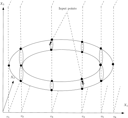
Figure 4. Roadmap of the torus in $\mbox{\rm R}^{3}$.

A key ingredient of the roadmap is the construction of pseudo-critical points and values defined above. The construction of the roadmap of an algebraic set containing a finite number of input points ${\mathcal{N}}$ of this algebraic set is as follows. We first construct $X_{2}$-pseudo-critical points on ${\rm Z}(Q,\mbox{\rm R}^{k})$ in a parametric way along the $X_{1}$-axis by following continuously, as $x$ varies on the $X_{1}$-axis, the $X_{2}$-pseudo-critical points on ${\rm Z}(Q,\mbox{\rm R}^{k})_{x}$. This results in curve segments and their endpoints on ${\rm Z}(Q,\mbox{\rm R}^{k}).$ The curve segments are continuous semi-algebraic curves parametrized by open intervals on the $X_{1}$-axis and their endpoints are points of ${\rm Z}(Q,\mbox{\rm R}^{k})$ above the corresponding endpoints of the open intervals. Since these curves and their endpoints include for every $x\in\mbox{\rm R}$ the $X_{2}-$pseudo-critical points of ${\rm Z}(Q,\mbox{\rm R}^{k})_{x}$, they meet every connected component of ${\rm Z}(Q,\mbox{\rm R}^{k})_{x}$. Thus, the set of curve segments and their endpoints already satisfy ${\rm RM}_{2}.$ However, it is clear that this set might not be semi-algebraically connected in a semi-algebraically connected component and so ${\rm RM}_{1}$ might not be satisfied. We add additional curve segments to ensure connectedness by recursing in certain distinguished hyperplanes defined by $X_{1}=z$ for distinguished values $z$.

The set of distinguished values is the union of the $X_{1}$-pseudo-critical values, the first coordinates of the input points ${\mathcal{N}}$, and the first coordinates of the endpoints of the curve segments. A distinguished hyperplane is an hyperplane defined by $X_{1}=v$, where $v$ is a distinguished value. The input points, the endpoints of the curve segments, and the intersections of the curve segments with the distinguished hyperplanes define the set of distinguished points.

Let the distinguished values be $v_{1}<\ldots<v_{\ell}.$ Note that amongst these are the $X_{1}$-pseudo-critical values. Above each interval $(v_{i},v_{i+1})$ we have constructed a collection of curve segments ${\mathcal{C}}_{i}$ meeting every semi-algebraically connected component of ${\rm Z}(Q,\mbox{\rm R}^{k})_{v}$ for every $v\in(v_{i},v_{i+1})$. Above each distinguished value $v_{i}$ we have a set of distinguished points ${\mathcal{N}}_{i}$. Each curve segment in ${\mathcal{C}}_{i}$ has an endpoint in ${\mathcal{N}}_{i}$ and another in ${\mathcal{N}}_{i+1}$. Moreover, the union of the ${\mathcal{N}}_{i}$ contains ${\mathcal{N}}$.

We then repeat this construction in each distinguished hyperplane $H_{i}$ defined by $X_{1}=v_{i}$ with input $Q(v_{i},X_{2},\ldots,X_{k})$ and the distinguished points in ${\mathcal{N}}_{i}$. Thus, we construct distinguished values $v_{i,1},\ldots,v_{i,\ell(i)}$ of ${\rm Z}(Q(v_{i},X_{2},\ldots,X_{k}),\mbox{\rm R}^{k-1})$ (with the role of $X_{1}$ being now played by $X_{2}$) and the process is iterated until for $I=(i_{1},\ldots,i_{k-2}),1\leq i_{1}\leq\ell,\ldots,1\leq i_{k-2}\leq\ell(i_{1},\ldots,i_{k-3}),$ we have distinguished values $v_{I,1}<\ldots<v_{I,\ell(I)}$ along the $X_{k-1}$ axis with corresponding sets of curve segments and sets of distinguished points with the required incidences between them.

The following theorem is proved in [17] (see also [22]).

Proposition 4.14.

The semi-algebraic set $\mbox{\rm RM}({\rm Z}(Q,\mbox{\rm R}^{k}),{\mathcal{N}})$ obtained by this construction is a roadmap for ${\rm Z}(Q,\mbox{\rm R}^{k})$ containing ${\mathcal{N}}$.

Note that if $x\in{\rm Z}(Q,\mbox{\rm R}^{k})$, $\mbox{\rm RM}({\rm Z}(Q,\mbox{\rm R}^{k}),\{x\})$ contains a path, $\gamma(x)$, connecting a distinguished point $p$ of $\mbox{\rm RM}({\rm Z}(Q,\mbox{\rm R}^{k}))$ to $x$.

4.3.1. The Divergence Property of Connecting Paths

In applications to algorithms for computing Betti numbers of semi-algebraic sets it becomes important to examine the properties of parametrized paths which are the unions of connecting paths starting at a given $p$ and ending at $x$, where $x$ varies over a certain semi-algebraic subset of ${\rm Z}(Q,\mbox{\rm R}^{k})$.

We first note that for any $x=(x_{1},\ldots,x_{k})\in{\rm Z}(Q,\mbox{\rm R}^{k})$ we have by construction that $\mbox{\rm RM}({\rm Z}(Q,\mbox{\rm R}^{k}))$ is contained in $\mbox{\rm RM}({\rm Z}(Q,\mbox{\rm R}^{k}),\{x\})$. In fact,

$$\halign{\hbox to\displaywidth{$\hfil\displaystyle#\hfil$}\cr 0.0pt{\hfil$\displaystyle\mbox{\rm RM}({\rm Z}(Q,\mbox{\rm R}^{k}),\{x\})=\mbox{\rm RM}({\rm Z}(Q,\mbox{\rm R}^{k}))\cup\mbox{\rm RM}({\rm Z}(Q,\mbox{\rm R}^{k})_{x_{1}},{\mathcal{M}}_{x_{1}}),\crcr}}$$

where ${\mathcal{M}}_{x_{1}}$ consists of $(x_{2},\ldots,x_{k})$ and the finite set of points obtained by intersecting the curves in $\mbox{\rm RM}({\rm Z}(Q,\mbox{\rm R}^{k}))$ parametrized by the $X_{1}$-coordinate with the hyperplane $\pi_{1}^{-1}(x_{1})$.

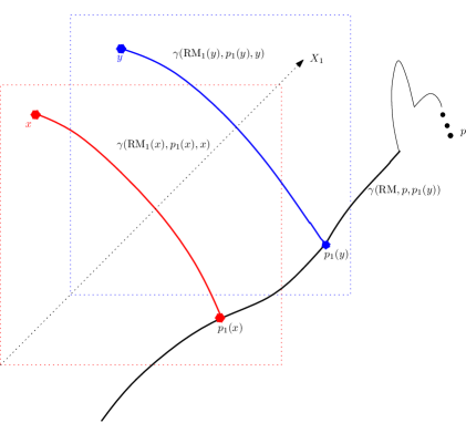
Figure 5. The connecting path $\Gamma(x)$

A connecting path $\gamma(x)$ (with non-self intersecting image) joining a distinguished point $p$ of $\mbox{\rm RM}({\rm Z}(Q,\mbox{\rm R}^{k}))$ to $x$ can be extracted from $\mbox{\rm RM}({\rm Z}(Q,\mbox{\rm R}^{k}),\{x\})$. The connecting path $\gamma(x)$ consists of two consecutive parts, $\gamma_{0}(x)$ and $\Gamma_{1}(x)$. The path $\gamma_{0}(x)$ is contained in $\mbox{\rm RM}({\rm Z}(Q,\mbox{\rm R}^{k}))$ and the path $\Gamma_{1}(x)$ is contained in ${\rm Z}(Q,\mbox{\rm R}^{k})_{x_{1}}$. The part $\gamma_{0}(x)$ consists of a sequence of sub-paths $\gamma_{0,0},\ldots,\gamma_{0,m}$. Each $\gamma_{0,i}$ is a semi-algebraic path parametrized by one of the co-ordinates $X_{1},\ldots,X_{k}$, over some interval $[a_{0,i},b_{0,i}]$ with $\gamma_{0,0}(a_{0,0})=p$. The semi-algebraic maps $\gamma_{0,0},\ldots,\gamma_{0,m}$ and the end-points of their intervals of definition $a_{0,0},b_{0,0},\ldots,a_{0,m},b_{0,m}$ are all independent of $x$ (up to the discrete choice of the path $\gamma(x)$ in $\mbox{\rm RM}({\rm Z}(Q,\mbox{\rm R}^{k}),\{x\})$), except $b_{0,m}$ which depends on $x_{1}$.

Moreover, $\Gamma_{1}(x)$ can again be decomposed into two parts $\gamma_{1}(x)$ and $\Gamma_{2}(x)$ with $\Gamma_{2}(x)$ contained in ${\rm Z}(Q,\mbox{\rm R}^{k})_{(x_{1},x_{2})}$ and so on.

If $y=(y_{1},\ldots,y_{k})\in{\rm Z}(Q,\mbox{\rm R}^{k})$ is another point such that $x_{1}\neq y_{1}$, then since ${\rm Z}(Q,\mbox{\rm R}^{k})_{x_{1}}$ and ${\rm Z}(Q,\mbox{\rm R}^{k})_{y_{1}}$ are disjoint, it is clear that

$$\mbox{\rm RM}({\rm Z}(Q,\mbox{\rm R}^{k}),\{x\})\cap\mbox{\rm RM}({\rm Z}(Q,\mbox{\rm R}^{k}),\{y\})=\mbox{\rm RM}({\rm Z}(Q,\mbox{\rm R}^{k})).$$

Now consider a connecting path $\gamma(y)$ extracted from $\mbox{\rm RM}({\rm Z}(Q,\mbox{\rm R}^{k}),\{y\})$. The images of $\Gamma_{1}(x)$ and $\Gamma_{1}(y)$ are disjoint. If the image of $\gamma_{0}(y)$ (which is contained in $\mbox{\rm RM}({\rm Z}(Q,\mbox{\rm R}^{k})$) follows the same sequence of curve segments as $\gamma_{0}(x)$ starting at $p$ (i.e. it consists of the same curves segments $\gamma_{0,0},\ldots,\gamma_{0,m}$ as in $\gamma_{0}(x)$), then it is clear that the images of the paths $\gamma(x)$ and $\gamma(y)$ has the property that they are identical up to a point and they are disjoint after it. This is called the divergence property in [20].

4.3.2. Roadmaps of General Semi-algebraic Sets

Using the same ideas as above and some additional techniques for controlling the combinatorial complexity of the algorithm it is possible to extend the roadmap algorithm to the case of semi-algebraic sets. The following theorem appears in [17, 22] and gives the most efficient algorithm for constructing roadmaps.

Theorem 4.15.

[17, 22] Let $Q\in{\mbox{\rm R}}[X_{1},\ldots,X_{k}]$ with ${\rm Z}(Q,\mbox{\rm R}^{k})$ of dimension $k^{\prime}$ and let ${\mathcal{P}}\subset{\mbox{\rm R}}[X_{1},\ldots,X_{k}]$ be a set of at most $s$ polynomials for which the degrees of the polynomials in ${\mathcal{P}}$ and $Q$ are bounded by $d.$ Let $S$ be a ${\mathcal{P}}$-semi-algebraic subset of ${\rm Z}(Q,\mbox{\rm R}^{k})$. There is an algorithm which computes a roadmap $\mbox{\rm RM}(S)$ for $S$ with complexity $s^{k^{\prime}+1}d^{O(k^{2})}$ in the ring D generated by the coefficients of $Q$ and the elements of ${\mathcal{P}}$. If $\mbox{\rm D}={\mathbb{Z}},$ and the bit-sizes of the coefficients of the polynomials are bounded by $\tau$, then the bit-sizes of the integers appearing in the intermediate computations and the output are bounded by $\tau d^{O(k^{2})}$.

Theorem 4.15 immediately implies that there is an algorithm whose output is exactly one point in every semi-algebraically connected component of $S$ and whose complexity in the ring generated by the coefficients of $Q$ and ${\mathcal{P}}$ is bounded by $s^{k^{\prime}+1}d^{O(k^{2})}$. In particular, this algorithm counts the number semi-algebraically connected component of $S$ within the same time bound.

5. Topological Preliminaries

The purpose of this section is to provide a self-contained introduction to the basic mathematical machinery needed later. Some of the topics would be familiar to most readers while a few others perhaps less so. The sophisticated reader can choose to skip this whole section and proceed directly to the descriptions of the various algorithms in the later sections.

We give a brief review of the concepts from algebraic topology that play a role in the results surveyed in this paper. These include the definition of complexes of vector spaces (Section 5.2.1), definition of cohomology groups of semi-algebraic sets (Section 5.3), properties of the Euler-Poincaré characteristic of semi-algebraic sets 5.3.1), the nerve complex of covers (Section 5.5), a generalization of the nerve complex (Section 5.6), the Mayer-Vietoris double complex and its associated spectral sequence (Section 5.7), the descent spectral sequence (Section 5.8), and the properties of homotopy colimits (Section 5.9).

5.1. Homology and Cohomology groups

Before we get to the precise definitions of these groups it is good to have some intuition about them. As noted before closed and bounded semi-algebraic sets are finitely triangulable. This means that each closed and bounded semi-algebraic set $S\subset\mbox{\rm R}^{k}$ is homeomorphic (in fact, by a semi-algebraic map) to the polyhedron $|K|$ associated to a finite simplicial complex $K$. In fact $K$ can be chosen such that $|K|\subset\mbox{\rm R}^{k}$, and there is an effective algorithm (see Theorem 4.5) for computing $K$ given $S$. The simplicial cohomology (resp. homology groups) of $S$ are defined in terms of $K$ and are well-defined (i.e they are independent of the chosen triangulation which is of course very far from being unique).

Roughly speaking the simplicial homology groups of a finite simplicial complex $K$ with coefficients in a field ${\mathbb{F}}$ (which we assume to be ${\mathbb{Q}}$ in this survey) are finite dimensional ${\mathbb{F}}$-vector spaces and measure the connectivity of $|K|$ in various dimensions. For example, the zero-th simplicial homology group, ${\rm H}_{0}(K)$, has a generator corresponding to each connected component of $K$ and its dimension gives the number of connected components of $|K|$. Similarly the first simplicial homology group, ${\rm H}_{1}(K)$, is generated by the “one-dimensional holes” of $|K|$, and its dimension is the number of “independent” one-dimensional holes of $|K|$. If $K$ is one-dimensional (that is a finite graph) the dimension of ${\rm H}_{1}(K)$ is the number of independent cycles in $K$. Analogously, the $i$-th the simplicial homology group, ${\rm H}_{i}(K)$, is generated by the “$i$-dimensional holes” of $|K|$, and its dimension is the number of independent $i$-dimensional holes of $|K|$. Intuitively an $i$-dimensional hole is an $i$-dimensional closed surface in $K$ (technically called a cycle) which does not bound any $(i+1)$-dimensional subset of $|K|$.

The simplicial cohomology groups of $K$ are dual (and isomorphic) to the simplicial homology groups of $K$ as groups. However, in addition to the group structure they also carry a multiplicative structure (the so called cup-product) which makes them a finer topological invariant than the homology groups. We are not going to use this multiplicative structure. Cohomology groups also have nice but less geometric interpretations. Roughly speaking the cohomology groups of $K$ represent spaces of globally defined objects satisfying certain local conditions. For example, the zero-th cohomology group, ${\rm H}^{0}(K)$, can be interpreted as the vector space of global functions on $|K|$ which are locally constant. It is easy to see from this interpretation that the dimension of ${\rm H}^{0}(K)$ is the number of connected components of $K$. Similar geometric interpretations can be given for the higher cohomology groups, in terms of vector spaces of (globally defined) differential forms satisfying certain local condition (of being closed). In literature this cohomology theory is referred to as de Rham cohomology theory and it is usually defined for smooth manifolds, but it can also be defined for simplicial complexes (see for example [54, Section 1.3.1]).

5.1.1. Homology vs Cohomology

It turns out that the cohomological point of view gives better intuition in designing algorithms described later in the paper. This is our primary reason behind preferring cohomology over homology. Another reason for preferring the cohomology groups over the homology groups is that their interpretations continue to make sense in applications outside of semi-algebraic geometry where the notions of holes is meaningless (for instance, think of algebraic varieties defined over fields of positive characteristics) but the notion of global functions (or for instance differential forms) continue to make sense.

5.2. Definition of the Cohomology Groups of a Simplicial Complex

We now give precise definitions of the cohomology groups of simplicial complexes.

In order to do so we first need to introduce some amount of algebraic machinery – namely the concept of complexes of vector spaces and homomorphisms between them.

5.2.1. Complex of Vector Spaces

A complex of vector spaces is just a sequence of vector spaces and linear transformations satisfying the property that the composition of two successive linear transformations is $0$.

More precisely

Definition 5.1 (Complex of Vector Spaces).

A sequence $\{{\rm C}^{p}\}$, $p\in{\mathbb{Z}}$, of ${\mathbb{Q}}$-vector spaces together with a sequence $\{\delta^{p}\}$ of homomorphisms $\delta^{p}:{\rm C}^{p}\rightarrow{\rm C}^{p+1}$ (called differentials) for which

(5.1) $$\delta^{p+1}\circ\delta^{p}=0$$

for all $p$ is called a complex.

The most important example for us of a complex of vector spaces is the co-chain complex of a simplicial complex $K$ denoted by ${\rm C}^{\bullet}(K)$. It is defined as follows.

Definition 5.2 (Simplicial cochain complex).

For each $p\geq 0$, ${\rm C}^{p}(K)$ is a linear functional on the ${\mathbb{Q}}$-vector-space generated by the $p$-simplices of $K$. Given $\phi\in{\rm C}^{p}(K)$, $\delta^{p}(\phi)$ is specified by its values on the $(p+1)$-dimensional simplices of $K$. Given a $(p+1)$-dimensional simplex $\sigma=[a_{0},\ldots,a_{p+1}]$ of $K$

(5.2) $$(\delta^{p}\phi)([a_{0},\ldots,a_{p+1}])=\sum_{i=0}^{p+1}(-1)^{i}\phi([a_{0},\ldots,\hat{a_{i}},\ldots,a_{p+1}]),$$

where $\hat{}$ denotes omission.

Notice that each $[a_{0},\ldots,\hat{a_{i}},\ldots,a_{p+1}]$ is a $p$-dimensional simplex of $K$ and since $\phi\in{\rm C}^{p}(K)$, $\phi([a_{0},\ldots,\hat{a_{i}},\ldots,a_{p+1}])\in{\mathbb{Q}}$ is well-defined. It is an exercise now to check that the homomorphisms $\delta^{p}:{\rm C}^{p}(K)\rightarrow{\rm C}^{p+1}(K)$ indeed satisfy Eqn. 5.1 in the definition of a complex.

Now let $K$ be a simplicial complex and $L\subset K$ a sub-complex of $K$ – we will denote such a pair simply by $(K,L)$. Then for each $p\geq 0$ we have that ${\rm C}^{p}(L)\subset{\rm C}^{p}(K)$ and we denote by ${\rm C}^{p}(K,L)$ the quotient space ${\rm C}^{p}(K)/{\rm C}^{p}(L)$. It is now an easy exercise to verify that the differentials $\delta^{p}$ in the complex ${\rm C}^{p}(K)$ descend to ${\rm C}^{p}(K,L)$ and we define

Definition 5.3 (Simplicial cochain complex of a pair).

The simplicial cochain complex of the pair $(K,L)$ to be the complex ${\rm C}^{\bullet}(K,L)$ whose terms, ${\rm C}^{p}(K,L)$, and differentials, $\delta^{p}$, are defined as above.

Often, particularly in the context of algorithmic applications it is more economical to use cellular complexes instead of simplicial complexes. We recall here the definition of a finite regular cell complex referring the reader to standard sources in algebraic topology for more in-depth study of cellular theory (see [69, pp. 81]).

Definition 5.4 (Regular cell complex).

An $\ell$-dimensional cell in $\mbox{\rm R}^{k}$ is a subset of $\mbox{\rm R}^{k}$ homeomorphic to $\overline{B_{\ell}(0,1)}$. A regular cell complex $\Sigma$ in $\mbox{\rm R}^{k}$ is a finite collection of cells satisfying the following properties:

1. If $c_{1},c_{2}\in\Sigma$, then either $c_{1}\cap c_{2}=\emptyset$ or $c_{1}\subset\partial c_{2}$ or $c_{2}\subset\partial c_{1}$.

2. The boundary of each cell of $\Sigma$ is a union of cells of $\Sigma$.

We denote by $|\Sigma|$ the set $\displaystyle{\bigcup_{c\in\Sigma}c}.$

Remark 5.5.

Notice that every simplicial complex $K$ may be considered as a regular cell complex whose cells are the closures of the simplices of $K$.

As in the case of simplicial complexes it is possible to associate a complex, ${\rm C}^{\bullet}(\Sigma)$ (the co-chain complex of $K$), to each regular cell complex $K$ which is defined in an analogous manner. In order to avoid technicalities we omit the precise definition of this complex referring the interested reader to [69, pp. 82] instead. We remark that the dimension of ${\rm C}^{p}(\Sigma)$ is equal to the number of $p$-dimensional cells in $\Sigma$ and the matrix entries for the differentials in the complex with respect to the standard basis comes from $\{0,1,-1\}$ just as in the case of simplicial co-chain complexes.

The advantage of using cell complexes instead of simplicial complexes can be seen in the following example.

Example 5.6.

Consider the unit sphere $\mbox{${\bf S}$}^{k}\subset\mbox{\rm R}^{k+1}$. For $0\leq j\leq k+1$ and ${\varepsilon}\in\{+,-\}$ let

(5.3) $$c_{j}^{{\varepsilon}}=\{x\in\mbox{${\bf S}$}^{k}\;\mid\;X_{0}=\cdots=X_{j-1}=0,{\varepsilon}X_{j}\geq 0\}.$$

Then it is easy to check that each $c_{j}^{{\varepsilon}}$ is a $k-j$ dimensional cell and the collection, $\displaystyle{\Sigma_{k}=\{c_{j}^{{\varepsilon}}\;\mid\;0\leq j\leq k,{\varepsilon}\in\{-,+\}\}}$ is a regular cell complex with $|\Sigma_{k}|=\mbox{${\bf S}$}^{k}$ (see Figure 6 for the case $k=2$).

Figure 6. Cell decomposition of $\mbox{${\bf S}$}^{2}$

Notice that $\#\Sigma_{k}=2k$. On the other hand if we consider the sphere as homeomorphic to the boundary of a standard $(k+1)$-dimensional simplex, then the corresponding simplicial complex will contain $(2^{k+2}-2)$ simplices (which is exponentially large in $k$).

We now associate to each complex, ${\rm C}^{\bullet}$, a sequence of vector spaces, ${\rm H}^{p}({\rm C}^{\bullet})$, called the cohomology groups of ${\rm C}^{\bullet}$. Note that it follows from Eqn. 5.1 that for a complex ${\rm C}^{\bullet}$ with differentials $\delta^{p}:{\rm C}^{p}\rightarrow{\rm C}^{p+1}$ the subspace $B^{p}({\rm C}^{\bullet})={\rm Im}(\delta^{p-1})\subset{\rm C}^{p}$ is contained in the subspace $Z^{p}({\rm C}^{\bullet})=\mbox{\rm Ker}(\delta^{p})\subset{\rm C}^{p}$. The subspaces $B^{p}({\rm C}^{\bullet})$ (resp. $Z^{p}({\rm C}^{\bullet})$) are usually referred to as the co-boundaries (resp. co-cycles) of the complex ${\rm C}^{\bullet}$. Moreover,

Definition 5.7 (Cohomology groups of a complex).

The cohomology groups, ${\rm H}^{p}({\rm C}^{\bullet})$, are defined by

(5.4) $${\rm H}^{p}({\rm C}^{\bullet})={Z^{p}({\rm C}^{\bullet})}/{B^{p}({\rm C}^{\bullet})}.$$

We will denote by ${\rm H}^{*}({\rm C}^{\bullet})$ the graded vector space $\bigoplus_{p}{\rm H}^{p}({\rm C}^{\bullet})$.

Note that the cohomology groups, ${\rm H}^{p}({\rm C}^{\bullet})$, are all ${\mathbb{Q}}$-vector spaces (finite dimensional if the vector spaces ${\rm C}^{p}$’s are themselves finite dimensional).

Definition 5.8 (Exact sequence).

A complex ${\rm C}^{\bullet}$ is called acyclic and the corresponding sequence of vector space homomorphisms is called an exact sequence if ${\rm H}^{*}({\rm C}^{\bullet})=0$.

Applying Definition 5.7 to the particular case of the co-chain complex of a simplicial complex $K$ (cf. Definition 5.2) we obtain

5.2.2. Cohomology of a Simplicial Complex

Definition 5.9 (Cohomology of a simplicial complex).

The cohomology groups of a simplicial complex $K$ are by definition the cohomology groups, ${\rm H}^{p}({\rm C}^{\bullet}(K))$, of its co-chain complex.

Similarly, given a pair of simplicial complexes $(K,L)$, we define

Definition 5.10 (Cohomology of a pair).

The cohomology groups of the pair $(K,L)$ are by definition the cohomology groups, ${\rm H}^{p}({\rm C}^{\bullet}(K,L))$, of its co-chain complex.

Example 5.11.

Let $\Delta_{n}$ be the simplicial complex corresponding to an $n$-simplex. In other words the simplices of $\Delta_{n}$ consist of $[i_{0},\ldots,i_{\ell}],0\leq i_{0}<\cdots<i_{\ell}\leq n$. The polyhedron $|\Delta_{n}|$ is just the $n$-dimensional simplex. Then using Definition 5.9 one can verify that

$${\rm H}^{i}(\Delta_{n}) ={\mathbb{Q}},\;i=0,$$

$${\rm H}^{i}(\Delta_{n}) =0,\;i>0.$$

Example 5.12.

Let $\partial\Delta_{n}$ be the simplicial complex corresponding to the boundary of the $n$-simplex. In other words the simplices of $\partial\Delta_{n}$ consist of $[i_{0},\ldots,i_{\ell}],0\leq i_{0}<\cdots<i_{\ell}\leq n,\ell<n$. Then again by a direct application of Definition 5.9 one can verify that

$${\rm H}^{i}(\partial\Delta_{n}) ={\mathbb{Q}},\;i=0,n-1$$

$${\rm H}^{i}(\partial\Delta_{n}) =0,\;\mbox{ else}.$$

The above examples serve to confirm our geometric intuition behind the homology groups of the spaces $|\Delta_{n}|$ and $|\partial\Delta_{n}|$ explained in Section 5.1 above – namely that they are both connected and $|\Delta_{n}|$ has no holes in dimension $>0$, and $|\partial\Delta_{n}|$ has a single $(n-1)$-dimensional hole.

Example 5.13.

It is also an useful exercise to verify that

$${\rm H}^{i}(\Delta_{n},\partial\Delta_{n}) ={\mathbb{Q}},\;i=0,n$$

$${\rm H}^{i}(\Delta_{n},\partial\Delta_{n}) =0,\;\mbox{ else}.$$

Remark 5.14.

Example 5.13 illustrates that for “nice spaces” of the kind we consider in this paper (such as regular cell complexes) the cohomology groups of a pair $(K,L)$ are isomorphic to the cohomology groups of the quotient space $|K|/|L|$. For instance, the above example illustrates the fact that the topological quotient of an $n$-dimensional ball by its boundary is the $n$-dimensional sphere.

5.2.3. Homomorphisms of Complexes

We will also need the notion of homomorphisms of complexes which generalizes the notion of ordinary vector space homomorphisms.

Definition 5.15 (Homomorphisms of complexes).

Given two complexes, ${\rm C}^{\bullet}=({\rm C}^{p},\delta^{p})$ and $\mbox{\rm D}^{\bullet}=(\mbox{\rm D}^{p},\delta^{p})$, a homomorphism of complexes, $\phi^{\bullet}:{\rm C}^{\bullet}\rightarrow\mbox{\rm D}^{\bullet}$, is a sequence of homomorphisms $\phi^{p}:{\rm C}^{p}\rightarrow\mbox{\rm D}^{p}$ for which $\delta^{p}\circ\phi^{p}=\phi^{p+1}\circ\delta^{p}$ for all $p$.

In other words the following diagram is commutative.

(5.5) $$\begin{diagram}$$

A homomorphism of complexes $\phi^{\bullet}:{\rm C}^{\bullet}\rightarrow\mbox{\rm D}^{\bullet}$ induces homomorphisms $\phi^{i}:{\rm H}^{i}({\rm C}^{\bullet})\rightarrow{\rm H}^{i}(\mbox{\rm D}^{\bullet})$ and we will denote the corresponding homomorphism between the graded vector spaces ${\rm H}^{*}({\rm C}^{\bullet}),{\rm H}^{*}(\mbox{\rm D}^{\bullet})$ by $\phi^{*}$.

Definition 5.16 (Quasi-isomorphism).

The homomorphism $\phi^{\bullet}$ is called a quasi-isomorphism if the homomorphism $\phi^{*}$ is an isomorphism.

Having introduced the algebraic machinery of complexes of vector spaces, we now define the cohomology groups of semi-algebraic sets in terms of their triangulations and their associated simplicial complexes.

5.3. Cohomology Groups of Semi-algebraic Sets

A closed and bounded semi-algebraic set $S\subset\mbox{\rm R}^{k}$ is semi-algebraically triangulable (see Theorem 4.5 above).

Definition 5.17 (Cohomology groups of closed and bounded semi-algebraic sets).

Given a triangulation, $h:|K|\rightarrow S$, where $K$ is a simplicial complex, we define the $i$-th simplicial cohomology group of $S$, by ${\rm H}^{i}(S)={\rm H}^{i}({\rm C}^{\bullet}(K))$, where ${\rm C}^{\bullet}(K)$ is the co-chain complex of $K$. The groups ${\rm H}^{i}(S)$ are invariant under semi-algebraic homeomorphisms (and they coincide with the corresponding singular cohomology groups when $\mbox{\rm R}=\mbox{${\mathbb{R}}$}$). We denote by $b_{i}(S)$ the $i$-th Betti number of $S$ (i.e. the dimension of ${\rm H}^{i}(S)$ as a vector space).

Remark 5.18.

For a closed but not necessarily bounded semi-algebraic set $S\subset\mbox{\rm R}^{k}$ we will denote by ${\rm H}^{i}(S)$ the $i$-th simplicial cohomology group of $S\cap\overline{B_{k}(0,r)}$ for sufficiently large $r>0$. The sets $S\cap\overline{B_{k}(0,r)}$ are semi-algebraically homeomorphic for all sufficiently large $r>0$ and hence this definition makes sense. (The last property is usually referred to as the local conic structure at infinity of semi-algebraic sets [22, Theorem 5.48]). The definition of cohomology groups of arbitrary semi-algebraic sets in $\mbox{\rm R}^{k}$ requires some care and several possibilities exist and we refer the reader to [22, Section 6.3] where one such definition is given which agrees with singular cohomology in case $\mbox{\rm R}=\mbox{${\mathbb{R}}$}$.

5.3.1. The Euler-Poincaré Characteristic: Definition and Basic Properties

An useful topological invariant of semi-algebraic sets which is often easier to compute than their Betti numbers is the Euler-Poincaré characteristic.

Definition 5.19 (Euler-Poincaré characteristic of a closed and bounded semi-algebraic set).

Let $S\subset\mbox{\rm R}^{k}$, be a closed and bounded semi-algebraic set. Then the Euler-Poincaré characteristic of $S$ is defined by

(5.6) $$\chi(S)=\sum_{i\geq 0}(-1)^{i}b_{i}(S).$$

From the point of view of designing algorithms, it is useful to define Euler-Poincaré characteristic also for locally closed semi-algebraic sets. A semi-algebraic set is locally closed if it is the intersection of a closed semi-algebraic set with an open one. A standard example of a locally closed semi-algebraic set is the realization, ${\mathcal{R}}(\sigma)$, of a sign-condition $\sigma$ on a family of polynomials.

We now define Euler-Poincaré characteristic for locally closed semi-algebraic sets in terms of the Borel-Moore cohomology groups of such sets (defined below). This definition agrees with the definition of Euler-Poincaré characteristic stated above for closed and bounded semi-algebraic sets. They may be distinct for semi-algebraic sets which are closed but not bounded.

Definition 5.20.

The simplicial cohomology groups of a pair of closed and bounded semi-algebraic sets $T\subset S\subset\mbox{\rm R}^{k}$ are defined as follows. Such a pair of closed and bounded semi-algebraic sets can be triangulated (cf. Theorem 4.5) using a pair of simplicial complexes $(K,A)$ where $A$ is a sub-complex of $K$. The $p$-th simplicial cohomology group of the pair $(S,T)$, ${\rm H}^{p}(S,T)$, is by definition to be ${\rm H}^{p}(K,A)$. The dimension of ${\rm H}^{p}(S,T)$ as a ${\mathbb{Q}}$-vector space is called the $p$-th Betti number of the pair $(S,T)$ and denoted $b_{p}(S,T)$. The Euler-Poincaré characteristic of the pair $(S,T)$ is

$$\chi(S,T)=\sum_{i}(-1)^{i}b_{i}(S,T).$$

Definition 5.21 (Borel-Moore cohomology group).

The $p$-th Borel-Moore cohomology group of $S\subset\mbox{\rm R}^{k}$, denoted ${\rm H}^{p}_{BM}(S)$, is defined in terms of the cohomology groups of a pair of closed and bounded semi-algebraic sets as follows. For any $r>0$ let $S_{r}=S\cap B_{k}(0,r)$. Note that for a locally closed semi-algebraic set $S$ both $\overline{S_{r}}$ and $\overline{S_{r}}\setminus S_{r}$ are closed and bounded, and hence ${\rm H}^{p}(\overline{S_{r}},\overline{S_{r}}\setminus S_{r})$ is well defined. Moreover, it is a consequence of the local conic structure at infinity of semi-algebraic sets (see Remark 5.18 above) that the cohomology group $H^{p}(\overline{S_{r}},\overline{S_{r}}\setminus S_{r})$ is invariant for all sufficiently large $r>0$. We define ${\rm H}^{p}_{BM}(S)={\rm H}^{p}(\overline{S_{r}},\overline{S_{r}}\setminus S_{r})$ for $r>0$ sufficiently large and it follows from the above remark that it is well defined.

The Borel-Moore cohomology groups are invariant under semi-algebraic homeomorphisms (see [25]. It also follows clearly from the definition that for a closed and bounded semi-algebraic set the Borel-Moore cohomology groups coincide with the simplicial cohomology groups.

Definition 5.22 (Borel-Moore Euler-Poincaré characteristic).

For a locally closed semi-algebraic set $S$ we define the Borel-Moore Euler-Poincaré characteristic by

(5.7) $$\chi^{BM}(S)=\sum_{i=0}^{k}(-1)^{i}~{}b_{i}^{BM}(S)$$

where $b_{i}^{BM}(S)$ denotes the dimension of ${\rm H}^{i}_{BM}(S).$

Since the Borel-Moore Euler-Poincaré characteristic might not be very familiar, the reader is encouraged to compute it in a few simple examples. In particular, one should check that for the half-open interval $[0,1)$ which is locally closed we have

(5.8) $$\chi^{BM}([0,1))=0.$$

We also have

(5.9) $$\chi^{BM}((0,1))=-1,$$

and more generally,

(5.10) $$\chi^{BM}(B_{k}(0,1))=(-1)^{k}.$$

If $S$ is closed and bounded then $\chi^{BM}(S)=\chi(S)$.

The Borel-Moore Euler-Poincaré characteristic has the following additivity property (reminiscent of the similar property of volumes) which makes them particularly useful in algorithmic applications (see for example Section 7.3 below).

Proposition 5.23.

Let $X,X_{1}$ and $X_{2}$ be locally closed semi-algebraic sets such that

$$X_{1}\cup X_{2}=X,X_{1}\cap X_{2}=\emptyset.$$

Then

(5.11) $$\chi^{BM}(X)=\chi^{BM}(X_{1})+\chi^{BM}(X_{2}).$$

Since for closed and bounded semi-algebraic sets, the Borel-Moore Euler-Poincaré characteristic agrees with the ordinary Euler-Poincaré characteristic, it is easy to derive the following additivity property of the Euler-Poincaré characteristic of closed and bounded sets.

Proposition 5.24.

Let $X_{1}$ and $X_{2}$ be closed and bounded semi-algebraic sets. Then

(5.12) $$\chi(X_{1}\cup X_{2})=\chi(X_{1})+\chi(X_{2})-\chi(X_{1}\cap X_{2}).$$

Note that Proposition 5.24 is an immediate consequence of Proposition 5.23 once we notice that the sets $Y_{1}=X_{1}\setminus(X_{1}\cap X_{2})$ and $Y_{2}=X_{2}\setminus(X_{1}\cap X_{2})$ are locally closed, the set $X_{1}\cup X_{2}$ is the disjoint union of the locally closed sets $Y_{1},Y_{2}$ and $X_{1}\cap X_{2}$, and

$$\chi^{BM}(Y_{i})=\chi^{BM}(X_{i})-\chi^{BM}(X_{1}\cap X_{2})=\chi(X_{i})-\chi(X_{1}\cap X_{2}),\mbox{ for }i=1,2.$$

More generally by applying Proposition 5.24 inductively we get the following inclusion-exclusion property of the (ordinary) Euler-Poincaré characteristic.

For any $n\in{\mathbb{Z}}_{\geq 0}$ we denote by $[n]$ the set $\{1,\ldots,n\}$.

Proposition 5.25.

Let $X_{1},\ldots,X_{n}$ be closed and bounded semi-algebraic sets. Then denoting by $X_{I}$ the semi-algebraic set $\displaystyle{\bigcap_{i\in I}X_{i}}$ for $I\subset[n]$, we have

(5.13) $$\chi(\bigcup_{i\in[n]}X_{i})=\sum_{I\subset[n]}(-1)^{(\#I+1)}~{}\chi(X_{I}).$$

5.4. Homotopy Invariance

The cohomology groups of semi-algebraic sets as defined above (Definition 5.17) are obviously invariant under semi-algebraic homeomorphisms. But, in fact, they are invariant under a weaker equivalence relation – namely, semi-algebraic homotopy equivalence (defined below). This property is crucial in the design of efficient algorithms for computing Betti numbers of semi-algebraic sets since it allows us to replace a given set by one that is better behaved from the algorithmic point of view but having the same homotopy type as the original set. This technique is ubiquitous in algorithmic semi-algebraic geometry and we will see some version of it in almost every algorithm described in the following sections (cf. Example 4.11).

Remark 5.26.

The reason behind insisting on the prefix “semi-algebraic” with regard to homeomorphisms and homotopy equivalences here and in the rest of the paper, is that for general real closed fields, the ordinary Euclidean topology could be rather strange. For example, the real closed field, $\mbox{${\mathbb{R}}$}_{{\rm alg}}$, of real algebraic numbers is totally disconnected as a topological space under the Euclidean topology. On the other hand, if the ground field $\mbox{\rm R}=\mbox{${\mathbb{R}}$}$, then we can safely drop the prefix “semi-algebraic” in the statements made above. However, even if we start with $\mbox{\rm R}=\mbox{${\mathbb{R}}$}$, in many applications described below we enlarge the field by taking non-archimedean extensions of R (see Section 4.2.1), and the remarks made above would again apply to these field extensions.

Definition 5.27 (Semi-algebraic homotopy).

Let $X,Y$ be two closed and bounded semi-algebraic sets. Two semi-algebraic continuous functions $f,g:X\rightarrow Y$ are semi-algebraically homotopic, $f\sim_{sa}g$, if there is a continuous semi-algebraic function $F:X\times[0,1]\rightarrow Y$ such that $F(x,0)=f(x)$ and $F(x,1)=g(x)$ for all $x\in X$.

Clearly, semi-algebraic homotopy is an equivalence relation among semi-algebraic continuous maps from $X$ to $Y$.

Definition 5.28 (Semi-algebraic homotopy equivalence).

The sets $X,Y$ are semi-algebraically homotopy equivalent if there exist semi-algebraic continuous functions $f:X\rightarrow Y$, $g:Y\rightarrow X$ such that $g\circ f\sim_{sa}{\rm Id}_{X}$, $f\circ g\sim_{sa}{\rm Id}_{Y}$.

We have

Proposition 5.29 (Homotopy Invariance of the Cohomology Groups).

Let $X,Y$ be two closed and bounded semi-algebraic sets of $\mbox{\rm R}^{k}$ that are semi-algebraically homotopy equivalent. Then, ${\rm H}^{*}(X)\cong{\rm H}^{*}(Y)$.

5.5. The Leray Property and the Nerve Lemma

It clear from the definition of the cohomology groups of closed and bounded semi-algebraic sets (Definition 5.17 above) the Betti numbers of such a set can be computed using elementary linear algebra once we have a triangulation of the set. However, as we have seen before (cf. Theorem 4.5), triangulations of semi-algebraic sets are expensive to compute, requiring double exponential time.

One basic idea that underlies some of the recent progress in designing algorithms for computing the Betti numbers of semi-algebraic sets is that the cohomology groups of a semi-algebraic set can often be computed from a sufficiently well-behaved covering of the set without having to triangulate the set.

The idea of computing cohomology from “good” covers is an old one in algebraic topology and the first result in this direction is often called the “Nerve Lemma”. In this section we give a brief introduction to the Nerve Lemma and its generalizations.

We first define formally the notion of a cover of a closed, bounded semi-algebraic set.

Definition 5.30 (Cover).

Let $S\subset\mbox{\rm R}^{k}$ be a closed and bounded semi-algebraic set. A cover, ${\mathcal{C}}(S)$, of $S$ consists of an ordered index set, which by a slight abuse of language we also denote by ${\mathcal{C}}(S)$, and a map that associates to each $\alpha\in{\mathcal{C}}(S)$ a closed and bounded semi-algebraic subset $S_{\alpha}\subset S$ such that

$$S=\bigcup_{\alpha\in{\mathcal{C}}(S)}S_{\alpha}.$$

Remark 5.31.

Even though the notation for a cover might seem unnecessarily heavy at the moment it will prove useful later on the paper when we discuss non-Leray covers (see Section 5.6 below).

For $\alpha_{0},\ldots,\alpha_{p},\in{\mathcal{C}}(S)$, we associate to the formal product, $\alpha_{0}\cdots\alpha_{p}$, the closed and bounded semi-algebraic set

(5.14) $$S_{\alpha_{0}\cdots\alpha_{p}}=S_{\alpha_{0}}\cap\cdots\cap S_{\alpha_{p}}.$$

Recall that the $0$-th simplicial cohomology group of a closed and bounded semi-algebraic set $X$, ${\rm H}^{0}(X)$, can be identified with the ${\mathbb{Q}}$-vector space of ${\mathbb{Q}}$-valued locally constant functions on $X$. Clearly the dimension of ${\rm H}^{0}(X)$ is equal to the number of connected components of $X$.

For $\alpha_{0},\alpha_{1},\ldots,\alpha_{p},\beta\in{\mathcal{C}}(S)$, and $\beta\not\in\{\alpha_{0},\ldots,\alpha_{p}\}$, let

$$r_{\alpha_{0},\ldots,\alpha_{p};\beta}:{\rm H}^{0}(S_{\alpha_{0}\cdots\alpha_{p}})\longrightarrow{\rm H}^{0}(S_{\alpha_{0}\cdots\alpha_{p}\cdot\beta})$$

be the homomorphism defined as follows. Given a locally constant function, $\phi\in{\rm H}^{0}(S_{\alpha_{0}\cdots\alpha_{p}})$, $r_{\alpha_{0}\cdots\alpha_{p};\beta}(\phi)$ is the locally constant function on $S_{\alpha_{0}\cdots\alpha_{p}\cdot\beta}$ obtained by restricting $\phi$ to $S_{\alpha_{0}\cdots\alpha_{p}\cdot\beta}$.

We define the generalized restriction homomorphisms

$$\delta^{p}:\bigoplus_{\alpha_{0}<\cdots<\alpha_{p},\alpha_{i}\in{\mathcal{C}}(S)}{\rm H}^{0}(S_{\alpha_{0}\cdots\alpha_{p}})\longrightarrow\bigoplus_{\alpha_{0}<\cdots<\alpha_{p+1},\alpha_{i}\in{\mathcal{C}}(S)}{\rm H}^{0}(S_{\alpha_{0}\cdots\alpha_{p+1}})$$

by

(5.15) $$\delta^{p}(\phi)_{\alpha_{0}\cdots\alpha_{p+1}}=\sum_{0\leq i\leq p+1}(-1)^{i}r_{\alpha_{0}\cdots\hat{\alpha_{i}}\cdots\alpha_{p+1};\alpha_{i}}(\phi_{\alpha_{0}\cdots\hat{\alpha_{i}}\cdots\alpha_{p+1}}),$$

where $\phi\in\bigoplus_{\alpha_{0}<\cdots<\alpha_{p}\in{\mathcal{C}}(S)}{\rm H}^{0}(S_{\alpha_{0}\cdots\alpha_{p}})$ and $r_{\alpha_{0}\cdots\hat{\alpha_{i}}\cdots\alpha_{p+1};\alpha_{i}}$ is the restriction homomorphism defined previously. The sequence of homomorphisms $\delta^{p}$ gives rise to a complex, ${\rm L}^{\bullet}({\mathcal{C}}(S))$, defined by

(5.16) $${\rm L}^{p}({\mathcal{C}}(S))=\bigoplus_{\alpha_{0}<\cdots<\alpha_{p},\alpha_{i}\in{\mathcal{C}}(S)}{\rm H}^{0}(S_{\alpha_{0}\cdots\alpha_{p}}),$$

with the differentials $\delta^{p}:{\rm L}^{p}({\mathcal{C}}(S))\rightarrow{\rm L}^{p+1}({\mathcal{C}}(S))$ defined as in Eqn. (5.15).

Definition 5.32 (Nerve complex).

The complex ${\rm L}^{\bullet}({\mathcal{C}}(S))$ is called the nerve complex of the cover ${\mathcal{C}}(S)$.

For $\ell\geq 0$ we will denote by ${\rm L}^{\bullet}_{\ell}({\mathcal{C}}(S))$ the truncated complex defined by

$${\rm L}^{p}_{\ell}({\mathcal{C}}(S)) ={\rm L}^{p}({\mathcal{C}}(S)),\;0\leq p\leq\ell,$$

$$=0,\;p>\ell.$$

Notice that once we have a cover of $S$ and we identify the connected components of the various intersections, $S_{\alpha_{0}\cdots\alpha_{p}}$, we have natural bases for the vector spaces

$${\rm L}^{p}({\mathcal{C}}(S))=\bigoplus_{\alpha_{0}<\cdots<\alpha_{p},\alpha_{i}\in{\mathcal{C}}(S)}{\rm H}^{0}(S_{\alpha_{0}\cdots\alpha_{p}})$$

appearing as terms of the nerve complex. Moreover, the matrices corresponding to the homomorphisms $\delta^{p}$ in this basis depend only on the inclusion relationships between the connected components of $S_{\alpha_{0}\cdots\alpha_{p+1}}$ and those of $S_{\alpha_{0}\cdots\alpha_{p}}$.

Definition 5.33 (Leray Property).

We say that the cover ${\mathcal{C}}(S)$ satisfies the Leray property if each non-empty intersection $S_{\alpha_{0}\cdots\alpha_{p}}$ is contractible.

Clearly, in this case

$$\begin{array}[]{cccc}{\rm H}^{0}(S_{\alpha_{0}\cdots\alpha_{p}})&\cong&{\mathbb{Q}},&\mbox{if $S_{\alpha_{0}\cdots\alpha_{p}}\neq\emptyset$}\\ &\cong&0,&\mbox{if $S_{\alpha_{0}\cdots\alpha_{p}}=\emptyset$}.\end{array}$$

It is a classical fact (usually referred to as the Nerve Lemma) that

Theorem 5.34 (Nerve Lemma).

Suppose that the cover ${\mathcal{C}}(S)$ satisfies the Leray property. Then for each $i\geq 0$,

$${\rm H}^{i}({\rm L}^{\bullet}({\mathcal{C}}(S)))\cong{\rm H}^{i}(S).$$

(See for instance [61] for a proof.)

Remark 5.35.

There are several interesting extensions of Theorem 5.34 (Nerve Lemma). For instance, if the Leray property is weakened to say that each $t$-ary intersection is $(k-t+1)$-connected, then one can conclude that the nerve complex is $k$-connected. We refer the reader to the article by Björner [26] for more details.

Notice that Theorem 5.34 gives a method for computing the Betti numbers of $S$ using linear algebra from a cover of $S$ by contractible sets for which all non-empty intersections are also contractible, once we are able to test emptiness of the various intersections $S_{\alpha_{0}\cdots\alpha_{p}}$.

Now suppose that each individual member, $S_{\alpha_{0}}$, of the cover is contractible, but the various intersections $S_{\alpha_{0}\cdots\alpha_{p}}$ are not necessarily contractible for $p\geq 1$. Theorem 5.34 does not hold in this case. However, the following theorem is proved in [20] and underlies the single exponential algorithm for computing the first Betti number of semi-algebraic sets described there.

Theorem 5.36.

[20] Suppose that each individual member, $S_{\alpha_{0}}$, of the cover ${\mathcal{C}}(S)$ is contractible. Then,

$${\rm H}^{i}({\rm L}^{\bullet}_{2}({\mathcal{C}}(S)))\cong{\rm H}^{i}(S),\mbox{ for }i=0,1.$$

Remark 5.37.

Notice that from a cover by contractible sets Theorem 5.36 allows us to compute using linear algebra, $b_{0}(S)$ and $b_{1}(S)$, once we have identified the non-empty connected components of the pair-wise and triple-wise intersections of the sets in the cover and their inclusion relationships.

Example 5.38.

We illustrate Remark 5.37 with a simple example.

Consider the following set $S$ depicted in Figure 7 below and let ${\mathcal{C}}(S)=\{0,1,2\}$ and the corresponding sets $S_{0},S_{1},S_{2}$ are the three edges as shown in in the figure.

Figure 7. Example illustrating Theorem 5.36

Notice that each pair-wise and triple-wise intersections in this case has two connected components. Let us construct the complex ${\rm L}^{\bullet}_{2}({\mathcal{C}}(S))$. We have

(5.17) $${\rm L}^{0}({\mathcal{C}}(S))=\bigoplus_{\alpha_{0}\in{\mathcal{C}}(S)}{\rm H}^{0}(S_{0})\oplus{\rm H}^{0}(S_{1})\oplus{\rm H}^{0}(S_{1})\cong{\mathbb{Q}}\oplus{\mathbb{Q}}\oplus{\mathbb{Q}},$$

(5.18) $${\rm L}^{1}({\mathcal{C}}(S))=\bigoplus_{\alpha_{0}<\alpha_{1}\in{\mathcal{C}}(S)}{\rm H}^{0}(S_{01})\oplus{\rm H}^{0}(S_{02})\oplus{\rm H}^{0}(S_{12})\cong{\mathbb{Q}}\oplus{\mathbb{Q}}\oplus{\mathbb{Q}}\oplus{\mathbb{Q}}\oplus{\mathbb{Q}}\oplus{\mathbb{Q}},$$

and

(5.19) $${\rm L}^{2}({\mathcal{C}}(S))=\bigoplus_{\alpha_{0}<\alpha_{1}<\alpha_{2}\in{\mathcal{C}}(S)}{\rm H}^{0}(S_{012})\cong{\mathbb{Q}}\oplus{\mathbb{Q}}.$$

We now display the matrices $M_{0}$ and $M_{1}$ corresponding to the homomorphisms $\delta^{0}$ and $\delta^{1}$ respectively (with respect to the obvious basis corresponding to the connected components of the various intersections).

We have

(5.20) $$M_{0}=\left(\begin{array}[]{ccc}1&-1&0\\ 1&-1&0\\ 1&0&-1\\ 1&0&-1\\ 0&1&-1\\ 0&1&-1\end{array}\right),$$

and

(5.21) $$M_{1}=\left(\begin{array}[]{cccccc}1&0&-1&0&1&0\\ 0&1&0&-1&0&1\end{array}\right).$$

It is now easy to verify that ${\rm rank}(M_{0})=2$ and ${\rm rank}(M_{1})=2$. We derive applying Theorem 5.36 that

$$b_{0}(S) =\dim\ker M_{0}$$

$$=\dim({\rm L}^{0}({\mathcal{C}}(S)))-{\rm rank}(M_{0})$$

$$=3-2$$

$$=1,$$

and

$$b_{1}(S) =\dim\ker(M_{1})-\dim{\rm Im}(M_{0})$$

$$=\dim({\rm L}^{1}({\mathcal{C}}(S)))-{\rm rank}(M_{1})-{\rm rank}(M_{0})$$

$$=6-2-2$$

$$=2.$$

We refer the reader to [23] for more complicated higher dimensional examples of a similar nature.

Remark 5.39.

It is easy to see that if we extend the complex in Theorem 5.36 by one more term, that is consider the complex, ${\rm L}^{\bullet}_{3}({\mathcal{C}}(S))$, then the cohomology of the complex does not yield information about ${\rm H}^{2}(S)$. Just consider the cover of the standard sphere $\mbox{${\bf S}$}^{2}\subset\mbox{\rm R}^{3}$ and the cover $\{H_{1},H_{2}\}$ of $\mbox{${\bf S}$}^{2}$ where $H_{1},H_{2}$ are closed hemispheres meeting at the equator. The corresponding complex, ${\rm L}^{\bullet}_{3}({\mathcal{C}})$, is as follows.

$$0\rightarrow{\rm H}^{0}(H_{1})\bigoplus{\rm H}^{0}(H_{2})\stackrel{{\scriptstyle\delta^{0}}}{{\longrightarrow}}{\rm H}^{0}(H_{1}\cap H_{2})\stackrel{{\scriptstyle\delta^{1}}}{{\longrightarrow}}0\longrightarrow 0$$

Clearly, ${\rm H}^{2}({\rm L}^{\bullet}_{3}({\mathcal{C}}))\not\simeq{\rm H}^{2}(\mbox{${\bf S}$}^{2})$, and indeed it is impossible to compute $b_{i}(S)$ just from the information on the number of connected components of intersections of the sets of a cover of $S$ by contractible sets for $i\geq 2$. For example the nerve complex corresponding to the cover of the sphere by two hemispheres is isomorphic to the nerve complex of a cover of the unit segment $[0,1]$ by the subsets $[0,1/2]$ and $[1/2,1]$, but clearly ${\rm H}^{2}(\mbox{${\bf S}$}^{2})={\mathbb{Q}}$, while ${\rm H}^{2}([0,1])=0$.

5.6. Non-Leray Covers

In the design of algorithms for computing covers of semi-algebraic sets it is often difficult to satisfy the full Leray property. In order to utilize covers not satisfying the Leray property it is necessary to consider a generalization of the nerve complex. However, before we can describe this generalization we need to expand slightly the algebraic machinery at our disposal.

We first introduce the notion of a double complex which is in essence a complex of complexes.

Definition 5.40 (Double complex).

A double complex is a bi-graded vector space

$${{\rm C}}^{\bullet,\bullet}=\bigoplus_{p,q\in{\mathbb{Z}}}{\rm C}^{p,q}$$

with co-boundary operators $d:{\rm C}^{p,q}\rightarrow{\rm C}^{p,q+1}$ and $\delta:{\rm C}^{p,q}\rightarrow{\rm C}^{p+1,q}$ and such that $d\circ\delta+\delta\circ d=0$ (see diagram below). We say that ${\rm C}^{\bullet,\bullet}$ is a first quadrant double complex if it additionally satisfies the condition that ${\rm C}^{p,q}=0$ if either $p<0$ or $q<0$. Double complexes lying in other quadrants are defined in an analogous manner.

$$\begin{diagram}$$

Definition 5.41 (The Associated Total Complex).

The complex defined by

$${\rm Tot}^{n}({\rm C}^{\bullet,\bullet})=\bigoplus_{p+q=n}{\rm C}^{p,q},$$

with differential

$$\mbox{\rm D}^{n}=\bigoplus_{p+q=n}d+(-1)^{p}\delta:{\rm Tot}^{n}({\rm C}^{\bullet,\bullet})\longrightarrow{\rm Tot}^{n+1}({\rm C}^{\bullet,\bullet}),$$

is denoted by ${\rm Tot}^{\bullet}({\rm C}^{\bullet,\bullet})$ and called the associated total complex of ${\rm C}^{\bullet,\bullet}$.

Associated to double complexes, or more accurately to their filtrations, is another algebraic object that is quite ubiquitous in modern algebraic topology.

Definition 5.42 (Spectral Sequence).

A (cohomology) spectral sequence is a sequence of bi-graded (this is a direct sum of vector subspaces indexed by ${\mathbb{Z}}\times{\mathbb{Z}}$) complexes $\{E_{r}^{i,j}\mid i,j,r\in\mathbb{Z},r\geq a\}$ endowed with differentials $d_{r}^{i,j}:E^{i,j}_{r}\rightarrow E^{i+r,j-r+1}_{r}$ such that $(d_{r})^{2}=0$ for all $r.$ Moreover, we require the existence of isomorphism between the complex $E_{r+1}$ and the homology of $E_{r}$ with respect to $d_{r}$:

$$E_{r+1}^{i,j}\cong{\rm H}_{d_{r}}(E_{r}^{i,j})=\frac{\ker d_{r}^{i,j}}{d_{r}^{i+r,j-r+1}\left(E_{r}^{i+r,j-r+1}\right)}$$

The spectral sequence is called a first quadrant spectral sequence (see Figure 8) if the initial complex $E_{a}$ lies in the first quadrant, i.e. $E_{a}^{i,j}=0$ whenever $ij<0.$ In that case, all subsequent complexes $E_{r}$ also lie in the first quadrant. Since the differential $d_{r}^{i,j}$ maps outside of the first quadrant for $r>i$, the homomorphisms of a first quadrant spectral sequence $d_{r}$ are eventually zero, and thus the groups $E_{r}^{i,j}$ are all isomorphic to a fixed group $E_{\infty}^{i,j}$ for $r$ large enough, and we say the spectral sequence is convergent.

Figure 8. $d_{r}:E_{r}^{p,q}\rightarrow E_{r}^{p+r,q-r+1}$

There are two spectral sequences, ${}^{\prime}E_{*}^{p,q},{{}^{\prime\prime}E}_{*}^{p,q}$, (corresponding to taking row-wise or column-wise filtrations respectively) associated with a first quadrant double complex ${\rm C}^{\bullet,\bullet}$ which will be important for us. Both of these converge to ${\rm H}^{*}({\rm Tot}^{\bullet}({\rm C}^{\bullet,\bullet})).$ This means that the homomorphisms, $d_{r}$ are eventually zero, and hence the spectral sequences stabilize and

(5.22) $$\bigoplus_{p+q=i}{{}^{\prime}E}_{\infty}^{p,q}\cong\bigoplus_{p+q=i}{{}^{\prime\prime}E}_{\infty}^{p,q}\cong{\rm H}^{i}({\rm Tot}^{\bullet}({\rm C}^{\bullet,\bullet}))$$

for each $i\geq 0$.

The first terms of these are

(5.23) $${{}^{\prime}E}_{1}={\rm H}_{d}({\rm C}^{\bullet,\bullet}),{{}^{\prime}E}_{2}={\rm H}_{\delta}{\rm H}_{d}({\rm C}^{\bullet,\bullet}),$$

and

(5.24) $${{}^{\prime\prime}E}_{1}={\rm H}_{\delta}({\rm C}^{\bullet,\bullet}),{{}^{\prime\prime}E}_{2}={\rm H}_{d}{\rm H}_{\delta}({\rm C}^{\bullet,\bullet}).$$

Given two (first quadrant) double complexes, ${\rm C}^{\bullet,\bullet}$ and $\bar{{\rm C}}^{\bullet,\bullet}$, a homomorphism of double complexes,

$$\phi^{\bullet,\bullet}:{\rm C}^{\bullet,\bullet}\longrightarrow\bar{{\rm C}}^{\bullet,\bullet}$$

is a collection of homomorphisms $\phi^{p,q}:{\rm C}^{p,q}\longrightarrow\bar{{\rm C}}^{p,q}$ such that all the following diagrams commute.

$$\begin{array}[]{ccc}{\rm C}^{p,q}&\stackrel{{\scriptstyle\delta}}{{\longrightarrow}}&{\rm C}^{p+1,q}\\ \Big{\downarrow}\vbox{\hbox to0.0pt{$\phi^{p,q}$\hss}}&&\Big{\downarrow}\vbox{\hbox to0.0pt{$\phi^{p+1,q}$\hss}}\\ \bar{{\rm C}}^{p,q}&\stackrel{{\scriptstyle\delta}}{{\longrightarrow}}&\bar{{\rm C}}^{p+1,q}\end{array}$$

$$\begin{array}[]{ccc}{\rm C}^{p,q}&\stackrel{{\scriptstyle d}}{{\longrightarrow}}&{\rm C}^{p,q+1}\\ \Big{\downarrow}\vbox{\hbox to0.0pt{$\phi^{p,q}$\hss}}&&\Big{\downarrow}\vbox{\hbox to0.0pt{$\phi^{p,q+1}$\hss}}\\ \bar{{\rm C}}^{p,q}&\stackrel{{\scriptstyle d}}{{\longrightarrow}}&\bar{{\rm C}}^{p,q+1}\end{array}$$

A homomorphism of double complexes

$$\phi^{\bullet,\bullet}:{\rm C}^{\bullet,\bullet}\longrightarrow\bar{{\rm C}}^{\bullet,\bullet},$$

induces an homomorphism of the corresponding total complexes which we will denote by

$${\rm Tot}^{\bullet}(\phi^{\bullet,\bullet}):{\rm Tot}^{\bullet}({\rm C}^{\bullet,\bullet})\longrightarrow{\rm Tot}^{\bullet}(\bar{{\rm C}}^{\bullet,\bullet}).$$

It also induces homomorphisms ${}^{\prime}\phi_{s}:{{}^{\prime}E}_{s}\longrightarrow{{}^{\prime}\bar{E}}_{s}$ (respectively, ${}^{\prime\prime}\phi_{s}:{{}^{\prime\prime}E}_{s}\longrightarrow{{}^{\prime\prime}\bar{E}}_{s}$) between the associated spectral sequences (corresponding either to the row-wise or column-wise filtrations). For the precise definition of homomorphisms of spectral sequences see [52]. We will need the following useful fact (see [52, pp. 66]).

Theorem 5.43 (Comparison Theorem).

If ${{}^{\prime}\phi}_{s}$ (respectively, ${{}^{\prime\prime}\phi}_{s}$) is an isomorphism for some $s\geq 1$ then ${{}^{\prime}E}_{r}^{p,q}$ and ${{}^{\prime}\bar{E}}_{r}^{p,q}$ (respectively, ${{}^{\prime\prime}E}_{r}^{p,q}$ and ${{}^{\prime\prime}\bar{E}}_{r}^{p,q}$) are isomorphic for all $r\geq s$. In particular the induced homomorphism

$${\rm Tot}^{\bullet}(\phi^{\bullet,\bullet}):{\rm Tot}^{\bullet}({\rm C}^{\bullet,\bullet})\longrightarrow{\rm Tot}^{\bullet}(\bar{{\rm C}}^{\bullet,\bullet})$$

is a quasi-isomorphism.

Having introduced the definitions of double complexes and spectral sequences above, we now describe two particular double complexes that are of interest to us in this paper.

5.7. The Mayer-Vietoris Double Complex and its Associated Spectral Sequence

Let $A_{1},\ldots,A_{n}$ be sub-complexes of a finite simplicial complex $A$ such that $A=A_{1}\cup\cdots\cup A_{n}$. Note that the intersections of any number of the sub-complexes, $A_{i}$, is again a sub-complex of $A$. We denote by $A_{\alpha_{0}\cdots\alpha_{p}}$ the sub-complex $A_{\alpha_{0}}\cap\cdots\cap A_{\alpha_{p}}$.

Definition 5.44 (The Generalized Mayer-Vietoris Exact Sequence).

The generalized Mayer-Vietoris sequence is the following exact sequence of vector spaces.

$$0\longrightarrow{\rm C}^{\bullet}(A)\stackrel{{\scriptstyle r^{\bullet}}}{{\longrightarrow}}\bigoplus_{1\leq\alpha_{0}\leq n}{\rm C}^{\bullet}(A_{\alpha_{0}})\stackrel{{\scriptstyle\delta^{0,\bullet}}}{{\longrightarrow}}\bigoplus_{1\leq\alpha_{0}<\alpha_{1}\leq n}{\rm C}^{\bullet}(A_{\alpha_{0}\cdot\alpha_{1}})\stackrel{{\scriptstyle\delta^{1,\bullet}}}{{\longrightarrow}}\cdots$$

$$\bigoplus_{1\leq\alpha_{0}<\cdots<\alpha_{p}\leq n}{\rm C}^{\bullet}(A_{\alpha_{0}\cdots\alpha_{p}})\stackrel{{\scriptstyle\delta^{p-1,\bullet}}}{{\longrightarrow}}\bigoplus_{1\leq\alpha_{0}<\cdots<\alpha_{p+1}\leq n}{\rm C}^{\bullet}(A_{\alpha_{0}\cdots\alpha_{p+1}})\stackrel{{\scriptstyle\delta^{p,\bullet}}}{{\longrightarrow}}\cdots$$

where $r^{\bullet}$ is induced by restriction and the homomorphisms $\delta^{p,\bullet}$ are defined as follows.

Given an $\omega\in\bigoplus_{\alpha_{0}<\cdots<\alpha_{p}}{\rm C}^{q}(A_{\alpha_{0}\cdots\alpha_{p}})$ we define $\delta^{p,q}(\omega)$ as follows:

First note that $\displaystyle{\delta^{p,q}\omega\in\bigoplus_{\alpha_{0}<\cdots<\alpha_{p+1}}{\rm C}^{q}(A_{\alpha_{0}\cdots\alpha_{p+1}})},$ and it suffices to define

$$(\delta^{p,q}\omega)_{\alpha_{0},\ldots,\alpha_{p+1}}$$

for each $(p+2)$-tuple $1\leq\alpha_{0}<\cdots<\alpha_{p+1}\leq n$. Note that, $(\delta^{p,q}\omega)_{\alpha_{0},\ldots,\alpha_{p+1}}$ is a linear form on the vector space, $C_{q}(A_{\alpha_{0}\cdots\alpha_{p+1}})$, and hence is determined by its values on the $q$-simplices in the complex $A_{\alpha_{0}\cdots\alpha_{p+1}}$. Furthermore, each $q$-simplex, $s\in A_{\alpha_{0}\cdots\alpha_{p+1}}$ is automatically a simplex of the complexes

$$A_{\alpha_{0}\cdots\hat{\alpha_{i}}\cdots\alpha_{p+1}},\;0\leq i\leq p+1.$$

We define

$$(\delta^{p,q}\omega)_{\alpha_{0},\ldots,\alpha_{p+1}}(s)=\sum_{0\leq j\leq p+1}(-1)^{i}\omega_{\alpha_{0},\ldots,\hat{\alpha_{j}},\ldots,\alpha_{p+1}}(s).$$

The fact that the generalized Mayer-Vietoris sequence is exact is classical (see [61] or [7] for example).

We now define the Mayer-Vietoris double complex of the complex $A$ with respect to the sub-complexes $A_{\alpha_{0}},1\leq\alpha_{0}\leq n$, which we will denote by ${\mathcal{N}}^{\bullet,\bullet}(A)$ (we suppress the dependence of the complex on sub-complexes $A_{\alpha_{0}}$ in the notation since this dependence will be clear from context).

Definition 5.45 (Mayer-Vietoris Double Complex).

The Mayer-Vietoris double complex of a simplicial complex $A$ with respect to the sub-complexes $A_{\alpha_{0}},1\leq\alpha_{0}\leq n$, ${\mathcal{N}}^{\bullet,\bullet}(A)$, is the double complex defined by

$$\halign{\hbox to\displaywidth{$\hfil\displaystyle#\hfil$}\cr 0.0pt{\hfil$\displaystyle{\mathcal{N}}^{p,q}(A)=\bigoplus_{1\leq\alpha_{0}<\cdots<\alpha_{p}\leq n}{\rm C}^{q}(A_{\alpha_{0}\cdots\alpha_{p}}).\crcr}}$$

The horizontal differentials are as defined above. The vertical differentials are those induced by the ones in the different complexes, ${\rm C}^{\bullet}(A_{\alpha_{0}\cdots\alpha_{p}}).$

${\mathcal{N}}^{\bullet,\bullet}(A)$ is depicted in the following figure.

(5.25) $$\begin{diagram}$$

Remark 5.46.

There is also dual version of the Mayer-Vietoris double complex where the unions and intersections are inter-changed and the directions of the arrows get reversed. The reader is referred to [7] for more detail.

Finally, for complexity reasons it is often useful to consider truncations of the Mayer-Vietoris double complex.

Definition 5.47 (Truncated Mayer-Vietoris Double Complex).

For any $t\geq 0,$ we denote by ${\mathcal{N}}_{t}^{\bullet,\bullet}(A)$ the following truncated complex.

$$\begin{array}[]{cccc}{\mathcal{N}}_{t}^{p,q}(A)&=&{\mathcal{N}}^{p,q}(A),&0\leq p+q\leq t,\cr{\mathcal{N}}_{t}^{p,q}(A)&=&0,&\mbox{otherwise}.\cr\end{array}$$

The following proposition is classical (see [61] or [7] for a proof) and follows from the exactness of the generalized Mayer-Vietoris sequence.

Proposition 5.48.

The spectral sequences, ${{}^{\prime}E}_{r},{{}^{\prime\prime}E}_{r}$, associated to ${\mathcal{N}}^{\bullet,\bullet}(A)$ converge to ${\rm H}^{*}(A)$ and thus,

$$\halign{\hbox to\displaywidth{$\hfil\displaystyle#\hfil$}\cr 0.0pt{\hfil$\displaystyle{\rm H}^{*}({\rm Tot}^{\bullet}({\mathcal{N}}^{\bullet,\bullet}(A)))\cong{\rm H}^{*}(A).\crcr}}$$

Moreover, the homomorphism

$$\psi^{\bullet}:{\rm C}^{\bullet}(A)\rightarrow{\rm Tot}^{\bullet}({\mathcal{N}}^{\bullet,\bullet}(A))$$

induced by the homomorphism $r^{\bullet}$ (in the generalized Mayer-Vietoris sequence) is a quasi-isomorphism.

We denote by ${\rm C}^{\bullet}_{\ell+1}(A)$ the truncation of the complex ${\rm C}^{\bullet}(A)$ after the $(\ell+1)$-st term. As an immediate corollary we have that,

Corollary 5.49.

For any $\ell\geq 0$, the homomorphism

(5.26) $$\psi_{\ell+1}^{\bullet}:{\rm C}^{\bullet}_{\ell+1}(A)\rightarrow{\rm Tot}^{\bullet}({\mathcal{N}}_{\ell+1}^{\bullet,\bullet}(A))$$

induced by the homomorphism $r^{\bullet}$ (in the generalized Mayer-Vietoris sequence) is a quasi-isomorphism. Hence, for $0\leq i\leq\ell,$

$$\halign{\hbox to\displaywidth{$\hfil\displaystyle#\hfil$}\cr 0.0pt{\hfil$\displaystyle{\rm H}^{i}({\rm Tot}^{\bullet}({\mathcal{N}}_{\ell+1}^{\bullet,\bullet}(A)))\cong{\rm H}^{i}(A).\crcr}}$$

Remark 5.50.

Notice that in the truncated Mayer-Vietoris double complex, ${\mathcal{N}}_{t}^{\bullet,\bullet}(A)$, the $0$-th column is a complex having at most $t+1$ non-zero terms, the first column can have at most $t$ non-zero terms, and in general the $i$-th column has at most $t+1-i$ non-zero terms. This observation along with the fact that, each term in the double complex ${\mathcal{N}}_{t}^{\bullet,\bullet}(A)$ depends on tuples of at most $t+1$ of the $A_{\alpha}$’s at a time, play a crucial role in the inductive arguments used in the design of single exponential time algorithm for computing the first few Betti numbers of semi-algebraic sets.

5.8. The Descent Double Complex and its Associated Spectral Sequence

For the algorithmic problem of computing the Betti numbers of projections of semi-algebraic sets, another spectral sequence plays an important role.

Definition 5.51 (Locally split maps).

A continuous surjection $f:X\to Y$ is called locally split if there exists an open covering ${\mathcal{U}}$ of $Y$ such that for all $U\in{\mathcal{U}}$, there exists a continuous section $\sigma:U\to X$ of $f$, i.e. $\sigma$ is a continuous map such that $f(\sigma(y))=y$ for all $y\in U$.

In particular, if $X$ is an open semi-algebraic set and $f:X\to Y$ is a projection, the map $f$ is obviously locally split. For any semi-algebraic surjection $f:X\to Y$, we denote by $W_{f}^{p}(X)$ the $(p+1)$-fold fibered power of $X$ over $f$,

$$W^{p}_{f}(X)=\{(\bar{x}_{0},\ldots,\bar{x}_{p})\in X^{p+1}\mid f(\bar{x}_{0})=\cdots=f(\bar{x}_{p})\}.$$

The map $f$ induces for each $p\geq 0,$ a map from $W_{f}^{p}(X)$ to $Y$, sending $(\bar{x}_{0},\ldots,\bar{x}_{p})$ to the common value $f(\bar{x}_{0})=\cdots=f(\bar{x}_{p}),$ and abusing notation a little we will denote this map by $f$ as well.

5.8.1. The Descent Double Complex

Let ${\rm C}^{\bullet}(W_{f}^{p}(X))$ denote the singular co-chain complex of $W_{f}^{p}(X)$ (refer to [61] for definition). For each $p\geq 0$, we now define a homomorphism,

$$\delta^{p}:{\rm C}^{\bullet}(W_{f}^{p}(X))\longrightarrow{\rm C}^{\bullet}(W_{f}^{p+1}(X))$$

as follows: for each $i,0\leq i\leq p$, define $\pi_{p,i}:W_{f}^{p}(X)\rightarrow W_{f}^{p-1}(X)$ by

$$\pi_{p,i}({x}_{0},\ldots,{x}_{p})=({x}_{0},\ldots,\widehat{{x}_{i}},\ldots,{x}_{p})$$

($\pi_{p,i}$ drops the $i$-th coordinate).

We will denote by $(\pi_{p,i})_{*}$ the induced map on $C_{\bullet}(W_{f}^{p}(X))\rightarrow C_{\bullet}(W_{f}^{p-1}(X))$ and let $\pi_{p,i}^{*}:{\rm C}^{\bullet}(W_{f}^{p-1}(X))\rightarrow{\rm C}^{\bullet}(W_{f}^{p}(X))$ denote the dual map. For $\phi\in{\rm C}^{\bullet}(W_{f}^{p}(X))$, we define $\delta^{p}\;\phi$ by

(5.27) $$\delta^{p}\;\phi=\sum_{i=0}^{p+1}(-1)^{i}\pi_{p+1,i}^{*}\ \phi.$$

Definition 5.52 (Descent Double Complex).

Now, let $\mbox{\rm D}^{\bullet,\bullet}(X)$ denote the double complex defined by $\mbox{\rm D}^{p,q}(X)={\rm C}^{q}(W_{f}^{p}(X))$ with vertical and horizontal homomorphisms given by $\tilde{d}^{q}=(-1)^{p}d^{q}$ and $\delta$ respectively, where $d$ is the singular coboundary operator, and $\delta$ is the map defined in  (5.27). Also, let $\mbox{\rm D}^{p,q}(X)=0$ if $p<0$ or $q<0$.

$$\begin{diagram}$$

Theorem 5.53.

[41, 24] For any continuous semi-algebraic surjection $f:X\to Y$, where $X$ and $Y$ are open semi-algebraic subsets of $\mbox{\rm R}^{n}$ and $\mbox{\rm R}^{m}$ respectively (or, more generally, for any locally split continuous surjection $f$), the spectral sequence associated to the double complex $\mbox{\rm D}^{\bullet,\bullet}(X)$ with $E_{1}={\rm H}^{d}(\mbox{\rm D}^{\bullet,\bullet}(X))$ converges to ${\rm H}^{*}({\rm C}^{\bullet}(Y))\cong{\rm H}^{*}(Y).$ In particular,

1. $\displaystyle{E_{1}^{i,j}={\rm H}^{j}(W_{f}^{i}(X)),}$ and

2. $\displaystyle{E_{\infty}\cong{\rm H}^{*}({\rm Tot}^{\bullet}(\mbox{\rm D}^{\bullet,\bullet}(X)))\cong{\rm H}^{*}(Y).}$

We will also need a well-known construction in homotopy theory called homotopy colimits, which we define now.

5.9. Homotopy Colimits

Let ${\mathcal{A}}=\{A_{1},\ldots,A_{n}\}$, where each $A_{i}$ is a sub-complex of a finite CW-complex. Let $\Delta_{[n]}$ denote the standard simplex of dimension $n-1$ with vertices in $[n]$. For $I\subset[n]$, we denote by $\Delta_{I}$ the $(\#I-1)$-dimensional face of $\Delta_{[n]}$ corresponding to $I$, and by $A_{I}$ (resp. $A^{I}$) the CW-complex $\displaystyle{\bigcap_{i\in I}A_{i}}$ (resp. $\displaystyle{\bigcup_{i\in I}A_{i}}$). The homotopy colimit, ${\rm hocolim}({\mathcal{A}})$, is a CW-complex defined as follows.

Definition 5.54 (Homotopy colimit).

(5.28) $${\rm hocolim}({\mathcal{A}})=\mathop{\makebox[0.0pt]{\hskip 13.99995pt$\boldsymbol{\cdot}$}\bigcup}_{I\subset[n]}\Delta_{I}\times A_{I}/\sim$$

where the equivalence relation $\sim$ is defined as follows. For $I\subset J\subset[n]$, let $s_{I,J}:\Delta_{I}\hookrightarrow\Delta_{J}$ denote the inclusion map of the face $\Delta_{I}$ in $\Delta_{J}$, and let $i_{IJ}:A_{J}\hookrightarrow A_{I}$ denote the inclusion map of $A_{J}$ in $A_{I}$. Given $(s,x)\in\Delta_{I}\times A_{I}$ and $(t,y)\in\Delta_{J}\times A_{J}$ with $I\subset J$, then $(s,x)\sim(t,y)$ if and only if $t=s_{IJ}(s)$ and $x=i_{IJ}(y)$.

We have an obvious map

(5.29) $$f_{{\mathcal{A}}}:{\rm hocolim}({\mathcal{A}})\longrightarrow{\rm colim}({\mathcal{A}})=A^{[n]}$$

sending $(s,x)\mapsto x$. Notice that for each $x\in A^{[n]}$,

$$f_{{\mathcal{A}}}^{-1}(x)=\overline{|\Delta_{I_{x}}|},$$

where $I_{x}=\{i\;\mid\;x\in A_{i}\}$. In particular, $f_{{\mathcal{A}}}^{-1}(x)$ is contractible for each $x\in f_{{\mathcal{A}}}^{-1}(x)$, and it follows from the Smale-Vietoris theorem [63] that

Lemma 5.55.

The map $f_{{\mathcal{A}}}$ is a homotopy equivalence.

For $\ell\geq 0$, we will denote by ${\rm hocolim}_{\leq\ell}({\mathcal{A}})$ the subcomplex of ${\rm hocolim}({\mathcal{A}})$ defined by

(5.30) $${\rm hocolim}_{\leq\ell}({\mathcal{A}})=\mathop{\makebox[0.0pt]{\hskip 13.99995pt$\boldsymbol{\cdot}$}\bigcup}_{I\subset[n],\#I\leq\ell+2}\Delta_{I}\times A_{I}/\sim$$

The following theorem is the key ingredient in the algorithm for computing Betti numbers of arrangements described in Section 8.

Theorem 5.56.

For $0\leq j\leq\ell$ we have,

$${\rm H}^{j}({\rm hocolim}_{\leq\ell}({\mathcal{A}}))\cong{\rm H}^{j}({\rm hocolim}({\mathcal{A}}))\cong{\rm H}^{j}(A^{[n]}).$$

Proof.

By Lemma 5.55 we have that

(5.31) $${\rm H}^{j}({\rm hocolim}({\mathcal{A}}))\cong{\rm H}^{j}(A^{[n]}),\;\;j\geq 0.$$

We also have by construction that the $(\ell+1)$-st skeletons of ${\rm hocolim}_{\leq\ell}({\mathcal{A}})$ and ${\rm hocolim}({\mathcal{A}})$ coincide, which implies that

(5.32) $${\rm H}^{j}({\rm hocolim}_{\leq\ell}({\mathcal{A}}))\cong{\rm H}^{j}({\rm hocolim}({\mathcal{A}})),\;\;0\leq j\leq\ell.$$

The theorem now follows from (5.31) and (5.32) above. ∎

6. Algorithms for Computing the First Few Betti Numbers

We are now in a position to describe some of the new ideas that make possible the design of algorithms with single exponential complexity for computing the higher Betti numbers of semi-algebraic sets.

6.1. Computing Covers by Contractible Sets

One important idea in the algorithm for computing the first Betti number of semi-algebraic sets, is the construction of certain semi-algebraic sets called parametrized paths. Under a certain hypothesis, these sets are semi-algebraically contractible. Moreover, there exists an algorithm for computing a covering of a given basic semi-algebraic set, $S\subset\mbox{\rm R}^{k}$, by a single exponential number of parametrized paths.

6.1.1. Parametrized Paths

We are given a polynomial $Q\in\mbox{\rm R}[X_{1},\ldots,X_{k}]$ such that ${\rm Z}(Q,\mbox{\rm R}^{k})$ is bounded and a finite set of polynomials ${\mathcal{P}}\subset\mbox{\rm D}[X_{1},\ldots,X_{k}]$.

The main technical construction underlying the algorithm for computing the first Betti number in [20], is to to obtain a covering of a given $\mathcal{P}$-closed semi-algebraic set contained in ${\rm Z}(Q,\mbox{\rm R}^{k})$ by a family of semi-algebraically contractible subsets. This construction is based on a parametrized version of the connecting algorithm: we compute a family of polynomials such that for each realizable sign condition $\sigma$ on this family, the description of the connecting paths of different points in the realization, ${\mathcal{R}}(\sigma,{\rm Z}(Q,\mbox{\rm R}^{k})),$ are uniform. We first define parametrized paths. A parametrized path is a semi-algebraic set which is a union of semi-algebraic paths having the divergence property (see Section 4.3.1).

More precisely,

Definition 6.1 (Parametrized paths).

A parametrized path $\gamma$ is a continuous semi-algebraic mapping from $V\subset\mbox{\rm R}^{k+1}\rightarrow\mbox{\rm R}^{k},$ such that, denoting by $U=\pi_{1\ldots k}(V)\subset\mbox{\rm R}^{k}$, there exists a semi-algebraic continuous function $\ell:U\rightarrow[0,+\infty),$ and there exists a point $a$ in $\mbox{\rm R}^{k}$, such that

1. $V=\{(x,t)\mid x\in U,0\leq t\leq\ell(x)\},$

2. $\forall\;x\in U,\;\gamma(x,0)=a$,

3. $\forall\;x\in U,\;\gamma(x,\ell(x))=x$,

4. $$\halign{\hbox to\displaywidth{$\hfil\displaystyle#\hfil$}\cr 0.0pt{\hfil$\displaystyle\forall\;x\in U,\forall\;y\in U,\forall\;s\in[0,\ell(x)],\forall\;t\in[0,\ell(y)]\cr 0.0pt{\hfil$\displaystyle\left(\gamma(x,s)=\gamma(y,t)\Rightarrow s=t\right),\crcr}}}$$

5. $$\halign{\hbox to\displaywidth{$\hfil\displaystyle#\hfil$}\cr 0.0pt{\hfil$\displaystyle\forall\;x\in U,\forall\;y\in U,\forall\;s\in[0,\min(\ell(x),\ell(y))]\cr 0.0pt{\hfil$\displaystyle\left(\gamma(x,s)=\gamma(y,s)\Rightarrow\forall\;t\leq s\;\gamma(x,t)=\gamma(y,t)\right).\crcr}}}$$

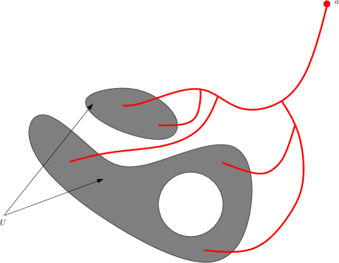
Figure 9. A parametrized path

Given a parametrized path, $\gamma:V\rightarrow\mbox{\rm R}^{k}$, we will refer to $U=\pi_{1\ldots k}(V)$ as its base. Also, any semi-algebraic subset $U^{\prime}\subset U$ of the base of such a parametrized path, defines in a natural way the restriction of $\gamma$ to the base $U^{\prime}$, which is another parametrized path, obtained by restricting $\gamma$ to the set $V^{\prime}\subset V$, defined by $V^{\prime}=\{(x,t)\mid x\in U^{\prime},0\leq t\leq\ell(x)\}$.

The following proposition which appears in [20] describes a crucial property of parametrized paths, which makes them useful in algorithms for computing Betti numbers of semi-algebraic sets.

Proposition 6.2.

[20] Let $\gamma:V\rightarrow R^{k}$ be a parametrized path such that $U=\pi_{1\ldots k}(V)$ is closed and bounded. Then, the image of $\gamma$ is semi-algebraically contractible.

It is also shown in [20] that,

Theorem 6.3.

Moreover, there exists an algorithm that takes as input a finite set of polynomials ${\mathcal{P}}\subset\mbox{\rm R}[X_{1},\ldots,X_{k}]$, and produces as output,

• a finite set of polynomials ${\mathcal{A}}\subset\mbox{\rm R}[X_{1},\ldots,X_{k}]$,

• a finite set $\Theta$ of quantifier free formulas, with atoms of the form $P=0,P>0,P<0,\;P\in{\mathcal{A}}$, such that for every semi-algebraically connected component $S$ of the realization of every weak sign condition on ${\mathcal{P}}$ on ${\rm Z}(Q,\mbox{\rm R}^{k})$, there exists a subset $\Theta(S)\subset\Theta$ such that $\displaystyle{S=\bigcup_{\theta\in\Theta(S)}{\mathcal{R}}(\theta,{\rm Z}(Q,\mbox{\rm R}^{k})),}$

• for every $\theta\in\Theta$, a parametrized path

  $$\halign{\hbox to\displaywidth{$\hfil\displaystyle#\hfil$}\cr 0.0pt{\hfil$\displaystyle\gamma_{\theta}:V_{\theta}\rightarrow\mbox{\rm R}^{k},\crcr}}$$

  with base $U_{\theta}={\mathcal{R}}(\theta,{\rm Z}(Q,\mbox{\rm R}^{k}))$, such that for each $y\in{\mathcal{R}}(\theta,{\rm Z}(Q,\mbox{\rm R}^{k})),$ $\mbox{\rm Im}\;\gamma_{\theta}(y,\cdot)$ is a semi-algebraic path which connects the point $y$ to a distinguished point $a_{\theta}$ of some roadmap $\mbox{\rm RM}({\rm Z}({\mathcal{P}}^{\prime}\cup\{Q\},\mbox{\rm R}^{k}))$ where ${\mathcal{P}}^{\prime}\subset{\mathcal{P}}$, staying inside ${{\mathcal{R}}}(\overline{\sigma}(y),{\rm Z}(Q,\mbox{\rm R}^{k})).$

Moreover, the complexity of the algorithm is $s^{k^{\prime}+1}d^{O(k^{4})}$, where $s$ is a bound on the number of elements of ${\mathcal{P}}$ and $d$ is a bound on the degrees of $Q$ and the elements of ${\mathcal{P}}$.

6.1.2. Constructing Coverings of Closed Semi-algebraic Sets by Closed Contractible Sets

The parametrized paths obtained in Theorem 6.3 are not necessarily closed or even contractible, but become so after making appropriate modifications. At the same time it is possible to maintain the covering property, namely for any given ${\mathcal{P}}$-closed semi-algebraic $S$ set, there exists a set of modified parametrized paths, whose union is $S$. Moreover, these modified sets are closed and contractible. We omit the details of this (technical) construction referring the reader to [20] for more detail. Putting together the constructions outlined above we have:

Theorem 6.4.

There exists an algorithm that given as input a ${\mathcal{P}}$-closed and bounded semi-algebraic set $S$, outputs a set of formulas $\{\phi_{1},\ldots,\phi_{M}\}$ such that

• each ${\mathcal{R}}(\phi_{i},\mbox{\rm R}^{\prime k})$ is semi-algebraically contractible, and

• $\displaystyle{\bigcup_{1\leq i\leq M}{\mathcal{R}}(\phi_{i},\mbox{\rm R}^{\prime k})={\rm Ext}(S,\mbox{\rm R}^{\prime}),}$

where $\mbox{\rm R}^{\prime}$ is some real closed extension of R. The complexity of the algorithm is bounded by $s^{(k+1)^{2}}d^{O(k^{5})}$, where $s=\#{\mathcal{P}}$ and $d=\max_{P\in{\mathcal{P}}}deg(P).$

6.2. Computing the First Betti Number

It is now an easy consequence of the existence of single exponential time covering algorithm (Theorem 6.4), and Theorem 5.36 stated above, along with the fact that we can compute descriptions of the connected components of semi-algebraic sets in single exponential time, that we can compute the first Betti number of closed and bounded semi-algebraic sets in single exponential time (see Remark 5.37 above), since the dimensions of the images and kernels of the homomorphisms of the complex, ${\rm L}^{\bullet}_{2}({\mathcal{C}}(S))$ in Theorem 5.36, can then be computed using traditional algorithms from linear algebra. As mentioned earlier, for arbitrary semi-algebraic sets (not necessarily closed and bounded), there is a single exponential time reduction to the closed and bounded case using the construction of Gabrielov and Vorobjov [20, 40].

6.3. Computing the Higher Betti Numbers

6.3.1. Double Complexes Associated to Certain Covers

We now describe how covers by contractible sets of a closed and bounded semi-algebraic set, $S$, can be used for computing the higher (than the first) Betti numbers of $S$. Recall (Remark 5.39) that it is no longer possible to use the nerve complex of a (possibly non-Leray) cover by contractible sets for this purpose.

In this section, we consider a fixed family of polynomials, ${\mathcal{P}}\subset\mbox{\rm R}[X_{1},\ldots,X_{k}],$ as well as a fixed ${\mathcal{P}}$-closed and bounded semi-algebraic set, $S\subset\mbox{\rm R}^{k}$. We also fix a number, $\ell,0\leq\ell\leq k.$

We define below (see Definition 6.5 below) a finite set of indices, ${\mathbb{A}}_{S}$, which we call the set of admissible indices, and a map that associates to each $\alpha\in{\mathbb{A}}_{S}$ a closed and bounded semi-algebraic subset $X_{\alpha}\subset S$, which we call an admissible subset. The reason behind having the set of indices is that in the construction of our complex the same set might occur with different indices and we would like to distinguish these occurrences from each other.

To each $\alpha\in{\mathbb{A}}_{S}$, we will associate its level, denoted $\mbox{\rm level}(\alpha)$, which is an integer between $0$ and $\ell$. The set ${\mathbb{A}}_{S}$ will be partially ordered, and we denote by ${\rm an}(\alpha)\subset{\mathbb{A}}_{S}$, the set of ancestors of $\alpha$ under this partial order. For $\alpha,\beta\in{\mathbb{A}}_{S}$, $\beta\in{\rm an}(\alpha)$ will imply that $X_{\alpha}\subset X_{\beta}$.

For each admissible index $\alpha\in{\mathbb{A}}_{S}$, we define a double complex, ${\mathcal{M}}^{\bullet,\bullet}(\alpha)$, such that

(6.1) $${\rm H}^{i}({\rm Tot}^{\bullet}({\mathcal{M}}^{\bullet,\bullet}(\alpha)))\cong{\rm H}^{i}(X_{\alpha}),\;0\leq i\leq\ell-\mbox{\rm level}(\alpha),$$

and for each pair $\alpha,\beta\in{\mathbb{A}}_{S}$ with $\alpha\in{\rm an}(\beta)$ a homomorphism,

(6.2) $$r_{\alpha,\beta}^{\bullet,\bullet}:{\mathcal{M}}^{\bullet,\bullet}(\alpha)\rightarrow{\mathcal{M}}^{\bullet,\bullet}(\beta),$$

which induces the restriction homomorphisms between the cohomology groups via the isomorphisms in

$$\halign{\hbox to\displaywidth{$\hfil\displaystyle#\hfil$}\cr 0.0pt{\hfil$\displaystyle r^{*}_{\alpha,\beta}:{\rm H}^{i}(X_{\alpha})\rightarrow{\rm H}^{i}(X_{\beta})\crcr}}$$

for $0\leq i\leq\ell-\mbox{\rm level}(\alpha)$ via the isomorphisms in (6.1).

The main idea behind the construction of the double complex ${\mathcal{M}}^{\bullet,\bullet}(\alpha)$ is a recursive one. Associated to any cover of $X_{\alpha}$ there exists a double complex (the Mayer-Vietoris double complex) arising from the generalized Mayer-Vietoris exact sequence (see Section 5.6). If the individual sets of the cover of $X$ are all contractible, then the first column of the ${}^{\prime}E_{1}$-term of the corresponding spectral sequence (cf. Eqn. (5.23)) is zero except at the first row. The cohomology groups of the associated total complex of the Mayer-Vietoris double complex are isomorphic to those of $X_{\alpha}$ and thus in order to compute $b_{0}(X_{\alpha}),\ldots,b_{\ell-\mbox{\rm level}(\alpha)}(X_{\alpha}),$ it suffices to compute a suitable truncation of the Mayer-Vietoris double complex. Computing (even the truncated) Mayer-Vietoris double complex directly within a single exponential time complexity is not possible by any known method, since we are unable to compute triangulations of semi-algebraic sets in single exponential time. However, making use of the cover construction recursively, we are able to compute another double complex, ${\mathcal{M}}^{\bullet,\bullet}(\alpha)$, which has much smaller size, but whose associated spectral sequence, ${}^{\prime}E_{*}$, is isomorphic to the one corresponding to the Mayer-Vietoris double complex. Hence, by Theorem 5.43 (Comparison Theorem) ${\rm Tot}^{\bullet}({\mathcal{M}}^{\bullet,\bullet}(\alpha))$, is quasi-isomorphic to the associated total complex of the Mayer-Vietoris double complex (see Proposition 6.8 below). The construction of ${\mathcal{M}}^{\bullet,\bullet}(\alpha)$ is possible in single exponential time since the covers can be computed in single exponential time.

Finally, given any closed and bounded semi-algebraic set $X\subset\mbox{\rm R}^{k}$, we will denote by ${\mathcal{C}}^{\prime}(X)$, a fixed cover of $X$ (we will assume that the construction implicit in Theorem 6.4 provides such a cover).

We now define ${\mathbb{A}}_{S}$, and for each $\alpha\in{\mathbb{A}}_{S}$ a cover ${\mathcal{C}}(\alpha)$ of $X_{\alpha}$ obtained by enlarging the cover ${\mathcal{C}}^{\prime}(X_{\alpha})$.

Definition 6.5 (Admissible indices and covers).

${\mathbb{A}}_{S}$ is defined by induction on level.

1. Firstly, $0\in{\mathbb{A}}_{S}$, $\mbox{\rm level}(0)=0,$ $X_{0}=S$, ${\rm an}(0)=\emptyset$, and ${\mathcal{C}}(0)={\mathcal{C}}^{\prime}(S)$.

2. The admissible indices at level ${i+1}$ are now inductively defined in terms of the admissible indices at level $\leq i$.

   The set of admissible indices at level $i+1$ is

   (6.3) $$\mathop{\makebox[0.0pt]{\hskip 13.99995pt$\boldsymbol{\cdot}$}\bigcup}_{\alpha\in{\mathbb{A}}_{S},\mbox{\rm level}(\alpha)=i}\{\alpha_{0}\cdot\alpha_{1}\cdots\alpha_{j}\mid\alpha_{i}\in{\mathcal{C}}(\alpha),0\leq j\leq\ell-i+1\},$$

   where $\mathop{\makebox[0.0pt]{\hskip 13.99995pt$\boldsymbol{\cdot}$}\bigcup}$ denotes the disjoint union, and for each $\beta=\alpha_{0}\cdot\alpha_{1}\cdots\alpha_{j}$ we set $X_{\beta}=X_{\alpha_{0}}\cap\cdots\cap X_{\alpha_{j}}$.

   We now enlarge the set of ancestor relations by adding:

   1. For each $\{\alpha_{0},\ldots,\alpha_{m}\}\subset\{\beta_{0},\ldots,\beta_{n}\}\subset{\mathcal{C}}(\alpha)$, with $n\leq\ell-i+1$, $\alpha_{0}\cdots\alpha_{m}\in{\rm an}(\beta_{0}\cdots\beta_{n}),$ and $\alpha\in{\rm an}(\beta_{0}\cdots\beta_{n})$.

   2. Moreover, if $\alpha_{1}\cdots\alpha_{m},\beta_{0}\cdots\beta_{n}\in{\mathbb{A}}_{S}$ are such that for every $j\in\{0,\ldots,n\}$ there exists $i\in\{0,\ldots,m\}$ such that $\alpha_{i}$ is an ancestor of $\beta_{j}$, then $\alpha_{0}\cdots\alpha_{m}$ is an ancestor of $\beta_{0}\cdots\beta_{n}$.

   3. The ancestor relation is transitively closed, so that ancestor of an ancestor is also an ancestor.

   Finally, for each $\alpha\in{\mathbb{A}}_{S}$ at level $i+1$, we define ${\mathcal{C}}(\alpha)$ as follows. Let ${\rm an}(\alpha)=\{\alpha_{1},\ldots,\alpha_{N}\}$.

   (6.4) $${\mathcal{C}}(\alpha)=\mathop{\makebox[0.0pt]{\hskip 13.99995pt$\boldsymbol{\cdot}$}\bigcup}{\mathcal{C}}^{\prime}(\beta_{1}\cdots\beta_{N}\cdot\alpha).$$

   where the disjoint union is taken over all tuples $(\beta_{1},\ldots,\beta_{N})$ satisfying for each $1\leq i,j\leq N$, $\beta_{i}\in{\mathcal{C}}(\alpha_{i})$, and if $\alpha_{i}\in{\rm an}(\alpha_{j})$ then $\beta_{i}\in{\rm an}(\beta_{j})$.

Observe that by the above definition, if $\alpha,\beta\in{\mathbb{A}}_{S}$ and $\beta\in{\rm an}(\alpha)$, then each $\alpha^{\prime}\in{\mathcal{C}}(\alpha)$ has a unique ancestor in each ${\mathcal{C}}(\beta)$, which we will denote by $a_{\alpha,\beta}(\alpha^{\prime})$.

The mappings $a_{\alpha,\beta}$ has the property that if $\beta\in{\rm an}(\alpha)$ and $\gamma\in{\rm an}(\beta)$, then $a_{\alpha,\gamma}=a_{\beta,\gamma}\circ a_{\alpha,\beta}$.

Now, suppose that there is a procedure for computing ${\mathcal{C}}^{\prime}(X)$, for any given ${\mathcal{P}}^{\prime}$-closed and bounded semi-algebraic set, $X$, such that the number and the degrees of the polynomials appearing the descriptions of the semi-algebraic sets, $X_{\alpha},\alpha\in{\mathcal{C}}^{\prime}(X)$, is bounded by

(6.5) $$D^{k^{c_{1}}},$$

where $c_{1}>0$ is some absolute constant, and $D=\sum_{P\in{\mathcal{P}}^{\prime}}\deg(P).$

Using the above procedure for computing ${\mathcal{C}}^{\prime}(X)$, and the definition of ${\mathbb{A}}_{S}$, we have the following quantitative bounds on $\#{\mathbb{A}}_{S}$ and the semi-algebraic sets $X_{\alpha},\alpha\in{\mathbb{A}}_{S}$, which is crucial in proving the single exponential complexity bound of the algorithm for computing the first few Betti numbers of semi-algebraic sets.

Proposition 6.6.

[10] Let $S\subset\mbox{\rm R}^{k}$ be a ${\mathcal{P}}$-closed semi-algebraic set, where ${\mathcal{P}}\subset\mbox{\rm R}[X_{1},\ldots,X_{k}]$ is a family of $s$ polynomials of degree at most $d$. Then $\#A_{S}$, as well as the number of polynomials used to define the semi-algebraic sets $X_{\alpha},\alpha\in{\mathbb{A}}_{S}$ and the the degrees of these polynomials, are all bounded by $(sd)^{k^{O(\ell)}}.$

6.3.2. Double Complex Associated to a Cover

Given the different covers described above, we now associate to each $\alpha\in{\mathbb{A}}_{S}$ a double complex, ${\mathcal{M}}^{\bullet,\bullet}(\alpha),$ and for every $\beta\in{\mathbb{A}}_{S}$, such that $\alpha\in{\rm an}(\beta)$, and $\mbox{\rm level}(\alpha)=\mbox{\rm level}(\beta)$, a restriction homomorphism:

$$r_{\alpha,\beta}^{\bullet,\bullet}:{\mathcal{M}}^{\bullet,\bullet}(\alpha)\rightarrow{\mathcal{M}}^{\bullet,\bullet}(\beta),$$

satisfying the following:

1. (6.6) $${\rm H}^{i}({\rm Tot}^{\bullet}({\mathcal{M}}^{\bullet,\bullet}(\alpha)))\cong{\rm H}^{i}(X_{\alpha}),\;\mbox{\rm for}\;0\leq i\leq\ell-\mbox{\rm level}(\alpha).$$

2. The restriction homomorphism

   $$r_{\alpha,\beta}^{\bullet,\bullet}:{\mathcal{M}}^{\bullet,\bullet}(\alpha)\rightarrow{\mathcal{M}}^{\bullet,\bullet}(\beta),$$

   induces the restriction homomorphisms between the cohomology groups:

   $$\halign{\hbox to\displaywidth{$\hfil\displaystyle#\hfil$}\cr 0.0pt{\hfil$\displaystyle r^{*}_{\alpha,\beta}:{\rm H}^{i}(X_{\alpha})\rightarrow{\rm H}^{i}(X_{\beta})\crcr}}$$

   for $0\leq i\leq\ell-\mbox{\rm level}(\alpha)$ via the isomorphisms in (6.6).

We now define the double complex ${\mathcal{M}}^{\bullet,\bullet}(\alpha)$. The double complex ${\mathcal{M}}^{\bullet,\bullet}(\alpha)$ is constructed inductively using induction on $\mbox{\rm level}(\alpha)$.

Definition 6.7.

The base case is when $\mbox{\rm level}(\alpha)=\ell$. In this case the double complex, ${\mathcal{M}}^{\bullet,\bullet}(\alpha)$ is defined by:

$$\begin{array}[]{ccll}{\mathcal{M}}^{0,0}(\alpha)&=&\bigoplus_{{\alpha_{0}}\;\in\;{\mathcal{C}}(\alpha)}\;{\rm H}^{0}(X_{\alpha_{0}}),\cr{\mathcal{M}}^{1,0}(\alpha)&=&\bigoplus_{{\alpha_{0}},{\alpha_{1}}\;\in\;{\mathcal{C}}(\alpha)}\;{\rm H}^{0}(X_{\alpha_{0}\cdot\alpha_{1}}),\cr{\mathcal{M}}^{p,q}(\alpha)&=&0,\;\mbox{if}\;q>0\;\mbox{or}\;p>1.\cr\end{array}$$

This is shown diagrammatically below.

$${\tiny\begin{diagram}}$$

The only non-trivial homomorphism in the above complex,

$$\halign{\hbox to\displaywidth{$\hfil\displaystyle#\hfil$}\cr 0.0pt{\hfil$\displaystyle\delta:\bigoplus_{{\alpha_{0}}\in{\mathcal{C}}(\alpha)}{\rm H}^{0}(X_{\alpha_{0}})\longrightarrow\bigoplus_{{\alpha_{0}},{\alpha_{1}}\in{\mathcal{C}}(\alpha)}{\rm H}^{0}(X_{\alpha_{0}\cdot\alpha_{1}})\crcr}}$$

is defined as follows.

$\delta(\phi)_{\alpha_{0},\alpha_{1}}=(\phi_{\alpha_{1}}-\phi_{\alpha_{0}})|_{X_{\alpha_{0}\cdot\alpha_{1}}}$ for $\phi\in\bigoplus_{{\alpha_{0}}\in{\mathcal{C}}(\alpha)}{\rm H}^{0}(X_{\alpha_{0}}).$

For every $\beta\in{\mathbb{A}}_{S}$, such that $\alpha\in{\rm an}(\beta)$, and $\mbox{\rm level}(\alpha)=\mbox{\rm level}(\beta)=\ell$, we define $r_{\alpha,\beta}^{0,0}:{\mathcal{M}}^{0,0}(\alpha)\rightarrow{\mathcal{M}}^{0,0}(\beta)$, as follows.

Recall that, $\displaystyle{{\mathcal{M}}^{0,0}(\alpha)=\bigoplus_{\alpha_{0}\;\in\;{\mathcal{C}}(\alpha)}\;{\rm H}^{0}(X_{\alpha_{0}}),}$ and $\displaystyle{{\mathcal{M}}^{0,0}(\beta)=\bigoplus_{\beta_{0}\;\in\;{\mathcal{C}}(\beta)}\;{\rm H}^{0}(X_{\beta_{0}}).}$

For $\phi\in{\mathcal{M}}^{0,0}(\alpha)$ and $\beta_{0}\in{\mathcal{C}}(\beta)$ we define

$$\halign{\hbox to\displaywidth{$\hfil\displaystyle#\hfil$}\cr 0.0pt{\hfil$\displaystyle r_{\alpha,\beta}^{0,0}(\phi)_{\beta_{0}}=\phi_{a_{\beta,\alpha}(\beta_{0})}|_{X_{\beta_{0}}}.\crcr}}$$

We define $r_{\alpha,\beta}^{1,0}:{\mathcal{M}}^{1,0}(\alpha)\rightarrow{\mathcal{M}}^{1,0}(\beta),$ in a similar manner. More precisely, for $\phi\in{\mathcal{M}}^{0,0}(\alpha)$ and $\beta_{0},\beta_{1}\in{\mathcal{C}}(\beta)$, we define

$$\halign{\hbox to\displaywidth{$\hfil\displaystyle#\hfil$}\cr 0.0pt{\hfil$\displaystyle r_{\alpha,\beta}^{1,0}(\phi)_{\beta_{0},\beta_{1}}=\phi_{a_{\beta,\alpha}(\beta_{0})\cdot a_{\beta,\alpha}(\beta_{1})}|_{X_{\beta_{0}\cdot\beta_{1}}}.\crcr}}$$

(The inductive step) In general the ${\mathcal{M}}^{p,q}(\alpha)$ are defined as follows using induction on $\mbox{\rm level}(\alpha)$ and with $n_{\alpha}=\ell-\mbox{\rm level}(\alpha)+1.$

$$\halign{\hbox to\displaywidth{$\hfil\displaystyle#\hfil$}\cr 0.0pt{\hfil$\displaystyle\begin{array}[]{ll}{\mathcal{M}}^{0,0}(\alpha)=\bigoplus_{{\alpha_{0}}\;\in\;{\mathcal{C}}(\alpha)}\;{\rm H}^{0}(X_{\alpha_{0}}),&\cr{\mathcal{M}}^{0,q}(\alpha)=0,&0<q,\cr{\mathcal{M}}^{p,q}(\alpha)=\bigoplus_{\alpha_{0}<\cdots<\alpha_{p},\;{\alpha_{i}}\in{\mathcal{C}}(\alpha)}\;{\rm Tot}^{q}({\mathcal{M}}^{\bullet,\bullet}({\alpha_{0}\cdots\alpha_{p}})),&0<p,\;0<p+q\leq n_{\alpha},\cr{\mathcal{M}}^{p,q}(\alpha)=0,&\;\mbox{else}.\end{array}\crcr}}$$

The double complex ${\mathcal{M}}^{\bullet,\bullet}(\alpha)$ is shown in the following diagram:

$${\tiny\begin{diagram}}$$

The vertical homomorphisms, $d$, in ${\mathcal{M}}^{\bullet,\bullet}(\alpha)$ are those induced by the differentials in the various

$${\rm Tot}^{\bullet}({\mathcal{M}}^{\bullet,\bullet}({\alpha_{0}\cdots\alpha_{p}})),{\alpha_{i}}\in{\mathcal{C}}(\alpha).$$

The horizontal ones are defined by generalized restriction as follows. Let

$$\phi\in\bigoplus_{\alpha_{0}<\cdots<\alpha_{p},\alpha_{i}\in{\mathcal{C}}(\alpha)}{\rm Tot}^{q}({\mathcal{M}}^{\bullet,\bullet}({\alpha_{0}\cdots\alpha_{p}})),$$

with

$$\phi_{\alpha_{0},\ldots,\alpha_{p}}=\bigoplus_{0\leq j\leq q}\phi_{\alpha_{0},\ldots,\alpha_{p}}^{j},$$

and

$$\phi_{\alpha_{0},\ldots,\alpha_{p}}^{j}\in{\mathcal{M}}^{j,q-j}({\alpha_{0}\cdots\alpha_{p}}).$$

We define

$$\halign{\hbox to\displaywidth{$\hfil\displaystyle#\hfil$}\cr 0.0pt{\hfil$\displaystyle\delta:\bigoplus_{\alpha_{0}<\cdots<\alpha_{p},\alpha_{i}\in{\mathcal{C}}(\alpha)}{\rm Tot}^{q}({\mathcal{M}}^{\bullet,\bullet}({\alpha_{0}\cdots\alpha_{p}}))\longrightarrow\bigoplus_{\alpha_{0}<\cdots<\alpha_{p+1}}{\rm Tot}^{q}({\mathcal{M}}^{\bullet,\bullet}({\alpha_{0}\cdots\alpha_{p+1}}))\crcr}}$$

by

$$\halign{\hbox to\displaywidth{$\hfil\displaystyle#\hfil$}\cr 0.0pt{\hfil$\displaystyle\delta(\phi)_{\alpha_{0},\ldots,\alpha_{p+1}}=\bigoplus_{0\leq i\leq p+1}(-1)^{i}\bigoplus_{0\leq j\leq q}r_{{\alpha_{0}\cdots\hat{\alpha_{i}}\cdots\alpha_{p+1}},{\alpha_{0}\cdots\alpha_{p+1}}}^{j,q-j}(\phi_{\alpha_{0},\ldots,\hat{\alpha_{i}},\ldots,\alpha_{p+1}}^{j}),\crcr}}$$

noting that for each $i,0\leq i\leq p+1,$ ${\alpha_{0}\cdots\hat{\alpha_{i}}\cdots\alpha_{p+1}}$ is an ancestor of ${\alpha_{0}\cdots\alpha_{p+1}}$, and

$$\mbox{\rm level}({\alpha_{0}\cdots\hat{\alpha_{i}}\cdots\alpha_{p+1}})=\mbox{\rm level}({\alpha_{0}\cdots\alpha_{p+1}})=\mbox{\rm level}(\alpha)+1,$$

and hence the homomorphisms $r_{{\alpha_{0}\cdots\hat{\alpha_{i}}\cdots\alpha_{p+1}},{\alpha_{0}\cdots\alpha_{p+1}}}^{j,q-j}$ are already defined by induction.

Now let, $\alpha,\beta\in{\mathbb{A}}_{S}$ with $\alpha$ an ancestor of $\beta$ and $\mbox{\rm level}(\alpha)=\mbox{\rm level}(\beta).$ We define the restriction homomorphism,

$$r_{\alpha,\beta}^{\bullet,\bullet}:{\mathcal{M}}^{\bullet,\bullet}(\alpha)\longrightarrow{\mathcal{M}}^{\bullet,\bullet}(\beta)$$

as follows.

As before, for $\phi\in{\mathcal{M}}^{0,0}(\alpha)$ and $\beta_{0}\in{\mathcal{C}}(\beta)$ we define

$$\halign{\hbox to\displaywidth{$\hfil\displaystyle#\hfil$}\cr 0.0pt{\hfil$\displaystyle r_{\alpha,\beta}^{0,0}(\phi)_{\beta_{0}}=\phi_{a_{\beta,\alpha}(\beta_{0})}|_{X_{\beta_{0}}}.\crcr}}$$

For $0<p,0<p+q\leq\ell-\mbox{\rm level}(\alpha)+1,$ we define

$$r_{\alpha,\beta}^{p,q}:{\mathcal{M}}^{p,q}(\alpha)\rightarrow{\mathcal{M}}^{p,q}(\beta),$$

as follows.

Let $\displaystyle{\phi\in{\mathcal{M}}^{p,q}(\alpha)=\bigoplus_{\alpha_{0}<\cdots<\alpha_{p},\;{\alpha_{i}}\in{\mathcal{C}}(\alpha)}\;{\rm Tot}^{q}({\mathcal{M}}^{\bullet,\bullet}({\alpha_{0}\cdots\alpha_{p}})).}$ We define

$$r_{\alpha,\beta}^{p,q}(\phi)=\bigoplus_{\beta_{0}<\cdots<\beta_{p},\beta_{i}\in{\mathcal{C}}(\beta)}\bigoplus_{0\leq i\leq q}r_{a_{\beta,\alpha}({\beta_{0}\cdots\beta_{p}}),{\beta_{0}\cdots\beta_{p}}}^{i,q-i}\phi_{a_{\beta,\alpha}({\beta_{0}}),\ldots,a_{\beta,\alpha}({\beta_{p}})}^{i},$$

where $a_{\beta,\alpha}({\beta_{0}\cdots\beta_{p}})=a_{\beta,\alpha}({\beta_{0}})\cdots a_{\beta,\alpha}({\beta_{p}}).$ Moreover,

$$\mbox{\rm level}(a_{\beta,\alpha}({\beta_{0}\cdots\beta_{p}}))=\mbox{\rm level}({\beta_{0}\cdots\beta_{p}})=\mbox{\rm level}(\alpha)+1,$$

and hence we can assume that the homomorphisms $r_{a_{\beta,\alpha}({\beta_{0}\cdots\beta_{p}}),{\beta_{0}\cdots\beta_{p}}}^{\bullet,\bullet}$ used in the definition of $r_{\alpha,\beta}^{\bullet,\bullet}$ are already defined by induction.

The following proposition proved in [10] is the key ingredients in the single exponential time algorithm for computing the first few Betti numbers of semi-algebraic sets.

Proposition 6.8.

[10] For each $\alpha\in{\mathbb{A}}_{S}$ the double complex ${\mathcal{M}}^{\bullet,\bullet}(\alpha)$ satisfies the following properties:

1. ${\rm H}^{i}({\rm Tot}^{\bullet}({\mathcal{M}}^{\bullet,\bullet}(\alpha)))\cong{\rm H}^{i}(X_{\alpha})$ for $0\leq i\leq\ell-\mbox{\rm level}(\alpha)$.

2. For every $\beta\in{\mathbb{A}}_{S}$, such that $\alpha$ is an ancestor of $\beta$, and $\mbox{\rm level}(\alpha)=\mbox{\rm level}(\beta)$, the homomorphism, $r_{\alpha,\beta}^{\bullet,\bullet}:{\mathcal{M}}^{\bullet,\bullet}(\alpha)\rightarrow{\mathcal{M}}^{\bullet,\bullet}(\beta),$ induces the restriction homomorphisms between the cohomology groups:

   $$\halign{\hbox to\displaywidth{$\hfil\displaystyle#\hfil$}\cr 0.0pt{\hfil$\displaystyle r^{*}:{\rm H}^{i}(X_{\alpha})\longrightarrow{\rm H}^{i}(X_{\beta})\crcr}}$$

   for $0\leq i\leq\ell-\mbox{\rm level}(\alpha)$ via the isomorphisms in (1).

Proof Sketch.

For the benefit of the reader we include an outline of the proof of Proposition 6.8 referring the reader to [10] for more detail. The proof is by induction on ${\rm level}(\alpha)$. After having chosen a suitably fine triangulation $\Delta$ of $S$ which respects all the admissible subsets $X_{\alpha}$, we construct by induction on ${\rm level}(\alpha)$, for each $\alpha\in{\mathbb{A}}_{S}$, a double complex $\mbox{\rm D}^{\bullet,\bullet}(\alpha)$ and homomorphisms

$$\phi^{\bullet,\bullet}:{\mathcal{M}}^{\bullet,\bullet}(\alpha)\rightarrow\mbox{\rm D}^{\bullet,\bullet}(\alpha),$$

and

$$\psi^{\bullet}:\mbox{\rm C}^{\bullet}(\Delta_{\alpha})\rightarrow{\rm Tot}^{\bullet}(\mbox{\rm D}^{\bullet,\bullet}(\alpha)),$$

where $\Delta_{\alpha}$ denotes the restriction of the triangulation $\Delta$ to $X_{\alpha}$. It is then shown (inductively) that each homomorphism in the following diagram is a quasi-isomorphism.

(6.7) $$\begin{diagram}$$

This suffices to prove the proposition. ∎

We now give an example of the construction of the complex described above in a very simple situation.

Example 6.9.

We take for the set $S$, the unit sphere $\mbox{${\bf S}$}^{2}\subset\mbox{\rm R}^{3}$. Even though this example looks very simple, it is actually illustrative of the main topological ideas behind the construction of the complex ${\mathcal{M}}^{\bullet,\bullet}(S)$ starting from a cover of $S$ by two closed hemispheres meeting at the equator. Since the intersection of the two hemisphere is a topological circle which is not contractible, Theorem 5.34 is not applicable. Using Theorem 5.36 we can compute ${\rm H}^{0}(S),{\rm H}^{1}(S)$, but it is not enough to compute ${\rm H}^{2}(S)$. The recursive construction of ${\mathcal{M}}^{\bullet,\bullet}$ described in the last section overcomes this problem and this is illustrated in the example.

Figure 10. Example of $\mbox{${\bf S}$}^{2}\subset\mbox{\rm R}^{3}$

We first fix some notation (see Figure 10). Let $H_{1}$ and $H_{2}$ denote the closed upper and lower hemispheres respectively. Let $H_{12}=H_{1}\cap H_{2}$ denote the equator, and let $H_{12}=C_{1}\cup C_{2}$, where $C_{1},C_{2}$ are closed semi-circular arcs. Finally, let $C_{12}=C_{1}\cap C_{2}=\{P_{1},P_{2}\}$, where $P_{1},P_{2}$ are two antipodal points.

For the purpose of this example, we will take for the covers ${\mathcal{C}^{\prime}}$ the obvious ones, namely:

$$\begin{array}[]{cccc}{\mathcal{C}}^{\prime}(S)&=&\{H_{1},H_{2}\},&\\ {\mathcal{C}}^{\prime}(H_{i})&=&\{H_{i}\},&i=1,2,\\ {\mathcal{C}}^{\prime}(H_{12})&=&\{C_{1},C_{2}\},&\\ {\mathcal{C}}^{\prime}(C_{i})&=&\{C_{i}\},&i=1,2,\\ {\mathcal{C}}^{\prime}(C_{12})&=&\{P_{1},P_{2}\},\\ {\mathcal{C}}^{\prime}(P_{i})&=&\{P_{i}\},&i=1,2.\\ \end{array}$$

Note that, in order not to complicate notation further, we are using the same names for the elements of ${\mathcal{C}}^{\prime}(\cdot)$, as well as their associated sets. Strictly speaking, we should have defined,

$${\mathcal{C}}^{\prime}(S)=\{\alpha_{1},\alpha_{2}\},\;X_{\alpha_{1}}=H_{1},X_{\alpha_{2}}=H_{2},\ldots.$$

However, since each set occurs at most once, this does not create confusion in this example.

Note that the elements of the sets occurring on the right are all closed, bounded contractible subsets of $S$. It is now easy to check from Definition 6.5, that the elements of ${\mathbb{A}}_{S}$ in order of their levels as follows.

1. Level $0$:

   $$0\in{\mathbb{A}}_{S},\mbox{\rm level}(0)=0,$$

   and

   $$\begin{array}[]{cccc}{\mathcal{C}}(0)&=&\{\alpha_{1},\alpha_{2}\},&X_{\alpha_{1}}=H_{1},X_{\alpha_{2}}=H_{2}.\\ \end{array}$$

2. Level $1$: The elements of level $1$ are

   $$\alpha_{1},\alpha_{2},\alpha_{1}\cdot\alpha_{2},$$

   and

   $$\begin{array}[]{cccc}{\mathcal{C}}(\alpha_{1})&=&\{\beta_{1}\},&X_{\beta_{1}}=H_{1},\\ {\mathcal{C}}(\alpha_{2})&=&\{\beta_{2}\},&X_{\beta_{2}}=H_{2},\\ {\mathcal{C}}(\alpha_{1}\cdot\alpha_{2})&=&\{\beta_{3},\beta_{4}\},&X_{\beta_{3}}=C_{1},X_{\beta_{4}}=C_{2}.\\ \end{array}$$

3. Level $2$: The elements of level $2$ are $\beta_{1},\beta_{2},\beta_{3},\beta_{4},\beta_{3}\cdot\beta_{4}$. We also have,

   $$\begin{array}[]{ccccc}{\mathcal{C}}(\beta_{i})&=&\{\gamma_{i}\},&X_{\gamma_{i}}=H_{i},&i=1,2,\\ {\mathcal{C}}(\beta_{i})&=&\{\gamma_{i}\},&X_{\gamma_{i}}=C_{i-2},&i=3,4,\\ {\mathcal{C}}(\beta_{3}\cdot\beta_{4})&=&\{\gamma_{5},\gamma_{6}\},&X_{\gamma_{i}}=P_{i-4},&i=5,6.\\ \end{array}$$

We now display diagrammatically the various complexes, ${\mathcal{M}}^{\bullet,\bullet}(\alpha)$ for $\alpha\in{\mathbb{A}}_{S}$ starting at level $2$.

1. Level $2$: For $1\leq i\leq 4$, we have

   $${\mathcal{M}}^{\bullet,\bullet}(\beta_{i}) =$$

   Notice that for $1\leq i\leq 4$,

   $${\rm H}^{0}({\rm Tot}^{\bullet}({\mathcal{M}}^{\bullet,\bullet}(\beta_{i})))\cong{\rm H}^{0}(X_{\beta_{i}})\cong{\mathbb{Q}}.$$

   The complex ${\mathcal{M}}^{\bullet,\bullet}(\beta_{3}\cdot\beta_{4})$ is shown below.

   $$\begin{diagram}$$

   Notice that,

   $${\rm H}^{0}({\rm Tot}^{\bullet}({\mathcal{M}}^{\bullet,\bullet}(\beta_{3}\cdot\beta_{4})))\cong{\rm H}^{0}(X_{\beta_{3}\cdot\beta_{4}})\cong{\mathbb{Q}}\oplus{\mathbb{Q}}.$$

2. Level $1$: For $i=1,2$, the complex ${\mathcal{M}}^{\bullet,\bullet}(\alpha_{i})$ is as follows.

   $$\begin{diagram}$$

   Notice that for $i=1,2$ and $j=0,1$,

   $${\rm H}^{j}({\rm Tot}^{\bullet}({\mathcal{M}}^{\bullet,\bullet}(\alpha_{i})))\cong{\rm H}^{j}(H_{i}).$$

   The complex ${\mathcal{M}}^{\bullet,\bullet}(\alpha_{1}\cdot\alpha_{2})$is shown below.

   $$\begin{diagram}$$

   Notice that for $j=0,1$,

   $${\rm H}^{j}({\rm Tot}^{\bullet}({\mathcal{M}}^{\bullet,\bullet}(\alpha_{1}\cdot\alpha_{2})))\cong{\rm H}^{j}(H_{12}).$$

3. Level $0$:

   The complex ${\mathcal{M}}^{\bullet,\bullet}(0)$ is shown below:

   $$\begin{diagram}$$

   The matrices for the homomorphisms, $\delta^{0,0}$ and $d^{1,0}$ in the obvious bases are both equal to

   $$\left(\begin{array}[]{cc}1&\;\;1\\ 1&\;\;1\end{array}\right).$$

   From the fact that the rank of the above matrix is $1$, it is not too difficult to deduce that, ${\rm H}^{j}({\rm Tot}^{\bullet}({\mathcal{M}}^{\bullet,\bullet}(0)))\cong{\rm H}^{j}(S)$, for $j=0,1,2$, that is

   $$\begin{array}[]{ccc}{\rm H}^{0}({\rm Tot}^{\bullet}({\mathcal{M}}^{\bullet,\bullet}(0)))&\cong&{\mathbb{Q}},\cr{\rm H}^{1}({\rm Tot}^{\bullet}({\mathcal{M}}^{\bullet,\bullet}(0)))&\cong&0,\cr{\rm H}^{2}({\rm Tot}^{\bullet}({\mathcal{M}}^{\bullet,\bullet}(0)))&\cong&{\mathbb{Q}}.\end{array}$$

6.3.3. Algorithm for Computing the First Few Betti Numbers

Using the construction of the double complex outline in Section 6.3.2, as well as the single exponential time algorithm for obtaining covers by contractible sets described in Section 6.1.2, along with straightforward algorithms from linear algebra, it is now easy to obtain the following result:

Theorem 6.10.

[10] For any given $\ell$, there is an algorithm that takes as input a ${\mathcal{P}}$-formula describing a semi-algebraic set $S\subset\mbox{\rm R}^{k}$, and outputs $b_{0}(S),\ldots,b_{\ell}(S).$ The complexity of the algorithm is $(sd)^{k^{O(\ell)}}$, where $s=\#({\mathcal{P}})$ and $d=\max_{P\in{\mathcal{P}}}{\rm deg}(P).$

Note that the complexity is single exponential in $k$ for every fixed $\ell$.

7. The Quadratic Case

7.1. Brief Outline

We denote by $\mbox{${\bf S}$}^{k}\subset\mbox{\rm R}^{k+1}$ the unit sphere centered at the origin. Consider the case of semi-algebraic subsets of the unit sphere, $\mbox{${\bf S}$}^{k}\subset\mbox{\rm R}^{k+1},$ defined by homogeneous quadratic inequalities. There is a straightforward reduction of the general problem to this special case.

Let $S\subset\mbox{${\bf S}$}^{k}$ be the set defined on $\mbox{${\bf S}$}^{k}$ by $s$ inequalities, $P_{1}\leq 0,\ldots,P_{s}\leq 0$, where $P_{1},\ldots,P_{s}\in\mbox{\rm R}[X_{0},\ldots,X_{k}]$ are homogeneous quadratic polynomials. For each $i,1\leq i\leq s$, let $S_{i}\subset\mbox{${\bf S}$}^{k}$ denote the set defined on $\mbox{${\bf S}$}^{k}$ by $P_{i}\leq 0$. Then, $\displaystyle{S=\bigcap_{i=1}^{s}S_{i}.}$ There are two main ingredients in the polynomial time algorithm for computing the top Betti numbers of $S$.

The first main idea is to consider $S$ as the intersection of the various $S_{i}$’s and to utilize the double complex arising from the generalized Mayer-Vietoris exact sequence (see Section 5). It follows from the exactness of the generalized Mayer-Vietoris sequence (see Definition 5.44), that the top dimensional cohomology groups of $S$ are isomorphic to those of the total complex associated to a suitable truncation of the Mayer-Vietoris double complex. However, computing even the truncation of the Mayer-Vietoris double complex, starting from a triangulation of $S$ would entail a doubly exponential complexity. However, we utilize the fact that terms appearing in the truncated complex depend on the unions of the $S_{i}$’s taken at most $\ell+2$ at a time (cf. Remark 5.50). There are at most $\displaystyle{\sum_{j=1}^{\ell+2}{s\choose j}}$ such sets. Moreover, for semi-algebraic sets defined by the disjunction of a small number of quadratic inequalities, we are able to compute in polynomial (in $k$) time a complex, whose homology groups are isomorphic to those of the given sets. The construction of these complexes in polynomial time is the second important ingredient in our algorithm and is outlined below in Section 7.4. These complexes along with the homomorphisms between them define another double complex whose associated spectral sequence (corresponding to the column-wise filtration) is isomorphic from the $E_{2}$ term onwards to the corresponding one of the (truncated) Mayer-Vietoris double complex (see Theorem 7.21 below). Since, we know that the latter converges to the homology groups of $S$, the top Betti numbers of $S$ are equal to the ranks of the homology groups of the associated total complex of the double complex we computed. These can then be computed using well known efficient algorithms from linear algebra.

In order to carry through the program described above we need to understand a few things about the topology of sets defined by homogeneous quadratic inequalities.

7.2. Topology of Sets Defined by Quadratic Inequalities

In this section we state a few results concerning the topology of sets defined by quadratic inequalities, which are exploited in designing efficient algorithms for computing their Betti numbers.

7.2.1. Case of One Quadratic Form

We first consider the case of a single quadratic form $Q\in\mbox{\rm R}[X_{0},\ldots,X_{k}]$. Let $S\subset\mbox{${\bf S}$}^{k}$ be the set defined by $Q\geq 0$ on the unit sphere in $\mbox{\rm R}^{k+1}$. The crucial fact that distinguishes quadratic forms from forms of higher degree is that the homotopy type of the set $S$ is determined by a single invariant attached to the quadratic form $Q$, namely its index.

Definition 7.1 (Index of a quadratic form).

For any quadratic form $Q$, ${\rm index}(Q)$ is the number of negative eigenvalues of the symmetric matrix of the corresponding bilinear form, that is of the matrix $M$ such that, $Q(x)=\langle Mx,x\rangle$ for all $x\in\mbox{\rm R}^{k+1}$ (here $\langle\cdot,\cdot\rangle$ denotes the usual inner product). We will also denote by $\lambda_{i}(Q),0\leq i\leq k$, the eigenvalues of $M$, in non-decreasing order, i.e.

$$\lambda_{0}(Q)\leq\lambda_{1}(Q)\leq\cdots\leq\lambda_{k}(Q).$$

A simple argument involving diagonalizing the quadratic form $Q$ (see [2] or [11]) yields that the homotopy type of the set $S$ defined above is related to the ${\rm index}(Q)$ by

Proposition 7.2.

The set $S$ is homotopy equivalent to the $\mbox{${\bf S}$}^{k-{\rm index}(Q)}$.

Example 7.3.

The following figure (Figure 11) illustrates Proposition 7.2. We display (from left to right) the subsets of $\mbox{${\bf S}$}^{2}$ described by the inequalities

$$X_{0}^{2}+2X_{1}^{2}+3X_{2}^{2} \geq 0\;\;({\rm index}=0),$$

$$X_{0}^{2}+2X_{1}^{2}-3X_{2}^{2} \geq 0\;\;({\rm index}=1),$$

$$X_{0}^{2}-2X_{1}^{2}-3X_{2}^{2} \geq 0\;\;({\rm index}=2)$$

respectively. Notice that each of the quadratic forms defining these sets are already in a diagonal form, and hence its index can be read off directly from the signs of the coefficients (the index is the number of negative coefficients). By Proposition 7.2 these sets have the homotopy types of $\mbox{${\bf S}$}^{2}$, $\mbox{${\bf S}$}^{1}$, and $\mbox{${\bf S}$}^{0}$ respectively, as can be also seen from the displayed images below.

Figure 11. Subsets of $\mbox{${\bf S}$}^{2}$ defined by one homogeneous quadratic inequality of index $0$, $1$ and $2$.

7.2.2. Case of Several Quadratic Forms

Now let $Q_{1},\ldots,Q_{s}$ be homogeneous quadratic polynomials in $\mbox{\rm R}[X_{0},\ldots,X_{k}]$.

We denote by $Q=(Q_{1},\ldots,Q_{s}):\mbox{\rm R}^{k+1}\rightarrow\mbox{\rm R}^{s}$, the map defined by the forms $Q_{1},\ldots,Q_{s}$.

Let

(7.1) $$T=\bigcup_{1\leq i\leq s}\{x\in\mbox{${\bf S}$}^{k}\mid Q_{i}(x)\leq 0\},$$

and let

(7.2) $$\Omega=\{\omega\in\mbox{\rm R}^{s}\mid|\omega|=1,\omega_{i}\leq 0,1\leq i\leq s\}.$$

For $\omega\in\Omega$ we denote by ${\omega}Q$ the quadratic form

(7.3) $${\omega}Q=\sum_{i=1}^{s}\omega_{i}Q_{i}.$$

Let $B\subset\Omega\times\mbox{${\bf S}$}^{k}$ be the set defined by

(7.4) $$B=\{(\omega,x)\mid\omega\in\Omega,x\in\mbox{${\bf S}$}^{k}\;\mbox{and}\;{\omega}Q(x)\geq 0\}.$$

We denote by $\phi_{1}:B\rightarrow\Omega$ and $\phi_{2}:B\rightarrow\mbox{${\bf S}$}^{k}$ the two projection maps.

$$\begin{diagram}$$

With the notation developed above we have

Proposition 7.4.

[2] The map $\phi_{2}$ gives a homotopy equivalence between $B$ and $\phi_{2}(B)=T$.

We denote by

(7.5) $$\Omega_{j}=\{\omega\in\Omega\;\mid\;\lambda_{j}({\omega}P)\geq 0\}.$$

It is clear that the $\Omega_{j}$’s induce a filtration of the space $\Omega$, i.e., $\Omega_{0}\subset\Omega_{1}\subset\cdots\subset\Omega_{k}.$

The following lemma follows directly from Proposition 7.2. It is an important ingredient in the algorithms for computing the Euler-Poincaré characteristic as well as the Betti numbers of semi-algebraic sets defined by quadratic inequalities described later.

Lemma 7.5.

The fiber of the map $\phi_{1}$ over a point $\omega\in\Omega_{j}\setminus\Omega_{j-1}$ has the homotopy type of a sphere of dimension $k-j$.

We illustrate Lemma 7.5 with an example.

Example 7.6.

In this example $s=2,k=2$, and

$$Q_{1}= -X_{0}^{2}-X_{1}^{2}-X_{2}^{2},$$

$$Q_{2}= X_{0}^{2}+2X_{1}^{2}+3X_{2}^{2}.$$

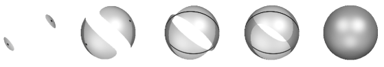
Figure 12. Type change: $\emptyset\to\mbox{${\bf S}$}^{0}\to\mbox{${\bf S}$}^{1}\to\mbox{${\bf S}$}^{2}$. $\emptyset$ is not shown.

The set $\Omega$ is the part of the unit circle in the third quadrant of the plane. In the following Figure 12, we display the fibers of the map $\varphi_{1}^{-1}(\omega)\subset B$ for a sequence of values of $\omega$ starting from $(-1,0)$ and ending at $(0,-1)$. We also show the spheres of dimensions $0,1$, and $2$, that these fibers retract to. At $\omega=(-1,0)$, it is easy to verify that ${\rm index}(\omega Q)=3$, and the fiber $\varphi_{1}^{-1}(\omega)\subset B$ is empty. Starting from $\omega=(-\cos(\arctan(1)),-\sin(\arctan(1)))$ we have ${\rm index}(\omega Q)=2$ and the fiber $\varphi_{1}^{-1}(\omega)$ consists of the union of two spherical caps homotopy equivalent to $\mbox{${\bf S}$}^{0}$. Starting from $\omega=(-\cos(\arctan(1/2)),-\sin(\arctan(1/2)))$ we have ${\rm index}(\omega Q)=1$, and the fiber $\varphi_{1}^{-1}(\omega)$ is homotopy equivalent to $\mbox{${\bf S}$}^{1}$. Finally, starting from $\omega=(-\cos(\arctan(1/3)),-\sin(\arctan(1/3)))$, ${\rm index}(\omega Q)=0$, and the fiber $\varphi_{1}^{-1}(\omega)$ stays equal to to $\mbox{${\bf S}$}^{2}$.

As a consequence of Lemma 7.5 we obtain the following proposition which relates the Euler-Poincaré characteristic of the set $T$ (cf. Eqn. (7.1)) with the Borel-Moore Euler-Poincaré characteristic (cf. Definition 5.22) of $\Omega_{j}\setminus\Omega_{j-1},\;0\leq j\leq k+1$.

Proposition 7.7.

(7.6) $$\chi(T)=\chi^{BM}(T)=\sum_{j=0}^{k+1}\chi^{BM}(\Omega_{j}\setminus\Omega_{j-1})(1+(-1)^{(k-j)}).$$

It is instructive to continue Example 7.6 and compute the Euler-Poincaré characteristic of the set $T$ in that case using Proposition 7.7.

Example 7.8.

In this example for each $0<j\leq 3$,

$$\Omega_{j}\setminus\Omega_{j-1}\mbox{ is homeomorphic to }[0,1)$$

and for $j=0$ we have

$$\Omega_{0}\setminus\Omega_{-1}=\Omega_{0}\mbox{ is homeomorphic to }[0,1].$$

Recall from Eqn. (5.8) that $\chi^{BM}([0,1))=0$ and $\chi^{BM}([0,1])=\chi([0,1])=1$. Finally using Eqn. (7.6) we deduce that

$$\chi(T)=2.$$

7.3. Computing the Euler-Poincaré Characteristics of Sets Defined by Few Quadratic Inequalities

Proposition 7.7 reduces the problem of computing the Euler-Poincaré characteristic of the set $T$, which is defined by quadratic forms in $k+1$ variables, to computing the Borel-Moore Euler-Poincaré characteristics of the sets $\Omega_{j}\setminus\Omega_{j-1}\subset\Omega$, which are defined by $O(k)$ polynomials in $s$ variables of degree also bounded by $O(k)$. We now utilize an efficient algorithm for listing the Borel-Moore Euler-Poincaré characteristics of the realizations of all all sign conditions of a family of polynomials developed in [18] to compute the terms occurring on the right hand side of Eqn. (7.6). The complexity of this algorithm is exponential in the number of variables (which is $O(s)$ in this case) and polynomial in the number and degrees of the input polynomials (which are $O(k)$ in this case).

The set $T$ is defined by a disjunction of homogeneous quadratic inequalities. But since the Euler-Poincaré characteristic satisfies the inclusion-exclusion formula (cf. Proposition 5.25), we are able to compute it for sets defined by a conjunction of such inequalities within the same asymptotic time bound by making at most $2^{s}$ calls to the algorithm for disjunctions.

For inhomogeneous quadratic inequalities there is an easy reduction to the homogeneous case (see [9] for detail). As a result we obtain

Theorem 7.9.

[9] There exists an algorithm which takes as input a closed semi-algebraic set $S\subset\mbox{\rm R}^{k}$ defined by

$$P_{1}\leq 0,\ldots,P_{s}\leq 0,P_{i}\in\mbox{\rm R}[X_{1},\ldots,X_{k}],\deg(P_{i})\leq 2,$$

and computes the Euler-Poincaré characteristic of $S$. The complexity of the algorithm is $k^{O(s)}$.

Remark 7.10.

Very recently [14] the above algorithm has been generalized to the following setting. Let

$${\mathcal{Q}}=\{Q_{1},\ldots,Q_{s}\}\subset\mbox{\rm R}[X_{1},\ldots,X_{k},Y_{1},\ldots,Y_{\ell}]$$

with $\deg_{X}(Q_{i})\leq 2,\deg_{Y}(Q_{i})\leq d,1\leq i\leq s,$ and

$${\mathcal{P}}\subset\mbox{\rm R}[Y_{1},\ldots,Y_{\ell}]$$

with $\deg(P)\leq d,P\in{\mathcal{P}}$ and $\#{\mathcal{P}}=m$. Let $S\subset\mbox{\rm R}^{k+\ell}$ be a ${\mathcal{P}}\cup{\mathcal{Q}}$-closed semi-algebraic set. Then,

Theorem 7.11.

[14] There exists an algorithm for computing the Euler-Poincaré characteristic of $S$ whose complexity is bounded by $(k\ell md)^{O(s(s+\ell))}$.

Notice that Theorem 7.11 is a generalization of Theorem 7.9 in several respects. It allows a subset of the variables to occur with degrees bigger than $2$ (and the complexity of the algorithm is exponential in the number of these variables) and it takes as input general ${\mathcal{P}}\cup{\mathcal{Q}}$-closed semi-algebraic sets, not just basic closed ones.

7.4. Computing the Betti Numbers

7.4.1. The Homogeneous Case

We first consider the homogeneous case.

Let ${\mathcal{P}}=(P_{1},\ldots,P_{s})\subset\mbox{\rm R}[X_{0},\ldots,X_{k}]$ be a $s$-tuple of quadratic forms (i.e. homogeneous quadratic polynomials). For any subset ${\mathcal{Q}}\subset{\mathcal{P}}$ we denote by $T_{\mathcal{Q}}\subset\mbox{${\bf S}$}^{k}$ the semi-algebraic set

$$\halign{\hbox to\displaywidth{$\hfil\displaystyle#\hfil$}\cr 0.0pt{\hfil$\displaystyle T_{\mathcal{Q}}=\bigcup_{P\in{\mathcal{Q}}}\{x\in\mbox{${\bf S}$}^{k}\;\mid\;P(x)\leq 0\},\crcr}}$$

and let

$$\halign{\hbox to\displaywidth{$\hfil\displaystyle#\hfil$}\cr 0.0pt{\hfil$\displaystyle S=\bigcap_{P\in{\mathcal{P}}}\{x\in\mbox{${\bf S}$}^{k}\;\mid\;P(x)\leq 0\}.\crcr}}$$

We denote by ${\rm C}^{\bullet}({\mathcal{H}}(T_{\mathcal{Q}}))$ the co-chain complex of a triangulation ${\mathcal{H}}(T_{\mathcal{Q}})$ of $T_{\mathcal{Q}}$ which is to be chosen sufficiently fine.

We first describe for each subset ${\mathcal{Q}}\subset{\mathcal{P}}$ with $\#{\mathcal{Q}}=\ell<k$ a complex, ${\mathcal{M}}^{\bullet}_{\mathcal{Q}}$, and natural homomorphisms

$$\psi_{\mathcal{Q}}:{\rm C}^{\bullet}({\mathcal{H}}(T_{\mathcal{Q}}))\rightarrow{\mathcal{M}}^{\bullet}_{\mathcal{Q}}$$

which induce isomorphisms

$$\psi_{\mathcal{Q}}^{*}:H^{*}({\rm C}^{\bullet}({\mathcal{H}}(T_{\mathcal{Q}})))\rightarrow H^{*}({\mathcal{M}}_{\mathcal{Q}}^{\bullet}).$$

Moreover, for ${\mathcal{B}}\subset{\mathcal{A}}\subset{\mathcal{P}}$ with $\#{\mathcal{A}}=\#{\mathcal{B}}+1<k$, we construct a homomorphism of complexes

$$\phi_{{\mathcal{A}},{\mathcal{B}}}:{\mathcal{M}}^{\bullet}_{\mathcal{A}}\rightarrow{\mathcal{M}}^{\bullet}_{\mathcal{B}}$$

such that the following diagram commutes.

(7.7) $$\begin{diagram}$$

In the above diagram $\phi_{{\mathcal{A}},{\mathcal{B}}}^{*}$ and $r^{*}$ are the induced homomorphisms of $\phi_{{\mathcal{A}},{\mathcal{B}}}$ and the restriction homomorphism $r$ respectively.

Now consider a fixed subset ${\mathcal{Q}}\subset{\mathcal{P}}$, which without loss of generality, we take to be $\{P_{1},\ldots,P_{\ell}\}$. Let

$$P=(P_{1},\ldots,P_{\ell}):\mbox{\rm R}^{k+1}\rightarrow\mbox{\rm R}^{\ell}$$

denote the corresponding quadratic map.

Let $\mbox{\rm R}^{\mathcal{Q}}=\mbox{\rm R}^{\ell}$ and

$$\Omega_{\mathcal{Q}}=\{\omega\in\mbox{\rm R}^{\ell}\mid|\omega|=1,\omega_{i}\leq 0,1\leq i\leq\ell\}.$$

Let $B_{\mathcal{Q}}\subset\Omega_{\mathcal{Q}}\times\mbox{${\bf S}$}^{k}$ be the set defined by

$$B_{\mathcal{Q}}=\{(\omega,x)\mid\omega\in\Omega_{\mathcal{Q}},x\in\mbox{${\bf S}$}^{k}\;\mbox{and}\;{\omega}P(x)\geq 0\},$$

and we denote by $\phi_{1,{\mathcal{Q}}}:{B}_{\mathcal{Q}}\rightarrow\Omega_{\mathcal{Q}}$ and $\phi_{2,{\mathcal{Q}}}:{B}_{\mathcal{Q}}\rightarrow\mbox{${\bf S}$}^{k}$ the two projection maps.

For each subset ${\mathcal{Q}}^{\prime}\subset{\mathcal{Q}}$ we have a natural inclusion $\Omega_{{\mathcal{Q}}^{\prime}}\hookrightarrow\Omega_{\mathcal{Q}}$.

7.4.2. Index Invariant Triangulations

We now define a certain special kind of semi-algebraic triangulation of $\Omega_{{\mathcal{Q}}}$ that will play an important role in our algorithm.

Definition 7.12 (Index Invariant Triangulation).

An index invariant triangulation of $\Omega_{{\mathcal{Q}}}$ consists of:

1. A semi-algebraic triangulation,

   $$h:\Delta_{{\mathcal{Q}}}\rightarrow\Omega_{{\mathcal{Q}}}$$

   of $\Omega_{{\mathcal{Q}}}$ which is compatible with the subsets $\Omega_{{\mathcal{Q}}^{\prime}}$ for every ${\mathcal{Q}}^{\prime}\subset{\mathcal{Q}}$ and such that for any simplex $\sigma$ of $\Delta_{{\mathcal{Q}}}$, ${\rm index}(\omega P_{\mathcal{Q}})$ as well as the multiplicities of the eigenvalues of $\omega P_{\mathcal{Q}}$ stay invariant as $\omega$ varies over $h(\sigma)$;

2. for every simplex $\sigma$ of $\Delta_{{\mathcal{Q}}}$ with ${\rm index}(\omega P_{\mathcal{Q}})=j$ for $\omega\in h(\sigma)$, a uniform description of a family of orthonormal vectors $e_{0}(\sigma,\omega),\ldots,e_{k}(\sigma,\omega)$, parametrized by $(\omega,x)\in h(\sigma)$ having the property that

   $$\{e_{j}(\sigma,\omega),\ldots,e_{k}(\sigma,\omega)\}$$

   is a basis for the linear subspace $L^{+}(\omega)\subset\mbox{\rm R}^{k+1}$ (which is the orthogonal complement to the sum of the eigenspaces corresponding to the first $j$ eigenvalues of $\omega P_{\mathcal{Q}}$).

An algorithm to compute index invariant triangulations is described in [11] (see also [14]) the complexity of this algorithm is bounded by $k^{2^{O(s)}}$. The same bound holds for the size of the complex $\Delta_{{\mathcal{Q}}}$ as well as the degrees of the polynomials occurring in the parametrized representation of the vectors $\{e_{0}(\sigma,\omega),\ldots,e_{k}(\sigma,\omega)\}$.

Now fix an index invariant triangulation $h:\Delta_{{\mathcal{Q}}}\rightarrow\Omega_{{\mathcal{Q}}}$ satisfying the complexity estimates stated above.

We now construct a cell complex homotopy equivalent to $B_{{\mathcal{Q}}}$. It is obtained by glueing together certain regular cell complexes, ${\mathcal{K}}(\sigma)$, where $\sigma\in\Delta_{{\mathcal{Q}}}$.

Figure 13. The complex $\Delta_{{\mathcal{Q}}}$.

Figure 14. The corresponding complex ${\mathcal{C}}(\Delta_{{\mathcal{Q}}})$.

Let $1\gg{\varepsilon}_{0}\gg{\varepsilon}_{1}\gg\cdots\gg{\varepsilon}_{\ell}>0$ be infinitesimals. For $\tau\in\Delta_{{\mathcal{Q}}}$ we denote by $D_{\tau}$ the subset of $\bar{\tau}$ defined by

$$D_{\tau}=\{v\in\bar{\tau}\;\mid\;{\rm dist}(v,\theta)\geq{\varepsilon}_{\dim(\theta)}\mbox{ for all }\theta\prec\sigma\}$$

where ${\rm dist}$ refers to the ordinary Euclidean distance. Now let $\sigma\prec\tau$ be two simplices of $\Delta_{{\mathcal{Q}}}$. We denote by $D_{\sigma,\tau}$ the subset of $\bar{\tau}$ defined by

$$D_{\sigma,\tau}=\{v\in\bar{\tau}\;\mid\;{\rm dist}(v,\sigma)\leq{\varepsilon}_{\dim(\sigma)},\mbox{ and }{\rm dist}(v,\theta)\geq{\varepsilon}_{\dim(\theta)}\mbox{ for all }\theta\prec\sigma\}.$$

Note that

$$\halign{\hbox to\displaywidth{$\hfil\displaystyle#\hfil$}\cr 0.0pt{\hfil$\displaystyle|\Delta_{{\mathcal{Q}}}|=\bigcup_{\sigma\in\Delta_{\mathcal{Q}}}D_{\sigma}\cup\bigcup_{\sigma,\tau\in\Delta_{\mathcal{Q}},\sigma\prec\tau}D_{\sigma,\tau}.\crcr}}$$

Also, observe that the various $D_{\tau}$’s and $D_{\sigma,\tau}$’s are all homeomorphic to closed balls and moreover all non-empty intersections between them also have the same property.

Definition 7.13.

The union of the $D_{\tau}$’s and $D_{\sigma,\tau}$’s together with the non-empty intersections between them form a regular cell complex (cf. Definition 5.4), ${\mathcal{C}}(\Delta_{{\mathcal{Q}}})$, whose underlying topological space is $|\Delta_{{\mathcal{Q}}}|$ (see Figures 13 and 14).

We now associate to each $D_{\sigma}$ (respectively, $D_{\sigma,\tau}$) a regular cell complex, ${\mathcal{K}}(\sigma)$, (respectively, ${\mathcal{K}}(\sigma,\tau)$) homotopy equivalent to $\phi_{1}^{-1}(h(D_{\sigma}))$ (respectively, $\displaystyle{\phi_{1}^{-1}(h(D_{\sigma,\tau})).}$

For each $\sigma\in\Delta_{{\mathcal{Q}}}$ and $\omega\in h(\sigma)$ let $\{e_{0}(\sigma,\omega),\ldots,e_{k}(\sigma,\omega)\}$ be the continuously varying orthonormal basis of $\mbox{\rm R}^{k+1}$ computed previously.

The orthonormal basis

$$\{e_{0}(\sigma,\omega),\ldots,e_{k}(\sigma,\omega)\}$$

determines a complete flag of subspaces, ${\mathcal{F}}(\sigma,\omega)$, consisting of

$$F^{0}(\sigma,\omega)= ~{}0,$$

$$F^{1}(\sigma,\omega)= ~{}{\rm span}(e_{k}(\sigma,\omega)),$$

$$F^{2}(\sigma,\omega,x)= ~{}{\rm span}(e_{k}(\sigma,\omega),e_{k-1}(\sigma,\omega)),$$

$$\vdots$$

$$F^{k+1}(\sigma,\omega)= ~{}\mbox{\rm R}^{k+1}.$$

Definition 7.14.

For $0\leq j\leq k$ let $c_{j}^{+}(\sigma,\omega)$ (respectively, $c_{j}^{-}(\sigma,\omega)$) denote the $(k-j)$-dimensional cell consisting of the intersection of the $F^{k-j+1}(\sigma,\omega)$ with the unit hemisphere in $\mbox{\rm R}^{k+1}$ defined by

$$\{x\in\mbox{${\bf S}$}^{k}\;\mid\; \langle x,e_{j}(\sigma,\omega)\rangle\geq 0\}$$

$$\text{(respectively, }\quad\{x\in\mbox{${\bf S}$}^{k}\;\mid\; \langle x,e_{j}(\sigma,\omega)\rangle\leq 0\}\quad).$$

The regular cell complex ${\mathcal{K}}(\sigma)$ (as well as $\mathcal{K}(\sigma,\tau)$) is defined as follows.

For each $v\in|\Delta_{{\mathcal{Q}}}|$ and $\sigma\in\Delta_{{\mathcal{Q}}}$ let $v(\sigma)\in|\sigma|$ denote the point of $|\sigma|$ closest to $v$.

The cells of ${\mathcal{K}}(\sigma)$ are

$$\{(x,\omega)\mid x\in c_{j}^{\pm}(\sigma,\omega),\omega\in h(c)\}$$

where ${\rm index}(\omega P_{\mathcal{Q}})\leq j\leq k$ and $c\in{\mathcal{C}}(\Delta_{{\mathcal{Q}}})$ is either $D_{\sigma}$ itself or a cell contained in the boundary of $D_{\sigma}$.

Similarly, the cells of ${\mathcal{K}}(\sigma,\tau)$ are

$$\{(x,\omega)\mid x\in c_{j}^{\pm}(\sigma,h(v(\sigma))),v=h^{-1}(\omega)\in c\}$$

where ${\rm index}(\omega P_{\mathcal{Q}})\leq j\leq k$ and $c\in{\mathcal{C}}(\Delta_{{\mathcal{Q}}})$ is either $D_{\sigma,\tau}$ itself or a cell contained in the boundary of $D_{\sigma,\tau}$.

Our next step is to obtain cellular subdivisions of each non-empty intersection amongst the spaces associated to the complexes constructed above and thus obtain a regular cell complex, ${\mathcal{K}}(B_{{\mathcal{Q}}})$, whose associated space, $|{\mathcal{K}}(B_{{\mathcal{Q}}})|$, will be shown to be homotopy equivalent to $B_{{\mathcal{Q}}}$.

First notice that $|{\mathcal{K}}(\sigma^{\prime},\tau^{\prime})|$ (respectively, $|{\mathcal{K}}(\sigma)|$) has a non-empty intersection with $|{\mathcal{K}}(\sigma,\tau)|$ only if $D_{\sigma^{\prime},\tau^{\prime}}$ (respectively, $D_{\sigma^{\prime}}$) intersects $D_{\sigma,\tau}$.

Let $D$ be some non-empty intersection amongst the $D_{\sigma}$’s and $D_{\sigma,\tau}$’s, i.e. $D$ is a cell of ${\mathcal{C}}(\Delta_{{\mathcal{Q}}})$. Then, $D\subset|\tau|$ for a unique simplex $\tau\in\Delta_{{\mathcal{Q}}}$ and

$$\halign{\hbox to\displaywidth{$\hfil\displaystyle#\hfil$}\cr 0.0pt{\hfil$\displaystyle D=D_{\sigma_{1},\tau}\cap\cdots\cap D_{\sigma_{p},\tau}\cap D_{\tau}\crcr}}$$

with $\sigma_{1}\prec\sigma_{2}\prec\cdots\prec\sigma_{p}\prec\sigma_{p+1}=\tau$ and $p\leq\ell$.

For each $i,1\leq i\leq p+1$, let $\{f_{0}(\sigma_{i},v),\ldots,f_{k}(\sigma_{i},v)\}$ denote a orthonormal basis of $\mbox{\rm R}^{k+1}$ where

$$f_{j}(\sigma_{i},v)=\lim_{t\rightarrow 0}e_{j}(\sigma_{i},h(tv(\sigma_{i})+(1-t)v(\sigma_{1}))),0\leq j\leq k,$$

and let ${\mathcal{F}}(\sigma_{i},v)$ denote the corresponding flag consisting of

$$F^{0}(\sigma_{i},v)= ~{}0,$$

$$F^{1}(\sigma_{i},v)= ~{}{\rm span}(f_{k}(\sigma_{i},v)),$$

$$F^{2}(\sigma_{i},v)= ~{}{\rm span}(f_{k}(\sigma_{i},v),f_{k-1}(\sigma_{i},v)),$$

$$\vdots$$

$$F^{k+1}(\sigma_{i},v)= ~{}\mbox{\rm R}^{k+1}.$$

We thus have $p+1$ different flags

$${\mathcal{F}}(\sigma_{1},v),\ldots,{\mathcal{F}}(\sigma_{p+1},v),$$

and these give rise to $p+1$ different regular cell decompositions of $\mbox{${\bf S}$}^{k}$.

Figure 15. The cell complex ${\mathcal{K}}^{\prime}(D,v)$.

There is a unique smallest regular cell complex, ${\mathcal{K}}^{\prime}(D,v)$, that refines all these cell decompositions whose cells are the following. Let $L\subset\mbox{\rm R}^{k+1}$ be a linear subspace of dimension $j,0\leq j\leq k+1$, which is an intersection of linear subspaces $L_{1},\ldots,L_{p+1}$ where $L_{i}\in{\mathcal{F}}(\sigma_{i},v),1\leq i\leq p+1\leq\ell+1$. The elements of the flags ${\mathcal{F}}(\sigma_{1},v),\ldots,{\mathcal{F}}(\sigma_{p+1},v)$ of dimension $j+1$ partition $L$ into polyhedral cones of various dimensions. The intersections of these cones with $\mbox{${\bf S}$}^{k}$ over all such subspaces $L\subset\mbox{\rm R}^{k+1}$ are the cells of ${\mathcal{K}}^{\prime}(D,v)$. Figure 15 illustrates the refinement described above in case of two flags in $\mbox{\rm R}^{3}$. We denote by ${\mathcal{K}}(D,v)$ the sub-complex of ${\mathcal{K}}^{\prime}(D,v)$ consisting of only those cells included in $L(\sigma_{1},h(v(\sigma_{1})))\cap\mbox{${\bf S}$}^{k}$.

We now triangulate $h(D)$ using the algorithm implicit in Theorem 4.5 (Triangulation) so that the combinatorial type of the arrangement of flags

$${\mathcal{F}}(\sigma_{1},v),\ldots,{\mathcal{F}}(\sigma_{p+1},v)$$

and hence the cell decomposition ${\mathcal{K}}^{\prime}(D,v)$ stays invariant over the image, $h_{D}(\theta)$, of each simplex, $\theta$, of this triangulation. Notice that the combinatorial type of the cell decomposition ${\mathcal{K}}^{\prime}(D,v)$ is determined by the signs of the inner products ${\langle}f_{j}(\sigma_{i},v),f_{j^{\prime}}(\sigma_{i^{\prime}},v){\rangle}$ where $0\leq j,j^{\prime}\leq\ell,1\leq i,i^{\prime}\leq p+1$.

We compute a family of polynomials ${\mathcal{A}}_{D}\subset\mbox{\rm R}[Z_{1},\ldots,Z_{\ell}]$ whose signs determine the vanishing or non-vanishing of the inner products ${\langle}f_{j}(\sigma_{i},v),f_{j^{\prime}}(\sigma_{i^{\prime}},v){\rangle},0\leq j,j^{\prime}\leq k,1\leq i,i^{\prime}\leq p+1$. It is then clear that the combinatorial type of the cell decomposition ${\mathcal{K}}^{\prime}(D,v)$ will stay invariant as $\omega$ varies over each connected component of any realizable sign condition on ${\mathcal{A}}_{D}\subset\mbox{\rm R}[Z_{1},\ldots,Z_{\ell}]$.

Given the complexity bounds on the rational functions defining the orthonormal bases $\{e_{0}(\sigma,\omega),\ldots,e_{\ell}(\sigma,\omega)\}$ $\omega\in h(\sigma)$, stated above that the number and degrees of the polynomials in the family ${\mathcal{A}}_{D}$ are bounded by $k^{2^{O(s)}}$. We then use the algorithm implicit in Theorem 4.5 (Triangulation) with ${\mathcal{A}}_{D}$ as input, to obtain the required triangulation.

The closures of the sets

$$\{(x,\omega)\;\mid\;x\in c\in{\mathcal{K}}(D,h^{-1}(\omega)),\;\omega\in h(h_{D}(\theta))\}$$

form a regular cell complex which we denote by ${\mathcal{K}}(D)$.

The following proposition gives an upper bound on the size of the complex ${\mathcal{K}}(D)$. We use the notation introduced in the previous paragraph.

Proposition 7.15.

For each $\omega\in h(D)$, the number of cells in ${\mathcal{K}}(D,h^{-1}(\omega))$ is bounded by $k^{O(\ell)}$. Moreover, the number of cells in the complex ${\mathcal{K}}(D)$ is bounded by $k^{2^{O(\ell)}}$.

Note that there is a homeomorphism $i_{D,\sigma_{i}}:|{\mathcal{K}}(\sigma_{i},\tau)|\cap\phi_{1}^{-1}(h(D))\rightarrow|{\mathcal{K}}(D)|$ which takes each cell of $|{\mathcal{K}}(\sigma_{i},\tau)|\cap\phi_{1}^{-1}(h(D))$ to a union of cells in ${\mathcal{K}}(D)$. We use these homeomorphisms to glue the cell complexes ${\mathcal{K}}(\sigma_{i},\tau)$ together to form the cell complex ${\mathcal{K}}(B_{{\mathcal{Q}}})$. More precisely

Definition 7.16.

${\mathcal{K}}(B_{{\mathcal{Q}}})$ is the union of all the complexes ${\mathcal{K}}(D)$ constructed above, where we use the maps $i_{D,\sigma_{i}}$ to make the obvious identifications.

We have that

Proposition 7.17.

$|{\mathcal{K}}(B_{{\mathcal{Q}}})|$ is homotopy equivalent to $B_{{\mathcal{Q}}}$.

We also have

Proposition 7.18.

The number of cells in the cell complex ${\mathcal{K}}(B_{{\mathcal{Q}}})$ is bounded by $k^{2^{O(\ell)}}$.

Proposition 7.19.

[11] For $0\leq i\leq k-1$, the induced homomorphisms

$$\psi_{\mathcal{Q}}^{*}:{\rm H}^{i}({\rm C}^{\bullet}({\mathcal{H}}(T_{\mathcal{Q}})))\rightarrow{\rm H}^{i}({\mathcal{M}}^{\bullet}_{\mathcal{Q}})$$

are isomorphisms.

Now let ${\mathcal{B}}\subset{\mathcal{A}}\subset{\mathcal{P}}$ with $\#{\mathcal{A}}=\#{\mathcal{B}}+1<k$.

The simplicial complex $\Delta_{\mathcal{B}}$ is a subcomplex of $\Delta_{\mathcal{A}}$ and hence, ${C}_{\mathcal{B}}^{\bullet,\bullet}$ is a subcomplex of ${C}_{\mathcal{A}}^{\bullet,\bullet}$ and thus there exists a natural homomorphism (induced by restriction)

$$\phi_{{\mathcal{A}},{\mathcal{B}}}:{C}_{\mathcal{A}}^{\bullet,\bullet}\rightarrow{C}_{\mathcal{B}}^{\bullet,\bullet}$$

and let

$$\phi_{{\mathcal{A}},{\mathcal{B}}}:{\rm Tot}^{\bullet}({C}_{\mathcal{A}}^{\bullet,\bullet})={\mathcal{M}}_{\mathcal{A}}^{\bullet}\rightarrow{\mathcal{M}}_{\mathcal{B}}^{\bullet}={\rm Tot}^{\bullet}({C}_{\mathcal{B}}^{\bullet,\bullet}),$$

be the induced homomorphism between the corresponding associated total complexes.

The complexes ${\mathcal{M}}_{\mathcal{A}}^{\bullet},{\mathcal{M}}_{\mathcal{B}}^{\bullet}$, and the homomorphisms, $\phi_{{\mathcal{A}},{\mathcal{B}}},\psi_{\mathcal{A}},\psi_{\mathcal{B}}$ satisfy

Proposition 7.20.

[11] The diagram

(7.8) $$\begin{diagram}$$

is commutative, where $r$ is the restriction homomorphism.

We denote by

$$\check{\phi}_{{\mathcal{B}},{\mathcal{A}}}:\check{{\mathcal{M}}}_{\mathcal{B}}^{\bullet}\rightarrow\check{{\mathcal{M}}}_{\mathcal{A}}^{\bullet}$$

the homomorphism dual to $\phi_{{\mathcal{A}},{\mathcal{B}}}$. We denote by ${\mathcal{D}}^{\bullet,\bullet}_{\mathcal{P}}$ the double complex defined by:

$$\halign{\hbox to\displaywidth{$\hfil\displaystyle#\hfil$}\cr 0.0pt{\hfil$\displaystyle{\mathcal{D}}_{\mathcal{P}}^{p,q}=\bigoplus_{{\mathcal{Q}}\subset{\mathcal{P}},\#{\mathcal{Q}}=p+1}{\check{\mathcal{M}}}^{q}_{\mathcal{Q}}.\crcr}}$$

The vertical differentials

$$\halign{\hbox to\displaywidth{$\hfil\displaystyle#\hfil$}\cr 0.0pt{\hfil$\displaystyle d:{\mathcal{D}}_{\mathcal{P}}^{p,q}\rightarrow{\mathcal{D}}_{\mathcal{P}}^{p,q-1}\crcr}}$$

are induced component-wise from the differentials of the individual complexes ${\check{\mathcal{M}}}^{\bullet}_{\mathcal{Q}}$. The horizontal differentials

$$\halign{\hbox to\displaywidth{$\hfil\displaystyle#\hfil$}\cr 0.0pt{\hfil$\displaystyle\delta:{\mathcal{D}}_{\mathcal{P}}^{p,q}\rightarrow{\mathcal{D}}_{\mathcal{P}}^{p+1,q}\crcr}}$$

are defined as follows: for $a\in{\mathcal{D}}_{\mathcal{P}}^{p,q}=\oplus_{\#{\mathcal{Q}}=p+1}{\check{\mathcal{M}}}^{q}_{\mathcal{Q}}$ for each subset

$${\mathcal{Q}}=\{P_{i_{0}},\ldots,P_{i_{p+1}}\}\subset{\mathcal{P}}$$

with $i_{0}<\cdots<i_{p+1}$ the ${\mathcal{Q}}$-th component of $\delta a\in{\mathcal{D}}_{\mathcal{P}}^{p+1,q}$ is given by

$$(\delta a)_{{\mathcal{Q}}}=\sum_{0\leq j\leq p+1}\check{\phi}_{{\mathcal{Q}}_{j},{\mathcal{Q}}}(a_{{\mathcal{Q}}_{j}})$$

where ${\mathcal{Q}}_{j}={\mathcal{Q}}\setminus\{P_{i_{j}}\}$.

$$\begin{array}[]{ccccccccc}&&\vdots&&\vdots&&\vdots&&\cr&&\Big{\downarrow}\vbox{\hbox to0.0pt{$d$\hss}}&&\Big{\downarrow}\vbox{\hbox to0.0pt{$d$\hss}}&&\Big{\downarrow}\vbox{\hbox to0.0pt{$d$\hss}}&&\cr 0&\longrightarrow&\oplus_{\#{\mathcal{Q}}=1}{\check{\mathcal{M}}}^{3}_{\mathcal{Q}}&\stackrel{{\scriptstyle\delta}}{{\longrightarrow}}&\oplus_{\#{\mathcal{Q}}=2}{\check{\mathcal{M}}}^{3}_{\mathcal{Q}}&\stackrel{{\scriptstyle\delta}}{{\longrightarrow}}&\oplus_{\#{\mathcal{Q}}=3}{\check{\mathcal{M}}}^{3}_{\mathcal{Q}}&\longrightarrow&\cdots\cr&&\Big{\downarrow}\vbox{\hbox to0.0pt{$d$\hss}}&&\Big{\downarrow}\vbox{\hbox to0.0pt{$d$\hss}}&&\Big{\downarrow}\vbox{\hbox to0.0pt{$d$\hss}}&&\cr 0&\longrightarrow&\oplus_{\#{\mathcal{Q}}=1}{\check{\mathcal{M}}}^{2}_{\mathcal{Q}}&\stackrel{{\scriptstyle\delta}}{{\longrightarrow}}&\oplus_{\#{\mathcal{Q}}=2}{\check{\mathcal{M}}}^{2}_{\mathcal{Q}}&\stackrel{{\scriptstyle\delta}}{{\longrightarrow}}&\oplus_{\#{\mathcal{Q}}=3}{\check{\mathcal{M}}}^{2}_{\mathcal{Q}}&\longrightarrow&\cdots\cr&&\Big{\downarrow}\vbox{\hbox to0.0pt{$d$\hss}}&&\Big{\downarrow}\vbox{\hbox to0.0pt{$d$\hss}}&&\Big{\downarrow}\vbox{\hbox to0.0pt{$d$\hss}}&&\cr 0&\longrightarrow&\oplus_{\#{\mathcal{Q}}=1}{\check{\mathcal{M}}}^{1}_{\mathcal{Q}}&\stackrel{{\scriptstyle\delta}}{{\longrightarrow}}&\oplus_{\#{\mathcal{Q}}=2}{\check{\mathcal{M}}}^{1}_{\mathcal{Q}}&\stackrel{{\scriptstyle\delta}}{{\longrightarrow}}&\oplus_{\#{\mathcal{Q}}=3}{\check{\mathcal{M}}}^{1}_{\mathcal{Q}}&\longrightarrow&\cdots\cr&&\Big{\downarrow}\vbox{\hbox to0.0pt{$d$\hss}}&&\Big{\downarrow}\vbox{\hbox to0.0pt{$d$\hss}}&&\Big{\downarrow}\vbox{\hbox to0.0pt{$d$\hss}}&&\cr 0&\longrightarrow&\oplus_{\#{\mathcal{Q}}=1}{\check{\mathcal{M}}}^{0}_{\mathcal{Q}}&\stackrel{{\scriptstyle\delta}}{{\longrightarrow}}&\oplus_{\#{\mathcal{Q}}=2}{\check{\mathcal{M}}}^{0}_{\mathcal{Q}}&\stackrel{{\scriptstyle\delta}}{{\longrightarrow}}&\oplus_{\#{\mathcal{Q}}=3}{\check{\mathcal{M}}}^{0}_{\mathcal{Q}}&\longrightarrow&\cdots\cr&&\Big{\downarrow}\vbox{\hbox to0.0pt{$d$\hss}}&&\Big{\downarrow}\vbox{\hbox to0.0pt{$d$\hss}}&&\Big{\downarrow}\vbox{\hbox to0.0pt{$d$\hss}}&&\cr&&0&&0&&0&&\cr\end{array}$$

We have the following theorem.

Theorem 7.21.

[11] For $0\leq i\leq k,$

$$H^{i}(S)\cong H^{i}({\rm Tot}^{\bullet}({\mathcal{D}}^{\bullet,\bullet}_{\mathcal{P}})).$$

Finally, using Theorem 7.21 we have

Theorem 7.22.

[11] There exists an algorithm which given a set of $s$ polynomials, ${\mathcal{P}}=\{P_{1},\ldots,P_{s}\}\subset\mbox{\rm R}[X_{1},\ldots,X_{k}],$ with ${\rm deg}(P_{i})\leq 2,1\leq i\leq s,$ computes $b_{k-1}(S),\ldots,b_{k-\ell}(S),$ where $S$ is the set defined by $P_{1}\leq 0,\ldots,P_{s}\leq 0$. The complexity of the algorithm is

(7.9) $$\sum_{i=0}^{\ell+2}{s\choose i}k^{2^{O(\min(\ell,s))}}.$$

If the coefficients of the polynomials in ${\mathcal{P}}$ are integers of bit-sizes bounded by $\tau$, then the bit-sizes of the integers appearing in the intermediate computations and the output are bounded by $\tau(sk)^{2^{O(\min(\ell,s))}}.$

For certain applications we need the following more detailed version of Theorem 7.22.

Theorem 7.23.

[11] There exists an algorithm which takes as input a family of polynomials $\{P_{1},\ldots,P_{s}\}\subset\mbox{\rm R}[X_{1}\ldots,X_{k}],$ with ${\rm deg}(P_{i})\leq 2$ and a number $\ell\leq k$, and outputs a complex ${\mathcal{D}}^{\bullet,\bullet}_{\ell}$. The complex ${\rm Tot}^{\bullet}({\mathcal{D}}^{\bullet,\bullet}_{\ell})$ is quasi-isomorphic to ${\rm C}^{\ell}_{\bullet}(S)$, the truncated singular chain complex of $S$, where

$$S=\bigcap_{P\in{\mathcal{P}}}\{x\in\mbox{\rm R}^{k}\;\mid\;P(x)\leq 0\}.$$

Moreover, given a subset ${\mathcal{P}}^{\prime}\subset{\mathcal{P}}$ with

$$S^{\prime}=\bigcap_{P\in{\mathcal{P}}^{\prime}}\{x\in\mbox{\rm R}^{k}\;\mid\;P(x)\leq 0\}.$$

the algorithm outputs both complexes ${\mathcal{D}}^{\bullet,\bullet}_{\ell}$ and ${\mathcal{D}}^{\prime\bullet,\bullet}_{\ell}$ (corresponding to the sets $S$ and $S^{\prime}$ respectively) along with the matrices defining a homomorphism $\Phi_{{\mathcal{P}},{\mathcal{P}}^{\prime}}$ such that $\Phi_{{\mathcal{P}},{\mathcal{P}}^{\prime}}^{*}:{\rm H}^{*}({\rm Tot}^{\bullet}({\mathcal{D}}^{\bullet,\bullet}_{\ell}))\cong{\rm H}_{*}(S)\rightarrow{\rm H}_{*}(S^{\prime})\cong{\rm H}^{*}({\rm Tot}^{\bullet}({\mathcal{D}^{\prime}}^{\bullet,\bullet}_{\ell}))$ is the homomorphism induced by the inclusion map $i:S\hookrightarrow S^{\prime}$. The complexity of the algorithm is $\sum_{i=0}^{\ell+2}{s\choose i}k^{2^{O(\min(\ell,s))}}.$

7.5. Projections of Sets Defined by Quadratic Inequalities

There are two main ingredients in the algorithm for computing Betti numbers of projections of sets defined by quadratic inequalities. The first is the use of descent spectral sequence described in Section 5.8. Notice that the individual terms occurring in the double complex in Section 5.8.1 correspond to the chain groups of the fibered products of the original set. A crucial observation here is that the fibered product of a set defined by few quadratic inequalities is again a set of the same type. However, since there is no known algorithm for efficiently triangulating semi-algebraic sets (even those defined by few quadratic inequalities) we cannot directly use the spectral sequence to actually compute the Betti numbers of the projections. In order to do that we need an additional ingredient. This second main ingredient is the polynomial time algorithm in Theorem 7.23 for computing a complex whose cohomology groups are isomorphic to those of a given semi-algebraic set defined by a constant number of quadratic inequalities. Using this algorithm we are able to construct a certain double complex, whose associated total complex is quasi-isomorphic to (implying having isomorphic homology groups) a suitable truncation of the one obtained from the cohomological descent spectral sequence mentioned above. This complex is of much smaller size and can be computed in polynomial time and is enough for computing the first $q$ Betti numbers of the projection in polynomial time for any constant $q$.

We have the following theorem.

Theorem 7.24.

[24] There exists an algorithm that takes as input a basic semi-algebraic set $S\subset\mbox{${\mathbb{R}}$}^{k+m}$ defined by

$$P_{1}\geq 0,\ldots,P_{\ell}\geq 0,$$

with $P_{i}\in\mbox{${\mathbb{R}}$}[X_{1},\ldots,X_{k},Y_{1},\ldots,Y_{m}]$, $\deg(P_{i})\leq 2,\;1\leq i\leq\ell$ and outputs

$$b_{0}(\pi(S)),\ldots,b_{q}(\pi(S)),$$

where $\pi:\mbox{${\mathbb{R}}$}^{k+m}\rightarrow\mbox{${\mathbb{R}}$}^{m}$ be the projection onto the last $m$ coordinates. The complexity of the algorithm is bounded by $(k+m)^{2^{O((q+1)\ell)}}$.

8. Betti Numbers of Arrangements

In this section we describe an algorithm for computing the Betti numbers of the union of a collection, ${\mathcal{S}}$, of subsets of $\mbox{\rm R}^{k}$, where each set is assumed to be a closed and bounded semi-algebraic set of constant description complexity. It is customary to call the collection ${\mathcal{S}}$ an arrangement and we will refer to this problem as the problem of computing the Betti numbers of the arrangement ${\mathcal{S}}$. A semi-algebraic set in $\mbox{\rm R}^{k}$ is said to have constant description complexity if it can be described by a first order formula of size bounded by some constant (see also [12] for a more general mathematical framework). The key point which distinguishes the results in this section from those in the previous sections is that unlike before, here we are interested only in the combinatorial part of complexity estimates – i.e. the part of the complexity that depends on the number of sets in the input. Since the input sets are of constant description complexity, the algebraic part of the complexity – i.e. the part that depends on the degrees and number of polynomials defining each set – is bounded by a constant. This point of view, which is now standard in discrete and computational geometry (see [1, 51]), presents new challenges from the point of view of designing efficient algorithms for computing Betti numbers of arrangements of sets of constant description complexity.

Notice that, unlike before, in this setting it is not important to obtain a good (say single exponential in $k$) bound on the the algebraic part of the complexity, since it is bounded by some constant regardless of the exact nature of the bound. Thus, we have much greater flexibility in designing algorithms, since we can utilize triangulation algorithms (cf. Theorem 4.5) which have doubly exponential complexity as long as the number of sets in the input to each such call is bounded by a constant.

On the other hand the algorithms described in Section 6, while having single exponential complexity, are no longer the best possible in this setting, since the combinatorial complexities of these algorithms are very far from being optimal. The goal is to use the flexibility afforded in the algebraic part to design algorithm having much tighter combinatorial complexity.

A version of the main result of this section (Algorithm 1 below) appears in [8] where a spectral sequence argument is used. We present here a different (and simpler) algorithm which avoids spectral sequences but instead uses the more geometric notion of homotopy colimits (cf. Definition 5.54). The new algorithm has the same complexity as the previous one.

8.1. Computing Betti Numbers via Global Triangulations

As we have seen in Section 5, one approach towards computing the Betti numbers of the arrangement is to obtain a triangulation of the whole arrangement using the algorithm implicit in Theorem 4.5. Thus, in order to compute the Betti numbers of an arrangement of $n$ closed and bounded semi-algebraic sets of constant description complexity in $\mbox{\rm R}^{k}$ it suffices to first triangulate the arrangement and then compute the Betti numbers of the corresponding simplicial complex. However, using the complexity estimate in Theorem 4.5 the complexity of computing such a triangulation is $O(n^{2^{k}})$. However, since the Betti numbers of such an arrangement is bounded by $O(n^{k})$ (cf. Theorem 2.4), it is reasonable to ask for an algorithm whose complexity is bounded by $O(n^{k})$. More efficient ways of decomposing arrangements into topological balls have been proposed. In [32] the authors provide a decomposition into $O^{*}(n^{2k-3})$ cells (see [48] for an improvement of this result in the case $k=4$). However, this decomposition does not produce a cell complex and is therefore not directly useful in computing the Betti numbers of the arrangement.

8.2. Local Method

We have seen in Section 5 that in certain simple situations it is possible to compute the Betti numbers of an arrangement without having to compute a triangulation. For instance, if the arrangement has the Leray property (cf. Definition 5.33) Theorem 5.34 provides an efficient way of computing the Betti numbers of the union. The dimension of the $p$-th term of the nerve complex ${\rm L}^{p}({\mathcal{C}})$ (see Eqn. (5.16)) is this case is bounded by ${n\choose p+1}=O(n^{p+1})$ corresponding to all possible $(p+1)$-ary intersections amongst the $n$ given sets. The truncated complex, ${\rm L}^{p}_{\ell+1}({\mathcal{C}})$, can be computed by testing for non-emptiness of each of the possible $\sum_{1\leq j\leq\ell+2}{n\choose j}=O(n^{\ell+2})$ at most $(\ell+2)$-ary intersections among the $n$ given sets. The first $\ell$ Betti numbers of the arrangements can then be computed from ${\rm L}^{p}_{\ell+1}({\mathcal{C}})$ using algorithms from linear algebra. This technique would work, for instance, if one is interested in computing the Betti numbers of a union of balls in $\mbox{\rm R}^{k}$. However, this method is no longer useful if the sets in the arrangement do not satisfy the Leray property.

For non-Leray arrangements, some new ideas are needed. Before introducing them we first need some new notation. For the rest of this section we fix a family

(8.1) $${\mathcal{S}}=\{S_{1},\ldots,S_{n}\}$$

of closed and bounded semi-algebraic subsets of $\mbox{\rm R}^{k}$. For $I\subset[n]$ we denote by

(8.2) $$S^{I} =\bigcup_{i\in I}S_{i}$$

(8.3) $$S_{I} =\bigcap_{i\in I}S_{i}.$$

The main new idea is that in order to compute the first $\ell$ Betti numbers of a non-Leray arrangement ${\mathcal{S}}$ it suffices to compute triangulations, $h^{I}$, of the sets $S^{I}$ with $\#I\leq\ell+2$. These triangulations should have a certain compatibility property namely – the triangulation of $S_{I}$ obtained by restricting $h^{I}$ should be a refinement of the triangulations of $S_{J}$ obtained by restricting $h^{J}$ for all $J\subset I$.

More formally, we define

Definition 8.1 (Adaptive Triangulations).

An $\ell$-adaptive triangulation, $h_{\ell}({\mathcal{S}})$, of ${\mathcal{S}}$ is a collection $\displaystyle{\{h^{I}\}_{I\subset[n],\#I\leq\ell+2}}$ of semi-algebraic triangulations

(8.4) $$h^{I}:K^{I}\rightarrow S^{I}$$

having the following properties.

1. For each $I\subset[n]$ with $\#I\leq\ell+2$ the triangulation $h^{I}$ respects the sets $S_{i},i\in I$. In particular, $h^{I}$ induces a triangulation of $S_{I}$, which we denote by $h_{I}:K_{I}\rightarrow S_{I}$, where $K_{I}$ is a subcomplex of $K^{I}$.

2. For each $J\subset I\subset[n]$ with $\#I\leq\ell+2$, the triangulation $h_{I}$ is a refinement of the triangulation $h_{J}|_{S_{I}}$.

We now show how to obtain from a given $\ell$-adaptive triangulation, a cell complex whose first $\ell$ cohomology groups are isomorphic to those of $S^{[n]}$. We will use the notion of homotopy colimits introduced in Section 5.9.

Given an $\ell$-adaptive triangulation, $h_{\ell}({\mathcal{S}})$, we associate to it a cell complex, ${\mathcal{K}}_{\ell}({\mathcal{S}})$ (best thought of as an infinitesimally thickened version of ${\rm hocolim}_{\leq\ell}({\mathcal{S}})$), whose associated topological space is homotopy equivalent to $|{\rm hocolim}_{\leq\ell}({\mathcal{S}})|$.

Definition 8.2 (The cell complex ${\mathcal{K}}_{\ell}({\mathcal{S}})$).

Let ${\mathcal{C}}$ denote the cell complex ${\mathcal{C}}({\rm sk}_{\ell}(\Delta_{[n]}))$ defined previously (see Definition 7.13 replacing $\Delta_{\mathcal{Q}}$ by $\Delta_{[n]}$). Let $D$ be a cell of ${\mathcal{C}}({\rm sk}_{\ell}(\Delta_{[n]}))$. Then, $D\subset|\Delta_{I}|$ for a unique simplex $\Delta_{I}\in\Delta_{[n]}$ with $\#I\leq\ell+2$ and (following notation introduced before in Definition 7.13)

$$\halign{\hbox to\displaywidth{$\hfil\displaystyle#\hfil$}\cr 0.0pt{\hfil$\displaystyle D=D_{\Delta_{I_{1}},\Delta_{I}}\cap\cdots\cap D_{\Delta_{I_{p}},\Delta_{I}}\cap D_{\Delta_{I}},\crcr}}$$

with $I_{1}\subset\mbox{\rm I}_{2}\subset\cdots\subset I_{p}\subset I_{p+1}=I$ and $p\leq\ell+1$. We denote

(8.5) $${\mathcal{K}}(D)=\{D\times\overline{h_{I}(|\sigma|)}\;\mid\;\sigma\in K^{I},\mbox{ with }h_{I}(|\sigma|)\subset S^{I_{1}}\},$$

and

(8.6) $${\mathcal{K}}_{\ell}({\mathcal{S}})=\bigcup_{D\in{\mathcal{C}}({\rm sk}_{\ell}(\Delta_{[n]}))}{\mathcal{K}}(D).$$

Notice that $|{\mathcal{K}}_{\ell}({\mathcal{S}})|$ is a closed and bounded semi-algebraic set defined over $\mbox{\rm R}^{\prime}=\mbox{\rm R}{\langle}{\varepsilon}_{0},\ldots,{\varepsilon}_{\ell}{\rangle}$, and it contains the semi-algebraic set ${\rm Ext}(|{\rm hocolim}_{\leq\ell}({\mathcal{S}})|,\mbox{\rm R}^{\prime})$. Furthermore, we have

Proposition 8.3.

The semi-algebraic set

$$|{\mathcal{K}}_{\ell}({\mathcal{S}})|$$

is homotopy equivalent to

$${\rm Ext}(|{\rm hocolim}_{\leq\ell}({\mathcal{S}})|,\mbox{\rm R}^{\prime}).$$

Proof.

From the definition of the complex ${\mathcal{K}}_{\ell}({\mathcal{S}})$ it follows easily that

$$\lim_{{\varepsilon}_{0}}|{\mathcal{K}}_{\ell}({\mathcal{S}})|=|{\rm hocolim}_{\leq\ell}({\mathcal{S}})|.$$

It now follows (see [22, Lemma 16.17]) that $|{\mathcal{K}}_{\ell}({\mathcal{S}})|$ is homotopy equivalent to ${\rm Ext}(|{\rm hocolim}_{\leq\ell}({\mathcal{S}})|,\mbox{\rm R}^{\prime}).$ ∎

By Theorem 5.56, in order to compute the first $\ell$ Betti numbers of $S^{[n]}$, it suffices to compute the first $\ell$ Betti numbers of $|{\rm hocolim}_{\leq\ell}({\mathcal{S}})|$. Moreover, by virtue of Proposition 8.3, and Proposition 5.29 (homotopy invariance of the cohomology groups) we have that in order to compute the Betti numbers of $|{\rm hocolim}_{\leq\ell}({\mathcal{S}})|$ it suffices to compute the Betti numbers of the set $|{\mathcal{K}}_{\ell}({\mathcal{S}})|$. This is the main idea behind the following algorithm.

8.3. Algorithm for Computing the Betti Numbers of Arrangements

We can now describe our algorithm for computing the first $\ell$ Betti numbers of the set $S^{[n]}$.

Algorithm 1.

A family ${\mathcal{S}}=\{S_{1},\ldots,S_{n}\}$ of closed and bounded semi-algebraic sets of $\mbox{\rm R}^{k}$ of constant description complexity.

$b_{0}(S^{[n]}),\ldots,b_{\ell}(S^{[n]})$.

Using the algorithm implicit in Theorem 4.5 compute an $\ell$-adaptive triangulation, $h_{\ell}({\mathcal{S}})$.

Compute the matrices corresponding to the differentials in the co-chain complex of the the cell complex ${\mathcal{K}}_{\ell}({\mathcal{S}})$.

Compute using standard algorithms from linear algebra for computing dimensions of images and kernels of linear maps the dimensions of the cohomology groups of the complex ${\rm C}^{\bullet}({\mathcal{K}}_{\ell}({\mathcal{S}}))$.

For $0\leq i\leq\ell$ output

$$b_{i}(S^{[n]})=\dim{\rm H}^{i}({\rm C}^{\bullet}({\mathcal{K}}_{\ell}({\mathcal{S}}))).$$

Proof of Correctness: The correctness of the algorithm is a consequence of Theorem 5.56 and Proposition 8.3. ∎

Complexity Analysis: There are clearly at most $\displaystyle{\sum_{i}^{\ell+2}{n\choose i}=O(n^{\ell+2})}$ calls to the triangulation algorithm. Each such call takes constant time under the assumption that the input sets have constant description complexity. Thus, the total number of algebraic operations (involving the coefficients of the input polynomials) is bounded by $O(n^{\ell+2})$. Additionally, one has to perform linear algebra on matrices of size bounded by $O(n^{\ell+2})$. ∎

9. Open Problems

We list here some interesting open problems some of which could possibly be tackled in the near future.

Computing Betti Numbers in Single Exponential Time ?

Suppose $S\subset\mbox{\rm R}^{k}$ is a semi-algebraic set defined in terms of $s$ polynomials, of degrees bounded by $d$. One of the most fundamental open questions in algorithmic semi-algebraic geometry, is whether there exists a single exponential (in $k$) time algorithm for computing the Betti numbers of $S$. The best we can do so far is summarized in Theorem 6.10 which gives the existence of single exponential time algorithms for computing the first $\ell$ Betti numbers of $S$ for any constant $\ell$. A big challenge is to extend these ideas to design an algorithm for computing all the Betti numbers of $S$.

Are the Middle Betti Numbers Harder to Compute ?

From the algorithm design perspective it seems that computing the lowest (as well as the highest) Betti numbers of semi-algebraic sets, as well the Euler-Poincaré characteristic of semi-algebraic sets, are easier than computing the “middle” Betti numbers. Is there a complexity-theoretic hardness result that would justify this fact? In certain mathematical contexts (for instance, the topology of smooth projective complex varieties) the middle Betti numbers contain all the information. Is there a complexity-theoretic analogue of this phenomenon that would justify our experience that certain Betti numbers are harder to compute than the others?

More Efficient Algorithms for Computing the Number of Connected Components in the Quadratic Case ?

For semi-algebraic sets in $\mbox{\rm R}^{k}$ defined by $\ell$ quadratic inequalities, there are algorithms for deciding emptiness, as well as computing sample points in every connected component whose complexity is bounded by $k^{O(\ell)}$ [3, 45]. We also have an algorithm [9] for computing the Euler-Poincaré characteristic of such sets whose complexity is $k^{O(\ell)}$. However, the best known algorithm for computing the number of connected components of such sets has complexity $k^{2^{O(\ell)}}$ (as a special case of the algorithm for computing all the Betti numbers given in Theorem 2.6). This raises the question whether there exists a more efficient algorithm with complexity $k^{O(\ell)}$ or even $k^{O(\ell^{2})}$ for counting the number of connected components of such sets. Roadmap type constructions used for counting connected components in the case of general semi-algebraic sets cannot be directly employed in this context, because such algorithms will have complexity exponential in $k$.

More Efficient Algorithms for Computing the Number of Connected Components for General Semi-algebraic Sets ?

A very interesting open question is whether the exponent $O(k^{2})$ in the complexity of roadmap algorithms (cf. Theorem 4.15) can be improved to $O(k)$, so that the complexity of testing connectivity becomes asymptotically the same as that of testing emptiness of a semi-algebraic set (cf. Theorem 4.12).

Such an improvement would go a long way in making this algorithm practically useful. It would also be of interest for studying metric properties of semi-algebraic sets because of the following. Applying Crofton’s formula from integral geometry (see for example [62]) one immediately obtains as a corollary of Theorem 4.15 (using the same notation as in the theorem) an upper bound of $s^{k^{\prime}+1}d^{O(k^{2})}$ on the length of a semi-algebraic connecting path connecting two points in any connected component of $S$ (assuming that $S$ is contained in the unit ball centered at the origin). An improvement in the complexity of algorithms for constructing connecting paths (such as the roadmap algorithm) would also improve the bound on the length of connecting paths. Recent results due to D’Acunto and Kurdyka [35] show that it is possible to construct semi-algebraic paths of length $d^{O(k)}$ between two points of $S$ (assuming that $S$ is a connected component of a real algebraic set contained in the unit ball defined by polynomials of degree $d$). However, the semi-algebraic complexity of such paths cannot be bounded in terms of the parameters $d$ and $k$. The improvement in the complexity suggested above, apart from its algorithmic significance, would also be an effective version of the results in [35].

References

- [1] P.K. Agarwal, M. Sharir Arrangements and their applications, Chapter in Handbook of Computational Geometry, J.R. Sack, J. Urrutia (Ed.), North-Holland, 49-120, 2000.
- [2] A.A. Agrachev Topology of quadratic maps and Hessians of smooth maps, Algebra, Topology, Geometry, Vol 26 (Russian),85-124, 162, Itogi Nauki i Tekhniki, Akad. Nauk SSSR, Vsesoyuz. Inst. Nauchn.i Tekhn. Inform., Moscow, 1988. Translated in J. Soviet Mathematics. 49 (1990), no. 3, 990-1013.
- [3] A.I. Barvinok Feasibility Testing for Systems of Real Quadratic Equations, Discrete and Computational Geometry, 10:1-13 (1993).
- [4] A. I. Barvinok On the Betti numbers of semi-algebraic sets defined by few quadratic inequalities, Mathematische Zeitschrift, 225, 231-244 (1997).
- [5] S. Basu On Bounding the Betti Numbers and Computing the Euler Characteristics of Semi-algebraic Sets, Discrete and Computational Geometry, 22:1-18, 1999.
- [6] S. Basu New Results on Quantifier Elimination Over Real Closed Fields and Applications to Constraint Databases, Journal of the ACM, July 1999, Vol 46, No 4. 537-555.
- [7] S. Basu On different bounds on different Betti numbers of semi-algebraic sets, Discrete and Computational Geometry, 30:1, 65-85, 2003.
- [8] S. Basu Computing Betti Numbers of Arrangements via Spectral Sequences, Journal of Computer and System Sciences, 67 (2003) 244-262.
- [9] S. Basu Efficient algorithm for computing the Euler-Poincaré characteristic of semi-algebraic sets defined by few quadratic inequalities, Computational Complexity, 15 (2006), 236-251.
- [10] S. Basu Computing the first few Betti numbers of semi-algebraic sets in single exponential time, Journal of Symbolic Computation, Volume 41, Issue 10, October 2006, 1125-1154.
- [11] S. Basu Computing the top few Betti numbers of semi-algebraic sets defined by quadratic inequalities in polynomial time, Foundations of Computational Mathematics (in press), available at [arXiv:math.AG/0603262].
- [12] S. Basu Combinatorial complexity in o-minimal geometry, Available at [arXiv:math.CO/0612050]. (An extended abstract appears in the Proceedings of the ACM Symposium on the Theory of Computing, 2007).
- [13] S. Basu On the number of topological types occurring in a parametrized family of arrangements, preprint, available at [arXiv:0704.0295].
- [14] S. Basu, D. Pasechnik, M.-F. Roy Betti numbers of semi-algebraic sets defined by partly quadratic systems of polynomials, preprint, available at [arXiv:0707.4333].
- [15] S. Basu, R. Pollack, M.-F. Roy On Computing a Set of Points meeting every Semi-algebraically Connected Component of a Family of Polynomials on a Variety, Journal of Complexity, March 1997, Vol 13, Number 1, 28-37.
- [16] S. Basu, R. Pollack, M.-F. Roy On the combinatorial and algebraic complexity of Quantifier Elimination, Journal of the ACM, Vol 43, Number 6, 1002-1046, 1996.
- [17] S. Basu, R. Pollack, M.-F. Roy Constructing roadmaps of semi-algebraic sets on a variety, Journal of the American Mathematical Society 13 (2000), 55-82.
- [18] S. Basu, R. Pollack, M.-F. Roy Computing the Euler-Poincaré Characteristic of Sign Conditions, Computational Complexity, 14 (2005) 53-71.
- [19] S. Basu, R. Pollack, M.-F. Roy Computing the Dimension of a Semi-Algebraic Set, Zap. Nauchn. Semin. POMI 316, 42-54 (2004).
- [20] S. Basu, R. Pollack, M.-F. Roy Computing the first Betti number and the connected components of semi-algebraic sets, to appear in Foundations of Computational Mathematics, available at [arXiv:math.AG/0603248].
- [21] S. Basu, R. Pollack, M.-F. Roy Betti Number Bounds, Applications and Algorithms, Current Trends in Combinatorial and Computational Geometry: Papers from the Special Program at MSRI, MSRI Publications Volume 52, Cambridge University Press 2005, 87-97.
- [22] S. Basu, R. Pollack, M.-F. Roy Algorithms in Real Algebraic Geometry Series: Algorithms and Computation in Mathematics, Vol 10, Second Edition. Springer-Verlag (2006).
- [23] S. Basu, M. Kettner Computing the Betti numbers of arrangements in practice, Proceedings of the 8-th International Workshop on Computer Algebra in Scientific Computing (CASC), LNCS 3718, 13-31, 2005.
- [24] S. Basu, T. Zell On projections of semi-algebraic sets defined by few quadratic inequalities, to appear in Discrete and Computational Geometry, available at [arXiv:math.AG/0602398].
- [25] J. Bochnak, M. Coste, M.-F. Roy Géométrie algébrique réelle. Springer-Verlag (1987).
- [26] A. Björner Topological methods, in Handbook of Combinatorics, vol II, 1819-1872, R. Graham, M. Grotschel, and L. Lovasz Eds., North-Holland/Elsevier (1995).
- [27] P. Burgisser, F. Cucker Counting Complexity Classes for Numeric Computations II: Algebraic and Semi-algebraic Sets, Journal of Complexity, 22(2):147-191 (2006).
- [28] P. Burgisser, F. Cucker Variations by complexity theorists on three themes of Euler, Bézout, Betti, and Poincaré, In: Complexity of computations and proofs, Jan Krajicek (ed.), Quaderni di Matematica 13, pp. 73-152, 2005.
- [29] L. Blum, F. Cucker, M. Shub, S. Smale, Complexity and Real Computation, Springer-Verlag, 1997.
- [30] J. Canny Computing road maps in general semi-algebraic sets, Computer Journal, 36: 504-514, (1993).
- [31] J. Canny, D. Grigor’ev, N. Vorobjov Finding connected components of a semi-algebraic set in subexponential time, Appl. Algebra Eng. Commun. Comput., 2, No.4, 217-238 (1992).
- [32] B. Chazelle, H. Edelsbrunner, L.J. Guibas, M. Sharir A single-exponential stratification scheme for real semi-algebraic varieties and its applications, Theoretical Computer Science, 84, 77-105, 1991.
- [33] K. Clarkson, H. Edelsbrunner, L.J. Guibas, M. Sharir, E. Welzl Combinatorial complexity bounds for arrangements of curves and spheres, Discrete and Computational Geometry, 5:99 - 160, 1990.
- [34] G. E. Collins Quantifier elimination for real closed fields by cylindrical algebraic decomposition, Springer Lecture Notes in Computer Science 33, 515-532.
- [35] D. D’Acunto, K. Kurdyka Bounds for gradient trajectories and geodesic diameters of real algebraic sets, preprint.
- [36] P. Deligne La conjecture de Weil (I), Publications Math. IHES, 43, 1974.
- [37] P. Deligne La conjecture de Weil (II), Publications Math. IHES, 52, 1980.
- [38] B. Dwork On the Rationality of the Zeta Function of an Algebraic Variety, American Journal of Mathematics, Vol. 82, No. 3, 631-648, 1960.
- [39] L. Gournay, J. J. Risler Construction of roadmaps of semi-algebraic sets, Appl. Algebra Eng. Commun. Comput. 4, No.4, 239-252 (1993).
- [40] A. Gabrielov, N. Vorobjov Betti numbers of semi-algebraic sets defined by quantifier-free formulae, Discrete and Computational Geometry, 33:395-401, 2005.
- [41] A. Gabrielov, N. Vorobjov, T. Zell Betti Numbers of Semi-algebraic and Sub-Pfaffian Sets, J. London Math. Soc. (2) 69 (2004) 27-43.
- [42] D. Grigor’ev The Complexity of deciding Tarski algebra, Journal of Symbolic Computation 5 65-108 (1988).
- [43] D. Grigor’ev, N. Vorobjov Solving Systems of Polynomial Inequalities in Subexponential Time, Journal of Symbolic Computation, 5 37–64 (1988).
- [44] D. Grigor’ev, N. Vorobjov Counting connected components of a semi-algebraic set in subexponential time, Computational Complexity 2, No.2, 133-186 (1992).
- [45] D. Grigor’ev, D.V. Pasechnik Polynomial time computing over quadratic maps I. Sampling in real algebraic sets, Computational Complexity, 14:20-52 (2005).
- [46] R. M. Hardt Semi-algebraic Local Triviality in Semi-algebraic Mappings, Am. J. Math. 102, 291-302 (1980).
- [47] J. Heintz, M.-F. Roy, P. Solernò Description of the Connected Components of a Semi-algebraic Set in Single Exponential Time, Discrete and Computational Geometry 11:121-140 (1994).
- [48] V. Koltun Almost Tight Upper Bounds for Vertical Decompositions in Four Dimensions, Journal of the ACM, Vol. 51, 699-730, 2004.
- [49] S. Łojasiewicz Triangulation of semi-analytic sets. Ann. Scuola Norm. Sup. Pisa, Sci. Fis. Mat. (3) 18, 449-474 (1964).
- [50] A. Markov Insolubility of the problem of homeomorphy, Proceedings of the International Congress of Mathematicians (1960), Cambridge University Press, 300-306.
- [51] J. Matousek Lectures on Discrete Geometry, Springer-Verlag (2002).
- [52] J. McCleary A User’s Guide to Spectral Sequences, Second Edition Cambridge Studies in Advanced Mathematics, 2001.
- [53] J. Milnor On the Betti numbers of real varieties, Proc. Amer. Math. Soc. 15, 275-280, (1964).
- [54] S. Morita Geometry of Characteristic Classes, Translations of Mathematical Monographs, Vol 199, American Mathematical Society (1999).
- [55] T. Oaku, N. Takayama An algorithm for de Rham cohomology groups of the complement of an affine variety via D-module computation, Journal of Pure and Applied Algebra 139:201-233, 1999.
- [56] O. A. Oleinik, I. B. Petrovskii On the topology of real algebraic surfaces, Izv. Akad. Nauk SSSR 13, 389-402, (1949).
- [57] J. Renegar On the computational complexity and geometry of the first order theory of the reals, Journal of Symbolic Computation, 255-352 (1992).
- [58] J. Schwartz, M. Sharir On the ‘piano movers’ problem II. General techniques for computing topological properties of real algebraic manifolds, Adv. Appl. Math. 4, 298-351 (1983).
- [59] A. Seidenberg A new decision method for elementary algebra, Annals of Mathematics, 60:365-374, (1954).
- [60] A. Tarski A Decision method for elementary algebra and geometry, University of California Press (1951).
- [61] J. J. Rotman An Introduction to Algebraic Topology, Springer Verlag, 1988.
- [62] L. Santalo Integral Geometry and Geometric Probability, Cambridge University Press, 2nd edition (2002).
- [63] S. Smale A Vietoris mapping theorem for homotopy, Proc. Amer. Math. Soc. 8:3, 604-610 (1957).
- [64] E. H. Spanier Algebraic Topology, Springer, 3rd Edition (1994).
- [65] R. Thom Sur l’homologie des varietes algebriques reelles, Differential and Combinatorial Topology, Ed. S.S. Cairns, Princeton Univ. Press, 255-265, (1965).
- [66] U. Walther Algorithmic Determination of the Rational Cohomology of Complex Varieties via Differential Forms, Contemporary Mathematics (286), 2001.
- [67] U. Walther D-modules and cohomology of varieties, Computations in algebraic geometry using Macaulay 2, D. Eisenbud, D.R. Grayson, M. Stillman, B. Sturmfels eds., Springer, 2001.
- [68] A. Weil Number of solutions of equations over finite fields, Bulletin of the American Mathematical Society, 55:497-508, 1949.
- [69] G.W. Whitehead Elements of Homotopy Theory, Graduate Texts in Mathematics, Springer-Verlag (1978).