Magnetic and transport properties of the one-dimensional ferromagnetic Kondo lattice model with an impurity

Abstract

We have studied the ferromagnetic Kondo lattice model (FKLM) with an Anderson impurity on finite chains with numerical techniques. We are particularly interested in the metallic ferromagnetic phase of the FKLM. This model could describe either a quantum dot coupled to one-dimensional ferromagnetic leads made with manganites or a substitutional transition metal impurity in a MnO chain. We determined the region in parameter space where the impurity is empty, half-filled or doubly-occupied and hence where it is magnetic or nonmagnetic. The most important result is that we found, for a wide range of impurity parameters and electron densities where the impurity is magnetic, a singlet phase located between two saturated ferromagnetic phases which correspond approximately to the empty and double-occupied impurity states. Transport properties behave in general as expected as a function of the impurity occupancy and they provide a test for a recently developed numerical approach to compute the conductance. The results obtained could be in principle reproduced experimentally in already existent related nanoscopic devices or in impurity doped MnO nanotubes.

I Introduction

Manganese oxides, such as La_1-xCa_xMnO₃, commonly referred to as manganites, have attracted an intensive theoretical and experimental effort,lamno ; dagorep mainly due to their property of colossal magnetoresistancecolossal and its consequent applications to magnetic recording devices. General applications of the ferromagnetic (FM) metallic phase of manganites belong to the field of spintronicsspinrev ; ox-spin where the spin of the electrons is exploited in addition to its charge.

A simple spintronics device which is relevant for the present study is formed by a quantum dot (QD),hanson a nanometer-scale box, connected to two FM leads.pasupathy This device can act as a spin valvemartinek ; gatorie or a spin filter. Ferromagnetic metals (Co, Pd-Ni) or diluted magnetic semiconductors, such as GaMnAs, are employed as leads. Alternatively, manganites are also used as FM leads in spintronicshueso ; cottet because of its high polarization.

Manganites are usually described by the ferromagnetic Kondo lattice model (FKLM) in which the conduction sites represent the orbitals $e_{g}$ and the localized spins the orbitals $t_{2g}$.lamno The QD will be described as a single Anderson impurity. The spin valve with manganites as leads corresponds then to a FKLM with an Anderson impurity which is the model we will study in the present work. Moreover, we will consider this model in a one-dimensional (1D) space. One should keep in mind also that the magnetoresistance of manganites is usually applied in multilayer heterostructures FM/M/FM or FM/I/FM (M: metal, I: insulator) which can be considered as 1D systems in the direction perpendicular to the interface.hetero

This model, in addition to its application to a wide class of devices, could describe other more conventional condensed matter systems such as a transition metal ion such as Cu replacing Mn in a manganese oxide chain.cromo It is well-known that a single impurity could lead to interesting and important local or short-range effects in magnetic systems in low dimensions.martins These effects can in turn modify the long-range physics of such systems for a finite density of impurities.

The main purpose of this work is to search in the parameter space of the model for phases in which the saturated FM is reduced to a partially polarized FM, or even to a nonmagnetic state, upon the introduction of an Anderson impurity. This problem would be the analog for a ferromagnetic chain of the effect that causes a magnetic impurity in a paramagnetic metallic chain, that is, the paradigmatic Kondo effect.hewson We would like to emphasize that finite size effects due to our finite-cluster calculations could be relevant both to describe mesoscopic devices and to capture local or short-range features caused by an impurity in a Mn-O chain. For completeness, since the model studied may be applied to electronic devices, we will compute the conductance through the QD but clearly the study of transport properties is not the main motivation for the present work. In any case, even though the physics found for most of the parameter space corresponds to the saturated FM phase and hence transport properties can be recovered by a spinless fermion model, the impurity-FKLM is an interesting testing ground for the quite recent numerical techniques we will employ for this study.

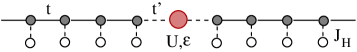
Figure 1: (Color online) Picture of model (1).

II Model and methods

Hence, in this article we will study a one-dimensional FKLM with an Anderson impurity located in the center of the chain (see Fig. 1). Then, the model is defined by the Hamiltonian:

$${\cal H}_{0}= - t_{0}\sum_{i>0,i<-1,\sigma}(c^{\dagger}_{i+1\sigma}c_{i\sigma}+H.c.)-J_{H}\sum_{l\neq 0}{\bf S}_{l}\cdot{\bf s}_{l}$$ (1)

$$- t^{\prime}\sum_{\sigma}(c^{\dagger}_{-1\sigma}c_{0\sigma}+c^{\dagger}_{1\sigma}c_{0\sigma}+H.c.)$$

$$+ Un_{0,\uparrow}n_{0,\downarrow}+\epsilon n_{0}$$

where the notation is standard. The Anderson impurity or “QD”, with parameters $U,\epsilon$, is located at site “0” and is connected to the rest of the system with a hopping $t^{\prime}$. The “leads” ($i\neq 0$) correspond to the FKLM with the Hund’s rule exchange coupling $J_{H}>0$. $S_{l}$ is the spin operator for the localized spin-1/2 orbital and $s_{l}$ is the one for the conduction electron at site $l$ ($l\neq 0$). $t_{0}=1$ is adopted as unit of energy, and we take $t^{\prime}=0.4$ throughout. Model (1) will be termed “QD-FKL” model.

The pure single-orbital FKLM or Kubo-Ohata modellamno has been extensively studied, particularly using numerical techniquesrierahallberg and its phase diagram for various spatial dimensions and values $S$ of the localized spins has been determined.dagotto Even in the simplest case of 1D and spin-1/2 localized spins, the model reproduces qualitatively the main features of manganites. In the following we will work in the metallic FM phase of the FKLM, typically, the density of conduction electrons $n\leq 0.6$, $J_{H}=20$ (all coupling constants are expressed in units of $t_{0}$). The on-site potential $\epsilon$ and Coulomb repulsion $U$ are the main variables whose effects we want to study. In a heterostructure $\epsilon$ would be fixed by chemistry but in a spin valve it would correspond to the gate voltage which can be varied at will. In order to detect any departure from the fully polarized FM state it is essential to work in the subspace of total $S^{z}=0$ (1/2) for even (odd) number of electrons.

We denote with $L$ the total length of the system including the impurity site. Open boundary conditions (OBC) were adopted in the lattices studied except otherwise stated. Small clusters with $L$ up to 12 will be studied using exact diagonalization (ED) with the Lanczos algorithm. Larger clusters will be solved using density matrix-renormalization group (DMRG).dmrgrev For calculations in the subspace of maximum total z-component of the spin, $S^{z}$, i.e., saturated ferromagnetism, we used completely independent ED and DMRG codes for the spinless fermion model. The ED and DMRG codes for the FKLM were thoroughly checked, in the first place by reproducing results in the literature. In the second place, by comparing results obtained by both techniques in small clusters and finally, by comparing results for large chains between FKLM and the spinless fermion model in the case of maximum $S^{z}$. Here we would like to stress the fact that convergence to the ground state, both with ED and in the diagonalization of the superblock Hamiltonian at each iteration of DMRG is extremely slow. This is already known for ED studies of the Hubbard model with very large $U/t$ and small doping, that is in the proximity of the Nagaoka phase. DMRG studies for the Kondo lattice model (KLM), with both ferro- and antiferro- magnetic exchange coupling, have been in general restricted to smaller chains than for the Hubbard model. In fact, even in 1D, the DMRG treatment of KLM has the level of difficulty of an interacting system on a two-leg ladder. The convergence is even worst for the FKLM where previous studies have been limited to $L\approx 36$ with a discarded weight of order $10^{-5}$.garcia Last but not least, the presence of impurities makes the convergence more difficult particularly for DMRG. In our calculations, with a retained number of $M\approx 400$, the truncation error is negligible ($\approx 10^{-14}$) for $L\approx 20$ in the regions close to saturated ferromagnetism but it drops to $\approx 10^{-10}$ in the nonmagnetic region. In the case of the spinless fermion model, for $L\approx 20$ and $M\approx 400$, the precision in energy is at least 12 digits. In the parameter regions where total spin $S$ takes its maximum possible value $S_{max}$, the energy in the $S^{z}=0$ subspace reproduces the value obtained in the $S^{z}=S_{max}$ subspace using the spinless fermion model within at least 9 digits. In any case, the limited precision within DMRG depends essentially on the lack of convergence in the diagonalization of the Hamiltonian.

The conductance will be estimated by a numerical setupalhassanieh ; schmitteckert in which a small bias voltage is applied to the left (L) and right (R) leads, with $\Delta V=V_{R}-V_{L}$, ($V_{R}=-V_{L}$), at time $t=0$. The current $J(t)$ induced by this voltage on each bond connecting the QD to the leads is computed with the time evolution formalism both within ED or DMRG.schollwock This numerical setup is equivalent to the systems which were treated analytically using the Keldysh Green functions formalism.wingreen These results for out-of equilibrium, with interacting QD, contain as particular cases the ones for noninteracting systems described by the Landauer formula.datta These analytical results, both for interacting and noninteracting QDs, were recovered using this numerical setup and time-dependent DMRG.cazalilla ; alhassanieh ; schmitteckert The advantage of this numerical procedure is that it can be extended with no formal limitations to study the case of interacting leadsqdhub as will be done in the present work.

In principle, one could adopt as a measure of the conductance the maximum of $J(t)/\Delta V$. It has been shown that this recipe provides correct results for the conductance when the maximum of $J(t)$ corresponds to a “plateau” which appears in high-precision calculations using the “adaptive” time-dependent-DMRG on large clusters.alhassanieh In the following we adopt the less precise “static” algorithmcazalilla which still gives qualitatively correct results, particularly if relatively small clusters are considered, but is much faster than the “adaptive” scheme, thus allowing to explore a wider range of couplings and densities. In the case of ED, the time evolution is exactly computed in the full Hilbert space of the system. The time-evolution of the ground state is given by $|\Psi(t+\tau)\rangle=e^{-i{\cal H}\tau}|\Psi(t)\rangle$, where ${\cal H}={\cal H}_{0}+V_{L}N_{L}+V_{R}N_{R}$, $N_{L}$, $N_{R}$ are the electron occupancies of the left and right leads respectively, and $|\Psi(t=0)\rangle=|\Psi_{0}\rangle$, ${\cal H}_{0}|\Psi_{0}\rangle=E_{0}|\Psi_{0}\rangle$. $|\Psi(t+\tau)\rangle$ was computed using the Krylov algorithm.manmana All the results reported below correspond to $\Delta V=0.01$, $\tau=0.1$.

The dynamical impurity magnetic susceptibility and dynamical magnetic structure factor (defined for convenience in Section IV) are computed within ED and DMRG using the standard continued fraction formalism. In the case of DMRG we again choose the “static” formulation which although less precise is enough to determine the presence or absence of a peak at the bottom of the spectrum.

We would like to stress that the most important results reported in this article correspond to static properties, that is, ground state energies and spin-spin correlations, where the precision of DMRG is maximal. For all quantities studied, the results obtained with ED are precise to precision machine.

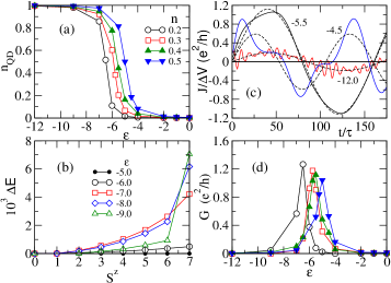
Figure 2: (Color online) (a) QD occupancy as a function of $\epsilon$, at several electron densities $n$. (b) $\Delta E=E(S^{z})-E(0)$, versus $S^{z}$, $n=0.5$. (c) $J(t)/\Delta V$ for $n=0.4$, $\epsilon=-4.5$, $-5.5$ and $-12$ (full curves). Sinusoidal fits are shown with dashed lines. Curves for $\epsilon=-4.5$ and $-12$ have been multiplied by 2 and 20 respectively. (d) Conductance, as a function of $\epsilon$, for the same electron densities as in (a). $L=10$, $J_{H}=20$, $t^{\prime}=0.4$, $\epsilon=-U/2$.

III Results at the symmetric point

Let us start to analyze results for the QD-FKL model in the $L=10$ cluster obtained by ED. We consider in the first place the case of the “symmetric point”, $\epsilon=-U/2$. The symmetric point of an Anderson impurity is in principle the obvious place to look for a magnetic impurity placed in a noninteracting chain. However, this is not the case for the present model. It can be seen in Fig. 2(a) that the QD or impurity occupancy, and hence its actual magnetic or nonmagnetic character, experiences a sharp crossover as a function of the on-site potential of the impurity. For values of $\epsilon$ larger than a crossover value $\epsilon^{*}$, $n_{QD}\approx 0$, and for values of $\epsilon<\epsilon^{*}$, $n_{QD}\approx 1$. $\epsilon^{*}$ may be defined as the value of $\epsilon$ at which $n_{QD}=0.5$. This crossover can be understood by examining two variational states in the atomic limit. One, with energy $E_{1}=-J_{H}n_{e}/4$, ($n_{e}$ is the number of conduction electrons) where all electrons are located on the leads and ferromagnetically aligned with the localized spins, and the other with energy $E_{2}=-J_{H}(n_{e}-1)/4+\epsilon$, where one electron has been moved from the leads to the QD. The crossover between both variational states at $\epsilon^{*}_{var}=-J_{H}/4$ is quite close to $\epsilon^{*}$ as shown in Fig. 2(a). The dependence of $\epsilon^{*}$ with $n$ is mainly due to the kinetic energy which can be easily computed within the spinless fermion model to which the FKLM is reduced in the saturated FM state, i.e. when total spin $S=S_{max}=S^{z}_{max}=n_{e}/2$. In this case, neglecting the term with $t^{\prime}$, $\epsilon^{*}_{spinless}$ is equal to the single particle energy of the top of the band which increases with $n$ and is exactly zero at $n=0.5$. The connection between both models implies that $\epsilon_{spinless}=\epsilon+J_{H}/4$.

It is important to notice at this point that although the pure system is in the saturated FM state for the densities studied, for some impurity parameters the impurity may drive the system into partially polarized FM states with total spin $S<S_{max}$. In fact, as shown in Fig. 2(b) for $n=0.5$, there is a region of $\epsilon$, close to $\epsilon^{*}$, where $S=0$ ($1/2$) for even (odd) $n_{e}$. We have observed this nonmagnetic state for other chain lengths and densities. Although the difference in energy between states with different $S^{z}$ is very small, these results strongly suggest that there are regions in parameter space where the impurity causes a breakdown of the fully saturated FM state. This possibility will be thoroughly examined in the next Section.

Let us discuss in detail how the conductance $G$ is determined. In Fig. 2(c), it is shown $J(t)/\Delta V$ ($J(t)$ is the average of the current on the two bonds connecting the QD to the leads) which presents the typical oscillatory behavior. This oscillatory behavior follows from the expansion of $e^{-i{\cal H}\tau}$ in eigenvectors of ${\cal H}$, which for small $\Delta V$ are adiabatically related to those of ${\cal H}_{0}$. We would like to emphasize that results depicted in Fig. 2(c) are exact, i.e., no truncation of the Hilbert space was performed. Then, we fit each curve by a sinusoidal and we adopt $G$ as the amplitude of this sinusoidal. In this small cluster, but also for $L=20$, a single sinusoidal gives a reasonable fitting of $J(t)/\Delta V$ for most of the cases studied, particularly near $\epsilon^{*}$. Although this procedure is not very precise, it gives qualitatively correct results as we discuss in the following.

Results for the conductance are shown in Fig. 2(d) for various densities as a function of $\epsilon$. $G$ is only different from zero at the crossover between the region of empty QD ($\epsilon>>\epsilon^{*}$) and the region of half-filled QD ($\epsilon<<\epsilon^{*}$) and it has a sharp peak at $\epsilon^{*}$ with a width approximately equal to the bandwidth of a tight-binding model on the leads, $4t_{0}$. This behavior is what one would expect for the spinless fermion model. The determination of the variation of the maximum conductance with density $n$, which would require calculations on a finer mesh in $\epsilon$, is out of the scope of the present study.

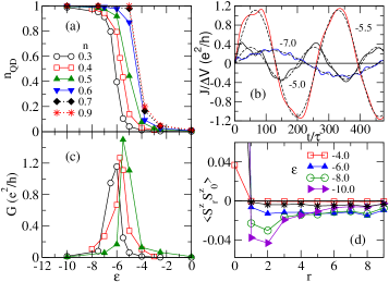
Figure 3: (Color online) (a) QD occupancy and (c) conductance, as a function of $\epsilon$, for several electron densities $n$ indicated on the plot. (b) $J(t)/\Delta V$ for $n=0.4$, $\epsilon=-5$, $-5.5$ and $-7$ (full curves). Fits to a sine function are shown with dashed lines. Results for $L=20$, $J_{H}=20$, $t^{\prime}=0.4$, $\epsilon=-U/2$. (d) Spin-spin correlations along the conduction chain, for the pure FKLM (stars) and in the presence of an impurity for various values of $\epsilon$ indicated on the plot, $L=19$, $n=0.421$. The reference site is located at the center of the chain and the normalization $\langle S^{z}_{0}S^{z}_{0}\rangle=1$ was adopted.

Let us now discuss results for $L=20$, obtained with DMRG, also at the symmetric point. In Fig. 3(a), it can be seen that, as for $L=10$, the impurity occupancy $n_{QD}$ experiences a sudden change as a function of the on-site potential $\epsilon$. This crossover is located approximately at $\epsilon^{*}=-J_{H}/4$ as argued before, even inside the incommensurate (IC) phase (but not strictly at $n=1$), which is expected since the variational states are independent of the underlying FM or IC order. As in the $L=10$ cluster, the location of this crossover shifts to larger values of $\epsilon$ as the density is increased. At the IC-FM crossover for $J_{H}=20$, $n\approx 0.55$, $\epsilon^{*}$ experiences a somewhat larger increase and then it remains relatively unchanged up to half-filling. In the IC region of course the kinetic energy is no longer approximated by the spinless fermion model. In fact, it is easy to realize that the kinetic energy versus $\epsilon$ follows an opposite behavior as the IC-FM border is crossed.

The computation of the conductance follows the steps previously outlined. In Fig. 3(b), $J(t)/\Delta V$ is shown for $n=0.4$ and several values of $\epsilon$. It can be seen that in spite of the approximate nature of the computation of the time evolution in a truncated Hilbert space, $J(t)$ is clearly well fitted by a single sinusoidal, particularly close to $\epsilon^{*}$, and these oscillations have similar behaviors as a function of $\epsilon^{*}$ as earlier for the $L=10$ chain. In Fig. 3(c) we show the resulting $G$ as a function of $\epsilon$ and for several densities. As for the smaller lattice $L=10$, the conductance is different from zero only for $\epsilon\approx\epsilon^{*}$, with a peak at $\epsilon^{*}$.note2

In spite of the extremely slow convergence in DMRG calculations, by keeping 450 states we were able to find that $E(S^{z}=0)<E(S^{z}=S_{max})$ for $\epsilon=-8$, thus suggesting for $L=19$ a similar behavior to that shown in Fig. 2(c) for $L=10$. Further indications of this behavior can be obtained by examining the $z$-component of the spin-spin correlations $\langle S^{z}_{j}S^{z}_{0}\rangle$, where the reference site “0” is the center of the chain and $j$ labels conduction sites. Due to the large value of $J_{H}$, the correlations between the impurity site and the localized spins have the same qualitative behavior so in this and in the following section we will only consider the correlations between the impurity and the conduction sites. These correlations, shown in Fig. 3(d) for $n=0.421$, clearly depart from the correlations in the pure system as $|\epsilon|$ is increased. This behavior indicates that the ground state computed by DMRG is a mixture of states very close in energy which depart from the saturated FM state. Then, this behavior of $\langle S^{z}_{j}S^{z}_{0}\rangle$ with $\epsilon$, which follows the same trend as the one for the $L=10$ chain, suggests that also for the $L=19$ chain the ground state $S<S_{max}$. Notice also that in this low-$S$ region, $\langle S^{z}_{j}S^{z}_{0}\rangle$ do not show any trace of antiferromagnetic order.

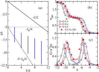
Figure 4: (Color online) (a) Variational states for model Eq. (1) in the $U$-$\epsilon$ plane. Vertical thick lines indicate approximately the region with minimum $S$ for some values of $U$, $n=0.4$, discussed in the text. (b) QD occupancy and (c) conductance as a function of $\epsilon$, for $U=4$, and various electron fillings $n$. Results for $L=10$ chain except otherwise stated.

IV Breakdown of the ferromagnetic state away from the symmetric point

Let us discuss the consequences of these results for devices where the leads are made with manganites. Since $J_{H}/t_{0}$ in manganites has been estimated of the order or larger than 10,lamno ; dagorep then a value of $U^{*}=-2\epsilon^{*}\geq 5$ in the QD (see Fig. 4(a)) would be required for $n_{QD}\sim 1$. This value of $U$ is somewhat larger than the one in materials employed in the QD, such as semiconductors or carbon nanotubes. It is necessary then that the device could be operated away from the symmetric point. More importantly, a smaller $U$ could imply a larger effective coupling between the impurity and the conduction sites, assuming that to lowest approximation the relation $J_{eff}\approx t^{\prime 2}/U$ is still valid for the present model for $U>t^{\prime}$. In support of this hypothesis, we have observed that the spin-spin correlation between the impurity and its nearest neighbor site becomes more negative with decreasing $U$ at fixed $\epsilon$. Then, by working with a larger $J_{eff}$ we could expect to be more able to detect the presence of the nonmagnetic phase which was suggested by the results found in the previous section. For these reasons, in the following we adopt a moderate value of the on-site Coulomb repulsion, $U=4$, and we study the properties of the model for variable $\epsilon$, i.e. following a vertical line in Fig. 4(a).

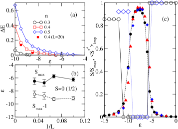
Figure 5: (Color online) (a) $\Delta E=E(S^{z}_{max})-E(S^{z}_{min})$, as a function of $\epsilon$, for $U=4$, and various electron fillings $n$. Results for $L=10$ chain except otherwise stated. (b) Upper (solid line) and lower (dashed line) boundaries of the region where the ground state $S=0(1/2)$, for $n=0.4$, as a function of $L$, for $U=4$, and $n=0.4$. (c) $<S^{z^{2}}>$ (normalized to 1) at the impurity site (full symbols) and total spin normalized to $S_{max}$ (open symbols), as a function of $\epsilon$, for $U=4$. Results for $L=11$, $n=0.364$ (circles), $L=19$, $n=0.421$ (diamonds), and $L=20$, $n=0.4$ (triangles).

The electron occupancy at the QD, shown in Fig. 4(b) for $L=10$, presents now three regions where $n_{QD}$ is approximately 0, 1, and 2 as $\epsilon$ decreases. The crossovers among these regions are located near the variational estimates $\epsilon^{*}_{0,1}\approx-J_{H}/4$, and $\epsilon^{*}_{1,2}\approx-J_{H}/4-U$ which are shown in Fig. 4(a). As it can be seen in Fig. 4(c), the conductance $G$ consistently with the results shown in Figs.  2(d) and  3(c) at the symmetric point, presents sharp peaks at the crossovers between regions with different $n_{QD}$, i.e. when $n_{QD}\approx 0.5$ or $1.5$. Notice that $G$ has a larger value between the peaks for $n=0.4$ compared with the one for $n=0.3$, which is essentially zero.

Figure 5 contains the most important result of our work. In Fig. 5(a) we plot $\Delta E=E(S^{z}_{max})-E(S^{z}_{min})$, where $S_{min}=S^{z}_{min}=0$ ($1/2$) for even (odd) $n_{e}$, as a function of $\epsilon$ in the $L=10$ chain. It can be clearly seen that the ground state $S$ is smaller than $S_{max}$ for the various densities considered for $\epsilon\leq\epsilon^{*}_{0,1}$. In this case, $\Delta E$ is quite large and we were able to obtain for $L=20$ results very close to those for $L=10$, as shown for $n=0.4$, suggesting that this feature is at least not an artifact of this small chain. More interesting is the fact that inside the $n_{QD}=1$ region there is an interval in $\epsilon$, which depends on the density, where $S=S_{min}$, as shown in Fig. 5(b) for $n=0.4$ as a function of $1/L$. This state appears between two saturated FM states, $S=S_{max}-1$ below the lower boundary line because of the double occupancy of the QD, and $S=S_{max}$ above the upper boundary line where the QD is empty. The error bars quoted in the plot correspond to the grid adopted in the $\epsilon$ axis. For the largest chain studied, $L=30$, we have only computed the energies in the $S^{z}=S_{max}$, $S_{max}-1$, $S_{max}-2$ and $S_{max}-3$ subspaces. Decreasing precision as $L$ increases prevents us to take a finer grid close to the crossover between different regions and hence error bars are larger. An extrapolation to the bulk limit would not be reliable with these error bars. For $L=10$, $n=0.3$, the region in $\epsilon$ where $S=1/2$ shrinks to $[-9.3,-8.6]$. It is tempting to relate this smaller interval for $n=0.3$ with respect to the one for $n=0.4$ with the behavior of $G$ noticed above but further analysis would be needed to confirm this possibility. In Fig. 5(c) we show that the presence of a state with $S=S_{min}$ corresponds to a strong magnetic character of the impurity with $<S^{z^{2}}>$ approaching its maximum value of one (according to the normalization adopted). This feature has been observed for all lattices, densities, and values of $U$ studied. The intervals in $\epsilon$ where $S=S_{min}$ for various values of $U$, $n=0.4$, $L=10$ are shown in Fig. 4(a) with thick lines.

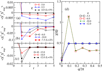
Figure 6: (Color online) Spin-spin correlations from the impurity site along the conduction chain for several values of $\epsilon$ in the regions where (a) $S=S_{max}$, (b) $S=0$, and (c) $S=S_{max}-1$. The normalization $\langle S^{z}_{0}S^{z}_{0}\rangle=1$ was adopted. (d) Static structure factor along the conduction chain for various values of $\epsilon$. Results for $L=11$ chain, PBC, $U=4$, $n=0.364$, except otherwise stated. Results for $L=19$ correspond to $n=0.421$ and for $L=25$ $n=0.4$.

The behavior of the magnetic character of the impurity affects in turn all the magnetic properties in the system. Let us first examine the spin-spin correlations between the impurity site and the remaining sites along the conduction chain. Results for the $L=11$ chain with periodic boundary conditions (PBC), $n=0.364$, are shown in Fig. 6(a), (b) and (c) in the three regions where the spin of the ground state is $S_{max}$, 0 and $S_{max}-1$, respectively. We also included in this figure results for $L=19$, $n=0.421$, and $L=25$, $n=0.4$, OBC, which show the same behavior. It should be noticed that in addition to the expected larger magnitude of these correlations in the $S=0$ region with respect to the ones in the other two regions, there are also qualitative changes. To detect these qualitative differences we have computed the static structure factor along the conduction chain:

$$\chi(q)=\frac{1}{L}\sum_{l,j}\langle S^{z}_{l}S^{z}_{j}\rangle e^{iq(l-j)}$$ (2)

where $j,l$ label the conduction chain sites, and $q=(2\pi/L)n$, $n=0,\ldots,L-1$ . Results where site $j$ is restricted to the impurity site, that is just the Fourier transform of the correlations shown in Fig. 6(a), (b) and (c), are essentially the same as those obtained using Eq. (2). As it can be seen in Fig. 6(d), $\chi(q)$ has the typical shape of a FM order in the subspace of total $S^{z}=0$ in the regions with $S=S_{max}$ and $S_{max}-1$, while it presents a peak at the smallest nonzero momentum in the region $S=0$. As observed earlier, in Fig. 3(d), there are no traces of AF order in this region.

Further information about changes in magnetic properties caused by the impurity can be obtained by looking at the dynamical impurity susceptibility defined as:

$$S_{imp}(\omega)=\sum_{n}|\langle\Psi_{n}|S^{z}_{imp}|\Psi_{0}\rangle|^{2}\delta(\omega-(E_{n}-E_{0}))$$ (3)

where the notation is standard. Since the contribution from the remaining sites on the conduction chain is negligible, $S_{imp}(\omega)$ is essentially equal to the total dynamical susceptibility once the contribution from localized spins has been subtracted. In all results below, the peaks have been broadened with a width $\delta=0.1$.

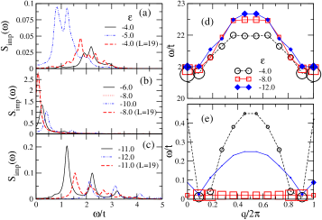
Figure 7: (Color online) Dynamical impurity susceptibility $S_{imp}(\omega)$ vs $\omega$ for $U=4$, $n=0.4$, and values of $\epsilon$ in the region where (a) $S=S_{max}$, (b) $S=0$, and (c) $S=S_{max}-1$. Energies of the dominant peaks in the dynamical structure factor $\chi(q,\omega)$, (d) in the high- and (e) in the low-$\omega$ regions as defined in the text for various values of $\epsilon$. The size of the symbols is proportional to the intensity of each peak. Results for $L=11$ chain except otherwise stated.

In Fig. 7(a), (b) and (c) we show $S_{imp}(\omega)$ in the low-$\omega$ part of the spectrum for various values of $\epsilon$ in the regions $S=S_{max}$, 0 and $S_{max}-1$ respectively, for $L=11$, $n=0.4$ and $L=19$, $n=0.421$. Again, in addition to an expected difference in amplitude, a clear qualitatively different behavior is noticeable. In this part of the spectrum $S_{imp}(\omega)$ presents small peaks at finite $\omega$ in the $S=S_{max}$ and $S_{max}-1$ regions while in the $S=0$ region, $S_{imp}(\omega)$ shows a strong peak close to $\omega=0$. Results for $L=25$, $n=0.4$, $\epsilon=-8$ are indistinguishable from those for $L=19$.

The distinct behavior caused by the impurity can also be detected by looking at the dynamical structure factor on the conduction chain which is defined as:

$$\chi(q,\omega)=\sum_{n}|\langle\Psi_{n}|S^{z}_{q}|\Psi_{0}\rangle|^{2}\delta(\omega-(E_{n}-E_{0}))$$ (4)

where $S^{z}_{q}=(1/L)\sum_{j}S^{z}_{j}\exp{(ijq)}$, and the sum extends over the conduction chain. Figure 7(d) and (e) show the energy and intensity of the centroid of the main peaks in the high- and low-$\omega$ parts of the spectrum for values of $\epsilon$ in the three regions of total spin $S$ above discussed. In the $S=S_{max}$ and $S_{max}-1$ regions the peaks with largest weight are those with energy close to $J_{H}$ which corresponds to the magnon excitation. This behavior is strikingly different to the one in the $S=0$ region where the most weighted peak form a dispersionless band at the bottom of the spectrum. This band is reminiscent of the one found in gapped spin systems upon doping with nonmagnetic impurities.martins In the present case, these low-energy peaks may correspond to magnetic excitations living in a “cloud” surrounding the impurity that can be observed in real-space in Fig. 6(b).

V Discussion and conclusions

We have applied both well-established and recently developed numerical approaches to study the FKLM with an Anderson impurity in the FM phase on finite chains. We found that the magnetic or nonmagnetic character of the impurity is determined by a relationship between the impurity parameters and the Hund’s rule exchange coupling of the manganite. As expected, transport occurs at the crossovers between the empty, half-filled or filled QD regions.

The most important result of this article is the presence of an intermediate singlet phase between the fully saturated phases with $S_{max}$ (empty impurity) or $S_{max}-1$ (doubly occupied impurity). This problem has some resemblance with the problem of the existence of an intermediate phase between two ordered states in the frustrated Heisenberg model on the square lattice. This intermediate phase had been predicted by ED studies on small clusters.j1j2inter The alternative view was a first order quantum phase transition between both ordered phases. Only recently was this controversy being settled favouring the existence of the intermediate statej1j2fin but the nature of this phase is still a subject of active research.j1j2nuevo Of course the physics involved in both problems is completely different, but by analogy, in our problem, we could consider the possibility of a first-order transition between two FM states instead of the proposed intermediate nonmagnetic phase. By comparing the models involved in these two problems, FKLM and frustrated Heisenberg model, the former is much more difficult to analyze than the latter by numerical techniques since the size of the Hilbert space is much larger for a given cluster and moreover taking into account the convergence problems discussed in Section II. These difficulties prevent us to perform an extrapolation in order to decide if this intermediate phase really exists in the bulk limit or if it is just how the transition between the $S_{max}$ and $S_{max}-1$ phases manifests in finite systems.

In any case, the possibility of the existence of this intermediate state is in principle interesting and important and it deserves further study. In this sense, there are three issues that should be considered. The first one is that this intermediate phase could be stabilized by some modifications of the model, for example by including the Heisenberg interaction between localized spins, or by replacing the spin-1/2 localized spins by higher spin ones which, in addition, are also more realistic for manganites. The second issue is that even if this intermediate phase has a finite range around an impurity, a finite density of impurities could lead to a macroscopic feature. The situation here is analog to the presence of nonmagnetic impurities in the above mentioned gapped systems.martins In these systems a single impurity attracts locally a spinon to the impurity and a finite density of impurities drives the system to a long-range AF order. These two issues are currently under study.largo The third issue we would like to consider is related to the relevance of the present model to devices with finite dimensions. In these mesoscopic systems, as discussed in introductory textbooks,datta due to its finite size, many physical properties are different to that found in bulk systems. It is then relevant for these devices to capture short-range effects.

Finally, we would like to provide a qualitative scenario to help understanding this nonmagnetic state. Let us assume that the system is in a low $S^{z}$ state. In the region where the impurity is empty or double occupied, both “leads” are relatively disconnected and each one would have a ferromagnetic state with spins polarized in one direction and the other with spins polarized in the opposite direction. Of course this state is degenerate with the one with reversed polarizations. Now, when the impurity is singly occupied, not only it would have a definite magnetic character but it would allow the crossing of one electron from one lead to the other where it would have then a “wrong” spin. This kind of magnons would then decrease the total energy both by increasing the kinetic energy and by decreasing the magnetic energy due to an effective AF interaction with the impurity. Of course, this gain in energy would not occur for the fully polarized system so it would drive the system to lower $S$ and presumably to $S_{min}$.note3 It is interesting to notice that this scenario would then imply an enhancement of transport in the system which could be relevant for the devices mentioned in the Introduction.

In summary, we present a prediction on the magnetic state of the FKLM doped with a magnetic impurity. This prediction could be experimentally verified on Cu-doped manganite nanotubes. These results could also be in principle reproduced experimentally on spin valves where manganites are used as ferromagnetic leads. We hope the present results will encourage theoretical studies to further characterize this proposed intermediate phase and to explore its presence in more realistic models for manganites.

- (1) M. B. Salamon and M. Jaime, Rev. Mod. Phys 73, 583 (2001); T. Kaplan and S. Mahanti, (eds.), Physics of Manganites, (Kluwer Academic/Plenum Publishers, New York, 1999).
- (2) E. Dagotto, T. Hotta, and A. Moreo, Phys. Rep. 344, 1 (2001).
- (3) A. P. Ramirez, J. Phys.: Condens. Matter 9, 8171 (1997), and references therein.
- (4) I. Žutic, J. Fabian, and S. Das Sarma, Rev. Mod. Phys. 76, 323 (2004).
- (5) M. Bibes and A. Barthélémy, IEEE Trans. Electron. Devices 54, 1003 (2007).
- (6) R. Hanson, L. P. Kouwenhoven, J. R. Petta, S. Tarucha, and L. M. K. Vandersypen, Rev. Mod. Phys. 79, 1217 (2007).
- (7) A. N. Pasupathy, R. C. Bialczak, J. Martinek, J. E. Grose, L. A. K. Donev, P. L. McEuen, and D. C. Ralph, Science 306, 86 (2004).
- (8) J. Martinek, M. Sindel, L. Borda, J. Barnas, J. König, G. Schön, and J. von Delft, Phys. Rev. Lett. 91, 247202 (2003)
- (9) C. J. Gazza, M. E. Torio, and J. A. Riera, Phys. Rev. B 73, 193108 (2006).
- (10) L. E. Hueso, J. M. Pruneda, V. Ferrari, G. Burnell, J. P. Valdes-Herrera, B. D. Simons, P. B. Littlewood, E. Artacho, A. Fert, N. D. Mathur, Nature 445, 410 (2007).
- (11) A. Cottet, T. Kontos, S. Sahoo, H. T. Man, M-S. Choi, W. Belzig, C. Bruder, A. Morpurgo, C. Schoenenberger, Semicond. Sci. Technol. 21, S78 (2006).
- (12) C. H. Ahn, A. Bhattacharya, M. Di Ventra, J. N. Eckstein, C. D. Frisbie, M. E. Gershenson, A. M. Goldman, I. H. Inoue, J. Mannhart, A. J. Millis, A. F. Morpurgo, D. Natelson, J.-M. Triscone, Rev. Mod. Phys. 78, 1185 (2006).
- (13) Cr-doped manganites have already been studied but Cr-ions are not described as an Anderson impurity. See e.g., T. Kimura, Y. Tokura, R. Kumai, Y. Okimoto, and Y. Tomioka, J. Appl. Phys. 89, 6857 (2001).
- (14) G. B. Martins, E. Dagotto and J. A. Riera, Phys. Rev. B 54, 16032 (1996); G. B. Martins, M. Laukamp, J. Riera, and E. Dagotto, Phys. Rev. Lett. 78, 3563 (1997).
- (15) A. J. Hewson, The Kondo problem to heavy fermions, (Cambridge University Press, Cambridge, UK, 1993).
- (16) J. Riera, K. Hallberg and E. Dagotto, Phys. Rev. Lett. 79, 713 (1997).
- (17) E. Dagotto, S. Yunoki, A. L. Malvezzi, A. Moreo, J. Hu, S. Capponi, D. Poilblanc, and N. Furukawa, Phys. Rev. B 58, 6414 (1998).
- (18) U. Schollwöck, Rev. Mod. Phys. 77, 259 (2005).
- (19) D. J. García, K. Hallberg, B. Alascio, and M. Avignon, Phys. Rev. Lett. 93, 177204 (2004).
- (20) K. A. Al-Hassanieh, A. E. Feiguin, J. A. Riera, C. A. Büsser, and E. Dagotto, Phys. Rev. B 73, 195304 (2006).
- (21) P. Schmitteckert, Phys. Rev. B 70, 121302 (2004).
- (22) U. Schollwöck, J. Phys. Soc. Jpn. 74 (Suppl.), 246 (2005), and references therein.
- (23) Y. Meir and N. S. Wingreen, Phys. Rev. Lett. 68, 2512 (1992); N. S. Wingreen, A. P. Jauho, and Y. Meir, Phys. Rev. B 48, 8487 (1993).
- (24) S. Datta, Electronic transport in mesoscopic systems (Cambridge University Press, Cambridge, 1995).
- (25) M. A. Cazalilla and J. B. Marston, Phys. Rev. Lett. 88, 256403 (2002).
- (26) S. Costamagna, C. J. Gazza, M. E. Torio, and J.A. Riera, Phys. Rev. B 74, 195103 (2006).
- (27) S. R. Manmana, A. Muramatsu, and R. M. Noack, AIP Conf. Proc. 789, 269-278 (2005).
- (28) For chains with odd, we obtain that the conductance maximum is located at values of lower (higher) than for even (odd) number of conduction electrons. However, the results for odd converge to those of even as the chain length is increased.
- (29) J. E. Hirsch and S. Tang, Phys. Rev. B 39, 2887 (1989); M. P. Gelfand, R. R. P. Singh, and D. A. Huse, 40, 10801 (1989).
- (30) R. R. P. Singh, Z. Weihong, C. J. Hamer, and J. Oitmaa, Phys. Rev. B 60, 7278 (1999); S. Kurata, C. Sasaki, and K. Kawasaki, Phys. Rev. B 63, 024412 (2000).
- (31) V. Lante and A. Parola, Phys. Rev. B 73, 094427 (2006).
- (32) S. Costamagna and J. A. Riera, in preparation.
- (33) Preliminary calculations show that the magnetic energy decreases strongly than the increase of kinetic energy as is reduced.