On Fast-Decodable Space–Time Block Codes

Abstract

We focus on full-rate, fast-decodable space–time block codes (STBCs) for $2\times 2$ and $4\times 2$ multiple-input multiple-output (MIMO) transmission. We first derive conditions and design criteria for reduced-complexity maximum-likelihood decodable $2\times 2$ STBCs, and we apply them to two families of codes that were recently discovered. Next, we derive a novel reduced-complexity $4\times 2$ STBC, and show that it outperforms all previously known codes with certain constellations.

I Introduction

In 1998, Alamouti [1] invented a remarkable scheme for multiple-input multiple-output (MIMO) transmission using two transmit antennas and admitting a low-complexity maximum-likelihood (ML) decoder. Space–time block codes (STBCs) using more than two transmit antennas were designed in [17]. For such codes, ML decoding is achieved in a simple way, but, while they can achieve maximum diversity gain [5, 18], their transmission rate is reduced. The quasi-orthogonal STBCs in [9] can support a transmission rate larger than orthogonal STBCs, but at the price of a smaller diversity gain. Using algebraic number theory and cyclic division algebras, algebraic STBCs can be designed to achieve full rate and full diversity, but at the price of a higher decoding complexity.

Recently, a family of $2\times 2$ twisted space–time transmit diversity STBCs, having full rate and full diversity, was proposed in [19, 20, 7, 8]. These codes were recently rediscovered in [13], whose authors also pointed out that they enable reduced-complexity ML decoding (see infra for a definition of decoding complexity). Independently, the same codes were found in [14]. More recently, another family of full-rate, full-diversity, fast-decodable $2\times 2$ codes for MIMO was proposed in [16].

Empirical evidence seems to show that the constraint of simplified ML decoding does not entail substantial performance loss. To substantiate the above claim, the present paper provides a unified view of the fast-decodable STBCs in [19, 20, 7, 13, 14, 16] for $2\times 2$ MIMO. We show that all these codes allow the same low-complexity ML decoding procedure, which we specialize in the form of a sphere-decoder (SD) search [4, 15, 21, 22]. We also derive general design criteria for full-rate, fast-decodable STBCs, and we use it to design a family of $4\times 2$ codes based on a combination of algebraic and quasi-orthogonal structures. In this case, the full-diversity assumption is dropped in favor of simplified maximum-likelihood decoding. Within this family, we exhibit a code that outperforms all previously proposed $4\times 2$ STBCs for $4$-QAM signal constellation.

The balance of this paper is organized as follows. Section II introduces system model and code design criteria. In Section III, we present the concept of the fast-decodability of STBCs. In Section IV we review two families of fast-decodable $2\times 2$ STBCs recently appeared in the literature, and we show how both of them enable a reduced-complexity ML decoding procedure. In Section V, we propose fast-decodable $4\times 2$ STBCs, and we show the corresponding ML decoding complexity. Finally, conclusions are drawn in Section VI.

Notations: Boldface letters are used for column vectors, and capital boldface letters for matrices. Superscripts ^T, ^†, and ^∗ denote transposition, Hermitian transposition, and complex conjugation, respectively. $\mathbb{Z}$, $\mathbb{C}$, and $\mathbb{Z}[j]$ denote the ring of rational integers, the field of complex numbers, and the ring of Gaussian integers, respectively, where $j^{2}=-1$. Also, $\mathbf{I}_{n}$ denotes the $n\times n$ identity matrix, and $\mathbf{0}_{m\times n}$ denotes the $m\times n$ matrix all of whose elements are $0$.

Given a complex number $x$, we define the $\tilde{(\cdot)}$ operator from $\mathbb{C}$ to $\mathbb{R}^{2}$ as $\tilde{x}\triangleq[\Re(x),\Im(x)]^{T},$ where $\Re{(\cdot)}$ and $\Im{(\cdot)}$ denote real and imaginary parts. The $\tilde{(\cdot)}$ operator can be extended to complex vectors $\mathbf{x}=[x_{1},\ldots x_{n}]\in\mathbb{C}^{n}$:

$$\tilde{\mathbf{x}}\triangleq[\Re(x_{1}),\Im(x_{1}),\ldots,\Re(x_{n}),\Im(x_{n})]^{T}$$

Given a complex number $x$, the $\check{(\cdot)}$ operator from $\mathbb{C}$ to $\mathbb{R}^{2\times 2}$ is defined by

$$\check{x}\triangleq\left[\begin{array}[]{cc}\Re(x)&-\Im(x)\\ \Im(x)&\Re(x)\end{array}\right]$$

The $\check{(\cdot)}$ operator can be similarly extended to $n\times n$ matrices by applying it to all the entries, which yields $2n\times 2n$ real matrices. The following relations hold: $\widetilde{\mathbf{Ax}}=\check{\mathbf{A}}\tilde{\mathbf{x}}$ and $\mathbf{A}=\mathbf{B}\mathbf{C}\Longrightarrow\check{\mathbf{A}}=\check{\mathbf{B}}\check{\mathbf{C}}$. Given a complex number $x$, we define the $\bar{\check{(\cdot)}}$ operator from $\mathbb{C}$ to ${\mathbb{R}}^{2\times 2}$ as

$$\bar{\check{x}}\triangleq\left[\begin{array}[]{cc}-\Re(x)&-\Im(x)\\ -\Im(x)&\Re(x)\end{array}\right]$$

The following relation holds:

$$\widetilde{xy^{*}}\triangleq\bar{\check{x}}\cdot\tilde{y}$$

The ${\rm vec}(\cdot)$ operator stacks the $m$ column vectors of a $n\times m$ complex matrix into a $mn$ complex column vector. The $\|\cdot\|$ operation denotes the Euclidean norm of a vector. Finally, the Hermitian inner product of two complex column vectors $\mathbf{a}$ and $\mathbf{b}$ is denoted by $\langle\mathbf{a},\mathbf{b}\rangle\triangleq\mathbf{a}^{T}\mathbf{b}^{*}$. Note also that if $\langle\mathbf{a},\mathbf{b}\rangle=0$, then $\langle\tilde{\mathbf{a}},\tilde{\mathbf{b}}\rangle=0$.

II System Model and Code Design Criteria

We consider a $n_{r}\times n_{t}$ MIMO transmission over a block-fading channel. The received signal matrix ${\mathbf{Y}}\in\mathbb{C}^{n_{r}\times T}$ is

$${\mathbf{Y}}={\mathbf{H}}{\mathbf{X}}+{\mathbf{N}}$$ (1)

where $\mathbf{X}\in\mathbb{C}^{n_{t}\times T}$ is the codeword matrix, transmitted over $T$ channel uses. Moreover, ${\mathbf{N}}\in\mathbb{C}^{n_{r}\times T}$ is a complex white Gaussian noise with i.i.d. entries $\sim{\mathcal{N}}_{\mathbb{C}}(0,N_{0})$, and $\mathbf{H}=[h_{i\ell}]\in\mathbb{C}^{n_{r}\times n_{t}}$ is the channel matrix, assumed to remain constant during the transmission of a codeword, and to take on independent values from codeword to codeword. The elements of $\mathbf{H}$ are assumed to be i.i.d. circularly symmetric Gaussian random variables $\sim{\mathcal{N}}_{\mathbb{C}}(0,1)$. The realization of $\bf H$ is assumed to be known at the receiver, but not at the transmitter. The following definitions are relevant here:

Definition 1

(Code rate) Let $\kappa$ be the number of independent information symbols per codeword, drawn from a complex constellation ${\mathcal{S}}$. The code rate of a STBC is defined as $R=\kappa/T$ symbols per channel use. If $\kappa=n_{r}T$, the STBC is said to have full rate. $\hfill\square$

Consider ML decoding. This consists of finding the code matrix that achieves the minimum of the squared Frobenius norm $m({\bf X})\triangleq\|{\bf Y-HX}\|^{2}$.

Definition 2

(Decoding Complexity) The ML decoding complexity is defined as the minimum number of values of $m(\bf X)$ that should be computed in ML decoding. This number cannot exceed $M^{\kappa}$, with $M=|{\mathcal{S}}|$, the complexity of the exhaustive-search ML decoder. $\hfill\square$

Consider two codewords $\mathbf{X}$ and $\widehat{\mathbf{X}}\neq{\bf X}$. Let $r$ denote the minimum rank of the matrix $\mathbf{X}-\widehat{\mathbf{X}}$, and $\delta$ the product distance, i.e., the product of non-zero eigenvalues of the codeword distance matrix $\mathbf{E}\triangleq(\mathbf{X}-\widehat{\mathbf{X}})(\mathbf{X}-\widehat{\mathbf{X}})^{\dagger}$. The error probability of a STBC is upper bounded by the following union bound,

$$P(e)\leq\frac{1}{M^{\kappa}}\sum_{r}\sum_{\delta}A(r,\delta)P(r,\delta)$$ (2)

where $P(r,\delta)$ denotes the pairwise error probability (PEP) of the codeword differences with rank $r$ and product distance $\delta$, and $A(r,\delta)$ the associated multiplicity. In [18], the “rank-and-determinant criterion” (RDC) was proposed to maximize both the minimum rank $r$ and the minimum determinant $\delta_{\min}\triangleq\underset{\mathbf{X}\neq\widehat{\mathbf{X}}}{\min}\det\left(\mathbf{E}\right)$. For a full-diversity STBC, i.e., $r=n_{t}$ for all $\mathbf{E}$ matrices, this criterion yields diversity gain $n_{r}n_{t}$ and coding gain $\left(\delta_{\min}\right)^{\frac{1}{n_{t}}}$ [18]. For STBC with $\delta_{\min}=0$, and hence without full diversity, one should minimize $A(r,\delta)$ with $r\leq n_{t}$.

II-A Linear codes, and Codes with the Alamouti structure

Linear STBCs are especially relevant in our context, because they admit ML sphere decoding.

Definition 3

(Linear STBC) A STBC carrying $\kappa$ symbols $\mathbf{s}=[s_{1},\ldots,s_{\kappa}]$ is said to be (real) linear if we can write $\widetilde{\mbox{vec}(\mathbf{X})}=\mathbb{G}\tilde{\mathbf{s}}$ for some $\mathbb{G}\in\mathbb{R}^{2n_{t}T\times 2\kappa}$. The matrix $\mathbb{G}$ is called the (real) generator matrix of the linear code. If a complex matrix $\mathbf{G}\in\mathbb{C}^{n_{t}T\times\kappa}$ exists such that $\mathbb{G}=\check{\mathbf{G}}$, then we can write $\mbox{vec}(\mathbf{X})=\mathbf{G}\mathbf{s}$ which identifies a complex linear STBC, with $\mathbf{G}$ its complex generator matrix. $\hfill\square$

Definition 4

(Cubic shaping) For a linear STBC, if its real generator matrix $\mathbb{G}$ is an orthogonal matrix satisfying $\mathbb{G}^{\dagger}\mathbb{G}=\mathbf{I}_{2\kappa}$, then we say that the STBC has cubic shaping (see [12] for the significance of cubic shaping). $\hfill\square$

Linear STBCS admit the canonical decomposition

$${\bf X}=\sum_{\ell=1}^{\kappa}(a_{\ell}{\bf A}_{\ell}+jb_{\ell}{\bf B}_{\ell})$$ (3)

where $a_{\ell}$ and $b_{\ell}$ are the real and imaginary part of $s_{\ell}$, respectively, and ${\bf A}_{\ell},{\bf B}_{\ell}$, $\ell=1,\ldots,\kappa$, are $n_{t}\times T$ (generally complex) matrices. With this decomposition, (1) can be rewritten using only real quantities:

$$\widetilde{\mbox{vec}\,({\bf Y})}={\mathbb{F}}{\tilde{\bf s}}+\widetilde{\mbox{vec}\,({\bf N})}$$ (4)

where

$${\mathbb{F}} \triangleq [\widetilde{\mbox{vec}({\bf HA}_{1})},\widetilde{\mbox{vec}({\bf HB}_{1})},\cdots,\widetilde{\mbox{vec}({\bf HB}_{\kappa})}]$$

$$= {\rm diag}(\check{\mathbf{H}},\ldots,\check{\mathbf{H}})\,\mathbb{G}$$

and $\mathbb{G}=[\widetilde{\mbox{vec}(\mathbf{A}_{1})},\ldots,\widetilde{\mbox{vec}(\mathbf{B}_{\kappa})}]$. Note that the $\mathbb{F}$ matrix depends on $\mathbf{H}$. With complex linear STBC, we may use only complex quantities:

$$\mbox{vec}\,({\bf Y})={\mathbf{F}}{\bf s}+\mbox{vec}\,({\bf N})$$ (5)

where now

$$\mathbf{F} \triangleq [\mbox{vec}(\mathbf{HA}_{1}),\mbox{vec}(\mathbf{HB}_{1}),\ldots,\mbox{vec}(\mathbf{HB}_{\kappa})]$$ (6)

$$= {\rm diag}(\mathbf{H},\ldots,\mathbf{H})\,\mathbf{G}$$

with $\mathbf{G}=[\mbox{vec}(\mathbf{A}_{1}),\ldots,\mbox{vec}(\mathbf{B}_{\kappa})]$, $\check{\mathbf{G}}=\mathbb{G}$, and $\check{\mathbf{F}}=\mathbb{F}$.

Definition 5

(Alamouti structure)   We say that a STBC has the Alamouti structure if

$$\mathbf{X}=\left[\begin{array}[]{cr}\alpha s_{1}&-\beta s^{*}_{2}\\ \alpha s_{2}&\beta s^{*}_{1}\end{array}\right]$$ (7)

where $s_{i}\in{\mathbb{C}}$ with $i=1,2$, and $\alpha,\beta\in\mathbb{C}$, $|\alpha|^{2}=|\beta|^{2}$, and $|\alpha|^{2}+|\beta|^{2}=1$. $\hfill\square$

From the definition of linear codes, we have

$${\mathbb{G}}=\left[\begin{array}[]{cc}\check{\alpha}&\check{0}\\ \check{0}&\check{\alpha}\\ \check{0}&\bar{\check{\beta}}\\ -\bar{\check{\beta}}&\check{0}\end{array}\right]$$ (12)

and can see, by direct calculation, that ${\mathbb{G}}^{T}{\mathbb{G}}={\bf I}_{4}$, which implies the cubic shaping of these STBCs. Moreover, given ${\bf H}=[h_{ij}]\in{\mathbb{C}}^{2\times 2}$ and ${\bf Y}=[y_{ij}]\in{\mathbb{C}}^{2\times 2}$, let us define

$$\mathbf{y}\triangleq[y_{11},y_{21},y^{*}_{12},y^{*}_{22}]^{T}~{}~{}~{}~{}\mathbf{n}\triangleq[n_{11},n_{21},n^{*}_{12},n^{*}_{22}]^{T}$$ (13)

where the last two elements of the vectorized matrices are conjugated. We can write (1) as

$$\mathbf{y}=\mathbf{F}^{(*)}\mathbf{s}+\mathbf{n}$$ (14)

where

$$\mathbf{F}^{(*)}\triangleq[\mathbf{f}_{1}|\mathbf{f}_{2}]=\left[\begin{array}[]{cc}{\alpha h_{11}}&{\alpha h_{12}}\\ {\alpha h_{21}}&{\alpha h_{22}}\\ {\beta^{*}h^{*}_{12}}&{-\beta^{*}h^{*}_{11}}\\ {\beta^{*}h^{*}_{22}}&{-\beta^{*}h^{*}_{21}}\end{array}\right]$$ (19)

and

$${\mathbb{F}}\triangleq\check{\mathbf{F}}^{(*)}=[\check{\mathbf{f}}_{1}|\check{\mathbf{f}}_{2}]$$

Note that $\mathbf{F}^{(*)}$ has its last two rows conjugated. In complex notations, multiplication of $\bf y$ at the receiver by $\left(\mathbf{F}^{(*)}\right)^{\dagger}$ is equivalent to matched filtering. Direct calculation shows that, for codes with the Alamouti structure,

$${\mathbf{F}^{(*)}}^{\dagger}\mathbf{F}^{(*)}={\bf I}_{2}~{}~{}~{}~{}{\text{i}.e.,}~{}~{}~{}~{}\langle\mathbf{f}_{1},\mathbf{f}_{2}\rangle=0$$ (20)

and hence ML decoding can be done symbol-by-symbol, which, under our definition, yields complexity $2M$.

III Fast decoding with QR decomposition

Consider a linear STBC carrying $\kappa$ independent QAM information symbols. Following (5), at the receiver, the SD algorithm can be used to conduct ML decoding based on QR decomposition of matrix $\bf F$ [4]: $\mathbf{F}=\mathbf{QR}$, where $\mathbf{Q}\in\mathbb{C}^{\kappa\times\kappa}$ is unitary, and $\mathbf{R}\in\mathbb{C}^{\kappa\times\kappa}$ is upper-triangular. The ML decoder minimizes $\|\mathbf{Q}^{\dagger}{\mbox{vec}({\bf Y})}-{\mathbf{R}}{\bf s}\|$. If we write

$$\mathbf{F}=[\mathbf{f}_{1}\mid\mathbf{f}_{2}\mid\ldots\mid\mathbf{f}_{\kappa}]\in\mathbb{C}^{\kappa\times\kappa}$$

then the matrices $\bf Q$ and $\bf R$ have the general form

$$\mathbf{Q}=\left[\mathbf{e}_{1}\mid\mathbf{e}_{2}\mid\ldots\mid\mathbf{e}_{\kappa}\right]$$

and

$$\mathbf{R}=\left[\begin{array}[]{cccc}\|\mathbf{d}_{1}\|&\langle\mathbf{f}_{2},\mathbf{e}_{1}\rangle&\cdots&\langle\mathbf{f}_{\kappa},\mathbf{e}_{1}\rangle\\ 0&\|\mathbf{d}_{2}\|&\ddots&\langle\mathbf{f}_{\kappa},\mathbf{e}_{2}\rangle\\ 0&0&\ddots&\vdots\\ 0&0&0&\|\mathbf{d}_{\kappa}\|\end{array}\right]$$

where

$$\mathbf{d}_{1} = \mathbf{f}_{1}\qquad\qquad\qquad\qquad\mathbf{e}_{1}=\frac{\mathbf{d}_{1}}{\|\mathbf{d}_{1}\|}=\frac{\mathbf{f}_{1}}{\|\mathbf{f}_{1}\|}$$

$$\mathbf{d}_{i} = \mathbf{f}_{i}-\sum^{i-1}_{j=1}{\rm Proj}_{\mathbf{e}_{j}}\mathbf{f}_{i}\qquad\,\mathbf{e}_{i}=\frac{\mathbf{d}_{i}}{\|\mathbf{d}_{i}\|},~{}~{}i=2,\cdots,\kappa$$

and $\rm{Proj}_{\mathbf{u}}\mathbf{v}\triangleq\frac{\langle\mathbf{v},\mathbf{u}\rangle}{\langle\mathbf{u},\mathbf{u}\rangle}\mathbf{u}$. This formulation of the QR decomposition coincides with the Gram-Schmidt procedure applied to the column vectors of $\mathbf{F}$. It was pointed out in [4] that the search procedure of a SD can be visualized as a bounded tree search. If a standard SD is used for the above STBC, we have $\kappa$ levels of the complex SD tree, where the worst-case computation complexity is $M^{\kappa}$. However, zeros appearing among the entries of $\mathbf{R}$ can lead to simplified SD, as discussed in the following.

If the condition

$$\langle\mathbf{f}_{2},\mathbf{e}_{i}\rangle=\langle\mathbf{f}_{3},\mathbf{e}_{i}\rangle=\cdots=\langle\mathbf{f}_{k^{\prime}},\mathbf{e}_{i}\rangle=0$$ (21)

is satisfied for $i=1,\ldots,k^{\prime}-1$ and for some $k^{\prime}\leq\kappa$, then $k^{\prime}$ levels can be removed from the complex SD tree, and we can employ a $(\kappa-k^{\prime})$-dimensional complex SD. In it, we first estimate the partial vector $(s_{k^{\prime}+1},\ldots,s_{\kappa})$. For every such vector (there are $M^{\kappa-k^{\prime}}$ of them), a linear ML decoding, of complexity $k^{\prime}M$, is used to choose $s_{1},\ldots,s_{k^{\prime}}$ so as to minimize the total ML metric. Hence, the worst-case decoding complexity is $k^{\prime}M^{(\kappa-k^{\prime}+1)}$. The components $s_{i}$ should be sorted in order to maximize $k^{\prime}$.

Analysis of the structure of the matrix $\mathbf{R}$ yields the following observation:

Zero entries of $\mathbf{R}$, besides those in (21), lead to faster metric computations in the relevant SD branches, but not to a reduction of the number of branches. We conclude this Section with the following:

Definition 6

(Fast-decodable STBCs)  A linear STBC allows fast ML decoding if (21) is satisfied, yielding a complexity of the order of $k^{\prime}M^{\kappa-k^{\prime}+1}$. $\hfill\square$

IV Fast-decodable codes for $2\times 2$ MIMO, and ML decoding

Consider now full-rate $(R=2)$ and full-diversity fast-decodable $2\times 2$ STBCs, i.e., with $\kappa=4$ symbols/codeword and $r=n_{t}$. Here we examine two families of $2\times 2$ full-rate, full-diversity fast-decodable STBCs, endowed with the following structure:

$${\bf X}={\bf X}_{1,2}(s_{1},s_{2})+{\bf X}_{3,4}(s_{3},s_{4})$$ (22)

where the first (resp., second) component code encodes symbols $s_{1},s_{2}$ (resp., $s_{3},s_{4}$).

Family I:  In this family of fast-decodable STBCs, independently derived in [20, 13, 14], $\mathbf{X}_{1,2}(s_{1},s_{2})$ has the Alamouti structure [1] with $\alpha=\beta=1$ and $\mathbf{X}_{3,4}(s_{3},s_{4})$ is chosen as follows: let

$$\mathbf{T}\triangleq\left[\begin{array}[]{cc}1&0\\ 0&-1\end{array}\right]~{}~{}{\rm and}~{}~{}\left[\begin{array}[]{c}z_{1}\\ z_{2}\end{array}\right]=\mathbf{U}\left[\begin{array}[]{c}s_{3}\\ s_{4}\end{array}\right]$$ (23)

where $z_{1},z_{2}\in\mathbb{C}$, and $\mathbf{U}\in\mathbb{C}^{2\times 2}$ is the unitary matrix

$$\mathbf{U}=\left[\begin{array}[]{cc}\varphi_{1}&-\varphi^{*}_{2}\\ \varphi_{2}&\varphi^{*}_{1}\end{array}\right]$$

with $|\varphi_{1}|^{2}+|\varphi_{2}|^{2}=1$. We have

$$\mathbf{X}_{3,4}(s_{3},s_{4})=\mathbf{T}\left[\begin{array}[]{cc}z_{1}&-z^{*}_{2}\\ z_{2}&z^{*}_{1}\end{array}\right]$$ (26)

$$= \mathbf{T}\left[\begin{array}[]{cc}\varphi_{1}s_{3}-\varphi^{*}_{2}s_{4}&-(\varphi_{2}s_{3}+\varphi^{*}_{1}s_{4})^{*}\\ \varphi_{2}s_{3}+\varphi^{*}_{1}s_{4}&(\varphi_{1}s_{3}-\varphi^{*}_{2}s_{4})^{*}\end{array}\right]$$ (29)

which has the Alamouti structure (7). Vectorizing, and separating real and imaginary parts of the matrix $\mathbf{X}$, we obtain

$$\widetilde{{\rm vec}(\mathbf{X})}=\mathbb{G}\,[\tilde{s}_{1},\tilde{s}_{2},\tilde{s}_{3},\tilde{s}_{4}]^{T}=\mathbb{G}_{1}[\tilde{s}_{1},\tilde{s}_{2}]^{T}+\mathbb{G}_{2}[\tilde{s}_{3},\tilde{s}_{4}]^{T}$$

Thus, $\mathbb{G}=[\mathbb{G}_{1}\mid\mathbb{G}_{2}]\in\mathbb{R}^{8\times 8}$ is the generator matrix of the code. Specifically, $\mathbb{G}_{1}\in\mathbb{R}^{8\times 4}$ is the generator matrix of $\mathbf{X}_{1,2}$, and $\mathbb{G}_{2}\in\mathbb{R}^{8\times 4}$ is the generator matrix of $\mathbf{X}_{3,4}$. The matrix $\mathbb{G}_{1}$ has the structure of (12) with coefficients $\alpha_{1,2}$ and $\beta_{1,2}$:

$$\mathbb{G}_{1}\triangleq\left[\mathbf{g}_{1}\mid\mathbf{g}_{2}\mid\mathbf{g}_{3}\mid\mathbf{g}_{4}\right]\triangleq\left[\begin{array}[]{cc}\check{\alpha}_{1,2}&\check{0}\\ \check{0}&\check{\alpha}_{1,2}\\ \check{0}&\bar{\check{\beta}}_{1,2}\\ -\bar{\check{\beta}}_{1,2}&\check{0}\end{array}\right]$$ (30)

and

$$\mathbb{G}_{2}\triangleq\left[\mathbf{g}_{5}\mid\mathbf{g}_{6}\mid\mathbf{g}_{7}\mid\mathbf{g}_{8}\right]\triangleq\left[\begin{array}[]{rr}\check{\varphi}_{1}&-\check{\varphi}^{*}_{2}\\ -\check{\varphi}_{2}&-\check{\varphi}^{*}_{1}\\ \bar{\check{\varphi}}^{*}_{2}&\bar{\check{\varphi}}_{1}\\ \bar{\check{\varphi}}^{*}_{1}&-\bar{\check{\varphi}}_{2}\end{array}\right]$$ (31)

Direct computation shows that:

Property 1

(Column orthogonality)  Both $\mathbb{G}_{1}$ and $\mathbb{G}_{2}$ have orthogonal columns: $\langle\mathbf{g}_{i},\mathbf{g}_{j}\rangle=0$, where $i,j\in[1,4]$ or $i,j\in[5,8]$, i.e., ${\mathbb{G}_{1}}^{{\dagger}}\mathbb{G}_{1}={\mathbb{G}_{2}}^{{\dagger}}\mathbb{G}_{2}=\mathbf{I}_{4}$. $\hfill\square$

Property 2

(Mutual column orthogonality and Cubic Shaping)  With $\mathbf{T}$ as in (23), the subspace spanned by the columns of $\mathbb{G}_{2}$ is orthogonal to the one spanned by the columns of $\mathbb{G}_{1}$, i.e., $\langle\mathbf{g}_{i},\mathbf{g}_{j}\rangle=0$, for $i\in[1,4]$ and $j\in[5,8]$. Since $\mathbb{G}=[\mathbb{G}_{1}\mid\mathbb{G}_{2}]$, we have

$$\mathbb{G}^{{\dagger}}\mathbb{G}=\left[\begin{array}[]{cc}{\mathbb{G}_{1}}^{{\dagger}}\mathbb{G}_{1}&\mathbf{0}\\ \mathbf{0}&{\mathbb{G}_{2}}^{{\dagger}}\mathbb{G}_{2}\\ \end{array}\right]=\mathbf{I}_{8}$$

This implies cubic shaping [12]. $\hfill\square$

The matrix $\mathbf{U}$ should be chosen so as to achieve full rank and maximize the minimum determinant. The best known code of the form (22) was first found in [20], and independently rediscovered in [13] and [14] by numerical optimization.

Family II:  In the second family of fast-decodable STBCs [16], both $\mathbf{X}_{1,2}(s_{1},s_{2})$ and $\mathbf{X}_{3,4}(s_{3},s_{4})$ have the Alamouti structure (7), with coefficients $\alpha_{1,2},\beta_{1,2}$ used for $\mathbf{X}_{1,2}(s_{1},s_{2})$, and $\alpha_{3,4},\beta_{3,4}$ for $\mathbf{X}_{3,4}(s_{3},s_{4})$. The only difference between Family II and Family I is that Family II codes do not satisfy Property 2: $\mathbb{G}$ is not an orthogonal matrix, and hence codes in this family exhibit no cubic shaping.

Table I compares the minimum determinant $\delta_{\min}$ of the best known STBCs in the two families with that of the Golden code [2] for $4$-, $16$-, and $64$-QAM signaling. In our computations, we assume that the constellation points have odd-integer coordinates. It can be seen that the minimum determinant of Family-I STBCs and of the Golden code [2] are constant across constellations, while the minimum determinant of Family-II STBC decreases slowly as the size of the signal constellation increases. The codes of [20, 13, 14] exhibit a minimum determinant slightly larger than those of [16].

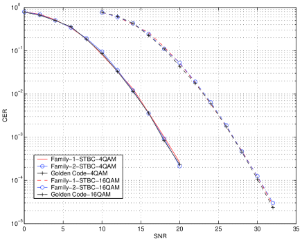
Figure 1: Comparison of the CER of the best $2\times 2$ codes in two fast-decodable STBC families and of the Golden code with $4$- and $16$-QAM signalings.

Let us define the signal-to-noise ratio SNR$\triangleq n_{t}E_{s}/N_{0}$, where $E_{s}$ the average energy. Fig. 1 compares the codeword error rate (CER) of the best STBCs in the two families and of the Golden code with $4$- and $16$-QAM signaling. It is shown that both families of fast-decodable STBCs exhibit similar CER performances, and both differ slightly, at high SNR, from that of Golden code. Since the latter has the best CER known, but does not admit simplified decoding, this small difference can be viewed as the penalty to be paid for complexity reduction.

IV-A Decoding Family-I and II STBCs

By direct computation, we have $\langle\mathbf{f}_{2},\mathbf{e}_{1}\rangle=0$ and $\langle\mathbf{f}_{4},\mathbf{e}_{3}\rangle=0$. In fact we can see that the full-rate fast-decodable STBCs are obtained by linearly combining two rate-1 codes: ${\mathbf{X}}_{1,2}$ and ${\mathbf{X}}_{3,4}$. Moreover, by examining the structures of the $2\times 2$ STBCs and the matrix $\mathbf{R}$, we obtain the results that follow:

Proposition 1

We have $\langle\mathbf{f}_{2},\mathbf{e}_{1}\rangle=0$ if and only if $\mathbf{X}_{1,2}$ is an Alamouti STBC. Consequently, the fast-decodable full-rate $2\times 2$ STBCs only exist for $k^{\prime}=2$ and their corresponding worst-case decoding complexity does not exceed $2M^{3}$. $\hfill\square$

Proof: First, if $\mathbf{X}_{1,2}$ is an Alamouti STBC, from (20) we conclude that $\langle\mathbf{f}_{2},\mathbf{f}_{1}\rangle=0$, and therefore

$$\langle\mathbf{f}_{2},\mathbf{e}_{1}\rangle=\langle\mathbf{f}_{2},\frac{\mathbf{f}_{1}}{\|\mathbf{f}_{1}\|}\rangle=0$$

Second, since ${\mathbf{X}}_{1,2}$ is a rate-1 STBC, it was shown in [17, Theorem 5.4.2] that complex linear-processing orthogonal designs only exist in $2$ dimensions and the Alamouti scheme is unique. Thus, 1) the orthogonality condition $\langle\mathbf{f}_{2},\mathbf{e}_{1}\rangle=0$ in $2\times 2$ STBCs implies that ${\mathbf{X}}_{1,2}$ must have an Alamouti structure, which completes the proof of the converse implication; and 2) this also implies that it is only possible to have $\langle{\mathbf{f}}_{2},{\mathbf{e}}_{1}\rangle=0$ for the fast-decodable full-rate $2\times 2$ STBCs. Based on Definition 6, it yields $k^{\prime}=2$ and the worst-case decoding complexity of $2M^{3}$. $\hfill\square$

To further save computational complexity, we may require $\langle\mathbf{f}_{4},\mathbf{e}_{3}\rangle=0$. This can be obtained if both $\mathbf{X}_{1,2}$ and $\mathbf{X}_{3,4}$ have the Alamouti structure. Note that this condition is sufficient but not necessary, since the Alamouti structure implies $\langle\mathbf{f}_{4},\mathbf{e}_{3}\rangle=0$, but the converse is not true.

The Alamouti structure of $\mathbf{X}_{1,2}$ and $\mathbf{X}_{3,4}$ yields some zero entries in matrix $\mathbf{R}$ and we have the following:

Proposition 2

The other elements in the matrix $\bf R$ cannot be nulled. $\square$

Proof: By direct computation we easily verify $\langle\mathbf{f}_{i},\mathbf{f}_{j}\rangle\neq 0$, $i\in[1,2]$, $j\in[3,4]$. Therefore this code is not an orthogonal STBC [17], and we have

$$\langle\mathbf{f}_{3},\mathbf{e}_{1}\rangle=\langle\mathbf{f}_{3},\frac{\mathbf{f}_{1}}{\|\mathbf{f}_{1}\|}\rangle\neq 0~{}~{}~{}~{}\text{and}~{}~{}~{}~{}\langle\mathbf{f}_{4},\mathbf{e}_{1}\rangle\neq 0$$ (32)

With $\langle{\mathbf{f}}_{2},{\mathbf{e}}_{1}\rangle=0$, we have

$$\mathbf{e}_{2}=\frac{\mathbf{f}_{2}-{\rm Proj}_{\mathbf{e}_{1}}\mathbf{f}_{2}}{\|\mathbf{f}_{2}-{\rm Proj}_{\mathbf{e}_{1}}\mathbf{f}_{2}\|}=\frac{\mathbf{f}_{2}}{\|\mathbf{f}_{2}\|}$$ (33)

then,

$$\langle\mathbf{f}_{3},\mathbf{e}_{2}\rangle=\langle\mathbf{f}_{3},\frac{\mathbf{f}_{2}}{\|\mathbf{f}_{2}\|}\rangle\neq 0~{}~{}~{}~{}\text{and}~{}~{}~{}~{}\langle\mathbf{f}_{4},\mathbf{e}_{2}\rangle\neq 0$$ (34)

Due to (32) and (34), the corresponding elements in $\mathbf{R}$ cannot be nulled. $\hfill\square$

In summary, a $2\times 2$ STBC of the form (22) has complexity $2M^{3}$ if it satisfies Proposition 1. If in addition ${\mathbf{X}}_{3,4}$ has Alamouti structure, then extra computational savings are available in the SD algorithm. Moreover, if cubic shaping is required, the generator matrix ${\mathbb{G}}$ of the STBC is orthogonal.

V New $4\times 2$ STBC and its decoding complexity

Here we design a fast-decodable full-rate $(R=2)$ $4\times 2$ STBC based on the concepts elaborated upon in the previous sections. Specifically, using the twisted structure described above, we combine linearly two rate-$1$ codes. Since rate-$1$ orthogonal codes do not exists for $4$ transmit antennas, we resort quasi-orthogonal STBCs instead [9].

Definition 7

(Quasi-orthogonal structure) [9]  A code whose words have the form

$$\mathbf{X}=\left[\begin{array}[]{rrrr}s_{1}&-s^{*}_{2}&-s^{*}_{3}&s_{4}\\ s_{2}&s^{*}_{1}&-s^{*}_{4}&-s_{3}\\ s_{3}&-s^{*}_{4}&s^{*}_{1}&-s_{2}\\ s_{4}&s^{*}_{3}&s^{*}_{2}&s_{1}\end{array}\right]$$

or another equivalent form as defined in [9], where $s_{i}\in\mathbb{C}$, $i=1,\ldots,4$, is said to have a quasi-orthogonal structure. The quasi-orthogonal STBC is not full rank and has $r=2$. $\hfill\square$

Definition 8

(Full-rate, fast-decodable STBC for $4\times 2$ MIMO) A full-rate $(R=2)$, fast-decodable STBC for $4\times 2$ MIMO, denoted ${\mathcal{G}}^{\prime}$, has $\kappa=8~{}{\rm symbols/codeword}$, and can be decoded by a $12$-dimensional real SD algorithm (rather than the standard 16-dimensional SD). $\hfill\square$

The $4\times 4$ codeword matrix $\mathbf{X}\in{\mathcal{G}}^{\prime}$ encodes eight QAM symbols $\mathbf{s}=[s_{1},\ldots,s_{8}]\in\mathbb{Z}^{8}[j]$, and is transmitted by using the channel four times, so that $T=4$. We admit the sum structure:

$$\mathbf{X}=\mathbf{X}_{1,2}(s_{1},s_{2},s_{3},s_{4})+\mathbf{X}_{3,4}(s_{5},s_{6},s_{7},s_{8})$$ (35)

where $\mathbf{X}_{1,2}(s_{1},s_{2},s_{3},s_{4})$ is a quasi-orthogonal STBC, and

$$\mathbf{X}_{3,4}(z_{1},z_{2},z_{3},z_{4})\triangleq\mathbf{T}\left[\begin{array}[]{rrrr}z_{1}&-z^{*}_{2}&-z^{*}_{3}&z_{4}\\ z_{2}&z^{*}_{1}&-z^{*}_{4}&-z_{3}\\ z_{3}&-z^{*}_{4}&z^{*}_{1}&-z_{2}\\ z_{4}&z^{*}_{3}&z^{*}_{2}&z_{1}\end{array}\right]$$ (36)

with

$$\mathbf{T}=\left[\begin{array}[]{rrrr}1&0&0&0\\ 0&1&0&0\\ 0&0&-1&0\\ 0&0&0&-1\end{array}\right]$$ (37)

and

$$\left[z_{1},z_{2},z_{3},z_{4}\right]^{T}=\mathbf{U}\left[s_{5},s_{6},s_{7},s_{8}\right]^{T}$$ (38)

where $z_{i}\in\mathbb{C}$, $i=1,\ldots,4$, $s_{k}\in\mathbb{Z}[j]$, $k=5,\ldots,8$, and $\mathbf{U}$ is a $4\times 4$ unitary matrix.

Remark 1

(Rank 2) Since the matrix $\mathbf{X}_{1,2}$ has the quasi-orthogonal structure, the code does not have full rank. In particular, it has $r=2$. $\hfill\square$

Remark 2

(Cubic shaping) Direct computation shows that the matrix $\mathbf{T}$ guarantees cubic shaping. $\hfill\square$

We conduct a search over the matrices $\mathbf{U}$, leading to the minimum of $\sum_{\delta}A(2,\delta)$, where the terms $A(2,\delta)$ represent the total number of pairwise error events of rank $2$ and product distance $\delta$. Since an exhaustive search through all $4\times 4$ unitary matrices is too complex, we focus on those with the form

$$\mathbf{U}=\mathbf{D}\mathbf{P}$$ (39)

where $\mathbf{P}\triangleq[\exp(j2\pi\ell n/4)]$ is a $4\times 4$ discrete Fourier transform matrix, $\mathbf{D}={\rm diag}(\exp(j2\pi n_{\ell}/N))$ for some integer $N$, and $n_{\ell}\in\{0,1,\ldots,N\}$ for $\ell=1,\ldots,4$.

For $4$-QAM signaling, taking $N=7$ and $n_{\ell}=1,2,5,6$, we have obtained

$$\tiny\mathbf{U}=\left[\begin{array}[]{rrrr}0.31+0.39i&0.31+0.39i&0.31+0.39i&0.31+0.39i\\ -0.11+0.49i&-0.49-0.11i&0.11-0.49i&0.49+0.11i\\ -0.11-0.49i&0.11+0.49i&-0.11-0.49i&0.11+0.49i\\ 0.31-0.39i&-0.39-0.31i&-0.31+0.39i&0.39+0.31i\end{array}\right]$$

which yields the minimum $\sum_{\delta}A(2,\delta)$.

Under $4$-QAM signaling, we compare the minimum determinants $\delta_{min}$ and their associated multiplicities $A(r,\delta_{min})$, as well as the CERs of the above STBC to the following $4\times 2$ codes:

1. Code with the structure (35), with $\mathbf{U}$ the $4\times 4$ “perfect” rotation matrix [11].

2. The best DjABBA code of [7].

3. The “perfect” two-layer code of [6].

Determinant and multiplicity values are shown in Table II. It can be seen that the proposed $4\times 2$ STBC has the smallest $\sum A(2,\delta)$, when compared to the rank-2 code with perfect rotation matrix $\mathbf{U}$ in  [11]. The CERs are shown in Fig. 2. The proposed code achieves the best CER up to the CER of $10^{-5}$. Due to the diversity loss, the performance curves of the new code and the one of DjABBA cross over at CER of $2\times 10^{-5}$.

For 16-QAM signaling, the best matrix $\mathbf{U}$ with $N=17$ and $n_{\ell}=3,4,5,13$ is

$$\tiny\mathbf{U}=\left[\begin{array}[]{rrrr}0.22+0.44j&0.22+0.44j&0.22+0.44j&0.22+0.44j\\ 0.05+0.50j&-0.49+0.05j&-0.05-0.50&0.50-0.05j\\ -0.30-0.40j&0.30+0.40j&-0.30-0.40j&0.30+0.40j\\ 0.05-0.50j&-0.50-0.05j&-0.05+0.50j&0.50+0.05j\end{array}\right]$$

The performance of this code is compared with that of other codes in Fig. 2. We can see that, at CER$=10^{-4}$, it requires an SNR $0.4$ dB higher than the best known code of [7], which was not designed for reduced-complexity decoding.

Finally, we notice that the first two colums of ${\mathbf{X}}_{1,2}$ are two stacked Alamouti blocks. This provides the orthogonality condition $\langle{\mathbf{f}}_{2},{\mathbf{e}}_{1}\rangle=0$. Therefore the worst-case decoding complexity of fast-decodable $4\times 2$ STBCs is $2M^{7}$, as compared to a standard SD complexity $M^{8}$.

VI Conclusion

We have derived conditions for reduced-complexity ML decoding, and applied them to a unified analysis of two families of full-rate full-diversity $2\times 2$ STBCs that were recently proposed. Moreover, we have compared their minimum determinant, CER performance, and shaping property, and examined how both families allow low-complexity ML decoding. We have also introduced design criteria of fast-decodable STBCs for $2\times 2$ MIMO. These design criteria were finally extended to the construction of a fast-decodable $4\times 2$ code. By combining algebraic and quasi-orthogonal STBC structures, a new code was found that outperforms any known $4\times 2$ code for $4$-QAM signaling, yet with a decoding complexity of $2M^{7}$ in lieu of the worst-case ML decoding complexity $M^{8}$.

${\mathcal{G}}$	$\delta_{\min}$, 4-QAM	$\delta_{\min}$, 16-QAM	$\delta_{\min}$, 64-QAM
1st Family	2.2857	2.2857	2.2857
2nd Family	1.9973	1.9796	1.8784
Golden Code	3.2	3.2	3.2

TABLE I: The minimum determinants $\delta_{\min}$ of the Golden code and two families of fast-decodable STBCs with $4$-, $16$-, and $64$-QAM signaling.

Codes	$\delta_{\rm min}$	Multiplicities
New STBC	$0$	$\sum_{\delta}A(2,\delta)=160$
Perfect Code $\mathbf{U}$ matrix	$0$	$\sum_{\delta}A(2,\delta)=560$
DjABBA	$0.8304$	$A(4,0.8304)=770$
Two-Layers Perfect Code	$0.0016$	$A(4,0.0016)=128$

TABLE II: Minimum determinants of $4\times 2$ STBCs with $4$-QAM signaling

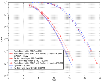
Figure 2: Comparison of the CER of different $4\times 2$ STBCs with 4-QAM signaling.

References

- [1] S. M. Alamouti, “A simple transmit diversity technique for wireless communications,” IEEE J. Select. Areas Commun., vol. 16, no. 8, pp. 1451–1458, October 1998.
- [2] J.-C. Belfiore, G. Rekaya, and E. Viterbo, “The Golden Code: A full-rate space–time code with non-vanishing determinants,” IEEE Trans. Inform. Theory, vol. 51, no. 4, pp. 1432–1436, April 2005.
- [3] M.O. Damen, A. Chkeif, and J.-C. Belfiore, “Lattice code decoder for space–time codes,” IEEE Communication Letters, vol. 4, no. 5, pp. 161–163, May 2000.
- [4] M.O. Damen, H. El Gamal, and G. Caire, “On maximum-likelihood detection and the search for the closest lattice point,” IEEE Trans. Inform. Theory, vol. 49, no. 10, pp. 2389–2402, October 2003.
- [5] J.-C. Guey, M.P. Fitz, M.R. Bell, and W.-Y. Guo, “Signal design for transmitter diversity wireless communication Systems over Ranleith fading channels,” IEEE Trans. Commun., vol. 47, no. 4, pp. 527–537, 1999.
- [6] Y. Hong, E. Viterbo, and J.-C. Belfiore, “A space–time block coded multiuser MIMO downlink transmission scheme,” in Proc. IEEE Int. Symp. Inform. Theory (ISIT 2006), pp. 257–261, Seattle, WA, USA, June–July, 2006.
- [7] A. Hottinen and O. Tirkkonen, “Precoder designs for high rate space–time block codes,” in Proc. Conference on Information Sciences and Systems, Princeton, NJ, March 17–19, 2004.
- [8] A. Hottinen, O. Tirkkonen and R. Wichman, Multi-Antenna Transceiver Techniques for 3G and Beyond. Chichester, UK: John Wiley & Sons Ltd., 2003.
- [9] H. Jafarkhani, “A quasi-orthogonal space–time block code,” in IEEE Commun. Letters, vol. 49, no. 1, pp. 1–4, January 2001.
- [10] E. G. Larsson and P. Stoica, Space-Time Block Coding for Wireless Communications. Cambridge, UK: Cambridge University Press, 2003.
- [11] F. Oggier, G. Rekaya, J.-C. Belfiore, and E. Viterbo, “Perfect space–time block codes,” IEEE Trans. Inform. Theory, vol. 52, n. 9, pp. 3885–3902, September 2006.
- [12] F. Oggier, J-C. Belfiore, and E. Viterbo, “Cyclic Division Algebras: A Tool for Space-Time Coding,” Foundations and Trends in Communications and Information Theory, vol. 4, No. 1, pp. 1-95, 2007.
- [13] J. Paredes, A.B. Gershman, and M. G. Alkhanari, “A space–time code with non-vanishing determinants and fast maximum likelihood decoding,” in Proc IEEE International Conference on Acoustics, Speech, and Signal Processing (ICASSP 2007), Honolulu, Hawaii, USA, pp. 877–880, April 2007.
- [14] M. Samuel and M. P. Fitz, “Reducing the detection complexity by using 2 2 multi-strata space–time codes,” in Proc IEEE Int. Symp. Inform. Theory (ISIT 2007), pp. 1946–1950, Nice, France, June 2007.
- [15] C. P. Schnorr and M. Euchner, “Lattice basis reduction: Improved practical algorithms and solving subset sum problems,” Math Programming, vol. 66, pp. 181–191, 1994.
- [16] S. Sezginer and H. Sari, “A full-rate full-diversity space–time code for mobile WiMAX Systems,” in Proc. IEEE International Conference on Signal Processing and Communications, Dubai, July 2007.
- [17] V. Tarokh, H. Jafarkhani, A. R. Calderbank, “Space–time block codes from orthogonal designs,” IEEE Trans. Inform. Theory, vol. 45, no. 5, pp. 1456–1467, July 1999.
- [18] V. Tarokh, N. Seshadri and A. R. Calderbank, “Space–time codes for high data rate wireless communications: performance criterion and code construction,” IEEE Trans. Inform. Theory, vol. 44, no. 2, pp. 744–765, March 1998.
- [19] O. Tirkkonen and A. Hottinen, “Square-matrix embeddable space–time block codes for complex signal constellations,” in IEEE Trans. Inform. Theory, vol. 48, no. 2, , pp. 384–395, February 2002.
- [20] O. Tirkkonen and R. Kashaev, “Combined information and performance optimization of linear MIMO modulations,” in Proc IEEE Int. Symp. Inform. Theory (ISIT 2002), Lausanne, Switzerland, p. 76, June 2002.
- [21] E. Viterbo and E. Biglieri, “A universal lattice decoder,” in GRETSI 14-em̀e Colloque, Juan-les-Pins, France, September 1993.
- [22] E. Viterbo and J. Boutros, “A universal lattice code decoder for fading chanel,” IEEE Trans. Inform. Theory, vol. 45, pp. 1639–1642, July 1999.