Diagnosing GRB Prompt Emission Site with Spectral Cut-Off Energy

Abstract

The site and mechanism of gamma-ray burst (GRB) prompt emission is still unknown. Although internal shocks have been widely discussed as the emission site of GRBs, evidence supporting other emission sites, including the closer-in photosphere where the fireball becomes transparent and further-out radii near the fireball deceleration radius where magnetic dissipation may be important, have been also suggested recently. With the successful operation of the GLAST experiment, prompt high energy emission spectra from many GRBs would be detected in the near future. We suggest that the cut-off energy of the prompt emission spectrum from a GRB depends on both the fireball bulk Lorentz factor and the unknown emission radius from the central engine. If the bulk Lorentz factor could be independently measured (e.g. from early afterglow observations), the observed spectral cutoff energy can be used to diagnose the emission site of gamma-rays. This would provide valuable information to understand the physical origin of GRB promp emission.

1 Introduction

The emission of photons in the prompt phase of a GRB may last from less than a second to hundreds of seconds (see e.g. Mészáros (2006) for a recent general review on GRBs). The exact physical mechanism and the emission site of the observed prompt GRB emissions are still unknown (Zhang & Mészáros, 2004; Zhang, 2007). The physical processes which may lead to this emission include synchrotron/jitter emission, inverse Compton scattering or a combination of thermal and non-thermal emission components. Internal shocks have been widely discussed in the literature as the possible emission site of GRB prompt emission (Rees & Mészáros 1994; Mészáros et al. 1994; Kobayashi et al. 1997; Daigne & Mochkovitch 1998; Pilla & Loeb 1998; Panaitescu & Mészáros 2000; Lloyd & Petrosian 2000; Zhang & Mészáros 2002a; Dai & Lu 2002; Pe’er & Waxman 2004, 2005; Pe’er et al. 2005; Gupta & Zhang 2007). Within this model the radius of emission from the central engine ($r$) is related to the bulk Lorentz factor ($\Gamma$) and the variability time ($t_{v}$) through $r=\Gamma^{2}ct_{v}$. For typically observed values of bulk Lorentz factor $\Gamma\sim 300$ and variability time $t_{v}\sim 0.01~{}$sec the emission radius is $r\sim 3\times 10^{13}~{}$cm. However, the internal shock origin of GRB prompt emission is not conclusive. The baryonic or pair photospheres of the GRB fireball have been argued to be another possible emission site of prompt GRB emission (e.g. Thompson 1994; Mészáros & Rees 2000; Mészáros et al. 2002; Ryde 2005). This model has the merit of potentially reproducing some observed empirical correlations among GRB prompt emission properties (e.g. Rees & Mészáros 2005; Ryde et al. 2006; Thompson et al. 2007; cf. Zhang & Mészáros 2002). On the other hand, an analysis of Swift early afterglow data led Kumar et al. (2007) to conclude that the prompt emission site is between $10^{15}$-$10^{16}$cm from the central engine. This emission site is too large for typical internal shocks but too small for external shocks. Emission at this radius may be related to magnetic dissipation (e.g. Spruit et al. 2001; Drenkhahn & Spruit 2002; Zhang & Mészáros 2002; Giannios & Spruit 2007). In both of the above two non-internal shock models for GRB prompt emissions, it is possible to argue that the emission radius $r$ could be in principle related to the Lorentz factor $\Gamma$ and variability $t_{v}$ in a non-trivial (e.g. other than $r=\Gamma^{2}ct_{v}$) manner. For example, in the photosphere model, $r$ is defined by the optically-thin condition, and is not directly related to $t_{v}$ which is related to the time history of the GRB central engine. In the magnetic dissipation model, if the energy dissipation occurs locally (i.e. the emission region scale is much smaller than the emission radius), it is possible to have $r>\Gamma^{2}ct_{v}$. In general, it is reasonable to treat $r$ as an independent quantity with respect to $\Gamma$ and $t_{v}$.

High energy photons produced in the prompt emission region are expected to interact with lower energy photons before escaping as a result of two photon attenuation. In general, the internal optical depth of $\gamma\gamma$ interactions depends on $\Gamma$, $t_{v}$, and the radius of the emission region. Traditionally, internal shocks have been taken as the default model of GRB prompt emission, and the pair attenuation optical depth has been expressed as a function of $\Gamma$ and $t_{v}$ only (e.g. Piran 1999; Lithwick & Sari 2001). The pair attenuation process is expected to leave a cutoff spectral feature in the prompt emission spectrum, and detecting such a spectral cutoff by high energy missions such as GLAST has been discussed as an important method to estimate the bulk Lorentz factor $\Gamma$ of the fireball (Baring & Harding, 1997; Baring, 2006). The issue of unknown emission radius $r$ makes the picture more complicated. It is no longer straightforward to estimate $\Gamma$ with an observed spectral cutoff energy. On the other hand, there are other independent methods of estimating $\Gamma$ using early afterglow (e.g. Sari & Piran 1999; Zhang, Kobayashi & Mészáros 2003) or prompt emission (Pe’er et al. 2007) data and there have been cases of such measurements (Molinari et al. 2007; Pe’er et al. 2007). It is then possible to use the observed spectral cutoff energy to diagnose the unknown GRB emission site if $\Gamma$ is measured by other means. In this paper we release the internal shock assumption and re-express the cutoff energy more generally as a function of $r$ and $\Gamma$. We then discuss an approach of diagnosing the GRB prompt emission site using the future cutoff energy data retrieved by GLAST and other missions. Lately Murase & Ioka (2007, see also Murase & Nagataki 2006) also independently discussed to use the pair cutoff signature to diagnose whether the emission site is the pair/baryonic photosphere. We discuss this topic more generally to diagnose any emission site. We emphasise that our method can be used to constrain $r$ only when a clear cut-off is observed in the high energy photon spectrum from a GRB.

2 Parametrization of Internal Optical Depth

The cross section of two-photon interaction can be generally expressed as (Gould & Schreder 1967)

$$\sigma_{\gamma_{h}\gamma_{l}}(E_{\gamma_{h}}^{\prime},E_{\gamma_{l}}^{\prime},\theta^{\prime})=\frac{3}{16}\sigma_{T}(1-{b}^{2})\Big{[}(3-{b}^{4})\ln{\frac{1+{b}}{1-{b}}}-2{b}(2-{b}^{2})\Big{]}~{},$$ (1)

where $\sigma_{T}$ is the Thomson cross section, $b=[1-(E_{\gamma_{l},th}^{\prime}/E_{\gamma_{l}}^{\prime})]^{1/2}$ is the center of mass dimensionless speed of the pair produced, $E_{\gamma h}^{{}^{\prime}}$, $E_{\gamma l}^{{}^{\prime}}$ and $\theta^{\prime}$ are the high- and low-energy photon energies and their incident angles in the comoving frame of the GRB ejecta. The threshold energy of pair production for a high energy photon with energy $E_{\gamma_{h}}^{\prime}$ is

$$E_{\gamma_{l},th}^{\prime}=\frac{2(m_{e}c^{2})^{2}}{E_{\gamma_{h}}^{\prime}(1-\cos{\theta^{\prime}})}~{}.$$ (2)

In the comoving frame, the relative velocity of the high energy and low energy photons along the direction of the former is $c(1-\cos{\theta^{\prime}})$. For an isotropic distribution the fraction of low energy photons moving in the differential cone at an angle between $\theta^{\prime}$ and $(\theta^{\prime}+d\theta^{\prime})$ is $\frac{1}{2}\sin\theta^{\prime}d{\theta^{\prime}}$. The inverse of the mean free path for $\gamma_{h}$ $\gamma_{l}$ interactions $l_{\gamma_{h}\gamma_{l}}^{-1}(E_{\gamma_{h}}^{\prime})$ can be calculated as

$$l_{\gamma_{h}\gamma_{l}}^{-1}(E_{\gamma_{h}}^{\prime})=\frac{1}{2}\int_{-1}^{+1}d(\cos{\theta^{\prime}})(1-\cos{\theta^{\prime}})l_{\gamma_{h}\gamma_{l}\theta^{\prime}}^{-1}(E_{\gamma_{h}}^{\prime},\theta^{\prime})$$ (3)

where

$$l_{\gamma_{h}\gamma_{l}\theta^{\prime}}^{-1}(E_{\gamma_{h}}^{\prime},\theta^{\prime})=\int_{E_{\gamma_{l},th}^{\prime}}^{\infty}d{E_{\gamma_{l}}^{\prime}}\frac{dn_{\gamma_{l}}(E_{\gamma_{l}}^{\prime})}{d{E_{\gamma_{l}}^{\prime}}}\sigma_{\gamma_{h}\gamma_{l}}(E_{\gamma_{h}}^{\prime},E_{\gamma_{l}}^{\prime},\theta^{\prime})~{},$$ (4)

$\frac{dn_{\gamma_{l}}(E_{\gamma_{l}}^{\prime})}{dE_{\gamma_{l}}^{\prime}}$ is the specific number density of low energy photons of the GRB in the comoving frame. The observed low energy photon spectrum (per unit energy per unit area) $\frac{dN_{\gamma_{l}}^{\rm o}(E_{\gamma_{l}}^{\rm o})}{dE_{\gamma_{l}}^{\rm o}dA}$ from a GRB pulse can be used to estimate $\frac{dn_{\gamma_{l}}(E_{\gamma_{l}}^{\prime})}{dE_{\gamma_{l}}^{\prime}}$, i.e.

$$\frac{dn_{\gamma_{l}}(E^{\prime}_{\gamma_{l}})}{dE^{\prime}_{\gamma_{l}}}=\frac{d_{z}^{2}}{r^{2}\Delta^{\prime}}\frac{dN_{\gamma_{l}}^{\rm o}(E_{\gamma_{l}}^{\rm o})}{dE_{\gamma_{l}}^{\rm o}dA}\frac{dE_{\gamma_{l}}^{\rm o}}{dE^{\prime}_{\gamma_{l}}}$$ (5)

where $\Delta^{\prime}$ is the comoving width of the shell at the radius $r$ from the central engine. We notice that the expression of $\Delta^{\prime}$ is function of radius (e.g. Zhang & Mészáros 2002b): $\Delta^{\prime}=r$ for $r<r_{c}$; $\Delta^{\prime}=r_{c}=\Gamma ct_{v}$ for $r_{c}\leq r<r_{s}$; and $\Delta^{\prime}=r/\Gamma$ for $r\geq r_{s}=\Gamma^{2}ct_{v}$. Throughout the paper the superscript “o” denotes the quantities measured in the observer’s rest frame.

The comoving distance of the source is

$$d_{z}=\frac{c}{H_{0}}\int_{0}^{z}\frac{dx}{\sqrt{\Omega_{\Lambda}+\Omega_{m}(1+x)^{3}}}~{},$$ (6)

which is related to the luminosity distance through $d_{L}=d_{z}(1+z)$, where $z$ is the redshift of the source. Here $H_{0}=71{\rm km~{}s^{-1}~{}Mpc^{-1}}$ $\Omega_{\Lambda}=0.73$ and $\Omega_{m}=0.27$ are adopted in our calculations. The observed fluence is usually a broken power law with a break energy of the order of MeV (Band et al. 1993). We assume that the two spectral indices below and above the break energy are $-\beta_{1}$ and $-\beta_{2}$, respectively, usually with $\beta_{1}\sim 1$ and $\beta_{2}\geq 2$. We model the observed photon flux as

$$\frac{dN_{\gamma_{l}}^{\rm o}(E_{\gamma_{l}}^{\rm o})}{dE_{\gamma_{l}}^{\rm o}dA}=f^{\rm o}\left\{\begin{array}[]{l@{\quad\quad}l}{E_{\gamma_{l}}^{\rm o}}^{-\beta_{1}}&E_{\gamma_{l}}^{\rm o}<E_{\gamma,br}^{\rm o}\\ {E_{\gamma,br}^{\rm o}}^{\beta_{2}-\beta_{1}}{E_{\gamma_{l}}^{\rm o}}^{-\beta_{2}}&E_{\gamma_{l}}^{\rm o}>E_{\gamma,br}^{\rm o}\end{array}\right.$$ (7)

The break energy in the photon spectrum in the observer’s frame is denoted by $E_{\gamma,br}^{\rm o}$. We define a new variable following the procedure discussed in Gould and Schreder (1967) to reduce the number of integrals

$$s=\frac{E_{\gamma_{l}}^{\prime}E_{\gamma_{h}}^{\prime}(1-\cos{\theta^{\prime}})}{2(m_{e}c^{2})^{2}}=\frac{E_{\gamma_{l}}^{\prime}}{E_{\gamma_{l},th}^{\prime}}=s_{0}\Theta$$ (8)

with $s_{0}=\frac{E_{\gamma_{l}}^{\prime}E_{\gamma_{h}}^{\prime}}{(m_{e}c^{2})^{2}}$, and $\Theta=\frac{1}{2}(1-\cos{\theta^{\prime}})$. As $b=(1-1/s)^{1/2}$, the pair production cross section can be expressed as a function of $s$. It is then possible to write Eq.(3) as

$$l_{\gamma_{h}\gamma_{l}}^{-1}(E_{\gamma_{h}}^{\prime})=\frac{3}{8}\sigma_{T}\Big{(}\frac{m_{e}^{2}c^{4}}{E_{\gamma_{h}}^{\prime}}\Big{)}^{2}\int_{\frac{m_{e}^{2}c^{4}}{E_{\gamma_{h}}^{\prime}}}^{\infty}{E_{\gamma_{l}}^{\prime}}^{-2}\frac{dn_{\gamma_{l}}(E_{\gamma_{l}}^{\prime})}{dE_{\gamma_{l}}^{\prime}}Q[{s_{0}(E_{\gamma_{l}}^{\prime})}]dE^{\prime}_{\gamma l}$$ (9)

where

$$Q[s_{0}(E_{\gamma_{l}}^{\prime})]=\int_{1}^{s_{0}(E_{\gamma_{l}}^{\prime})}s\sigma(s)ds~{},$$ (10)

and $\sigma(s)=\frac{16}{3}\frac{\sigma_{\gamma_{h}\gamma_{l}}}{\sigma_{T}}$. For moderate values of $s$ we use $\sigma(s)\simeq 1$ and the expressions for $Q[s_{0}(E_{\gamma_{l}}^{\prime})]$ becomes $(s_{0}^{2}-1)/2$. Substituting for $Q[s_{0}(E_{\gamma_{l}}^{\prime})]$ in Eq.(9) we derive the final expression for $l_{\gamma_{h}\gamma_{l}}^{-1}(E_{\gamma_{h}}^{\prime})$. Finally, the internal optical depth $\tau_{int}(E_{\gamma_{h}}^{\rm o})$ is the ratio of width of $\gamma_{h}\gamma_{l}$ interaction region and the mean free path of their interaction. In most cases, this is simply

$$\tau_{int}(E_{\gamma_{h}}^{\rm o})=\triangle^{\prime}/l_{\gamma_{h}\gamma_{l}}(E_{\gamma_{h}}^{\rm o})~{}.$$ (11)

In this case, comparing Eqs.(5) and (11) suggests that the concrete expression of $\Delta^{\prime}$ does not enter the problem since it is cancelled out in the expression of $\tau_{int}(E_{\gamma_{h}}^{\rm o})$. In the photosphere models that invoke a continous wind from the central engine (Mészáros & Rees, 2000; Giannios, 2006), however, this expression should be modified as

$$\tau_{int}(E_{\gamma_{h}}^{\rm o})=r/[\Gamma l_{\gamma_{h}\gamma_{l}}(E_{\gamma_{h}}^{\rm o})]~{}.$$ (12)

We therefore also consider such a case.

In the following we discuss three cases. The analytical expressions below are only valid for Eq.(11). For the case of continuous photosphere models (Eq.[12]), the analytical expressions for $r<r_{is}$ are more complicated, and we only present the numerical results in Fig.1, where $\Delta^{\prime}=\Gamma ct_{v}$ is used.
Case (I): Both the cutoff energy $E_{\gamma c}^{\rm o}$ (defined by $\tau_{int}(E_{\gamma_{c}}^{\rm o})=1$ at which energy the observed spectrum significantly deviates from the power-law extension of the low energy spectrum) and the threshold energy $E_{\gamma_{l},th}^{\rm o}$ (for $E_{\gamma c}^{\rm o}$) are above the break energy in the observed photon spectrum $E_{\gamma,br}^{\rm o}$, i.e. $E_{\gamma,br}^{\rm o}<E_{\gamma_{l},th}^{\rm o}<E_{\gamma_{c}}^{\rm o}$ (or $E_{\gamma,br}^{\prime}<E_{\gamma_{l},th}^{\prime}<E_{\gamma_{c}}^{\prime}$). The expression for the optical depth is the simplest for this case

$$\tau_{int}(E_{\gamma_{h}}^{\rm o})=\frac{A_{1}(E_{\gamma_{h}}^{\rm o})}{r^{2}}\Big{(}\frac{\Gamma}{1+z}\Big{)}^{2-2\beta_{2}}$$ (13)

where

$$A_{1}(E_{\gamma_{h}}^{\rm o})=\frac{3\sigma_{T}{d_{z}}^{2}f^{\rm o}_{1}}{8({\beta_{2}}^{2}-1)}\Big{(}\frac{E_{\gamma_{h}}^{\rm o}}{{m_{e}}^{2}c^{4}}\Big{)}^{\beta_{2}-1}$$ (14)

and $\frac{dN_{\gamma_{l}}^{\rm o}(E_{\gamma_{l}}^{\rm o})}{dE_{\gamma_{l}}^{\rm o}dA}=f^{\rm o}_{1}{E_{\gamma_{l}}^{\rm o}}^{-\beta_{2}}$ with $f^{\rm o}_{1}=f^{\rm o}{E_{\gamma,br}^{\rm o}}^{\beta_{2}-\beta_{1}}$ has been assumed for $E_{\gamma_{l}}^{\rm o}>E_{\gamma,br}^{\rm o}$. In the case of internal shocks the radius of prompt emission is $r=\Gamma^{2}ct_{v}^{\rm o}/(1+z)$ where $t_{v}^{\rm o}$ is the observed variability time scale. Substituting this expression of $r$ in Eq.(13) one gets $\tau_{int}(E_{\gamma_{h}}^{\rm o})\propto\Gamma^{-2-2\beta_{2}}$, which is consistent with Lithwick & Sari (2001). Our expression is more generic with $r$ being a free parameter.
Case (II): If the cutoff energy is still above the break energy, but the threshold energy for pair production is below the break energy, i.e. ($E_{\gamma_{l},th}^{\rm o}<E_{\gamma,br}^{\rm o}<E_{\gamma_{c}}^{\rm o}$), the expression for internal optical depth is more complicated. Making use of Eq.(7), one gets

$$\tau_{int}(E_{\gamma_{h}}^{\rm o})=\frac{A_{2}(E_{\gamma_{h}}^{\rm o})}{r^{2}}\Big{(}\frac{\Gamma}{1+z}\Big{)}^{2-2\beta_{1}}$$ (15)

with

$$A_{2}(E_{\gamma_{h}}^{\rm o})=\frac{3\sigma_{T}{d_{z}}^{2}f^{\rm o}}{16}\Big{(}\frac{{m_{e}}^{2}c^{4}}{E_{\gamma_{h}}^{\rm o}}\Big{)}^{2}\Big{[}\Big{(}\frac{E_{\gamma_{h}}^{\rm o}}{{m_{e}}^{2}c^{4}}\Big{)}^{2}\Big{(}\frac{E_{\gamma_{h},br}^{\rm o}}{{m_{e}}^{2}c^{4}}\Big{)}^{\beta_{1}-1}\Big{(}\frac{\beta_{1}-\beta_{2}}{(\beta_{2}-1)(\beta_{1}-1)}\Big{)}$$

$$+{\Big{(}\frac{E_{\gamma_{h},br}^{\rm o}}{{m_{e}}^{2}c^{4}}\Big{)}^{1+\beta_{1}}}\frac{\beta_{2}-\beta_{1}}{(1+\beta_{2})(1+\beta_{1})}+\Big{(}\frac{E_{\gamma_{h}}^{\rm o}}{{m_{e}}^{2}c^{4}}\Big{)}^{1+\beta_{1}}\frac{2}{{\beta_{1}}^{2}-1}\Big{]}$$ (16)

for $\beta_{1}\neq 1$, where $E_{\gamma_{h},br}^{\rm o}$ is the energy of the high energy photons that interact with the break-energy photons at the threshold condition, which is defined by $E_{\gamma_{h},br}^{\rm o}E_{\gamma,br}^{\rm o}=\Big{(}\frac{\Gamma}{1+z}\Big{)}^{2}{m_{e}}^{2}c^{4}$. Equation (16) can be reduced to Eq.(14) when $\beta_{1}=\beta_{2}$. For $\beta_{1}=1$, $\tau_{int}$ does not depend on $\Gamma$, and one has

$$\tau_{int}(E_{\gamma_{h}}^{\rm o})=\frac{3\sigma_{T}f^{\rm o}}{16}\Big{(}\frac{d_{z}}{r}\Big{)}^{2}\Big{(}\frac{{m_{e}}^{2}c^{4}}{E_{\gamma_{h}}^{\rm o}}\Big{)}^{2}\Big{[}\Big{(}\frac{E_{\gamma_{h}}^{\rm o}}{{m_{e}}^{2}c^{4}}\Big{)}^{2}\Big{[}\ln\Big{(}\frac{E_{\gamma_{h}}^{\rm o}}{E_{\gamma_{h},br}^{\rm o}}\Big{)}+\frac{1}{\beta_{2}-1}\Big{]}+\Big{(}\frac{E_{\gamma_{h},br}^{\rm o}}{{m_{e}}^{2}c^{4}}\Big{)}^{2}\Big{[}\frac{1}{2}-\frac{1}{1+\beta_{2}}\Big{]}-\frac{1}{2}\Big{(}\frac{E_{\gamma_{h}}^{\rm o}}{{m_{e}}^{2}c^{4}}\Big{)}^{2}\Big{]}~{}.$$ (17)

In this case $\Gamma$ is not needed to infer $r$.
Case (III): In more extreme cases, usually with a low enough Lorentz factor, one could have the cutoff energy below the break energy, i.e. $E_{\gamma_{l},th}^{\rm o}<E_{\gamma_{c}}^{\rm o}<E_{\gamma,br}^{\rm o}$.

In this regime, we still use Eq.(9) to calculate the internal optical depth, but effectively one can place the upper limit of the integration as the break energy, since above the break energy the photon flux falls off rapidly. This gives

$$\tau_{int}(E_{\gamma_{h}}^{\rm o})=\frac{A_{3}(E_{\gamma_{h}}^{\rm o})}{r^{2}}\Big{(}\frac{\Gamma}{1+z}\Big{)}^{2-2\beta_{1}}$$ (18)

where

$$A_{3}(E_{\gamma_{h}}^{\rm o})=\frac{3\sigma_{T}{d_{z}}^{2}f^{\rm o}}{16}\Big{[}\frac{2}{{\beta_{1}}^{2}-1}\Big{(}\frac{E_{\gamma_{h}}^{\rm o}}{{m_{e}}^{2}c^{4}}\Big{)}^{\beta_{1}-1}-\frac{1}{\beta_{1}-1}\Big{(}\frac{E_{\gamma_{h},br}^{\rm o}}{m_{e}^{2}c^{4}}\Big{)}^{\beta_{1}-1}+\frac{1}{1+\beta_{1}}\Big{(}\frac{m_{e}^{2}c^{4}}{E_{\gamma_{h}}^{\rm o}}\Big{)}^{2}\Big{(}\frac{E_{\gamma_{h},br}^{\rm o}}{m_{e}^{2}c^{4}}\Big{)}^{1+\beta_{1}}]$$ (19)

To summarize all three cases, the radius of the prompt emission can be calculated in terms of cutoff energies by making the internal optical depths (Eqs.[13,15,18]) to unity

$$r=[A_{i}(E_{\gamma_{c}}^{\rm o})]^{1/2}\Big{(}\frac{\Gamma}{1+z}\Big{)}^{1-\beta_{j}}$$ (20)

where $j=2$ for $i=1$, and $j=1$ for $i=2,3$. In practice, from the observed low energy photon spectrum it is possible to derive the low energy photon spectral parameters (including $\beta_{1}$, $\beta_{2}$, $E_{\gamma,br}^{\rm o}$, $E_{\gamma_{c}}^{\rm o}$, etc.) and to identify one applicable case among the three cases discussed. If the burst redshift $z$ is measured from afterglow observations, and if the GRB bulk Lorentz factor is measured or constrained independently with other methods (e.g. Zhang et al. 2003; Molinari et al. 2007; Pe’er et al. 2007), one can estimate the GRB emission radius using Eq.(20). For the case (I) and if $\beta_{2}\sim 2$, a very simple expression of $r$ is available according to Eq.(13)

$$r=\frac{d_{L}}{m_{e}c^{2}\Gamma}\Big{(}\frac{\sigma_{T}f^{\rm o}_{1}E_{\gamma_{c}}^{\rm o}}{8}\Big{)}^{1/2}~{}~{}$$ (21)

which could be used to quickly estimate $r$ with the data.

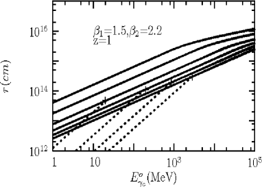
Figure 1: (a) Contours of $E_{\gamma_{c}}^{\rm o}$ in the $r-\Gamma$ plane. From top to bottom, $E_{\gamma_{c}}^{\rm o}=$50GeV, 5GeV, 0.5GeV, 50MeV, 5MeV and 0.5MeV, respectively. Model inputs: $E_{\gamma,br}^{\rm o}=1$MeV, observed flux is $0.6{\rm MeV^{-1}cm^{-2}}$ at $E_{\gamma,br}^{\rm o}$, $z=1$, $\beta_{1}=1.5$ and $\beta_{2}=2.2$. The solid lines are derived from Eq.(11). The dotted lines are derived from Eq.(12) for $r<r_{is}$. The dashed line represents the internal shock $r-\Gamma$ relation, and the variability time $t_{v}=0.01$sec is assumed. (b) Inferring $r$ from the observed cutoff energy. From top to bottom, $\Gamma=100,200,400,600,800$, and 1000, respectively. Other parameters and line styles are the same as (a). The crosses on the lines for $\Gamma=400$ to $1000$ are for the internal shock model with $t_{v}=0.01$sec.

3 Case Study and Discussion

We have generalized the expression of the cutoff energy of prompt GRB spectrum to include the dependences of both $\Gamma$ and $r$. We suggest that the information of this cutoff energy is useful to diagnose the unknown location of gamma-rays. We discuss three cases, and derive a general expression of $r$ (Eq.[20]). In Fig.1(a) we present the contours of $E_{\gamma_{c}}^{\rm o}$ in the $r-\Gamma$ plane (detailed model parameters are listed in the figure caption). It is straightforward to see that $E_{\gamma_{c}}^{\rm o}$ carries the information of both $\Gamma$ and $r$, and unless the internal shock model is assumed, one cannot constrain $\Gamma$ by $E_{\gamma_{c}}^{\rm o}$. Figure 1(b) indicates that by knowing $\Gamma$ from other measurements, one could diagnose $r$ with the $E_{\gamma_{c}}^{\rm o}$ information. GLAST will be launched in early 2008, and LAT on board will be able to measure the pair cutoff signature for many GRBs. With the coordinated observations with Swift and ground-based follow up observations (to obtain $z$ and $\Gamma$ information), one may be able to more precisely diagnose the emission site of gamma-rays, which is so-far subject to debate.

We notice that the maximum observed photon energy ($e_{\rm max}$) mentioned in the paper by Lithwick & Sari (2001) is not the same as the cut-off energy ($E_{\gamma_{c}}^{o}$) discussed in our paper. They discussed the maximum observed energy defined by the detector bandpass and sensitivity, and used that energy to derive the lower limit of $\Gamma$. Within that context, they discussed two possible limits defined by pair attenuation (limit A) and Compton scattering by pairs (limit B), respectively. Here we discuss the physical cutoff energy, so we can infer the actual value (not lower limits) of $\Gamma$ and $r$ (our new addition). By definition, by regarding $E_{\gamma_{c}}^{o}$ as $e_{\rm max}$ in Lithwick & Sari (2001), their $e_{\rm max,an}$ is just $e_{\rm thick}$, and their self-annihilation energy $e_{\rm self,an}$ is always smaller than or at most equal to $e_{\rm max}$ by definition (otherwise photons cannot be attenuated at $e_{\rm max}=E_{\gamma_{c}}^{o}$). As a result, the limit B discussed by Lithwick & Sari (2001) is never relevant in our context.

We have assumed that the photon field is isotropic in the comoving frame. In some models (e.g. Lyutikov & Blandford 2003; Thompson et al. 2007) the emitters are moving fast in the comoving frame of the bulk flow. This will introduce anisotropy of the photon field in the comoving frame. Suppose the relative bulk Lorentz factor of the emitter in the comoving frame is $\Gamma^{\prime}_{e}\sim$ several, the photon interaction angle is at most $2/\Gamma^{\prime}_{e}$. This will reduce the optical depth for pair production. The inferred $r$ (given a same $\Gamma$) should be smaller. For example, for $\Gamma^{\prime}_{e}\sim 2$ the optical depth is lower by a factor of $\sim$16 and the inferred $r$ decreases by a factor of $\sim$4.

A possible pair attenuation exponential cutoff signature may have been observed in the pulse 2 of GRB 060105 with the joint Swift-Konus-Wind data (Godet et al. 2007). The observed cutoff is around 600 keV, and the spectral index before the cutoff is flat: $\beta_{1}=0.67$. The observed photon number flux at 1 MeV is 0.5 ${\rm photons~{}cm^{-2}~{}s^{-1}~{}{MeV}^{-1}}$, and the observed duration of the pulse is about 20sec. A pseudo redshift $z\sim 4$ is inferred, which is consistent with the broad pulse profile in the observed lightcurves. This burst likely belongs to Case (III) discussed above. If the cutoff feature is real and is indeed due to pair attenuation, the requirement that $E_{\gamma_{l},th}^{\rm o}$ should be smaller than $E_{\gamma,c}^{\rm o}$ demands $\Gamma\leq 6$. Using Eq.(18), (19), and (20), with $\beta_{1}=0.67$, one can estimate $r\geq 10^{16}$ cm, which is consistent with the conclusion drawn from analyzing the Swift X-ray data (Kumar et al. 2007). Since the quality of the data is poor, we look forward to the high quality data retrieved by GLAST to finally pin down $r$ in the future.

We thank the anonymous referee for important remarks and Olivier Godet, Kohta Murase, Enrico Ramirez-Ruiz for helpful discussion/comments. This work is supported by NASA under grants NNG06GH62G, NNX07AJ66G and NNX07AJ64G.

References

• Band et al. (1993) Band, D. et al. 1993, ApJ, 413, 281.
• Baring & Harding (1997) Baring M., Harding A., 1997, ApJ, 491, 663.
• Baring (2006) Baring M., 2006, ApJ, 650, 1004.
• Dai & Lu (2002) Dai Z. G., Lu T., 2002, ApJ, 580, 1013.
• Daigne & Mochkovitch (1998) Daigne F., Mochkovitch R., 1998, MNRAS, 296, 275.
• Drenkhahn & Spruit (2002) Drenkhahn G., Spruit H. C., 2002, A&A, 391, 1141.
• Giannios (2006) Giannios, D. 2006, A & A, 457, 763.
• Giannios & Spruit (2007) Giannios, D., Spruit, H. C. 2007, A&A, 469, 1.
• Godet et al. (2007) Godet O. et al., 2007, submitted.
• Gould & Schreder (1967) Gould, R. J., Schreder, G. P. 1967, Phys. Rev. 155, 1404.
• Gupta & Zhang (2007) Gupta N., Zhang B., 2007, MNRAS, 380, 78.
• Kobayashi et al. (1997) Kobayashi, S., Piran, T., Sari, R. 1997, ApJ, 490, 92
• Kumar & Panaitescu (2000) Kumar P., Panaitescu, A. 2000, ApJ, 541, L51.
• Kumar et al. (2007) Kumar P. et al., 2007, MNRAS, 376, 57.
• Liang et al. (2006) Liang, E. et al. 2006, ApJ, 646, 351
• Lithwick & Sari (2001) Lithwick Y., Sari R., 2001, ApJ, 555, 540.
• Lloyd & Petrosian (2000) Lloyd N. M., Petrosian V., 2000, ApJ, 543, 722.
• Lyutikov & Blandford (2003) Lyutikov M., Blandford R., 2003, astro-ph/0312347.
• Mészáros et al. (1994) Mészáros P., Rees M. J., Papathanassiou H., 1994, ApJ, 432, 181.
• Mészáros & Rees (2000) Mészáros P., Rees M. J., 2000, ApJ, 530, 292.
• Mészáros et al. (2002) Mészáros P., Ramirez-Ruiz E., Rees M. J., Zhang B., 2002, ApJ, 578, 812.
• Mészáros (2006) Mészáros P., 2006, Rept. Prog. Phys., 69, 2259.
• Molinari et al. (2007) Molinari E. et al., 2007, A&A, 469, L13
• Murase & Nagataki (2006) Murase, K., Nagataki, S. 2006, Phys. Rev. D, 73, 063002.
• Muras & Ioka (2007) Murase K., Ioka K., 2007, ApJ, submitted (arxiv:0708.1370).
• Panaitescu & Mészáros (2000) Panaitescu A., Mészáros P., 2000, ApJ, 544, L17.
• Pe’er & Waxman (2004, 2005) Pe’er A., Waxman E., 2004, ApJ, 613, 448; 2005, ApJ, 628, 857.
• Pe’er et al. (2005) Pe’er A., Mészáros P., Rees M. J., 2005, ApJ, 635, 476.
• Pe’er et al. (2007) Pe’er A., Ryde F., Wijers R. A. M. J., Mészáros P., Rees M. J., 2007, ApJ, 664, L1.
• Pilla & Loeb (1998) Pilla R. P., Loeb A., 1998, ApJ, 494, L167.
• Rees & Mészáros (1994) Rees M. J., Mészáros P., 1994, ApJ, 430, L93.
• Rees & Mészáros (2005) Rees M. J., Mészáros P., 2005, ApJ, 628, 847.
• Ryde (2005) Ryde F., 2005, ApJ, 625, L95.
• Ryde et al. (2006) Ryde F. et al., 2006, ApJ, 652, 1400.
• Sari & Piran (1999) Sari R., Piran T., 1999, ApJ, 520, 641.
• Spruit et al. (2001) Spruit H. C., Daigne F., Drenkhahn G., 2001, A&A, 369, 694.
• Thompson (1994) Thompson C., 1994, MNRAS, 272, 480.
• Thompson (2007) Thompson C., Mészáros P., Rees M. J., 2007, ApJ, 666, 1012.
• Zhang (2007) Zhang B., 2007, Chin. J. A & A, 7, 1.
• Zhang & Mészáros (2004) Zhang B., Mészáros P., 2004, IJMP A, 19, 2385.
• Zhang & Mészáros (2002a) Zhang B., Mészáros P., 2002a, ApJ, 581, 1236.
• Zhang & Mészáros (2002b) Zhang B., Mészáros P., 2002b, ApJ, 566, 712.
• Zhang et al. (2003) Zhang B., Kobayashi S., Mészáros P., 2003, ApJ, 595, 950.
• Zhang et al. (2006) Zhang B. et al., 2006, ApJ, 642, 354.