Phase effects on synchronization by dynamical relaying in delay-coupled systems

Abstract

Synchronization in an array of mutually coupled systems with a finite time-delay in coupling is studied using Josephson junction as a model system. The sum of the transverse Lyapunov exponents is evaluated as a function of the parameters by linearizing the equation about the synchronization manifold. The dependence of synchronization on damping parameter, coupling constant and time-delay is studied numerically. The change in the dynamics of the system due to time-delay and phase difference between the applied fields is studied. The case where a small frequency detuning between the applied fields is also discussed.

Time-delayed systems are interesting because the dimension of chaotic dynamics can be made arbitrarily large by increasing the time-delay and hence find applications in secure communications. Most of the chaos based communication techniques use synchronization in unidirectional drive response system. A limitation which arises in this case is that messages can be sent only in one direction. Thus for a two way transmission of signals, a bidirectional coupling is required. In this work we deal with an array of three mutually coupled Josephson junctions with a finite time-delay in coupling and study the system dynamics in the presence of an external driving field. The effect of phase difference and a small frequency mismatch between the driving fields on a chaotically synchronized system with time delay is then studied.

I Introduction

The equation for Josephson junction (JJ) when treated within the Stewart-McCumber model is identical to the equation for a driven damped pendulum which has been studied theoretically for several routes to chaoshumier ; braiman . Since the work done by Belykh, Pedersen and Soerensen on chaotic dynamics in Josephson junction (JJ) bel ; bely , a great deal of investigations have been carried out as it is an interesting candidate in the field of non linear dynamics. A detailed review of chaos in JJ can be found in kau . Time-delay has been studied experimentally in JJ transmission lines represented by a sequence of overdamped underbiased JJs kapl . The synchronous variation of all the bias currents causes a change in the time required for the pulses to pass through the line, and hence possible to provide a required time delay.

A generalized stability theory for synchronized motion of coupled oscillator systems was developed by Fujisaka and Yamada fuji ; fujis . Since Pecora and Carroll pecora reported the synchronization of chaotic systems, different types of synchronization such as complete, generalized and phase synchronization of chaotic oscillators have been described theoretically and observed experimentally in different physical situationspik ; kur . Intermittent synchronization has been reported in bidirectionally coupled chaotic Josephson junction bla . Chaos synchronization in coupled JJ using active control techniques has also been studied uca . We have studied the effect of phase difference between applied fields on suppression of chaos and synchronization in parallely coupled JJs chi . Time-delay is ubiquitous in physical, chemical and biological systems due to finite transmission times, switching speeds and memory effects. Anticipatory, lag, projective and phase synchronizations have been reported in time-delayed systems fen ; feng ; sen . However the addition of a time-delay considerably complicates stability analysis. The condition for stability of synchronization for unidirectionally coupled piece-wise linear time-delayed system can be obtained using the Lyapunov-Krasovskii method kra ; pyr . Intermittent anticipatory, intermittent lag and complete synchronization were found to exist at the same time in unidirectionally coupled nonlinear time-delayed system having two different time-delays sen1 . Important functional information about the brain states could be obtained by modelling it with equivalent scale-free small-world networks egu . A configuration for such a model was given by considering three bidirectionally coupled oscillators in a line. The outer elements were seen to synchronize isochronally while the middle element lagged behind. It was also verified for a neuron model with three elements that the outer elements gets synchronized while remaining lag synchronized with the middle onefis . The phenomena of synchronization of the outer lasers in a system of three lasers has been explained using the ideas of generalized synchronization alex . Isochronal synchrony in coupled semiconductor and fiber ring laser models with mutual delay-coupling was also studied ira .

In this work, we chose three mutually coupled Josephson junctions with time-delay in coupling as a model for our studies. To our knowledge, mutually coupled systems described by a second order differential equation with time-delay has not been studied earlier for phase effects on synchronization. In section II, the model is introduced and section III deals with the stability analysis. The effect of phase difference and frequency detuning among the applied fields on the system is discussed in section IV. In section V, we discuss the results and present a conclusion.

II The Model

The normalized equation of a single Josephson junction as represented by the resistively and capacitively shunted (RCSJ) model is bar

$$\ddot{\phi}+\beta\dot{\phi}+\sin\phi=i_{dc}+i_{0}\cos(\Omega t),$$ (1)

where $\phi$ is order parameter phase difference, $\beta=\frac{1}{R}\sqrt{\frac{\hbar}{2ei_{c}C}}$ is the damping parameter, $i_{dc}$ is the applied dc biasing and $i_{0}\cos(\Omega t)$ is the applied rf-field. The dynamical equations for three Josephson junctions with a time-delay in coupling can be given as

$$\ddot{\phi_{1}}+\beta\dot{\phi_{1}}+\sin\phi_{1} = i_{dc}+i_{0}\cos(\Omega t)-\alpha_{s}\left[\dot{\phi_{1}}-\dot{\phi_{2}}(t-\tau)\right]$$

$$\ddot{\phi_{2}}+\beta\dot{\phi_{2}}+\sin\phi_{2} = \alpha_{s}\left[\dot{\phi_{1}}(t-\tau)+\dot{\phi_{3}}(t-\tau)-2\dot{\phi_{2}}\right]$$

$$\ddot{\phi_{3}}+\beta\dot{\phi_{3}}+\sin\phi_{3} = i_{dc}+i_{0}\cos[(\Omega+\Delta\Omega)t+\theta]-\alpha_{s}\left[\dot{\phi_{3}}-\dot{\phi_{2}}(t-\tau)\right],$$ (2)

where $\tau$ is the time delay applied and $\alpha_{s}$ is the coupling term which takes into account of the contribution from the delay circuit. $\Delta\Omega$ is the frequency detuning and $\theta$ is the phase difference among the applied fields. Phase synchronization has been studied in a similar system of chaotic rotators without time-delay grig . In the present work we have considered the systems to be identical and Eq. (II) may be written in equivalent form as

$$\dot{\phi_{1}} = \psi_{1}$$

$$\dot{\psi_{1}} = -\beta\psi_{1}-\sin\phi_{1}+i_{dc}+i_{0}\cos(\Omega t)-\alpha_{s}\left[\psi_{1}-\psi_{2}(t-\tau)\right]$$

$$\dot{\phi_{2}} = \psi_{2}$$ (3)

$$\dot{\psi_{2}} = -\beta\psi_{2}-\sin\phi_{2}+\alpha_{s}\left[\psi_{1}(t-\tau)+\psi_{3}(t-\tau)-2\psi_{2}\right]$$

$$\dot{\phi_{3}} = \psi_{3}$$

$$\dot{\psi_{3}} = -\beta\psi_{3}-\sin\phi_{3}+i_{dc}+i_{0}\cos[((\Omega+\Delta\Omega)t+\theta)]-\alpha_{s}\left[\psi_{3}-\psi_{2}(t-\tau)\right].$$

For the case $\Delta\Omega=\theta=0$, it can be seen from Eq. II that the subsystem consisting of the outer JJs possess symmetry with respect to interchange of variables and hence may possess identical solutions. This type of situations where identical solutions exists for coupled systems is known as complete synchronization. Chaotic systems also exhibit complete synchronization for some values of parameters. An array of JJs with no delay in coupling is found to be chaotically synchronized for the parameter values $\beta=0.3,i_{0}=1.2,\Omega=0.6,i_{dc}=0.3$ with $\alpha_{s}=0.37$ chitra . We have selected these values of parameters for numerical studies unless specified otherwise. In the presence of a time-delay in coupling, it is found that the dynamics changes between periodic and chaotic motions. However synchronization is found to be unaffected by the time delay.

III Stability analysis

In order to check for the stability of synchronization and its dependence on various parameters, we need to know the transverse Lyapunov exponents (TLE) and its dependence on the parameters. The necessary and sufficient condition for stability of the synchronous solution is that all the transverse Lyapunov exponents (TLE) calculated with respect to the perturbation out of the synchronization manifold should be negative. However calculation of Lyapunov exponents gets complicated when time-delays are involved. By linearizing the equation for the outer JJs about the synchronization manifold, we can arrive at a necessary condition for synchronization, i.e., the sum of the TLE should be negative. If the sum of the TLEs is negative, it implies that the phase space is shrinking. Let $\phi(t)$ and $\psi(t)$ represent the synchronous solution and we define new variables $\Delta\phi_{i}(t)=\phi_{i}(t)-\phi(t)$ and $\Delta\psi_{i}(t)=\psi_{i}(t)-\psi(t)$ with $i=1,3$. Here $\Delta\phi_{i}(t)$ and $\Delta\psi_{i}(t)$ are the perturbations of the outer oscillators from the synchronization manifold. Linearizing Eq.II transverse to the synchronization manifold , we get after dropping the subscripts alex

$$\left(\begin{array}[]{c}\Delta\dot{\phi}\\ \Delta\dot{\psi}\\ \end{array}\right)=\left(\begin{array}[]{cccc}0&&&1\\ 1&&&-\beta-\alpha_{s}\\ \end{array}\right)\left(\begin{array}[]{c}\Delta\phi\\ \Delta\psi\\ \end{array}\right).$$

We have approximated $\sin(\Delta\phi)\approx\Delta\phi$ as $\Delta\phi$ is small. Due to the delay in coupling, perturbations will not affect the coefficient matrix until $t-t_{1}\geq 2\tau.$ The Wronskian of the linearized system can be related to the trace of the matrix by Abel’s formula

$$W(t)=\left|\begin{array}[]{cc}\Delta\phi&\Delta\psi\\ \Delta\dot{\phi}&\Delta\dot{\psi}\\ \end{array}\right|=exp\left(\int_{t_{1}}^{t}(-\alpha_{s}-\beta)dt\right).$$

The Wronskian gives the phase space dynamics of the system. Taking the natural log of the Wronskian we get

$$\ln[W(t)]=\ln|\Delta\phi\Delta\dot{\psi}-\Delta\psi\Delta\dot{\phi}|=-\int_{t1}^{t}(\alpha_{s}+\beta)dt.$$ (4)

This is a monotonically decreasing function of $t$ which means that the phase space volume of the system perturbed from the synchronization manifold contracts as a function of time. The sum of the transverse Lyapunov exponents is given as

$$\sum_{j=1}^{2}\lambda_{j}=\lim_{t\rightarrow\infty}\frac{1}{t}ln|\Delta\phi\Delta\dot{\psi}-\Delta\psi\Delta\dot{\phi}|,$$ (5)

The sum of the transverse Lyapunov exponents can be now approximated using Eq. 4 as

$$\lambda_{1}+\lambda_{2}\approx-(\alpha_{s}+\beta).$$ (6)

which is negative indicating that the phase space of the coupled system shrinks to a trajectory representing the synchronous state. The sum of the Lyapunov exponents depends on the coupling term and damping parameter. Even though the sum of the conditional Lyapunov exponents is negative, if one of the exponents is positive, the solution will blow up along the unstable direction. This kind of a situation, where isochronally synchronized solution gets unstable even though the sum of Lyapunov exponents is negative was addressed in ref. ira .

The quality of synchronization is usually quantified using the correlation coefficient (CC) given by

$$CC=\frac{\langle\left[\psi_{1}(t)-\langle\psi_{1}(t)\rangle\right]\left[\psi_{i}(t)-\langle\psi_{i}(t)\rangle\right]\rangle}{\sqrt{\langle\left|\psi_{1}(t)-\langle\psi_{1}(t)\rangle\right|^{2}\rangle}\sqrt{\langle\left|\psi_{i}(t)-\langle\psi_{i}(t)\rangle\right|^{2}\rangle}}$$ (7)

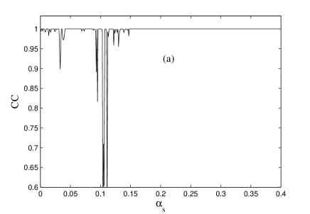
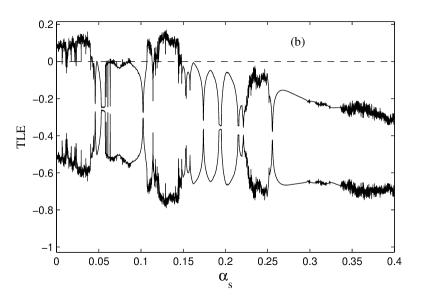
Figure 1: (a)Crosscorrelation (CC) between the two outer JJs for different values of coupling strength with all other values $\beta=0.3,i_{0}=1.2,\Omega=0.6,i_{dc}=0.3$ (b) Transverse Lyapunov exponents plotted for the same parameter values. $\tau$=0.1 in both cases.

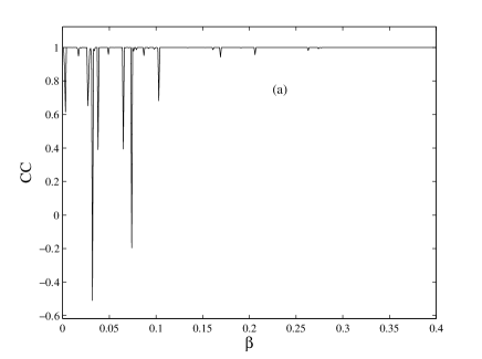
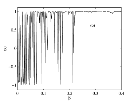
Figure 2: (a) CC between the two outer JJs for different values of damping parameter with $\alpha_{s}=0.37$ (b)CC between the outer and middle junction.

with $i=2,3.$ The value of correlation coefficient lies between $-1\leq CC\leq 1$ with large value of $\mid CC\mid$ meaning better synchrony. The cross correlation of the dynamics is shown in Fig.1(a) for the JJ system, from which we observe that for very low values of coupling constant there is loss of synchrony. In Fig.1(b) the transverse Lyapunov exponents are plotted. It can be seen that the sum of the TLE will always be negative as given by Eq.6.We observe that corresponding to the values where cross correlation is lost, there is a small positive value for one of the TLE. Fig.2 (a) shows the cross correlation between the outer junctions for various values of damping parameter. It can be observed from Fig.2 (b) that the middle junction remains uncorrelated with the outer ones for most of the values of damping parameter. Thus the middle junction mediates synchronization between the outer junction while remaining unsynchronized from both the outer junctions.

In the presence of a time-delay $\tau$, the dynamics of the system changes considerably. It is observed that for some values of time delay (for $\tau$ nearly equal to $0.35$ onwards) the system exhibits periodic synchronized motion. Fig. 3(a) is the bifurcation plot for various time-delays which shows periodic and chaotic behavior for different delay times. With Fig. 4(a), we show that the system remains synchronized for most of the values of time-delay. The TLEs plotted in Fig. 4(b)shows that one of the TLE has positive value for regions where CC is lost.

IV Effect of phase difference and frequency detuning

A phase difference between the applied fields was found to supress chaos effectively in an array of coupled Josephson junctions. In this section we study the effect of phase difference in bidirectionally coupled time-delay systems. From Eq. II, we can see that in the presence of an applied phase difference, the equation for the outer junctions is no longer identical. In terms of the difference variable $\psi_{1,3}^{-}=\psi_{1}-\psi_{3}$ we can write the equation for the outer junctions from Eq. II as

$$\dot{\psi}_{1,3}^{-}=-\beta\psi_{1,3}^{-}-2\cos(\frac{\phi_{1,3}^{+}}{2})\sin(\frac{\phi_{1,3}^{-}}{2})+i_{0}^{\prime}\sin(\Omega t+\theta/2)-\alpha_{s}\psi_{1,3}^{-}$$ (8)

where $\phi_{1,3}^{-}=\phi_{1}-\phi_{3}$, $\phi_{1,3}^{+}=\phi_{1}+\phi_{3}$ and $i_{0}^{\prime}=2i_{0}\sin(\theta/2)$ and it can be seen that for a finite value of phase difference the outer junctions cannot get synchronized.

The phase difference which usually desynchronizes the system may be used to suppress chaos in time-delayed systems. From Figs. 3 and 4, it can be seen that for a time delay of $\tau=0.25$ the system is chaotic and synchronized. Fig. 5 shows that an applied phase difference of $\theta=0.15\pi$ desynchronizes the system with $\tau=0$. But when a time-delay along with a phase difference is applied the system exhibits periodic motion. From the time series plotted in Fig. 6, it can be observed that the application of a phase difference $\theta=0.15\pi$ along with the time-delay, the system goes to a periodic state.

To complete the discussion, we consider the case of frequency detuning as it is difficult to apply a second frequency which is exactly same as the first. Small deviations in the applied frequencies are inevitable. So we consider the system with a small frequency detuning and the initial phase difference is taken to be zero. In order to investigate the difference in the dynamics brought about by frequency detuning, we first check the case where $\Delta\Omega=0$ in Eq.II, i.e, the case without any detuning. Fig. 7 shows the temporal dynamics of the system considered with no detuning. Fig. 7(a) shows the time series plot for $\psi_{1}$ with no detuning. Fig. 7(b) shows the time series plot for the difference between the variables of the outer and the middle junction while Fig. 7(c) is time series plot for the outer junctions. The outer junctions are perfectly synchronized while remaining uncorrelated with the inner junction.

When a frequency detuning is applied, it can be observed that the outer junctions show synchronization in regular intervals. Fig. 8(a) is the time series plot for the variable for the outer junction with $\Delta\Omega=0.004$ and it can be seen that a periodic modulation has appeared due to detuning. Here we observe that though the qualitative behavior is repeated, the trajectory of the system cannot be completely repeated due to the chaotic segments in the evolution process. This type of motion is referred to as breathers. Fig. 8(b) shows the time series plot for the difference between the variables of the outer and middle junctions and it can be seen that they remain uncorrelated. Fig. 8(c) shows the time series plot for the difference between the variables of the outer junctions. It can be seen that they get synchronized periodically with a period of $T=2\pi/\Delta\Omega$. The qualitative behavior of the system is not affected by time delays.

V Result and Discussion

In this work we deal with bidirectionally coupled time-delayed systems and study the effect of delay and phase difference between the applied fields on synchronization. The sum of the Lyapunov exponents transverse to the synchronization manifold is evaluated and it is found to be negative indicating the shrinking of phase space of the coupled system to a trajectory representing the synchronous state. However cross correlation coefficient reveals positive TLE for some values of coupling constant and damping parameter where synchrony is lost, though the sum would be still negative. Transverse Lyapunov exponents are evaluated numerically and are found to be in good agreement with the analytic results. By varying the time-delay, we have analyzed the behavior of the system and it is observed that for small values of time delays, periodic motion occur and as the delay time is increased chaotic motion reappears. However the system remained synchronized for most of the values of time-delay and hence may find applications in secure communication. The study on a configuration of three oscillators in a line is of importance because of the current recognition that it has resemblance with neuron models. Phase difference between the applied fields together with the time delays may be effectively used to suppress chaos. The practical situation where a small frequency detuning will be present between the applied fields is also studied. As the frequency detuning is like a time dependent phase difference, periodic and chaotic motions are repeated with a period of $T=2\pi/\Delta\Omega$. Time-delay does not change the effect of frequency detuning. Experimentally it is possible to apply a required delay in JJ kapl . Hence by suitably adjusting the time-delay, chaos may be controlled in JJ devices like voltage standards, detectors, SQUIDS etc where chaotic instabilities are least desired.

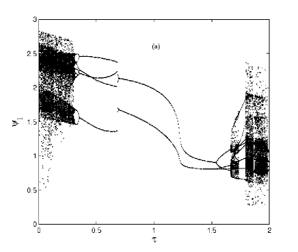
Figure 3: (a)Bifurcation diagram for $\psi_{1}$ against $\tau$ (b)Bifurcation diagram for $\psi_{2}$ against $\tau$. Parameter values are $\beta=0.3,i_{0}=1.2,\Omega=0.6,i_{dc}=0.3,\alpha_{s}=0.37$

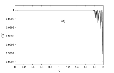
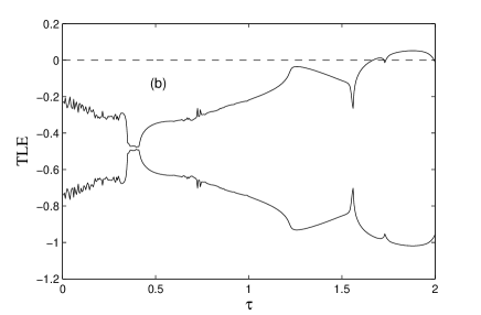
Figure 4: (a)Cross correlation for various values of $\tau$ with the other parameter values as $\beta=0.3,i_{0}=1.2,\Omega=0.6,i_{dc}=0.3,\alpha_{s}=0.37$ (b) TLEs plotted for different values of $\tau$

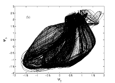
Figure 5: The outer and inner junctions are desynchronized on the application of a phase difference $\theta=0.15\pi$ with $\tau=0.$

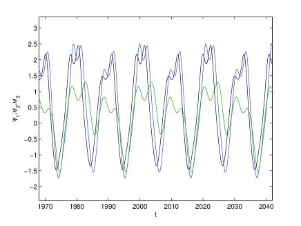
Figure 6: Periodic when a time delay $\tau=0.25$ along with a phase difference $\theta=0.15\pi$ applied.

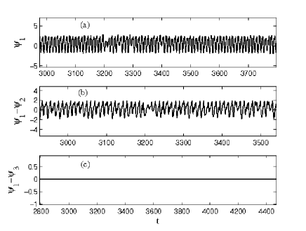
Figure 7: The temporal dynamics of the variable with no detuning for $\alpha=0.37$

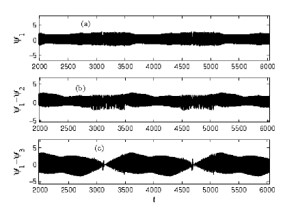
Figure 8: The temporal dynamics of the variable with $\Delta\Omega=0.004$ for $\alpha=0.37$

- (1) D. D’Humieres, M. R. Beasley, B. A. Huberman, and A. Libchaber, Phys. Rev. A26, 3483 (1982).
- (2) Y. Braiman and I. Goldhirsch, Phys. Rev. Lett. 66, 2545 (1991).
- (3) V. N. Belykh, N. F. Pedersen, and O. H. Soerensen, Phys. Rev. B 16, 4853 (1977).
- (4) V. N. Belykh, N. F. Pedersen, and O. H. Soerensen, Phys. Rev. B 16, 4860 (1977).
- (5) R. L. Kautz, Rep. Prog. Phys. 59, 935 (1996).
- (6) V. K. Kaplunenko, M. I. Khablpov and E. B. Goldobin, Supercond. Sci Technol.4, 674 (1991).
- (7) T. Yamada and H. Fujisaka, Prog. Theor. Phys. 69, 32 (1983).
- (8) T. Yamada and H. Fujisaka, Prog. Theor. Phys. 70, 1240 (1983).
- (9) L. M. Pecora and T. L. Carroll, Phys. Rev. Lett. 64, 821 (1990).
- (10) A. Pikovsky,M.Rosenblum and J.Kurths, Synchronization: A Universal concept in Nonlinear Science(Cambridge University press, Cambridge, 2001).
- (11) M. G. Rosenblum, A. S. Pikovsky, and J. Kurths, Phys. Rev. Lett. 78, 4193 (1997).
- (12) J.A.Blackburn, G.L.Baker and H.J.T.Smith, Phys. Rev. B 62, 5931 (2000).
- (13) Ahmet Uçar, Karl E. Lonngren and Er-Wei Bai, Chaos, Solitons and Fractals 31, 105 (2007).
- (14) Chitra R Nayak and V.C. Kuriakose, Phys.Lett.A 365, 284 (2007).
- (15) Feng Cun-Fang, Zhang Yan and Wang Ying-Lai, Chin.Phys.Lett. 23, 1418 (2006).
- (16) Feng Cun-Fang, Zhang Yan and Wang Ying-Lai, Chin.Phys.Lett.24, 50 (2007).
- (17) D. V. Senthilkumar, M. Lakshmanan, and J. Kurths, Phys. Rev. E 74, 035205 (2006).
- (18) N.Krasovskii, Stability of motion, Stanford press, Stanford, 1963.
- (19) K.Pyragas, Phys. Rev. E 58, 3067 (1998).
- (20) D. V. Senthilkumar and M. Lakshmanan, Chaos 17, 013112 (2007).
- (21) V. M. Eguìluz, D. R. Chialvo, G. A. Cecchi, M. Baliki, and A. V. Apkarian, Phys. Rev. Lett. 94, 018102 (2005).
- (22) I. Fischer, R. Vicente, J. M. Buldú, M. Peil, C. R. Mirasso, M. C. Torrent and Jordi Garc a-Ojalvo, Phys. Rev. Lett. 97, 123902 (2006).
- (23) Alexandra S. Landsman and Ira B. Schwartz, Phys. Rev. E 75 , 026201 (2007).
- (24) Ira B. Schwartz and Leah B Shaw, Phys. Rev. E 75 , 046207 (2007).
- (25) A. Barone and G. Paterno, Physics and Applications of Josephson effect, (New York:Wiley & sons,1982).
- (26) G. V. Osipov, A. S. Pikovsky, and J. Kurths, Phys. Rev. Lett. 88, 054102 (2002).
- (27) Chitra R. N. and V.C. Kuriakose, Chaos 18, 013125 (2008).