Optical and dc transport properties of a strongly correlated charge density wave system: exact solution in the ordered phase of the spinless Falicov-Kimball model with dynamical mean-field theory

Abstract

We derive the dynamical mean-field theory equations for transport in an ordered charge-density-wave phase on a bipartite lattice. The formalism is applied to the spinless Falicov-Kimball model on a hypercubic lattice at half filling. We determine the many-body density of states, the dc charge and heat conductivities, and the optical conductivity. Vertex corrections continue to vanish within the ordered phase, but the density of states and the transport coefficients show anomalous behavior due to the rapid development of thermally activated subgap states. We also examine the optical sum rule and sum rules for the first three moments of the Green’s functions within the ordered phase and see that the total optical spectral weight in the ordered phase either decreases or increases depending on the strength of the interactions.

I Introduction

Dynamical mean-field theory was introduced almost two decades ago by Brandt and Mielschbrandt_mielsch1 , who solved for the transition temperature into a charge-density-wave (CDW) phase of the spinless Falicov-Kimball model at half filling. This work appeared shortly after the idea of examining strongly correlated electrons in the limit of infinite dimensions was introducedmetzner_vollhardt . Since then, the field of DMFT has emerged as one of the most powerful nonperturbative techniques for solving the many-body problem. While results for many properties exist in the homogeneous (unordered) phasekotliar_review , there has been little work in examining the properties of the ordered phase. Brandt and Mielsch worked out the formalism for calculating ordered-phase Green’s functionsbrandt_mielsch2 , the order parameter was shown to display anomalous behavior at weak couplingvandongen ; chen_freericks , and higher-period ordered phases have been examined on the Bethe latticefreericks_swiss . But, surprisingly, there has been no work on the transport properties in the ordered phase. Indeed, it is interesting to compare how transport varies in the homogeneous phase versus the ordered phase. At weak coupling, we anticipate the gap formation of the CDW to greatly suppress the dc transport, while at strong coupling it may be a much milder correction to the Mott-insulating behavior. What is more interesting is to examine the temperature dependence. For example, in systems that are metallic at high temperature, the many-body DOS in the CDW phase develops strong temperature dependence (with increasing $T$) as the CDW gap region fills in due to thermal excitations, until gap closure is complete at the transition temperature. But unlike the well-known superconducting case, where subgap states tend not to form and the gap is simply reduced in size as $T$ increases, here we have a rapid development of subgap states, even though the CDW order parameter remains nonzero. These subgap states should produce anomalous behavior in the low-$T$ transport, and indeed we find this is so but the quantitative behavior is not that different from exponential activation of the transport. We anticipate our results should be relevant to different experimental systems that display charge-density-wave order, especially in compounds which are three-dimensional likecdw_exp BaBiO₃ and Ba_1-xK_xBiO₃.

This contribution is organized as follows: In Section II, we present the formalism for DMFT in the ordered phase including the techniques needed to determine the optical conductivity and the dc transport. We also determine moment sum rules for the Green’s functions in the ordered phase. In Section III, we apply the formalism to numerical solutions of the Falicov-Kimball model at half filling and show how the transport behaves in the ordered phases. Conclusions and a discussion follow in Section IV.

II Formalism for the ordered phase

The Falicov-Kimball modelfalicov_kimball was introduced in 1969 as a model for metal-insulator transitions in rare-earth compounds and transition-metal oxides. The spinless version is arguably the simplest many-body problem that nevertheless possesses rich physics including the Mott transition, order-disorder phase transitions, and phase separation (for a review see Ref. freericks_review, ). It involves two kinds of electrons: mobile conduction electrons whose creation and destruction operators are $\hat{d}_{i}^{\dagger}$ and $\hat{d}_{i}$ at site $i$; and localized electrons whose creation and destruction operators are $\hat{f}_{i}^{\dagger}$ and $\hat{f}_{i}$ at site $i$. The Falicov-Kimball Hamiltonian can be represented in terms of a local operator and a hopping operator as follows

$$\mathcal{\hat{H}}=\sum_{i}\mathcal{\hat{H}}_{i}-\sum_{ij}t_{ij}\hat{d}_{i}^{{\dagger}}\hat{d}_{j},$$ (1)

where $t_{ij}$ is the hopping matrix and

$$\mathcal{\hat{H}}_{i}=U\hat{n}_{id}\hat{n}_{if}-\mu_{d}\hat{n}_{id}-\mu_{f}\hat{n}_{if},$$ (2)

is the local Hamiltonian with the number operators given by $\hat{n}_{id}=\hat{d}_{i}^{\dagger}\hat{d}_{i}$ and $\hat{n}_{if}=\hat{f}_{i}^{\dagger}\hat{f}_{i}$.

If the lattice can be divided into two sublattices, and the hopping is nonzero only between the two sublattices (i. e., there is no hopping within either sublattice), then the lattice is called a bipartite lattice, and it has nesting at half filling in the noninteracting system, which implies the fermi surface in the Brillouin zone has flat regions that are connected by the zone-diagonal wavevector $Q=(\pi,\pi,\ldots)$. Nesting promotes the formation of a CDW with the average filling of the electrons being uniform on each sublattice, but changing from one sublattice to another. This is often called the checkerboard or chessboard CDW, and is the ordered phase that we will examine in detail in this work.

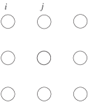
  $\to$  

Figure 1: Schematic illustration of the transition from a homogeneous phase to the bipartite CDW phase. The hopping is between nearest neighbors, which corresponds to the neighboring points in the horizontal and vertical directions.

In order to develop the formalism to determine the Green’s functions and transport in the ordered CDW phase, we need to introduce some notation that will help clarify how the ordered phase is determined. It is convenient to supplement the lattice site index, which we had been calling $i$, by a double index $(i,a)$, where $i$ runs over all of the lattice sites of one of the sublattices, and the label $a=A$ or $B$ denotes the sublattice (see Fig. 1; we are assuming for simplicity that the two sublattices have an equal number of lattice sites as they do on the infinite-dimensional hypercubic lattice or on the infinite-coordination-number Bethe lattice). We rewrite the Hamiltonian from Eq. (1) as

$$\mathcal{\hat{H}}=\sum_{ia}\mathcal{\hat{H}}_{i}^{a}-\sum_{ijab}t_{ij}^{ab}\hat{d}_{ia}^{{\dagger}}\hat{d}_{jb},$$ (3)

with the local Hamiltonian satisfying

$$\mathcal{\hat{H}}_{i}^{a}=U\hat{n}_{id}^{a}\hat{n}_{if}^{a}-\mu_{d}^{a}\hat{n}_{id}^{a}-\mu_{f}^{a}\hat{n}_{if}^{a};$$ (4)

in this notation, the bipartite lattice condition is simply that $t_{ij}^{AA}=t_{ij}^{BB}=0$. We have introduced different chemical potentials for the two different sublattices at the moment. This is convenient for computations, because it allows us to work with a fixed order parameter, rather than iterating the DMFT equations to determine the order parameter (which is subject to critical slowing down near $T_{c}$). Of course, the equilibrium solution occurs when the chemical potential is uniform throughout the system ($\mu^{A}_{d}=\mu^{B}_{d}$ and $\mu^{A}_{f}=\mu^{B}_{f}$).

Our starting point is to find the set of equations satisfied by the lattice Green’s function. The Green’s function is defined to be

$$G_{ij}^{ab}(\tau)=-\operatorname{Tr}\left[\mathcal{T}_{\tau}e^{-\beta\mathcal{\hat{H}}}\hat{d}_{ia}(\tau)\hat{d}^{\dagger}_{jb}(0)\right]/\mathcal{Z},$$ (5)

where $\tau$ is the imaginary time, the time dependence of the destruction operator is written in the Heisenberg representation {$d_{ia}(\tau)=\exp[\tau\mathcal{\hat{H}}]d_{ia}\exp[-\tau\mathcal{\hat{H}}]$}, and $\mathcal{Z}$ is the partition function $\mathcal{Z}=\operatorname{Tr}\exp[-\beta\mathcal{\hat{H}}]$, with $\beta=1/T$ the inverse temperature. The symbol $\mathcal{T}_{\tau}$ is the time-ordering operator, which orders the times so that earlier times appear to the right.

One way to calculate the Green’s function is to use an equation of motion techniquezlatic_review , where the derivative with respect to imaginary time is taken and a differential equation is found for the Green’s function. In DMFT, this procedure is carried out for the impurity problem in a time-dependent field, and the field is adjusted so that the impurity Green’s function is equal to the local lattice Green’s function. In addition, we need to define the self-energy via Dyson’s equation in order to complete the iterative DMFT loop needed to solve the full problem. Finally, an analytic continuation from the imaginary axis to the real axis is performed to calculate dynamical properties. These techniques are all well known and have been established in the literaturebrandt_mielsch1 ; brandt_mielsch2 ; zlatic_review ; freericks_review , so we provide just a schematic approach to the derivation, highlighting some key formulas along the way.

The Dyson equation, which can be thought of as defining the self-energy is

$$\sum_{lc}[(\omega+\mu^{a}_{d})\delta_{ac}\delta_{il}-\Sigma_{il}^{ac}(\omega)+t^{ac}_{il}]G_{lj}^{cb}(\omega)=\delta_{ij}\delta_{ab},$$ (6)

with $\omega$ the real frequency. In the case of nearest-neighbor hopping on an infinite-dimensional hypercubic lattice, we have that the band structure satisfies $\epsilon_{\bm{k}}=-\sum_{j}\exp[i{\bf k}\cdot({\bf R}_{iA}-{\bf R}_{jB})]t_{ij}^{AB}=-\lim_{D\rightarrow\infty}t^{*}\sum\limits_{\alpha=1}^{D}\cos{k_{\alpha}}/\sqrt{D}$, where we scaledmetzner_vollhardt the nearest neighbor hopping matrix element by $t=t^{*}/2\sqrt{D}$ (we will use $t^{*}=1$ as our energy unit). In addition, the self-energy is localmetzner

$$\Sigma_{ij}^{ab}(\omega)=\Sigma_{i}^{a}(\omega)\delta_{ij}\delta_{ab},$$ (7)

which further simplifies the Dyson equation. It is simpler to transform from real space to momentum space to solve the Dyson equation. But we do not assume that the Green’s function is completely translation invariant, instead, we assume only that there is translation invariance within each of the sublattices. Then the momentum representation of the Dyson equation in Eq. (6) with the local self-energy in Eq. (7) becomes

$${G}_{\bm{k}}(\omega)=\left[{z}(\omega)-{t}_{\bm{k}}\right]^{-1},$$ (8)

where $z(\omega)$ and the hopping term are represented by $2\times 2$ matrices

$${z}(\omega) =\left(\begin{array}[]{cccc}\omega+\mu^{A}_{d}-\Sigma^{A}(\omega)&0\\ 0&\omega+\mu^{B}_{d}-\Sigma^{B}(\omega)\\ \end{array}\right),$$ (11)

$${t}_{\bm{k}} =\left(\begin{array}[]{cccc}0&\epsilon_{\bm{k}}\\ \epsilon_{\bm{k}}&0\\ \end{array}\right).$$ (14)

Substituting Eq. (14) into Eq. (8) and taking the matrix inverse yields the following formulas for the momentum-dependent Green’s functions on the lattice

$$G_{\bm{k}}^{AA}(\omega) =\dfrac{\omega+\mu^{B}_{d}-\Sigma^{B}(\omega)}{\bar{Z}^{2}(\omega)-\epsilon^{2}_{\bm{k}}},$$ (15)

$$G_{\bm{k}}^{BB}(\omega) =\dfrac{\omega+\mu^{A}_{d}-\Sigma^{A}(\omega)}{\bar{Z}^{2}(\omega)-\epsilon^{2}_{\bm{k}}},$$ (16)

$$G_{\bm{k}}^{AB}(\omega) =G_{k}^{BA}(\omega)=\dfrac{\epsilon_{\bm{k}}}{\bar{Z}^{2}(\omega)-\epsilon^{2}_{\bm{k}}}$$ (17)

with $\bar{Z}$ defined by

$$\bar{Z}(\omega)=\sqrt{[\omega+\mu^{A}_{d}-\Sigma^{A}(\omega)][\omega+\mu^{B}_{d}-\Sigma^{B}(\omega)]},$$ (18)

which agree with those of Brandt and Mielschbrandt_mielsch2 even though our notation is somewhat different from theirs. The local Green’s functions on each sublattice then satisfy

$$G^{aa}(\omega)=\dfrac{\omega+\mu^{b}_{d}-\Sigma^{b}(\omega)}{\bar{Z}(\omega)}F_{z}(\omega),$$ (19)

where the $a$ sublattice is different from the $b$ sublattice and $F_{z}(\omega)$ is the Hilbert transform

$$F_{z}(\omega)=\int d\epsilon\rho(\epsilon)\frac{1}{\bar{Z}(\omega)-\epsilon}.$$ (20)

The function $\rho(\epsilon)$ is the noninteracting density of states, which is $\rho(\epsilon)=\exp(-\epsilon^{2}/t^{*2})/t^{*}\sqrt{\pi}$ for the infinite-dimensional hypercubic lattice (as discussed above, we take $t^{*}=1$).

In the DMFT solution, we need to map the lattice problem onto a local (impurity) problem in a time-dependent field that is adjusted to make the impurity Green’s function equal to the local Green’s function of the lattice. Here, we have two different local Green’s functions, one on the A sublattice and one on the B sublattice; hence we will need two time dependent fields and two impurity problems to solve in order to complete the DMFT mapping. We call the dynamical mean fields $\lambda^{a}(\omega)$ for each sublattice. Then the solution of the impurity problem is straightforward and is summarized by the following set of equations

$$G^{a}_{0}(\omega) =\left[G^{aa}(\omega)^{-1}+\Sigma^{a}(\omega)\right]^{-1}$$ (21)

$$=\frac{1}{\omega+\mu^{a}_{d}-\lambda^{a}(\omega)},$$ (22)

$$G^{aa}(\omega) =\frac{(1-n_{f}^{a})}{\omega+\mu^{a}_{d}-\lambda^{a}(\omega)}$$

$$+\frac{n_{f}^{a}}{\omega+\mu^{a}_{d}-U-\lambda^{a}(\omega)},$$ (23)

$$\Sigma^{a}(\omega) =\omega+\mu_{d}^{a}-\lambda^{a}(\omega)-G^{aa}(\omega)^{-1},$$ (24)

where we must solve these equations for each of the sublattices $a=A$ and $a=B$.

The DMFT algorithm for a fixed value of the order parameter starts by choosing $n_{f}^{A}$ and $n_{f}^{B}$ such that $n_{f}^{A}+n_{f}^{B}$ is fixed to the total $f$-electron filling (the order parameter is $\Delta n_{f}=n_{f}^{A}-n_{f}^{B}$), and choosing $\mu_{d}^{A}=\mu_{d}^{B}$. With those fixed quantities, we propose a guess for the self-energy on each sublattice, and then compute the local Green’s function on the real axis from Eqs. (18) and (19). Then we extract the dynamical mean field on each sublattice from Eqs. (21) and (22), then find the local Green’s function for the impurity from Eq. (23) and the new self-energy from Eq. (24). This loop is repeated until the Green’s functions converge. Then one can calculate the filling of the $d$-electrons and adjust them until they match the target filling. But this procedure is not yet complete, because we need to determine the correct equilibrium order parameter $n_{f}^{A}-n_{f}^{B}$ at the given temperature. To find this, it is actually more convenient to perform the calculations precisely as described above, but on the imaginary frequency axis, where $\omega$ is replaced by $i\omega_{n}=i\pi T(2n+1)$ the fermionic Matsubara frequencies. Then we calculate the chemical potential for the $f$-electrons on each sublattice via

$$\mu^{a}_{f}=-\frac{U}{2}-T\ln\frac{1-n_{f}^{a}}{n_{f}^{a}}-T\sum_{n}\ln[1-UG_{0}^{a}(i\omega_{n})],$$ (25)

and adjust the order parameter until the two chemical potentials are equal, which is required for the equilibrium solution. Then, when we calculate the Green’s functions on the real axis, the chemical potentials and fillings are all already known, so they do not need to be adjusted during the calculation.

This algorithm is much more efficient than an algorithm that starts with a fixed chemical potential for the $f$-electrons and iterates to determine $n_{f}^{a}$ on the imaginary frequency axis. This is because the latter suffers from critical slowing down, and becomes quite inefficient near the critical temperature, whereas the calculations with the fixed order parameter converge quite rapidly regardless of how close one is to the critical point.

When the DOS is calculated for each sublattice in the ordered phase, one finds interesting temperature dependence of the subgap states as a function of $T$. It is illustrative to discuss these evolutions in terms of the moments of the local interacting DOS. It is well known, that in the homogeneous phase, the integral of $A(\omega)=-\operatorname{Im}G(\omega)/\pi$ is equal to 1. But there are also exact results known for higher moments as wellwhite_moment ; freericks_moment . In particular, because the moments are derived from operator identities, they continue to hold whether in the ordered phase or not. So we learn the following identities immediately:

$$\int d\omega A^{a}(\omega) =1;$$ (26)

$$\int d\omega\omega A^{a}(\omega) =-\mu_{d}^{a}+Un_{f}^{a};$$ (27)

$$\int d\omega\omega^{2}A^{a}(\omega) =\frac{1}{2}+\mu_{d}^{a2}-2U\mu_{d}^{a}n_{f}^{a}+U^{2}n_{f}^{a}.$$ (28)

We have checked these moments versus our numerical calculations of the Green’s functions on the real axis and they all agree to high accuracy for all temperatures that we consider. Note that at half filling, we have $\mu_{d}^{a}=U/2$, so the first moment vanishes in the homogeneous phase. As the system orders, the first moment on one sublattice becomes negative, and the first moment on the other sublattice becomes positive, which indicates that the quantum states are shifting in response to the ordering. In particular, this redistribution of states causes the average kinetic energy to evolve more strongly with temperature in the ordered phase, but its evolution is anomalous, and cannot be predicted by any simple reasoning about how the states evolve (see below). The evolution of the average kinetic energy plays an important role in the total spectral weight for the optical conductivity.

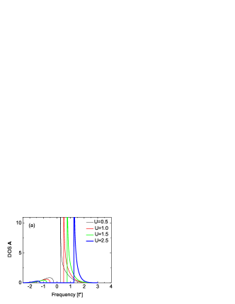
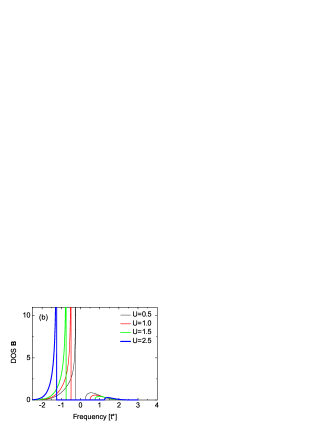
Figure 2: (Color online) DOS at $T=0$ for the CDW-ordered phase on a hypercubic lattice. Panel (a) is for the $A$ sublattice and panel (b) is for the $B$ sublattice. Four cases are plotted: $U=0.5$ which is a strongly correlated metal; $U=1$, where a dip develops in the normal-state DOS at the chemical potential; $U=1.5$, which is a near-critical Mott insulator; and $U=2.5$, which is a moderate-size-gap Mott insulator. The $T=0$ gap in the DOS is always equal to $U$ in the ordered CDW phase.

At $T=0$, the order parameter goes to 1, so there is one sublattice (let us say the $A$ sublattice) which has all the $f$-electrons. Hence $n_{f}^{A}=1$ and $n_{f}^{B}=0$. In this case, the analysis for the Green’s function simplifies. In particular, only one term in Eq. (23) survives on each sublattice and we immediately find $\Sigma^{A}=U$ and $\Sigma^{B}=0$. Plugging these results into the remaining formulas for the DMFT algorithm then yields an analytic formula for the ordered phase DOS

$$A_{A,B}(\omega) =-\frac{1}{\pi}\operatorname{Im}G^{AA,BB}(\omega)$$

$$=\operatorname{Re}\left[\sqrt{\frac{\omega\pm\frac{U}{2}}{\omega\mp\frac{U}{2}}}\right]\rho\left(\sqrt{\omega^{2}-\frac{U^{2}}{4}}\right),$$ (29)

where the top sign is for the $A$ sublattice (with a divergence of the DOS at $\omega=U/2$) and the bottom sign is for the $B$ sublattice (with a divergence at $\omega=-U/2$); the formula is restricted to half filling where $\mu_{d}^{A}=\mu_{d}^{B}=U/2$. Note that the two DOS on each sublattice are mirror images of each other and that each sublattice has weight for positive and negative frequency, but the band that does not have the singularity (lower band for sublattice $A$ and upper band for sublattice $B$) has shrinking spectral weight as $U$ becomes large, because the mobile electrons avoid the sites with the localized electrons for large $U$. Note further, that unlike the Mott insulator, where the DOS vanishes only at the chemical potential on a hypercubic lattice, a real gap develops here of magnitude $U$ at $T=0$. In Fig. 2, we show the DOS at zero temperature for four values of $U$. Panel (a) plots the DOS on the $A$ sublattice and panel (b) plots the DOS on the $B$ sublattice. One can see that the shape of the DOS is qualitatively similar for all cases, but the size of the gap grows with $U$.

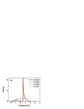
Figure 3: (Color online) DOS on the A sublattice for various $T$ values in the CDW-ordered phase on a hypercubic lattice with (a) $U=0.5$ and (b) $U=1$. The DOS on the B sublattice is a mirror reflection of these results about the plane $\omega=0$.

What is more interesting is to examine the temperature evolution of the DOS in these different cases. Indeed, the system develops substantial subgap DOS that is thermally excited within the ordered phase (the order parameter is determined by the difference in localized electron filling on the two sublattices). In Fig. 3 (a), we plot the DOS for the strongly correlated metal at $U=0.5$. The fill in of the subgap states is quite rapid with $T$ as we increase up to $T_{c}=0.0336$. Similar behavior is also observed for $U=1$ with $T_{c}=0.0615$ which has a dip in the DOS in the normal state [Fig. 3 (b)].

The Mott insulating phases also illustrate interesting behavior. In particular, the subgap states develop primarily within the upper and lower Hubbard bands (although on the hypercubic lattice, the Mott insulator has only a pseudogap with the DOS strictly vanishing only at $\omega=0$). We illustrate this behavior in Figs. 4 (a) and (b). The transition temperatures are $T_{c}=0.0747$ for $U=1.5$ and $T_{c}=0.0724$ for $U=2.5$. Note how the subgap DOS develop closer to the Mott band edge than they do to the CDW band edge, which implies they should have an effect on the transport at low $T$.

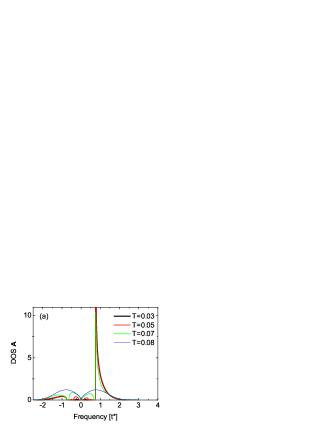
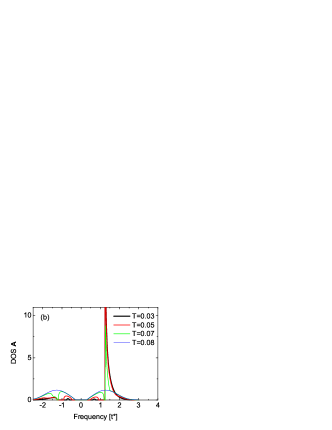
Figure 4: (Color online) DOS on the A sublattice for various $T$ values in the CDW-ordered phase on a hypercubic lattice with (a) $U=1.5$ and (b) $U=2.5$.

In all cases, the DOS satisfy the three sum rules for the first three moments to essentially machine accuracy—our actual accuracy is determined by the step size we use for the real frequency axis in calculating the DOS and then integrating it over all frequency to obtain the numerical moments.

Now we develop the formalism for transport in the CDW phase. The linear response optical conductivity is determined (via the Kubo-Greenwood formulakubo ; greenwood ) by the imaginary part of the analytic continuation of the current-current correlation function to the real axis,

$$\sigma(\omega)=\dfrac{1}{\omega}\operatorname{Im}{\Pi_{jj}(\omega)},$$ (30)

with the number current operators defined by

$${\bm{\hat{j}}} =i\sum_{ijab}t_{ij}^{ab}(\bm{R}_{ia}-\bm{R}_{jb})\hat{d}_{ia}^{{\dagger}}\hat{d}_{jb},$$ (31)

$$j_{\alpha} =\sum\limits_{ab\bm{k}}\dfrac{\partial\epsilon_{\bm{k}}^{ab}}{\partial k_{\alpha}}d_{a}^{{\dagger}}(\bm{k})d_{b}(\bm{k}).$$ (32)

The procedure to determine the current-current correlation function is a standard one so we only sketch the derivation briefly. We start from the imaginary time formula for the current-current correlation function

$$\Pi_{jj}(\tau-\tau^{\prime})=\left\langle T_{\tau}j(\tau)j(\tau^{\prime})\right\rangle,$$ (33)

where the angle brackets denote a trace over all states weighted by the statistical operator (density matrix) at the given temperature and the current operators are represented in the Heisenberg representation with respect to the equilibrium Hamiltonian (because this is a linear-response calculation). We then perform a Fourier transformation to go from imaginary time to Matsubara frequencies, and then perform an analytic continuation from the imaginary frequency axis to the real frequency axis.

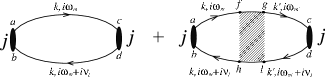
Figure 5: Bethe-Salpeter equation for the generalized polarization.

The Fourier transform of the current-current correlation function defined in Eq. (33) can be represented as a summation over Matsubara frequencies

$$\Pi_{jj}(i\nu_{l})=T\sum\limits_{m}\Pi_{m,m+l}$$ (34)

where we introduced the shorthand notation $\Pi_{m,m+l}=\Pi(i\omega_{m},i\omega_{m}+i\nu_{l})$ for the dependence on the fermionic $i\omega_{m}=i\pi T(2m+1)$ and bosonic $i\nu_{l}=i2\pi Tl$ Matsubara frequencies ($m$ and $l$ are integers). In the CDW phase, the graphic depiction of the Bethe-Salpeter equation for the generalized polarization $\Pi_{m,m+\nu}$ is plotted in Fig. 5 where the solid oval depicts the current operator using the same sublattice indices as we have used before (the current operator connects the two sublattices), the solid lines are Green’s functions, and the cross hatched object is the total (reducible) charge vertex. The current operator vertex contains the factor $\partial\epsilon_{\bm{k}}/\partial k_{\alpha}$ which is an odd function of the wavevector. Since the band structure $\epsilon_{\bm{k}}$ and the Green’s functions are even functions of the wavevector, any summation over momentum that contains one current vertex and any number of Green’s functions will vanish. Now, in infinite dimensions, the irreducible charge vertex (which enters the Bethe-Salpeter equation for the total charge vertex) is local and hence momentum independent, so the second term in Fig. 5 vanishes, just like it did in the homogeneous phasekhurana . We thereby conclude that the optical conductivity is constructed only by the bare bubble in Fig. 5.

$\Large{\Pi_{m,m+l}=\sum\limits_{abcd}}$
=
+

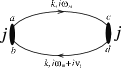
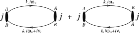
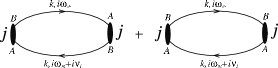
Figure 6: Individual terms for the bare polarization in the ordered phase.

Then, the full expression for the generalized polarization $\Pi_{m,m+l}$ is depicted in Fig. 6 and simplifies to

$$\Pi_{m,m+l} =\frac{1}{N}\sum_{\bm{k}}j_{\bm{k}}^{2}(G_{\bm{k}m}^{AA}G_{\bm{k}m+l}^{BB}+G_{\bm{k}m}^{AB}G_{\bm{k}m+l}^{AB}$$

$$+G_{\bm{k}m}^{BA}G_{\bm{k}m+l}^{BA}+G_{\bm{k}m}^{BB}G_{\bm{k}m+l}^{AA}),$$ (35)

where $j_{\bm{k}}=-\lim_{D\rightarrow\infty}(t^{*}/\sqrt{D})\sum_{r=1}^{D}\sin k_{r}$ and solid lines denote the momentum-dependent lattice Green’s functions $G_{\bm{k}m}^{ab}$ [see Eqs. (15–17)]. After substituting in the expressions for the Green’s functions, the individual contributions to $\Pi_{m,m+l}$ become

$$\dfrac{1}{N}\sum\limits_{\bm{k}}j_{\bm{k}}^{2}G_{\bm{k}m}^{AA}G_{\bm{k}m+l}^{BB}=\dfrac{1}{2}(i\omega_{m}+\mu_{d}^{B}-\Sigma_{m}^{B})$$

$$\times (i\omega_{m}+i\nu_{l}+\mu_{d}^{A}-\Sigma_{m+l}^{A})\dfrac{\dfrac{F_{z}(i\omega_{m+l})}{\bar{Z}(i\omega_{m+l})}-\dfrac{F_{z}(i\omega_{m})}{\bar{Z}(i\omega_{m})}}{\bar{Z}^{2}(i\omega_{m})-\bar{Z}^{2}(i\omega_{m+l})},$$

$$\dfrac{1}{N}\sum\limits_{\bm{k}}j_{\bm{k}}^{2}G_{\bm{k}m}^{BB}G_{\bm{k}m+l}^{AA}=\dfrac{1}{2}(i\omega_{m}+\mu_{d}^{A}-\Sigma_{m}^{A})$$

$$\times (i\omega_{m}+i\nu_{l}+\mu_{d}^{B}-\Sigma_{m+l}^{B})\dfrac{\dfrac{F_{z}(i\omega_{m+l})}{\bar{Z}(i\omega_{m+l})}-\dfrac{F_{z}(i\omega_{m})}{\bar{Z}(i\omega_{m})}}{\bar{Z}^{2}(i\omega_{m})-\bar{Z}^{2}(i\omega_{m+l})},$$

$$\dfrac{1}{N}\sum\limits_{\bm{k}}j_{\bm{k}}^{2}G_{\bm{k}m}^{AB}G_{\bm{k}m+l}^{AB}=\dfrac{1}{N}\sum\limits_{\bm{k}}j_{\bm{k}}^{2}G_{\bm{k}m}^{BA}G_{\bm{k}m+l}^{BA}$$

$${}= \dfrac{1}{2}\dfrac{\bar{Z}(i\omega_{m+l})F_{z}(i\omega_{m+l})-\bar{Z}(i\omega_{m})F_{z}(i\omega_{m})}{\bar{Z}^{2}(i\omega_{m})-\bar{Z}^{2}(i\omega_{m+l})}.$$ (36)

Hence, the full expression for $\Pi_{m,m+l}$ is

$$\Pi_{m,m+l} =\dfrac{1}{2}\Biggl{\{}\frac{\dfrac{F_{z}(i\omega_{m+l})}{\bar{Z}(i\omega_{m+l})}-\dfrac{F_{z}(i\omega_{m})}{\bar{Z}(i\omega_{m})}}{\bar{Z}^{2}(i\omega_{m})-\bar{Z}^{2}(i\omega_{m+l})}$$

$$\times\biggl{[}(i\omega_{m}+\mu_{d}^{B}-\Sigma_{m}^{B})(i\omega_{m}+i\nu_{l}+\mu_{d}^{A}-\Sigma_{m+l}^{A})$$

$$+(i\omega_{m}+\mu_{d}^{A}-\Sigma_{m}^{A})(i\omega_{m}+i\nu_{l}+\mu_{d}^{B}-\Sigma_{m+l}^{B})\biggr{]}$$

$$+2\dfrac{\bar{Z}(i\omega_{m+l})F_{z}(i\omega_{m+l})-\bar{Z}(i\omega_{m})F_{z}(i\omega_{m})}{\bar{Z}^{2}(i\omega_{m})-\bar{Z}^{2}(i\omega_{m+l})}\Biggr{\}}.$$ (37)

Then, the expression for the current-current Green’s function is obtained by substituting Eq. (II) into Eq. (34) and analytically continuing the summation over Matsubara frequencies into contour integrations

$$\Pi_{jj}(i\nu_{l}) =\frac{1}{2\pi i}\int\limits_{-\infty}^{+\infty}d\tilde{\omega}f(\tilde{\omega})$$

$$\times\Big{[}\Pi(\tilde{\omega}-i0^{+},\tilde{\omega}+i\nu_{l})-\Pi(\tilde{\omega}+i0^{+},\tilde{\omega}+i\nu_{l})$$

$$+\Pi(\tilde{\omega}-i\nu_{l},\tilde{\omega}-i0^{+})-\Pi(\tilde{\omega}-i\nu_{l},\tilde{\omega}+i0^{+})\Big{]}.$$ (38)

Here we have $f(\tilde{\omega})=1/[1+\exp(\beta\tilde{\omega})]$ is the fermi distribution function. The final step is to analytically continue from the bosonic Matsubara frequencies to the real axis ($i\nu\to\omega\pm i0^{+}$). This produces our final result

$$\Pi_{jj}(\omega) =\dfrac{2}{(2\pi i)^{2}}\int\limits_{-\infty}^{+\infty}d\tilde{\omega}\left[f(\tilde{\omega})-f(\tilde{\omega}+\omega)\right]$$

$$\times\operatorname{Re}\{\Pi(\tilde{\omega}-i0^{+},\tilde{\omega}+\omega+i0^{+})$$

$$-\Pi(\tilde{\omega}-i0^{+},\tilde{\omega}+\omega-i0^{+})\}.$$ (39)

To make Eq. (39) concrete, we substitute in the analytic continuation of Eq. (II) to find the final expression for the optical conductivity (we set $e^{2}=1$):

$$\sigma(\omega) =\dfrac{1}{4\pi^{2}}\int\limits_{-\infty}^{+\infty}d\tilde{\omega}\dfrac{\left[f(\tilde{\omega})-f(\tilde{\omega}+\omega)\right]}{\omega}$$

$$\times\operatorname{Re}\Biggl{\{}\dfrac{\dfrac{F^{*}_{z}(\tilde{\omega}+\omega)}{\bar{Z}^{*}(\tilde{\omega}+\omega)}-\dfrac{F_{z}(\tilde{\omega})}{\bar{Z}(\tilde{\omega})}}{\bar{Z}^{2}(\tilde{\omega})-[\bar{Z}^{*}(\tilde{\omega}+\omega)]^{2}}$$

$$\times\biggl{(}[\tilde{\omega}+\mu_{d}^{B}-\Sigma^{B}(\tilde{\omega})][\tilde{\omega}+\omega+\mu_{d}^{A}-\Sigma^{A*}(\tilde{\omega}+\omega)]$$

$$+[\tilde{\omega}+\mu_{d}^{A}-\Sigma^{A}(\tilde{\omega})][\tilde{\omega}+\omega+\mu_{d}^{B}-\Sigma^{B*}(\tilde{\omega}+\omega)]\biggl{)}$$

$$+2\dfrac{\bar{Z}^{*}(\tilde{\omega}+\omega)F_{z}^{*}(\tilde{\omega}+\omega)-\bar{Z}(\tilde{\omega})F_{z}(\tilde{\omega})}{\bar{Z}^{2}(\tilde{\omega})-[\bar{Z}^{*}(\tilde{\omega}+\omega)]^{2}}$$

$$-\dfrac{\dfrac{F_{z}(\tilde{\omega}+\omega)}{\bar{Z}(\tilde{\omega}+\omega)}-\dfrac{F_{z}(\tilde{\omega})}{\bar{Z}(\tilde{\omega})}}{\bar{Z}^{2}(\tilde{\omega})-\bar{Z}^{2}(\tilde{\omega}+\omega)}$$

$$\times\biggl{(}[\tilde{\omega}+\mu_{d}^{B}-\Sigma^{B}(\tilde{\omega})][\tilde{\omega}+\omega+\mu_{d}^{A}-\Sigma^{A}(\tilde{\omega}+\omega)]$$

$$+[\tilde{\omega}+\mu_{d}^{A}-\Sigma^{A}(\tilde{\omega})][\tilde{\omega}+\omega+\mu_{d}^{B}-\Sigma^{B}(\tilde{\omega}+\omega)]\biggr{)}$$

$$-2\dfrac{\bar{Z}(\tilde{\omega}+\omega)F_{z}(\tilde{\omega}+\omega)-\bar{Z}(\tilde{\omega})F_{z}(\tilde{\omega})}{\bar{Z}^{2}(\tilde{\omega})-\bar{Z}^{2}(\tilde{\omega}+\omega)}\Biggr{\}}.$$ (40)

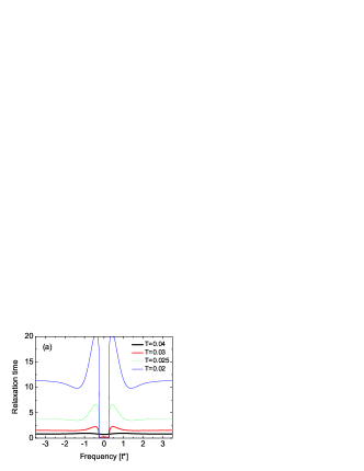
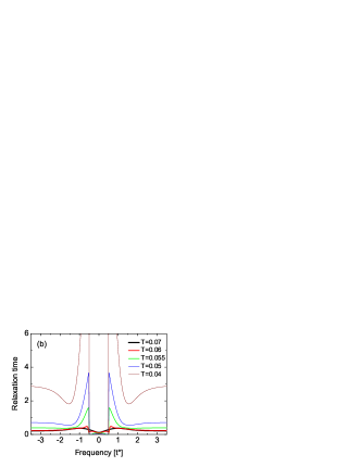
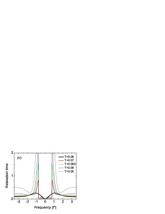
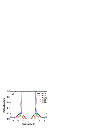
Figure 7: (Color online) Exact many-body relaxation time at various $T$ values for the CDW-ordered phase on a hypercubic lattice with (a) $U=0.5$, (b) $U=1$, (c) $U=1.5$, and (d) $U=2.5$. At high $T$ in the Mott-insulator, the relaxation time goes to zero as $\omega^{4}$ [this is hard to see in panel (d) because the quartic region occurs only for small frequencies and cannot be easily seen on this linear scale plot].

The final formalism we need to develop is for the dc transport properties. Starting from the expression for the optical conductivity in Eq. (40) we can calculate the dc conductivity by taking the zero frequency limit:

$$\sigma_{dc}=\lim\limits_{\omega\to 0}\sigma(\omega).$$ (41)

The algebra is completely straightforward, but requires a careful use of l’Hôpital’s rule for determining some of the limits. After some lengthy algebra, we find that the final expression of the dc conductivity becomes

$$\sigma_{dc}=2\int\limits_{-\infty}^{+\infty}d\omega\left[-\dfrac{df(\omega)}{d\omega}\right]\tau(\omega)$$ (42)

with the exact many-body relaxation time $\tau(\omega)$ equal to

$$\tau(\omega) =\dfrac{1}{4\pi^{2}}\Biggl{\{}\dfrac{1}{2}\biggl{[}\dfrac{\operatorname{Re}\left\{[\omega+\mu_{d}^{A}-\Sigma^{A}(\omega)][\omega+\mu_{d}^{B}-\Sigma^{B*}(\omega)]\right\}}{|\bar{Z}(\omega)|^{2}}\left\{\dfrac{\operatorname{Re}F_{z}(\omega)}{\operatorname{Re}\bar{Z}(\omega)}-\dfrac{\operatorname{Im}F_{z}(\omega)}{\operatorname{Im}\bar{Z}(\omega)}\right\}$$

$$-\left\{\dfrac{\operatorname{Re}F_{z}(\omega)}{\operatorname{Re}\bar{Z}(\omega)}+\dfrac{\operatorname{Im}F_{z}(\omega)}{\operatorname{Im}\bar{Z}(\omega)}\right\}\biggr{]}-2\operatorname{Re}[\bar{Z}(\omega)F_{z}(\omega)-1]\Biggr{\}}.$$ (43)

For large frequencies the relaxation time approaches the asymptotic value

$$\tau_{\infty}=\dfrac{1}{4\pi^{2}}\frac{2}{U^{2}[n_{f}^{A}(1-n_{f}^{A})+n_{f}^{B}(1-n_{f}^{B})]};$$ (44)

this is a well-known anomaly on the infinite-dimensional hypercubic latticedemchenko due to the fact that the DOS never vanishes and at large frequencies the imaginary part of the self-energy is exponentially small, implying very long lifetimes for the excitations. Note that the high-frequency limit of $\tau(\omega)$ actually diverges as $T\rightarrow 0$ at half filling. This trend can be seen to develop in Fig. 7, although we do not push the calculations too low in temperature due to accuracy issues with determining the subgap states.

Starting from Eq. (42) we can also calculate the thermal transport. Since the system is at half-filling, the thermopower vanishes due to particle-hole symmetry: the relaxation time in Eq. (II) is symmetric with respect to sublattice indices and is an even function of frequency at half-filling (Fig. 7). The electronic contribution to the thermal conductivity $\kappa_{e}$ is nonzero, and can be found in the standard fashion. It is expressed in terms of three different transport coefficients $L_{11}$, $L_{12}=L_{21}$ and $L_{22}$ as follows: luttinger

$$\kappa_{e}=\dfrac{1}{T}\left[L_{22}-\dfrac{L_{12}L_{21}}{L_{11}}\right].$$ (45)

In this notation, the dc conductivity satisfies

$$\sigma_{dc}=L_{11}.$$ (46)

The other transport coefficients can be calculated from the Jonson-Mahan theoremJMT1 ; JMT2 which says that there is a simple relation between these different transport coefficients, namely that they reproduce the so-called Mott-Thellung noninteracting formCT ,

$$L_{ij}=\int\limits_{-\infty}^{+\infty}d\omega\left[-\dfrac{df(\omega)}{d\omega}\right]\tau(\omega)\omega^{i+j-2},$$ (47)

where $\tau(\omega)$ is the exact many-body relaxation time defined in Eq. (II) and plotted in Fig. 7.

III Numerical Results

We begin our discussion on transport properties in the ordered CDW phase by examining the optical conductivity. In Fig. 8 we plot the temperature dependence of the optical conductivity for a dirty metal with $U=0.5$. At high temperatures we see the expected behavior for a dirty metal—namely, there is a peak at low energy and a spread on the order of the metallic bandwidth. The system does not have a low energy fermi liquid peak, because it is not a fermi liquid. Below the critical temperature for CDW order, the shape of the optical conductivity changes significantly. Note how the spectral weight is shifted upward in frequency because the system is becoming an insulator at low $T$. In particular, a sharp peak develops at $\omega=U$ which corresponds to the interband transitions from the lower band at $\tilde{\omega}<-U/2$ to the upper band at $\tilde{\omega}>U/2$. We also see two additional peaks at lower frequencies. The higher of those peaks corresponds to transitions from the lower band to the subgap states above the chemical potential and from the subgap states below the chemical potential to the upper band and the lower one corresponds to the transitions between the subgap states below and above the chemical potential. Both of these lower energy peaks must vanish as $T\rightarrow 0$ because the subgap states disappear continuously at $T=0$. Note that the frequency $\omega=U$ divides the spectra into two parts: to the right of this point the intensity of spectra increases as $T$ decreases and to the left of this point the intensity decreases as $T$ decreases which is similar to the isosbestic behavior of Mott insulators in the homogeneous phase, although we don’t see the same kind of isosbestic behavior in the ordered-phase optical conductivity here.

Results for $U=1$ have a similar structure to those for $U=0.5$, so we do not show them here.

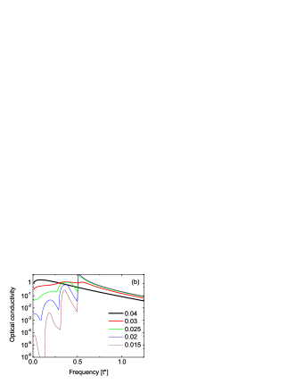
Figure 8: (Color online) Optical conductivity for $U=0.5$ and various temperatures. Panel (a) is a linear scale and panel (b) is a logarithmic scale.

We next plot the optical conductivity for a near critical Mott insulator ($U=1.5$) in Fig. 9. Here we see similar structure, with the peaks shifting to higher energy as $T$ decreases, but the overall effect is not as large as in the metal, because this system would be an insulator even if there was no CDW order. Nevertheless, we still see the large peak develop with an edge at $\omega=U$, and we see two low-energy peaks that have strong temperature dependence due to the types of transitions involving subgap states described above.

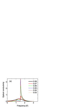
Figure 9: (Color online) Optical conductivity for $U=1.5$ and various temperatures. Panel (a) is a linear scale and panel (b) is a logarithmic scale.

Finally, we plot results for a moderate gap Mott insulator ($U=2.5$) in Fig. 10. The behavior here is essentially identical to what we saw at smaller values of $U$, except the effects are smaller, because the subgap states are very small for frequencies below where the Mott gap region extends, so the overall effects are somewhat reduced. But all of the qualitative behavior remains.

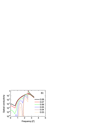
Figure 10: (Color online) Optical conductivity for $U=2.5$ and various temperatures. Panel (a) is a linear scale and panel (b) is a logarithmic scale.

In order to complete our discussion of the dynamical response, we now describe the optical sum rule. In general, the sum rule for the optical conductivity is

$$\int_{0}^{\infty}d\omega\sigma(\omega)=-\pi K,$$ (48)

where $K$ is the average kinetic energy (which is always nonpositive). In the CDW-ordered phase the average kinetic energy is equal to

$$K =T\sum_{m}\frac{1}{2N}\sum_{\bm{k}}\epsilon_{\bm{k}}\left[G_{m{\bm{k}}}^{AB}+G_{m{\bm{k}}}^{BA}\right]$$

$$=T\sum_{m}[\bar{Z}_{m}F_{zm}-1]=T\sum_{m}\lambda_{m}^{A}G_{m}^{A}=T\sum_{m}\lambda_{m}^{B}G_{m}^{B}$$

$$=-\frac{1}{\pi}\int d\omega f(\omega)\operatorname{Im}\lambda^{a}(\omega)G^{a}(\omega),\quad a=A,B,$$ (49)

and at $T=0$, when $\Sigma^{A}=U$ and $\Sigma^{B}=0$, we immediately find

$$K=-\frac{1}{2}\int d\epsilon\rho(\epsilon)\frac{\epsilon^{2}}{\sqrt{\frac{U^{2}}{4}+\epsilon^{2}}}.$$ (50)

In Fig. 11, we plot the average kinetic energy both for the CDW and homogeneous solutions for different values of $U$ at $T=0$. For small values of $U$ ($U<0.648$), we observe the anticipated behavior that the average kinetic energy increases faster in the ordered phase than in the homogeneous phase. This is anticipated because the homogeneous phase has, on average, some neighboring sites with no localized electrons, implying hopping is easier than in the ordered phase, where every hop involves a change in energy by $U$ at $T=0$ because the order parameter is uniform on each sublattice. Since it is more difficult to hop in the ordered phase, the kinetic energy increases relative to the homogeneous phase. For large values of $U$ we find anomalous behavior, where the average kinetic energy is more negative in the ordered phase. There is no simple picture to explain how this occurs. In the homogeneous phase, as $U$ increases, it becomes more difficult to hop because the doubly occupied states are being projected out of the system. This implies the average kinetic energy increases in the homogeneous phase, but it does so faster than in the ordered phase. The subtle details of how the average kinetic energy evolves with temperature are shown in Fig. 12. The anomalous behavior for the temperature dependence of the average kinetic energy occurs for a finite range of $T$ when $U>0.52$. This is the “critical” $U$ value where the DOS in the normal state changes its curvature from being negative at the chemical potential, as expected for a conventional metal, to positive in what is sometimes called an anomalous metal. In the region $0.52<U<0.648$, the normal state DOS starts to develop a dip at the chemical potential, and for a finite temperature range, the anomalous behavior in the average kinetic energy occurs only for low temperatures. As $U$ is increased further, we see the anomalous behavior occur for all $T$. These results show that the spectral weight in the CDW phase shows a modest decrease for small $U$ and a dramatic increase for large $U$ at $T=0$! This is somewhat unexpected, since the behavior is different than what is seen in say a BCS superconductor, where the gap formation reduces spectral weight at high frequencies, but the lost weight is restored in a zero frequency Drude peak. For the CDW ordered phase, no zero frequency delta function appears. The spectral weight loss is small for small $U$, but the gain can become significant for large $U$.

Figure 11: The average kinetic energy $K$ for different values of $U$ at $T=0$. The solid line corresponds to the CDW phase and the dotted line corresponds to the homogeneous solution.

Figure 12: Temperature dependence of the average kinetic energy for different values of $U$: (a) $U=0.5$; (b) $U=0.52$; (c) $U=0.645$; (d) $U=1$. The solid line corresponds to the CDW phase and the dotted line corresponds to the homogeneous solution.

Next we examine the dc transport. The temperature dependence of the dc and thermal conductivity are plotted in Figs. 13 and 14, respectively, where we plot both the CDW solution and the homogeneous solution extrapolated into the CDW region. At low temperatures, due to the factor $-df(\omega)/d\omega$, the main contributions to the dc transport come from the narrow region of width $4T$ around the chemical potential (the so-called fermi window). For the Falicov-Kimball model at half filling in the homogeneous phase ($T>T_{c}$) the DOS, Green’s functions and self-energies do not depend on temperature and, as a result, the temperature dependence of the dc transport is determined solely by the shape of the relaxation time in Eq. (II) close to the chemical potential. For small $U$ values the relaxation time $\tau(\omega)$ is flat [Fig. 7 (a)] and, as a result, the dc conductivity for the homogeneous phase is essentially a constant for low $T$. At $U=\sqrt{2}$ the Mott insulator forms. For larger $U$ values, one might expect to see exponentially activated transport, but that does not occur on the hypercubic lattice, because the system only possesses a pseudogap. Even though the DOS exponentially decreases in the gap region, the lifetime of the excitations is exponentially long, and $\tau(\omega)$ behaves like $\omega^{4}$ for low energiesdemchenko . This produces a quartic dependence of the dc conductivity on $T$, and a higher power law for the thermal conductivity.

In the CDW phase ($T<T_{c}$), the CDW gap is filled by subgap states at finite $T$, which lead to a less severe modification of the exponentially activated transport at low $T$. But it is only the subgap states within the fermi window that affect the transport, so the modification is not quite as severe as one might have naively guessed. Note the small wiggles in the solid lines at low $T$. These occur due to the evolution of the subgap states. The $T$ dependence of the dc transport always shows a marked kink at $T_{c}$ with the conductivities sharply suppressed as the CDW gap forms. In the Mott insulator, the transport changes from power law in $T$ to exponential activation (suitably modified by the subgap states). The thermal conductivity displays similar features, as shown in Fig. 14.

Figure 13: dc conductivity for (a) $U=0.5$ ($T_{c}\approx 0.034$), (b) $U=1$ ($T_{c}\approx 0.0615$), (c) $U=1.5$ ($T_{c}\approx 0.075$) and (d) $U=2.5$ ($T_{c}\approx 0.072$) as a function of temperature. The solid line denotes the CDW ordered phase and the dashed line denotes the homogeneous one. Results are presented on a linear scale (left) and logarithm of dc conductivity vs inverse temperature (right).

Figure 14: Electronic contribution to the thermal conductivity for (a) $U=0.5$ ($T_{c}\approx 0.034$), and (b) $U=2.5$ ($T_{c}\approx 0.072$) as a function of temperature. The solid line denotes the CDW ordered phase and the dashed line denotes the homogeneous one. Results are presented on a linear scale (left) and logarithm of thermal conductivity vs inverse temperature (right).

IV Conclusions

In this work we have developed the formalism to calculate transport properties of CDW-ordered phases within DMFT. Since the dc charge and heat transport and the optical conductivity continue to have no vertex corrections, even in the ordered phase, the calculations reduce to a careful evaluation of the bare Feynman diagrams with a sublattice index introduced by the order.

As the system orders into a CDW state, the DOS develops a gap with a sharp singularity in the DOS at the band edge when $T=0$. The gap at $T=0$ is always equal to $U$. As the temperature increases, but still below $T_{c}$, we see a significant development and evolution of subgap states within the gap region. This gap region where subgap states develop, appears to lie within the extent of the normal-state DOS—in other words, in the Mott insulator, we do not see subgap states develop within the region that corresponds to the Mott gap in the normal state. We verify the accuracy of the DOS calculations by calculating the zeroth, first, and second moment of the local DOS on each sublattice and we find they agree with exact results to essentially machine accuracy.

The optical conductivity has a significant rearrangement of states within the ordered phase, which can be understood by examining the different kinds of processes that take place within an optical transition—namely that we move from an occupied to an unoccupied state. Because there are many different bands that are present at finite $T$, this leads to significant structure in the optical conductivity. In particular, the singularity in the DOS leads to a large asymmetric peak centered around $U$ in the response function. The total spectral weight is governed by the average kinetic energy due to the optical sum rule. While a naive expectation would say the average kinetic energy increases when the ordering is turned on (i. e., it becomes less negative with a smaller magnitude) because the ordering blocks hopping between the sublattices, we find that is true only for small $U$. For small $U$ the kinetic energy shows a modest increase, so some spectral weight is lost due to the ordering. For larger $U$ the kinetic energy shows a significant reduction (i. e., the magnitude increases as the average kinetic energy becomes more negative) so the spectral weight increases when the ordered phase is entered, and that increase can become quite substantial as $U$ becomes large.

Finally, we also examined the dc transport. Since we are at half filling, one can show the thermopower vanishes due to particle-hole symmetry even in the presence of CDW order. Hence we can only examine the charge and heat conductivities. We find that the CDW order suppresses both of these, but because of the subgap states and their complicated evolution with temperature, the dc response does not obey any simple functional form at low $T$. Instead, we often see significant wiggles in the conductivities. In the Mott-insulating phase, the conductivity should go from a power-law-like behavior to exponential activation. We see such a trend start to develop, but we cannot accurately quantify this because we cannot go down far enough in temperature in the CDW phase before we run into issues with accuracy of the calculations.

This work shows that there is rich and interesting behavior that occurs in the transport as CDW order sets in. In future work, we will examine Raman scattering, where vertex correction effects are present and inelastic X-ray scattering, where interesting phenomena is likely to occur when the photon transfers momentum equal to the ordering wavevector.

- (1) U. Brandt and C. Mielsch, Z. Phys. B: Condens. Matter 75, 365 (1989).
- (2) W. Metzner and D. Vollhardt, Phys. Rev. Lett. 62, 324 (1989).
- (3) A. Georges, G. Kotliar, W. Krauth, and M. J. Rozenberg, Rev. Mod. Phys. 68, 13 (1996).
- (4) U. Brandt and C. Mielsch, Z. Phys. B: Condens. Matter 79, 295 (1990).
- (5) P. G. J. van Dongen, Phys. Rev. B 45, 2267 (1992).
- (6) L. Chen, B. A. Jones, and J. K. Freericks, Phys. Rev. B 68, 153102 (2003).
- (7) C. Gruber, N. Macris, P. Royer, and J. K. Freericks, Phys. Rev. B 63, 165111 (2001).
- (8) S. Tajima, S. Uchida, A. Masaki, H. Takagi, K. Kitazawa, S. Tanaka, and A. Katsui, Phys. Rev. B 32, 6302 (1985); S. Tajima, S. Uchida, A. Masaki, H. Takagi, K. Kitazawa, S. Tanaka, and S. Sugai, Phys. Rev. B 35, 696 (1987); S. Sato, S. Tajima, H. Takagi, and S. Uchida, Nature 338, 241 (1989); S.H. Blanton, R.T. Collins, K.H. Kelleher, L.D. Rotter, Z. Schlesinger, D.G. Hinks, and Y. Zheng, Phys. Rev. B 47, 996 (1993); M.A. Karlow, S.L. Cooper, A.L. Kotz, M.V. Klein, P.D. Han, and D.A. Payne, Phys. Rev. B 48, 6499 (1993); R.P.S.M. Lobo and F. Gervais, Phys. Rev. B 52, 13294 (1995); Hyun-Tak Kim, Phys. Rev. B 54, 90 (1996); S.M. Hasanuzzaman, Kaoru Iwano, and Keiichiro Nasu, J. Phys. Soc. Japan 68, 1376 (1999).
- (9) L. M. Falicov and J. C. Kimball, Phys. Rev. Lett. 22, 997 (1969).
- (10) J. K. Freericks and V. Zlatić, Rev. Mod. Phys. 75, 1333 (2003).
- (11) V. Zlatić, J. K. Freericks, R. Lemański, and G. Czycholl, Phil. Mag. B 81, 1443 (2001).
- (12) W. Metzner, Phys. Rev. B 43, 8549 (1991).
- (13) S. R. White, Phys. Rev. B 44, 4670 (1990).
- (14) V. M. Turkowski and J. K. Freericks, Phys. Rev. B 73, 075108 (2006); Erratum, Phys. Rev. B 73, 209902(E) (2006).
- (15) R. Kubo, J. Phys. Soc. Japan 12, 570 (1957).
- (16) D. A. Greenwood, Proc. Phys. Soc. London 71, 585 (1959).
- (17) A. Khurana, Phys. Rev. Lett. 64, 1990 (1990).
- (18) J. K. Freericks, D. Demchenko, A. Joura, and V. Zlatić, Phys. Rev. B 68, 195120 (2003).
- (19) J. M. Luttinger, Phys. Rev. 135, A1505 (1964).
- (20) M. Jonson and G. D. Mahan, Phys. Rev. B 21, 4223 (1980).
- (21) M. Jonson and G. D. Mahan, Phys. Rev. B 42, 9350 (1990).
- (22) G. V. Chester and A. Thellung, Proc. Phys. Soc. London 77, 1005 (1961).